at SciVerse ScienceDirect

Atmospheric Environment 77 (2013) 748e756

Contents lists available

Atmospheric Environment

journal homepage: www.elsevier .com/locate/atmosenv

RLINE: A line source dispersion model for near-surface releases

Michelle G. Snyder a,*, Akula Venkatramb, David K. Heist a, Steven G. Perry a,William B. Petersen c, Vlad Isakov a

aU.S. Environmental Protection Agency, Office of Research and Development, National Exposure Research Laboratory, Atmospheric Modeling and AnalysisDivision, Research Triangle Park, NC 27711, USAbUniversity of California, Riverside, CA 92521, USAcWilliam B. Petersen Consulting, Research Triangle Park, NC, USA

h i g h l i g h t s

� We have developed a new Research LINE source dispersion model (RLINE).� RLINE utilizes hourly meteorology and simplified source & receptor specifications.� A new formulation for near-surface dispersion is implemented in numerical routine.� Model development & evaluation shown for Idaho Falls Experiment (Finn et al., 2010).� Evaluation includes Caltrans (Benson, 1989) and Raleigh NO (Baldauf et al., 2008).

a r t i c l e i n f o

Article history:Received 2 January 2013Received in revised form23 May 2013Accepted 28 May 2013

Keywords:Near-surface dispersionNear-road concentrationsSurface releasesSimilarity theoryMeteorological measurementsUrban dispersionIdaho falls experimentRLINE

* Corresponding author.E-mail address: Snyder.Michelle@epa.gov (M.G. Sn

1352-2310/$ e see front matter Published by Elsevierhttp://dx.doi.org/10.1016/j.atmosenv.2013.05.074

a b s t r a c t

This paper describes the formulation and evaluation of RLINE, a Research LINE source model for near-surface releases. The model is designed to simulate mobile source pollutant dispersion to support theassessment of human exposures in near-roadway environments where a significant portion of thepopulation spends time. The model uses an efficient numerical integration scheme to integrate thecontributions of point sources used to represent a line-source. Emphasis has been placed on estimates ofconcentrations very near to the source line. The near-surface dispersion algorithms are based on newformulations of horizontal and vertical dispersion within the atmospheric surface layer, details of whichare described in a companion paper (Venkatram et al., 2013). This paper describes the general formu-lations of the RLINE model, the meteorological inputs for the model, the numerical integration tech-niques, the handling of receptors close to the line source, and the performance of the model againstdevelopmental data bases and near-road concentrations from independent field studies conducted alongactual highway segments.

Published by Elsevier Ltd.

1. Introduction

Growing concern about human exposure and related adversehealth effects near roadways motivated an effort by the U. S.Environmental Protection Agency to reexamine the dispersion ofmobile source related pollutants. Studies have shown that livingnear roadways is implicated in adverse health effects includingrespiratory problems (e.g. McCreanor et al., 2007), birth anddevelopmental defects (Wilhelm and Ritz, 2003), premature mor-tality (e.g. Krewski et al., 2009), cardiovascular effects (Peters et al.,2004; Riediker et al., 2004) and cancer (Harrison et al., 1999;

yder).

Ltd.

Pearson et al., 2000). These studies of traffic-related health effectshave included both short-term (e.g., hourly) and long-term (e.g.,annual) exposures (Krewski et al., 2009; McCreanor et al., 2007).

Estimating exposure to roadway emissions requires dispersionmodeling to capture the temporal and spatial variability of mobilesource pollutants in the near-road environment. The model needsto account for the variability in mobile emissions across a myriad ofurban and suburban landscapes, while considering factors(depending on pollutant and application scenario) such as vehicleinduced turbulence, roadway configurations (e.g. depressed road-ways and noise barriers), local meteorology, surrounding terrainand buildings, pollutant chemistry, deposition, and others.

There are several models in the literature that have beendeveloped to simulate dispersion from roadways. Examples include

M.G. Snyder et al. / Atmospheric Environment 77 (2013) 748e756 749

HIWAY-2 (Petersen, 1980), UCD (Held et al., 2003), CAR-FMI(Harkonen et al., 1995), GM (Chock, 1978), OSPM (Hertel andBerkowicz, 1989), ADMS-ROADS (McHugh et al., 1997), CFD-VIT-RIT (Wang and Zhang, 2009) and the CALINE series of models(Benson, 1989, 1992). Because urban areas typically contain a largenumber of road segments, computational efficiency is an importantfactor in formulating a line source dispersion model. As a result,most models for dispersion of roadway emissions are analyticalapproximations to the integral associated with modeling a linesource as a set of point sources. However, these approximations canlead to large errors when thewinds are light and variable, when thewind direction is close to parallel to the road and when the sourceand receptor are at different heights (Briant et al., 2011). So thecurrent version of RLINE is based on Romberg numerical integra-tion of the contributions of point sources along a line (roadsegment). This approach allows us to incorporate the governingprocesses without introducing errors associated with approxi-mating the underlying model framework.

The point contributions along the line source are computedwiththe Gaussian, steady-state plume formulation. This is consistentwithmodels currently recommended by the U. S. EPA for regulatoryapplications e.g. CALINE3 (Benson, 1992) and AERMOD (Cimorelliet al., 2005).

RLINE is designed to simulate primary, chemically inert pol-lutants with emphasis on near surface releases and near sourcedispersion. The model has several features that distinguishes itfrom other models. It includes new formulations for the verticaland horizontal plume spread of near surface releases based onhistorical field data (Prairie Grass, Barad, 1958) as well as a recenttracer field study (Finn et al., 2010) and recent wind tunnel studies(Heist et al., 2009). Details of the formulations are found in thecompanion paper by Venkatram et al. (2013). Additionally, themodel contains a wind meander algorithm that accounts fordispersion in all directions during light and variable winds. Tofacilitate application of the model, its meteorological inputs areconsistent with those used by the AERMOD model (Cimorelliet al., 2005). In addition to evaluation against the Finn et al.,2010 tracer data, the model has been compared with measure-ments from two independent field studies performed along actualhighway segments covering a wide range of meteorological con-ditions (Baldauf et al., 2008; Benson, 1989). The current version ofRLINE applies for flat roadways. However, the model framework isdesigned to facilitate the inclusion of algorithms for depressedroadways and roadways with noise barrier. These complexroadway algorithms will be included in a near future version ofthe model.

This paper describes the general formulations of the RLINEmodel including new horizontal and dispersion formulations,the handling of receptors very close to the source, and themeteorological inputs for the model. Then, we evaluate per-formance of the model against both a developmental data baseand near-road concentrations from two independent fieldstudies.

2. The line source model

The concentration from a finite line source in RLINE is found byapproximating the line as a series of point sources. The number ofpoints needed for convergence to the proper solution is determinedby the model and, in particular, is a function of distance from thesource line to the receptor. Each point source is simulated using aGaussian plume formulation. Here we explain the implementationof the point source plume model and the integration scheme usedto approximate a line source. We begin with a description of themeteorological inputs needed for the model.

2.1. Meteorological inputs

The meteorology that drives RLINE is obtained from the surfacefile output from AERMOD’s met processor, AERMET (Cimorelliet al., 2005). AERMET processes surface characteristics (surfaceroughness, moisture and albedo), cloud cover, upper air temper-ature soundings, near surface wind speed, wind direction andtemperature to compute the surface variables needed by AERMOD.The specific variables that are needed by RLINE include the surfacefriction velocity (u*), the convective velocity scale (w*), MonineObukhov length (L), the surface roughness height (zo), and thewind speed and direction at a reference height within the surfacelayer.

Additionally, for light wind, stable conditions, when u* isgenerally small, an adjustment is made to the friction velocitybased on the work of (Qian and Venkatram, 2011). From an ex-amination of stable periods within meteorological field measure-ments collected in Cardington, Bedfordshire as wind speedsbecame small Qian and Venkatram found that u* was much largerthan values predicted by those from AERMET. From the formula-tions in AERMET and assuming a constant value of the temperaturescale, T* ¼ w0T 0=u* ¼ 0.08, where w’T ’ is the mean vertical tem-perature flux, u* takes the form

u* ¼ C1=2DN Ur

2

h1þ

�1� r2

�1=2i(1)

where

CDN ¼ k2�ln�zr�dhz0

��2 ; (2)

r ¼ UcritUr

; (3)

Ucrit ¼ 2u0C1=4DN

; (4)

and

u0 ¼�bgðzr � dh � z0ÞT*

T0

�1=2

(5)

where dh is the canopy displacement height, k the von karmanconstant, Ur is the wind speed measured at the reference height, zrand To is the temperature at reference height.

Qian and Venkatram recommend the following modification toEqn. (1) for cases of light winds (low u*) and stable atmosphericconditions (L > 0)

u* ¼ C1 =

2

DNUr

2

�1þ exp

��r2=2�

1� expð�2=rÞ

(6)

Once u* has been adjusted for light wind, then L and all otherparameters affected by this adjustment are recalculated using theAERMET methodology for internal consistency.

RLINE has a lower limit for the effective wind speed used in thedispersion calculations that is a function of the lateral turbulence.The horizontal wind energy is composed of a mean component u2

and two random wind energy components, su2 and sv2. Assuming

these random components to be approximately equal, when themean wind goes to zero, the horizontal wind energy will maintainat 2sv2. Therefore, the minimum effective wind speed is set at

M.G. Snyder et al. / Atmospheric Environment 77 (2013) 748e756750

ffiffiffi2

p$sv: From (Cimorelli et al., 2005), the lateral turbulent wind

component is computed as

sv ¼ffiffiffiffiffiffiffiffiffiffiffiffiffiffiffiffiffiffiffiffiffiffiffiffiffiffiffiffiffiffiffiffiffiffiffiffiffiffiffiffiffiffiffið0:6w*Þ2 þ ð1:9u*Þ2

q(7)

where w* is the convective velocity scale.Therefore, the effective wind speed is:

Ue ¼ffiffiffiffiffiffiffiffiffiffiffiffiffiffiffiffiffiffiffiffiffiffiffiffiffiffi2s2v þ UðzÞ2

q: (8)

Here the wind speed, U, is evaluated at the mean plume height,z. The mean plume height depends on the vertical spread of theGaussian plume, which will be described in Section 2.3.1.

2.2. Numerical line source approximation

The mathematical formulation to compute the impact of a linesource is simplified by using a coordinate system where the Y-axislies along the line source as shown in Fig. 1. The wind direction isoriented at an angle, q, relative to the X-axis, and the receptor co-ordinates are given by (Xr, Yr, Zr).

If L is the length of the source, Y2 ¼ Y1 þ L. To calculate theconcentration at a receptor (Xr, Yr, Zr) caused by emissions from theline source characterized by an emission rate of q (mass/(time*-length)), we represent the line source by a set of point sources ofstrength q$dY along the line Y1Y2.

The contribution of the plume originating at Ys to the receptorconcentration is most conveniently expressed in a co-ordinatesystem, xey, with its origin at (0,Ys), and the x-axis along the di-rection of the meanwind; the x-axis is rotated by an angle q relativeto the fixed X-axis.

The horizontal co-ordinates of the receptor in the along-windcoordinate system, (xr, yr, zr), can be expressed as

xr ¼ Xrcos qþ ðYr � YsÞsin qyr ¼ ðYr � YsÞcos q� Xrsin q

(9)

The vertical coordinate remains unchanged so that zr ¼ Zr.Then, the concentration at (xr,yr) due to the line becomes

Cðxr; yrÞ ¼ZY1þL

Y1

dCpt ; (10)

where dCpt is the contribution from an elemental point source.

Fig. 1. Co-ordinate systems used to calculate contribution of point source at Ys toconcentration at (Xr,Yr, Zr). The system xey has the x-axis along the mean wind di-rection, which is at an angle q to the fixed X axis. The dotted line is a representation ofthe plume.

The point-source Gaussian plume formulation is the sum ofplume components (horizontal and vertical with subscript pl) andmeandering contributions (with subscript m). The plume compo-nent centerline follows the wind direction, as in Fig. 1, and themeandering component, accounting for the random component ofthe wind, spreads the plume material radially outward from thesource equally in all directions. The two components are addedusing a weighting factor, f, based on the magnitudes of the lateralturbulence and the mean wind.

dCpt ¼ ð1� f Þ$dCpl þ f $dCm (11)

where

f ¼ 2$s2vU2e

(12)

Because Ue has a minimum value offfiffiffiffiffiffiffiffi2s2v

q, f is limited to be-

tween 0 and 1.The plume concentration is broken into the vertical and hori-

zontal components,

dCpl ¼qdYsUe

hVERT$HORZpl

i; (13)

where q is the emission rate.The meander component is given by

dCm ¼ qdYsUe

½VERT$HORZm� (14)

The vertical component of the plume and meander concentra-tions is found by

VERT¼ 1ffiffiffiffiffiffiffi2p

psz

$

"exp

�12

�zs�zrsz

�2!þexp

�12

�zsþzrsz

�2!#

;

(15)

where the vertical spread, sz, will be described in Section 2.3.1. Thehorizontal plume component is found by

HORZpl ¼1ffiffiffiffiffiffiffi2p

psy

exp

� 12

�yr � yssy

�2!; (16)

where the horizontal spread, sy, will be described in Section 2.3.2.Under lowwind speeds, horizontal meander tends to spread the

plume over large azimuth angles, which might even lead to con-centrations upwind relative to the vector averaged wind direction.Adopting the approach in Cimorelli et al. (2005) we assume that asthe wind speed approaches zero, the horizontal plume spreadsequally in all directions. Thus the horizontal meander componentin Equation (15) has the form

HORZm ¼ 12$p$R

R ¼ffiffiffiffiffiffiffiffiffiffiffiffiffiffiffiffiffiffiffiffiffiffiffiffiffiffiffiffiffiffiffiffiffiffiffiffiffiffiffiffiffiffiffiffiffiffiffiðxr � xsÞ2 þ ðyr � ysÞ2

q (17)

In the Gaussian point source formulation the concentration goesto infinity as the distance between the source and the receptor goesto zero (since sy and sz also go to zero). Therefore, for receptors verynear the source, the model sets the minimum distance (along thewind direction) between the receptor and the line source to one-meter.

M.G. Snyder et al. / Atmospheric Environment 77 (2013) 748e756 751

2.3. New dispersion formulations

Near surface dispersion has been studied extensively since the1950s. The Prairie Grass experiment (PG) (Barad, 1958), provided acomprehensive data base that has been used by several authors toformulate dispersion models for near surface releases (e.g. Briggs,1982; van Ulden, 1978; Venkatram, 1992). A new tracer study(Finn et al., 2010) examining dispersion from a near surface linerelease provided an opportunity to re-examine the formulations ofsz and sy in Equations (16) and (17). The companion paper(Venkatram et al., 2013) provides a detailed reformulation of thedispersion parameters. The resultant formula incorporated intoRLINE are included here.

2.3.1. Vertical spreadThe starting point of the vertical spread reformulation is the

solution of the eddy diffusivity based mass conservation equationproposed by van Ulden (1978). Venkatram et al. (2013) proposes aninterpolation between the limits of very stable and neutral condi-tions to establish a relationship between the mean plume height, z,and the vertical plume spread, sz. In stable conditions, the verticalspread is given by

sz ¼ au*Ue

x1�

1þ bsu*

Ue

�xL

�2=3� ; (18)

where the constants, a and bs, are obtained empirically. Similarly,for unstable conditions the vertical spread is found to be

sz ¼ au*Ue

x�1þ bu

�u*Ue

xL

��: (19)

where bu is an empirical constant for unstable conditions. Note thatthese expressions for sz are implicit because the wind speed, Ue, onthe right hand side of the equation is a function of z, which in turn isa function of sz. Note also that the expressions for stable (Equation(18)) and unstable (Equation (19)) conditions reduce to the sameneutral limit for large L.

Based on the evaluation of Equations (18) and (19) against thePrairie Grass and the Idaho Falls tracer experiments, Venkatramet al. (2013) find the following best fit to the coefficients:a ¼ 0.57, bs ¼ 3, and bu ¼ 1.5.

The mean plume height, where Ue is evaluated (see Equation(8)), is found to be a function of the vertical spread (Venkatramet al., 2013), and has the form:

z ¼ sz

ffiffiffiffi2p

rexp

�� 12

�zssz

�2þ zserf

�zsffiffiffi2

psz

�: (20)

2.3.2. Horizontal spreadEstimates of horizontal dispersion in the surface layer have

largely been based on Taylor’s theory (1921) for dispersion in ho-mogeneous turbulence which is based on the Lagrangian time scaleand sv. Unfortunately, the plume travel time cannot be definedunambiguously because the wind speed varies with height. Weavoid this problem by using an approach suggested by Eckman(1994), who showed that the variation of sy with distance couldbe explained by the variation of the effective transport wind speed,even when the standard deviation of the horizontal velocity fluc-tuations is constant with height. Venkatram et al. (2013) use Eck-man’s equation to derive expressions such that

sy ¼ csvu

sz

�1þ ds

szjLj�; for stable conditions (21)

*

and

sy ¼ csvu*

sz

�1þ du

szjLj��1=2

; for unstable conditions (22)

where c, ds, and du are empirical constants. Based on the evaluationof Equations (21) and (22) against the Prairie Grass data, the best fitvalues for the constants are: c ¼ 1.6, ds ¼ 2.5, and du ¼ 1.0. As withthe vertical spread, a detailed discussion of the horizontal spreadformulation is found in Venkatram et al. (2013).

2.4. Numerical computation of concentration

The right hand side of Equation (10) must be integratednumerically because both sy and sz depend on xr, which in turn is afunction of the integrating variable Ys (See Equation (9)). This isdone in RLINE with an efficient Romberg integration scheme (Presset al., 1992). Convergence of the scheme is assumed when thedifference between estimated concentration is below a user spec-ified error limit (recommended 1 � 10�3). When multiple sourcesare modeled the cumulative concentration is reported, but eachsource’s contribution is calculated with an accuracy of the userdefined limit.

In some cases, such as modeling pedestrian or bike-lane expo-sures it may be necessary to estimate concentrations within a fewmeters of the source. When the receptor is close to the line sourceand its concentration in the early steps of the integration scheme isdominated by a single point source or has little or no impact fromany point, convergence may occur too quickly. Therefore a mini-mum number of iterations, jmin, is calculated that prevents thispremature convergence by ensuring that the spacing between thepoints used to approximate the line source, dr, is smaller than thedistance from receptor to the line. Starting from the fact that for thejth iteration, the number of points representing the line is 2j�1 þ1,we find that:

Ldr

< 2j�1 þ 1 (23)

jmin ¼ Qlog�

2Ldrsin q

� 2�

log2S; (24)

where L is the length of the line and drsin q is the perpendiculardistance between the receptor and the line source. The case of re-ceptors very close to the line source is the most computationallytime consuming. The minimum number of iterations, jmin, can belarge when the line source is long and the distance, drsin q, be-comes small.

3. Model applications

Model performance estimates of concentration are comparedqualitatively to on-site measurements made during the two fieldstudies described below with the use of scatter plots. In addition,model performance is quantified using the performance statistics asdescribed in Venkatram (2008). The quantitative model perfor-mance measures used here are the geometric mean bias (mg), thegeometric standard deviation (sg) and the fraction of estimateswithin a factor of two of the measured value (fac2). Venkatram’sdefinitionofmg suggests that amodel is over predictivewhenmg<1.We have flipped the ratio of observed-to-predicted concentrations

M.G. Snyder et al. / Atmospheric Environment 77 (2013) 748e756752

here, so thatmg>1 is indicative of amodel over-prediction;mg<1 isindicative of amodel under-prediction. To avoid the effect of outlierson the computation of these statistics, we use the following defini-tions of the geometric mean bias and standard deviation:

mg ¼ median�CpCo

�(25)

sg ¼ exp

lnðFÞffiffiffi

2p

erf�1ðAFÞ

!; (26)

where C is the concentration, either observed (subscript ‘o’) or pre-dicted (subscript ‘p’), F is taken to be 2, AF is the fraction of the ratio,Cp/(Comg), between 1/F and F, and erf�1 is the inverse error function.Equation (26) is equivalent to fitting a lognormal distribution to thevalues of Cp/Co between 0.5 and 2, so sg equals onewhen 100% of thepredictions lie within a factor of two interval. Only when values areoutside of a factor of two interval is the value of sg greater than one.Observed andpredicted concentrations are paired in time and space.

3.1. Comparison of model to Idaho Falls tracer study

A line source experiment was conducted near Idaho Falls, Idahoin 2008 (Finn et al., 2010). The study area is located in a broad,relatively flat area on the western edge of the Snake River Plain.Five tests were conducted during the study, each spanning a 3-hperiod broken into 15-min tracer sampling intervals. One test wasconducted in unstable conditions, one in neutral conditions, andtwo in stable conditions; test 4 was not used since the wind shiftedaway from the sampler array as the test period began. A briefsummary is shown in Table 1.

The overall purpose of the study was to examine the differencein pollutant dispersion from a line-source (e.g. roadway) in thepresence and in the absence of a 90 m long and 6 m high (H) noisebarrier. Simultaneous measurements were made at the barrier andno-barrier (control) sites. Both sites had a 54 m long SF6 tracer linesource release positioned 1 m above ground level (AGL). In bothexperiments, a gridded array of bag samplers were positioneddownwind of the line source for measuring concentrations.

Mean wind and turbulence were obtained on the control sitefrom a sonic anemometer within the sampler array at a 3 m height.The roughness length scale, z0, for the sitewas estimated at 0.053mbased onmeanwind and sheer stressmeasurements from the sonicduring the near-neutral conditions of test day 1. In the developmentand evaluation of RLINE as described in this paper we have onlyused the control experiment (non-barrier) measurements.

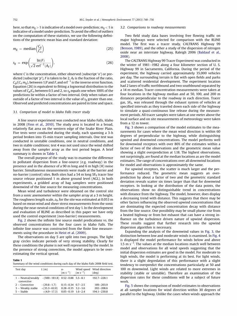
Fig. 2 shows the infinite line source model predications vs. theobserved concentrations for the four cases in Idaho Falls. Theinfinite line source was constructed from the finite line measure-ments using the procedure in Heist et al. (2009).

The observations on day 5 are split into two groups. The lightgray circles indicate periods of very strong stability. Clearly forthese conditions the plume is not well represented by the model. Inthe presence of strong convection, the model appears to be over-estimating the vertical spread.

Table 1Summary of the wind conditions during each day of the Idaho Falls 2008 field test.

Test day L (m) u*(m s�1)

Wind speed(m s�1)

Wind direction(deg)

1 e Neutral/weaklyconvective

�(500e181.8) 0.52e0.88 5.5e8.1 192.7e228.1

2 e Convective �(29.8e1.7) 0.15e0.34 0.7e2.5 189e203.93 e Weakly stable þ(35.3e62.0) 0.28e0.35 3.2e3.6 202e208.65 e Stable þ(4.9e17.3) 0.05e0.19 1.6e2.4 194.1e230.8

3.2. Comparisons to roadway measurements

Two field study data bases involving free flowing traffic onmajor highways were selected for comparison with the RLINEmodel. The first was a tracer study, CALTRANS Highway 99(Benson, 1989), and the other a study of the dispersion of nitrogenoxide near an interstate highway, Raleigh 2006 (Baldauf et al.,2008).

The CALTRANS Highway 99 Tracer Experimentwas conducted inthe winter of 1981e1982 along a four kilometer section of U. S.Highway 99 in Sacramento, California. During the period of theexperiment, the highway carried approximately 35,000 vehiclesper day. The surrounding terrain is flat with open fields and parksand scattered residential development. The experiment locationhad 2 lanes of traffic northbound and two southbound separated bya 14 m median. Tracer concentration measurements were taken atfour locations in the highway median and at 50, 100, and 200 mdistances perpendicular to the roadway in each direction. Tracergas, SF6, was released through the exhaust system of vehicles atspecified intervals as they traveled down each side of the highwayto simulate a quasi-continuous line release during the measure-ment periods. All tracer samples were taken at onemeter above thelocal surface and on site measurements of meteorology were takenfrom a 12 m tower.

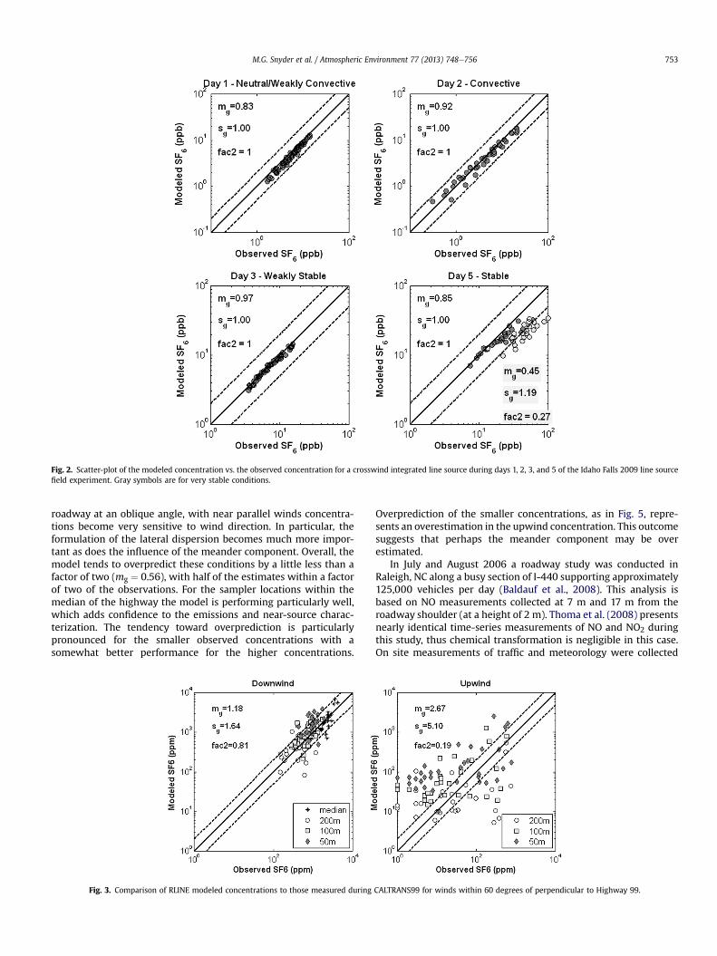
Fig. 3 shows a comparison of the model estimates to the mea-surements for cases where the mean wind direction is within 60degrees of perpendicular to the highway, while distinguishingupwind and downwind concentrations. The model performs wellfor downwind receptors with over 80% of the estimates within afactor of two of the observations and the geometric mean valueshowing a slight overprediction at 1.18. The highest observations,not surprisingly, are found at the median locations as are the modelestimates. The range of concentrations over all downwind locationsfor model and observations is approximately the same.

For upwind receptors, the scatter is much larger and the per-formance reduced. The geometric mean suggests an over-prediction by about a factor of two and the geometric standarddeviation reveals scatter six times larger than that for downwindreceptors. In looking at the distribution of the data points, theobservations show no distinguishable trend in concentrationswith distance from the highway. The model, however, does displaya decreasing trend with distance. This suggests that there may beother factors influencing the observed upwind concentrations thatare dominating the expected concentration decay with distancefrom the line source. One possibility may be small plume rise froma heated highway or from hot exhaust that can have a strong in-fluence on the turbulence driven nature of upwind dispersion.These results suggest that further research into the upwinddispersion algorithm is necessary.

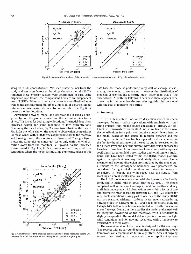
Expanding the analysis of the downwind values in Fig. 3, thedistinction between low and moderate winds is examined. In Fig. 4is displayed the model performance for winds below and above1.5 m s�1. The values at the median locations match well betweenmodel and observations for all wind speeds suggesting that theinitial dispersion estimates are good in the model. For moderate tohigh winds, the model is performing at its best. For light winds,there is a slight degredation of this performance with a slighttendency to overpredict the concentrations particularly at 50 and100 m downwind. Light winds are related to more extremes instability (stable or unstable). Therefore an examination of thedispersion rates for these conditions will be a subject of futurework.

Fig. 5 shows the comparison of model estimates to observationsat all sampler locations for wind direction within 30 degrees ofparallel to the highway. Unlike the cases when winds approach the

Fig. 2. Scatter-plot of the modeled concentration vs. the observed concentration for a crosswind integrated line source during days 1, 2, 3, and 5 of the Idaho Falls 2009 line sourcefield experiment. Gray symbols are for very stable conditions.

M.G. Snyder et al. / Atmospheric Environment 77 (2013) 748e756 753

roadway at an oblique angle, with near parallel winds concentra-tions become very sensitive to wind direction. In particular, theformulation of the lateral dispersion becomes much more impor-tant as does the influence of the meander component. Overall, themodel tends to overpredict these conditions by a little less than afactor of two (mg ¼ 0.56), with half of the estimates within a factorof two of the observations. For the sampler locations within themedian of the highway the model is performing particularly well,which adds confidence to the emissions and near-source charac-terization. The tendency toward overprediction is particularlypronounced for the smaller observed concentrations with asomewhat better performance for the higher concentrations.

Fig. 3. Comparison of RLINE modeled concentrations to those measured during

Overprediction of the smaller concentrations, as in Fig. 5, repre-sents an overestimation in the upwind concentration. This outcomesuggests that perhaps the meander component may be overestimated.

In July and August 2006 a roadway study was conducted inRaleigh, NC along a busy section of I-440 supporting approximately125,000 vehicles per day (Baldauf et al., 2008). This analysis isbased on NO measurements collected at 7 m and 17 m from theroadway shoulder (at a height of 2 m). Thoma et al. (2008) presentsnearly identical time-series measurements of NO and NO2 duringthis study, thus chemical transformation is negligible in this case.On site measurements of traffic and meteorology were collected

CALTRANS99 for winds within 60 degrees of perpendicular to Highway 99.

Fig. 4. Expansion of the analysis of the downwind concentration comparisons of Fig. 3 based on wind speed.

M.G. Snyder et al. / Atmospheric Environment 77 (2013) 748e756754

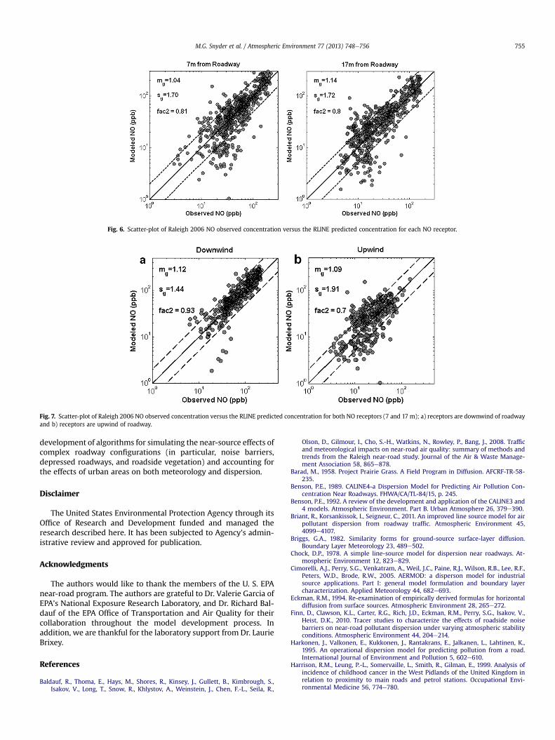
along with NO concentrations. We used traffic counts from thestudy and emission factors as found by Venkatram et al. (2007).Although these emission factors were determined, in part, usingdispersion calculations, the comparisons here are an independenttest of RLINE’s ability to capture the concentration distribution aswell as the concentration fall off as a function of distance. Modelestimates versus measured concentrations are shown in Fig. 6 forthe two monitor locations.

Agreement between model and observations is good as sug-gested by both the geometric mean and the percent within a factorof two. This is true for both sampler locations. Themodel does showincreased scatter for some moderate to low concentrations.Examining the data further, Fig. 7 shows two subsets of the data inFig. 6. On the left is shown the model to observation comparisonsfor meanwinds within 60 degrees of perpendicular to the roadwayand blowing toward the monitors, i.e. downwind. The right figureshows the same plus or minus 60� sector only with the wind di-rection away from the monitors, i.e. upwind. So the increasedscatter noted in Fig. 7 is, in fact, mostly related to upwind con-centrations where the model is simulating plumemeander. For this

Fig. 5. Comparison of RLINE modeled concentrations to those measured during CAL-TRANS99 for wind that were within 30 degrees of parallel to Highway 99.

data base, the model is performing fairly well, on average, in esti-mating the upwind concentrations, however the distribution ofmodeled concentrations is clearly much wider than that of theobservations. As with the Caltrans99 data base, there appears to bea need to further examine the meander algorithm in the modelwith the goal of reducing the scatter.

4. Summary

RLINE, a steady-state, line-source dispersion model, has beendeveloped for near-surface applications with emphasis on simu-lating impacts from mobile source emissions of primary air pol-lutants in near-road environments. A line is simulated as the sum ofthe contributions from point sources, the number determined bythe model based on the source to receptor distance and theconvergence criteria. Focus has been placed on dispersion withinthe first few hundreds meters of the source and for releases withinthe surface layer and near the surface. New dispersion approacheshave been formulated from theoretical foundations, with empiricalcoefficients based on field tracer studies and wind tunnel simula-tions, and have been tested within the RLINE model platformagainst independent roadway field study data bases. Plumemeander and upwind dispersion are simulated by the model. Ad-justments to the atmospheric boundary layer parameters areconsidered for light wind conditions and lateral turbulence isconsidered in keeping the wind speed near the surface fromreaching an unrealistically small value.

The RLINE model was evaluated with the line source field studyconducted in Idaho Falls in 2008 (Finn et al., 2010). The modelcompared well for most meteorological conditions with a tendencyto slightly underpredict. All observations are within a factor of twoand geometric mean biases are between 1.04 and 1.21, except forvery stable conditions during part of one day of the study. RLINEwas also evaluated with near-roadwaymeasurements taken duringa tracer study (in Sacramento, CA) and a real emissions study (inRaleigh, NC), both of which were conducted with traffic present onmajor freeways. Overall, in these studies the model preformed wellfor receptors downwind of the roadways, with a tendency toslightly overpredict. The model did not perform as well in lightwind conditions and for upwind receptors, with a tendency tooverpredict in these cases.

The current version of the model is designed for flat roadways(line sources with no surrounding complexities), though the modelframework can accommodate future algorithms. Areas of ongoingresearch are leading to expanded model applicability and

Fig. 6. Scatter-plot of Raleigh 2006 NO observed concentration versus the RLINE predicted concentration for each NO receptor.

Fig. 7. Scatter-plot of Raleigh 2006 NO observed concentration versus the RLINE predicted concentration for both NO receptors (7 and 17 m); a) receptors are downwind of roadwayand b) receptors are upwind of roadway.

M.G. Snyder et al. / Atmospheric Environment 77 (2013) 748e756 755

development of algorithms for simulating the near-source effects ofcomplex roadway configurations (in particular, noise barriers,depressed roadways, and roadside vegetation) and accounting forthe effects of urban areas on both meteorology and dispersion.

Disclaimer

The United States Environmental Protection Agency through itsOffice of Research and Development funded and managed theresearch described here. It has been subjected to Agency’s admin-istrative review and approved for publication.

Acknowledgments

The authors would like to thank the members of the U. S. EPAnear-road program. The authors are grateful to Dr. Valerie Garcia ofEPA’s National Exposure Research Laboratory, and Dr. Richard Bal-dauf of the EPA Office of Transportation and Air Quality for theircollaboration throughout the model development process. Inaddition, we are thankful for the laboratory support from Dr. LaurieBrixey.

References

Baldauf, R., Thoma, E., Hays, M., Shores, R., Kinsey, J., Gullett, B., Kimbrough, S.,Isakov, V., Long, T., Snow, R., Khlystov, A., Weinstein, J., Chen, F.-L., Seila, R.,

Olson, D., Gilmour, I., Cho, S.-H., Watkins, N., Rowley, P., Bang, J., 2008. Trafficand meteorological impacts on near-road air quality: summary of methods andtrends from the Raleigh near-road study. Journal of the Air & Waste Manage-ment Association 58, 865e878.

Barad, M., 1958. Project Prairie Grass. A Field Program in Diffusion. AFCRF-TR-58-235.

Benson, P.E., 1989. CALINE4-a Dispersion Model for Predicting Air Pollution Con-centration Near Roadways. FHWA/CA/TL-84/15, p. 245.

Benson, P.E., 1992. A review of the development and application of the CALINE3 and4 models. Atmospheric Environment. Part B. Urban Atmosphere 26, 379e390.

Briant, R., Korsankissok, I., Seigneur, C., 2011. An improved line source model for airpollutant dispersion from roadway traffic. Atmospheric Environment 45,4099e4107.

Briggs, G.A., 1982. Similarity forms for ground-source surface-layer diffusion.Boundary Layer Meteorology 23, 489e502.

Chock, D.P., 1978. A simple line-source model for dispersion near roadways. At-mospheric Environment 12, 823e829.

Cimorelli, A.J., Perry, S.G., Venkatram, A., Weil, J.C., Paine, R.J., Wilson, R.B., Lee, R.F.,Peters, W.D., Brode, R.W., 2005. AERMOD: a disperson model for industrialsource applications. Part I: general model formulation and boundary layercharacterization. Applied Meteorology 44, 682e693.

Eckman, R.M., 1994. Re-examination of empirically derived formulas for horizontaldiffusion from surface sources. Atmospheric Environment 28, 265e272.

Finn, D., Clawson, K.L., Carter, R.G., Rich, J.D., Eckman, R.M., Perry, S.G., Isakov, V.,Heist, D.K., 2010. Tracer studies to characterize the effects of roadside noisebarriers on near-road pollutant dispersion under varying atmospheric stabilityconditions. Atmospheric Environment 44, 204e214.

Harkonen, J., Valkonen, E., Kukkonen, J., Rantakrans, E., Jalkanen, L., Lahtinen, K.,1995. An operational dispersion model for predicting pollution from a road.International Journal of Environment and Pollution 5, 602e610.

Harrison, R.M., Leung, P.-L., Somervaille, L., Smith, R., Gilman, E., 1999. Analysis ofincidence of childhood cancer in the West Pidlands of the United Kingdom inrelation to proximity to main roads and petrol stations. Occupational Envi-ronmental Medicine 56, 774e780.

M.G. Snyder et al. / Atmospheric Environment 77 (2013) 748e756756

Heist, D.K., Perry, S.G., Brixey, L.A., 2009. A wind tunnel study of the effect ofroadway configurations on the dispersion of traffic-related pollution. Atmo-spheric Environment 43, 5101e5111.

Held, T., Chang, D.P.Y., Niemeier, D.A., 2003. UCD 2001: an improved model tosimulate pollutant dispersion from roadways. Atmospheric Environment 37,5325e5336.

Hertel, O., Berkowicz, R., 1989. Operational Street Pollution Model (OSPM). Evalu-ation of the Model on Data from St. Olavs Street in Oslo. DMU Luft A-135.

Krewski, D., Jerrett, M., Burnett, R.T., MA, R., Hughes, E., Shi, Y., Turner, M.C.,Pope III, C.A., Thurston, G., Calle, E.E., 2009. Extended Follow-up and SpatialAnalysis of the American Cancer Society Study Linking Particulate Air Pollutionand Mortality. Health Effects Institute, Cambridge, MA, USA.

McCreanor, J., Cullinan, P., Nieuwenhuijsen, M.J., Stewart-Evans, J., Malliarou, E.,Jarup, L., Harrington, R., Svartengren, M., Han, I.-K., Ohman-Strickland, P.,Chung, K.F., Zhang, J., 2007. Respiratory effects of exposure to diesel traffic inpersons with asthma. New England Journal of Medicine 357, 2348e2358.

McHugh, C.A., Carruthers, D.J., Edmunds, H.A., 1997. ADMS-Urban: an air qualitymanagement system for traffic, domestic and industrial pollution. InternationalJournal of Environment and Pollution 8, 666e674.

Pearson, R.L., Wachtel, H., Ebi, K.L., 2000. Distance-weighted traffic density inproximity to a home is a risk factor for leukemia and other childhood cancers.Journal of the Air & Waste Management Association 50, 175e180.

Peters, A., von Klot, S., Heier, M., Trentinaglia, I., Hörmann, A., Wichmann, H.E.,Löwel, H., 2004. Exposure to traffic and the onset of myocardial infarction. NewEngland Journal of Medicine 351, 1721e1730.

Petersen, W., 1980. User’s Guide for HIWAY-2, a Highway Air Pollution Model. EPA-600/8-80-018.

Press, W.H., Flannery, B.P., Teukolsky, S.A., Vetterling, W.T., 1992. Numerical Recipesin FORTRAN: the Art of Scientific Computing, second ed. Cambridge UniversityPress.

Qian, W., Venkatram, A., 2011. Performance of steady-state dispersion models underlow wind-speed conditions. Boundary-Layer Meteorology 138, 475e491.

Riediker, M., Cascio, W.E., Griggs, T.R., Herbst, M.C., Bromberg, P.A., Neas, L.,Williams, R.W., Delvin, R.B., 2004. Particulate matter exposure in cars is asso-ciated with cardiovascular effects in healthy young men. American Journal ofRespiratory and Critical Care Medicine 169, 934e940.

Taylor, G.I., 1921. Diffusion by continuous movements. Proceedings of the LondonMathematical Society Ser. 2, 20, 196.

Thoma, E.D., Shores, R.C., Isakov, V., Baldauf, R.W., 2008. Characterization of near-road pollutant gradients using path-integrated optical remote sensing. Journalof the Air & Waste Management Association 58, 879e890.

van Ulden, A.P., 1978. Simple estimates for vertical diffusion from sources near theground. Atmospheric Environment (1967) 12, 2125e2129.

Venkatram, A., 1992. Vertical dispersion of ground-level releases in the surfaceboundary layer. Atmospheric Environment. Part A. General Topics 26, 947e949.

Venkatram, A., 2008. Computing and displaying model performance statistics. At-mospheric Environment 42, 6868e6882.

Venkatram, A., Isakov, V., Thoma, E., Baldauf, R., 2007. Analysis of air quality datanear roadways using a dispersion model. Atmospheric Environment 41, 9481e9497.

Venkatram, A., Snyder, M.G., Heist, D.K., Perry, S.G., Petersen, W.B., Isakov, V., 2013.Re-formulation of plume spread for near-surface dispersion. AtmosphericEnvironment 77, 846e855.

Wang, Y.J., Zhang, K.M., 2009. Modeling near-road air quality using a computationalfluid dynamics model, CFD-VIT-RIT. Environmental Science & Technology 43,7778e7783.

Wilhelm, M., Ritz, B., February 2003. Residential proximity to traffic and adversebirth outcomes in Los Angeles County, California, 1994e1996. EnvironmentalHealth Perspectives 111, 207e216.