54
RM100 NANOTESLA METER User’s Manual March 2006 DOC ID 000290 MEDA, Inc. Macintyre Electronic Design Associates, Inc. 43676 Trade Center Place, Suite 145 Dulles, VA 20166

RM100 NANOTESLA METER
User’s Manual
March 2006
DOC ID 000290
MEDA, Inc. Macintyre Electronic Design Associates, Inc.
43676 Trade Center Place, Suite 145 Dulles, VA 20166

RM100 User’s Manual
Feb 2005 MEDA, Inc. ii
Warranty
This instrument is warranted by Macintyre Electronic Design Associates, Inc. (MEDA) to be free from defects in materials and workmanship. If a defect is discovered within one (1) year from date of purchase, MEDA will service the instrument as long as the original purchaser returns it to our factory. The original purchaser must prepay all transportation charges and demonstrate that the defect is covered by this warranty. Model and serial number must be supplied for service.
If the cause of the instrument failure is found to be misuse or abnormal operating conditions, repairs will be billed at cost upon authorization from the customer.
Under no circumstances will MEDA’s liability exceed the cost to repair or replace the defective parts. MEDA’s liability will cease and terminate at the completion of the one-year warranty period.
RM100 User’s Manual
MEDA, Inc. Feb 2005 iii
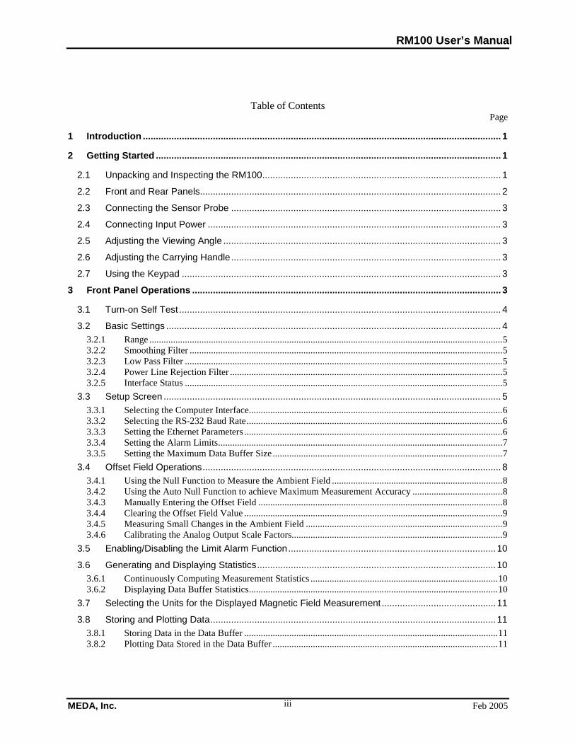
Table of Contents
Page
1 Introduction .......................................................................................................................................... 1
2 Getting Started ..................................................................................................................................... 1
2.1 Unpacking and Inspecting the RM100............................................................................................ 1 2.2 Front and Rear Panels.................................................................................................................... 2 2.3 Connecting the Sensor Probe ........................................................................................................ 3 2.4 Connecting Input Power ................................................................................................................. 3 2.5 Adjusting the Viewing Angle ........................................................................................................... 3 2.6 Adjusting the Carrying Handle ........................................................................................................ 3 2.7 Using the Keypad ........................................................................................................................... 3
3 Front Panel Operations ....................................................................................................................... 3
3.1 Turn-on Self Test ............................................................................................................................ 4 3.2 Basic Settings ................................................................................................................................. 4
3.2.1 Range ..................................................................................................................................................... 5 3.2.2 Smoothing Filter .................................................................................................................................... 5 3.2.3 Low Pass Filter ...................................................................................................................................... 5 3.2.4 Power Line Rejection Filter ................................................................................................................... 5 3.2.5 Interface Status ...................................................................................................................................... 5
3.3 Setup Screen .................................................................................................................................. 5 3.3.1 Selecting the Computer Interface ........................................................................................................... 6 3.3.2 Selecting the RS-232 Baud Rate ............................................................................................................ 6 3.3.3 Setting the Ethernet Parameters ............................................................................................................. 6 3.3.4 Setting the Alarm Limits ........................................................................................................................ 7 3.3.5 Setting the Maximum Data Buffer Size ................................................................................................. 7
3.4 Offset Field Operations ................................................................................................................... 8 3.4.1 Using the Null Function to Measure the Ambient Field ........................................................................ 8 3.4.2 Using the Auto Null Function to achieve Maximum Measurement Accuracy ...................................... 8 3.4.3 Manually Entering the Offset Field ....................................................................................................... 8 3.4.4 Clearing the Offset Field Value ............................................................................................................. 9 3.4.5 Measuring Small Changes in the Ambient Field ................................................................................... 9 3.4.6 Calibrating the Analog Output Scale Factors......................................................................................... 9
3.5 Enabling/Disabling the Limit Alarm Function ................................................................................ 10 3.6 Generating and Displaying Statistics ............................................................................................ 10
3.6.1 Continuously Computing Measurement Statistics ............................................................................... 10 3.6.2 Displaying Data Buffer Statistics ......................................................................................................... 10
3.7 Selecting the Units for the Displayed Magnetic Field Measurement ............................................ 11 3.8 Storing and Plotting Data .............................................................................................................. 11
3.8.1 Storing Data in the Data Buffer ........................................................................................................... 11 3.8.2 Plotting Data Stored in the Data Buffer ............................................................................................... 11
RM100 User’s Manual
Feb 2005 MEDA, Inc. iv
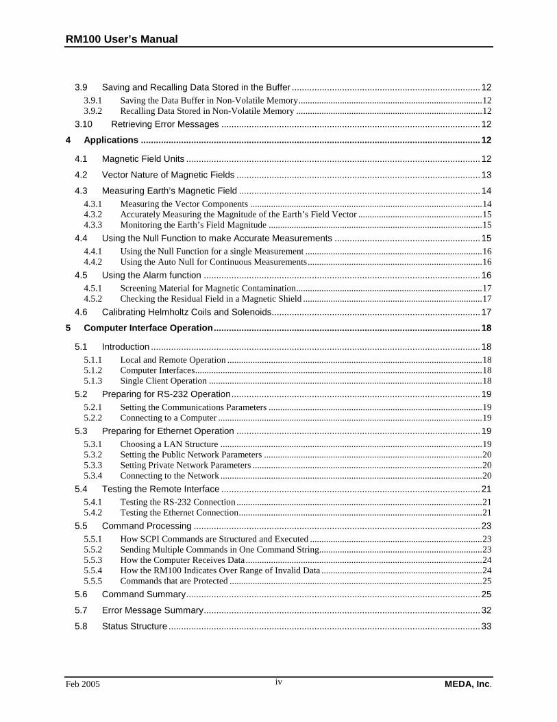
3.9 Saving and Recalling Data Stored in the Buffer ........................................................................... 12 3.9.1 Saving the Data Buffer in Non-Volatile Memory ................................................................................ 12 3.9.2 Recalling Data Stored in Non-Volatile Memory ................................................................................. 12
3.10 Retrieving Error Messages ....................................................................................................... 12 4 Applications ....................................................................................................................................... 12
4.1 Magnetic Field Units ..................................................................................................................... 12 4.2 Vector Nature of Magnetic Fields ................................................................................................. 13 4.3 Measuring Earth’s Magnetic Field ................................................................................................ 14
4.3.1 Measuring the Vector Components ..................................................................................................... 14 4.3.2 Accurately Measuring the Magnitude of the Earth’s Field Vector ...................................................... 15 4.3.3 Monitoring the Earth’s Field Magnitude ............................................................................................. 15
4.4 Using the Null Function to make Accurate Measurements .......................................................... 15 4.4.1 Using the Null Function for a single Measurement ............................................................................. 16 4.4.2 Using the Auto Null for Continuous Measurements ............................................................................ 16
4.5 Using the Alarm function .............................................................................................................. 16 4.5.1 Screening Material for Magnetic Contamination ................................................................................. 17 4.5.2 Checking the Residual Field in a Magnetic Shield .............................................................................. 17
4.6 Calibrating Helmholtz Coils and Solenoids................................................................................... 17 5 Computer Interface Operation .......................................................................................................... 18
5.1 Introduction ................................................................................................................................... 18 5.1.1 Local and Remote Operation ............................................................................................................... 18 5.1.2 Computer Interfaces ............................................................................................................................. 18 5.1.3 Single Client Operation ....................................................................................................................... 18
5.2 Preparing for RS-232 Operation ................................................................................................... 19 5.2.1 Setting the Communications Parameters ............................................................................................. 19 5.2.2 Connecting to a Computer ................................................................................................................... 19
5.3 Preparing for Ethernet Operation ................................................................................................. 19 5.3.1 Choosing a LAN Structure .................................................................................................................. 19 5.3.2 Setting the Public Network Parameters ............................................................................................... 20 5.3.3 Setting Private Network Parameters .................................................................................................... 20 5.3.4 Connecting to the Network .................................................................................................................. 20
5.4 Testing the Remote Interface ....................................................................................................... 21 5.4.1 Testing the RS-232 Connection ........................................................................................................... 21 5.4.2 Testing the Ethernet Connection .......................................................................................................... 21
5.5 Command Processing .................................................................................................................. 23 5.5.1 How SCPI Commands are Structured and Executed ........................................................................... 23 5.5.2 Sending Multiple Commands in One Command String....................................................................... 23 5.5.3 How the Computer Receives Data ....................................................................................................... 24 5.5.4 How the RM100 Indicates Over Range of Invalid Data ...................................................................... 24 5.5.5 Commands that are Protected .............................................................................................................. 25
5.6 Command Summary ..................................................................................................................... 25 5.7 Error Message Summary .............................................................................................................. 32 5.8 Status Structure ............................................................................................................................ 33

RM100 User’s Manual
MEDA, Inc. Feb 2005 v
5.8.1 Status Byte Register ............................................................................................................................. 33 5.8.2 Questionable Event Register ................................................................................................................ 33 5.8.3 Standard Event Status Register ............................................................................................................ 35 5.8.4 Operation Event Register ..................................................................................................................... 35 5.8.5 Clearing the Event and Event Enable Registers ................................................................................... 35
6 Theory of Operation ........................................................................................................................... 36
6.1 Introduction ................................................................................................................................... 36 6.2 Overview ....................................................................................................................................... 36
6.2.1 Embedded Microprocessor .................................................................................................................. 36 6.2.2 User Interface ....................................................................................................................................... 36 6.2.3 Analog Data Filtering and Conversion ................................................................................................ 36
6.3 Fluxgate Magnetometer Theory ................................................................................................... 38 6.3.1 Sensor Construction ............................................................................................................................. 38 6.3.2 Fluxgate Operation .............................................................................................................................. 38 6.3.3 Sensor Signal Processing ..................................................................................................................... 40
6.4 Analog Magnetometer Circuit Configuration ................................................................................ 40 6.4.1 Excitation Circuit ................................................................................................................................. 40 6.4.2 Signal Conditioner ............................................................................................................................... 41 6.4.3 Neutralization Circuit .......................................................................................................................... 41
6.5 Analog Output Filtering ................................................................................................................. 42 7 Maintenance ....................................................................................................................................... 42
7.1 Probe Precautions ........................................................................................................................ 42 7.2 Fuse Replacement ........................................................................................................................ 42 7.3 Calibration Cycle ........................................................................................................................... 42
APPENDIX A SPECIFICATIONS
RM100 User’s Manual
Feb 2005 MEDA, Inc. vi
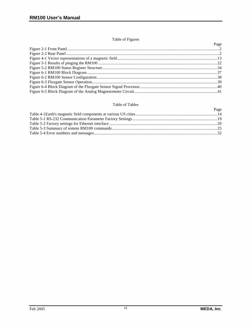
Table of Figures Page
Figure 2-1 Front Panel ................................................................................................................................................... 2 Figure 2-2 Rear Panel .................................................................................................................................................... 2 Figure 4-1 Vector representations of a magnetic field ................................................................................................. 13 Figure 5-1 Results of pinging the RM100 ................................................................................................................... 22 Figure 5-2 RM100 Status Register Structure ............................................................................................................... 34 Figure 6-1 RM100 Block Diagram .............................................................................................................................. 37 Figure 6-2 RM100 Sensor Configuration .................................................................................................................... 38 Figure 6-3 Fluxgate Sensor Operation ......................................................................................................................... 39 Figure 6-4 Block Diagram of the Fluxgate Sensor Signal Processor ........................................................................... 40 Figure 6-5 Block Diagram of the Analog Magnetometer Circuit ................................................................................ 41
Table of Tables Page
Table 4-1Earth's magnetic field components at various US cities ............................................................................... 14 Table 5-1 RS-232 Communication Parameter Factory Settings .................................................................................. 19 Table 5-2 Factory settings for Ethernet interface ........................................................................................................ 20 Table 5-3 Summary of remote RM100 commands ...................................................................................................... 25 Table 5-4 Error numbers and messages ....................................................................................................................... 32

RM100 User’s Manual
MEDA, Inc. Feb 2005 vii
Intentionally left blank


RM100 User’s Manual
MEDA, Inc. Feb 2005 1
1 Introduction The RM100 Nanotesla Meter is a high resolution high accuracy single axis fluxgate magnetometer that can be used to measure static magnetic fields over a range of ±200 µT with a resolution of 0.1 nT. Measurement accuracies of ±0.01% can be achieved over a range of ±100 µT using the neutralizing feature of the RM100.
The RM100 is a replacement for the obsolete Schonstedt Instrument Company HSM-2 Reference Magnetometer that has been the standard instrument used for high accuracy magnetic field measurements over the last thirty years. The RM100 maintains the same accuracy but with the enhanced capabilities afforded by current microprocessor and analog-to-digital converter technology.
Some of the features of the RM100 are:
• 0.1 nT resolution
• ±0.01% basic accuracy traceable to NIST
• 0.5 ppm/ºC stability of the offset field
• ±200 µT measurement range
• One button ambient field cancellation and measurement
• 100, 10, 1, and 0.1 µT analog output ranges for recording and other purposes
• Measurement statistics such as minimum, maximum and average values
• Data storage and on-screen plotting (up to 8,000 samples)
• Remote programming and data acquisition using either RS-232 or Ethernet connections
• SCPI Version 1999.0 compliant remote programming
• National Instruments LabView drivers
• An alarm capability for alerting the user of signals that exceed user-set limits
The RM100 can be used to:
• Screen for magnetic contamination
• Monitor Geomagnetic field variations
• Measure rock magnetism
• Calibrate Helmholtz coils and solenoids used to generate precision fields
• Check shielding effectiveness
• Measure the dipole moments of equipment
• Detect satellite stray fields
2 Getting Started
2.1 Unpacking and Inspecting the RM100 Carefully unpack and inspect the RM100 for physical damage. Verify that the items received agree with the enclosed packing slip. If there are any damaged parts, inform the shipping service and MEDA. If there are any missing parts, contact MEDA.
RM100 User’s Manual
Feb 2005 MEDA, Inc. 2
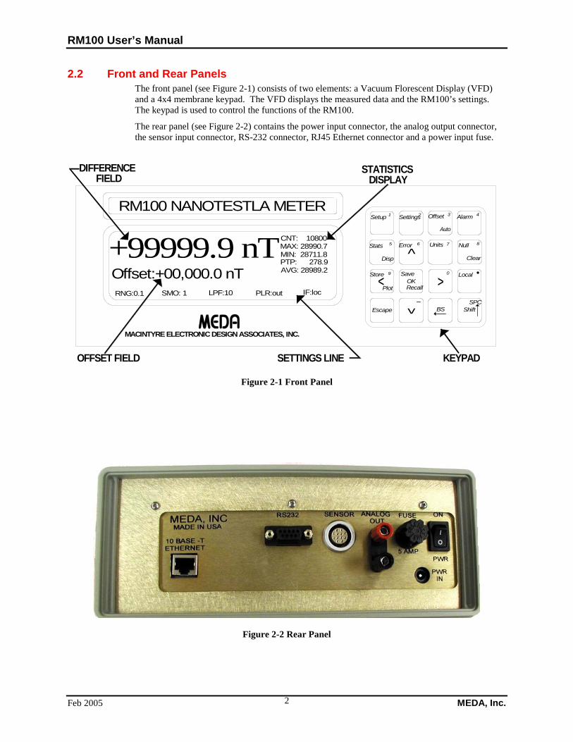
2.2 Front and Rear Panels The front panel (see Figure 2-1) consists of two elements: a Vacuum Florescent Display (VFD) and a 4x4 membrane keypad. The VFD displays the measured data and the RM100’s settings. The keypad is used to control the functions of the RM100.
The rear panel (see Figure 2-2) contains the power input connector, the analog output connector, the sensor input connector, RS-232 connector, RJ45 Ethernet connector and a power input fuse.
DIFFERENCE
FIELD
OFFSET FIELD SETTINGS LINE KEYPAD
STATISTICSDISPLAY
Auto
MACINTYRE ELECTRONIC DESIGN ASSOCIATES, INC.
RM100 NANOTESTLA METERSettings OffsetSetup 1 Alarm2 3 4
Stats Units Null5 6 7 8
^
^
^ ^9 0
OK
BS ShiftSPC
Disp
Error
Clear
Store
Recall
Local
Plot
Escape
Save
RNG:0.1 SMO: 1 LPF:10 PLR:out IF:loc
Offset:+00,000.0 nT+99999.9 nTCNT: 10800
MAX: 28990.7MIN: 28711.8PTP: 278.9AVG: 28989.2
Figure 2-1 Front Panel
Figure 2-2 Rear Panel

RM100 User’s Manual
MEDA, Inc. Feb 2005 3
2.3 Connecting the Sensor Probe The RM100 sensor probe connects to the RM100 through a 50’ cable. Connect the sensor cable to the sensor input connector on the rear panel of the RM100.
The sensor must be connected to the RM100 before turning power ON.
2.4 Connecting Input Power The RM100 input power is supplied using an external 7.5 VDC power adaptor. The power adaptor will operate from power line voltages of 100 to 240 VAC and frequencies of 60/50 Hz. The standard power cord supplied with the RM100 fits North American power outlets. Other power cords are available for non-North American use.
Plug the power adaptor into the power line outlet. With the RM100 power switch in the OFF position insert the adaptor output into the RM100 power input connector. Set the RM100 power switch to ON to apply power to the RM100.
2.5 Adjusting the Viewing Angle The RM100 is equipped with two legs on the bottom near the front that can be rotated into the vertical position to tilt the front of the meter up slightly. The carrying handle attached to the left side of the case can be rotated downward and under the RM100 to achieve a greater viewing angle. Pull the handle along the direction indicated by the handle arrow on the left side of the case until it becomes disengaged. Rotate the handle clockwise until it is below the bottom of the case then release the side connection until it reengages.
2.6 Adjusting the Carrying Handle The RM100 carrying handle can be placed into two positions for carrying. The handle can be locked in place above the case or in front of the case. To move the handle, disengage it from the left side connection, rotate it until it is in the desired position, then reengage the handle connection.
2.7 Using the Keypad All local operations are controlled using the 4x4 keypad on the right hand side of the front panel. The keypad is constructed of membrane switches with tactile feedback. There is also audio acknowledgement when a key has been pressed and recognized by the RM100. Some keys, such as the Shift key, cause an annunciator to be activated. The annunciator will appear between the Offset display in the middle of the front panel screen and the settings line at the bottom of the screen.
The word in the upper left corner of each key indicates the key’s main function. The word in the lower right corner of each key indicates the key’s second function which is activated by pressing the Shift key.
3 Front Panel Operations This section describes how to operate the RM100 using the front panel controls. Refer to Section 5 for an explanation of how to remotely control the RM100 using an RS-232 or Ethernet connection. When the RM100 is first turned on the following message will appear on the front panel display:
FTP server active for firmware update—hit key to continue
The RM100 has a built in FTP server that is used for updating the firmware. The FTP server can be terminated and the RM100 stated up immediately by pressing a key on the keypad. The RM100
RM100 User’s Manual
Feb 2005 MEDA, Inc. 4
will automatically start up after 60 seconds of no network or keyboard activity. Section 7 describes how to use this capability to upgrade the firmware.
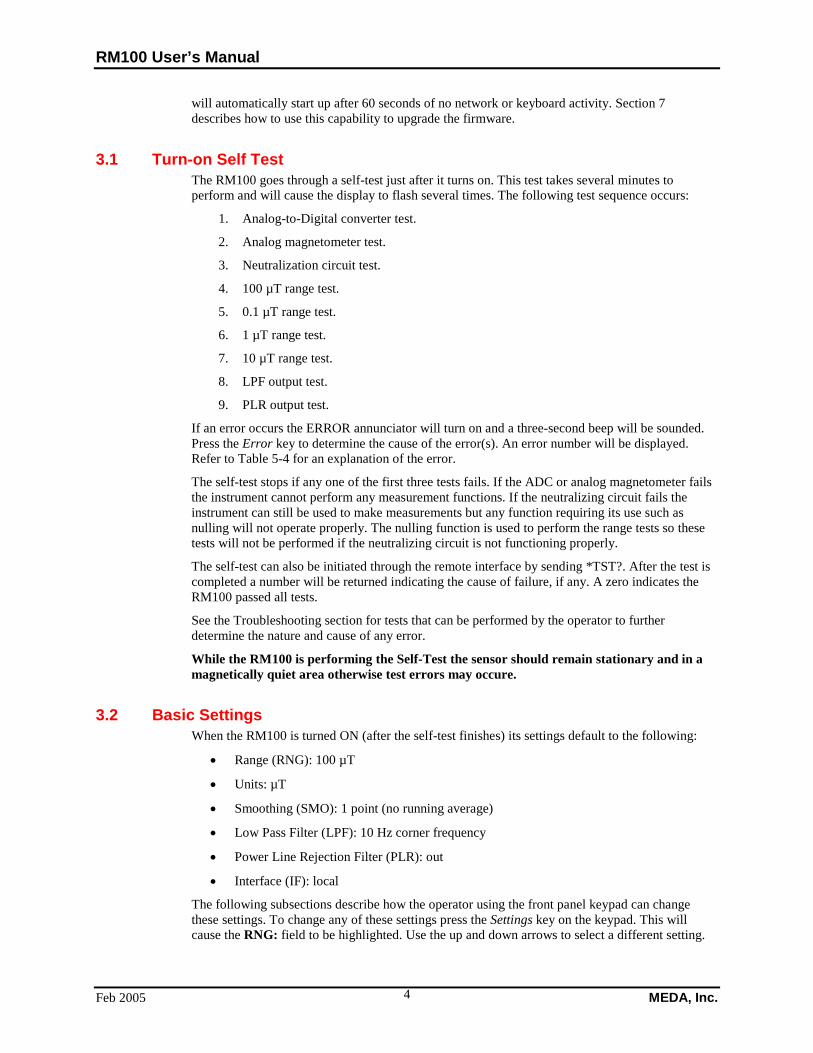
3.1 Turn-on Self Test The RM100 goes through a self-test just after it turns on. This test takes several minutes to perform and will cause the display to flash several times. The following test sequence occurs:
1. Analog-to-Digital converter test.
2. Analog magnetometer test.
3. Neutralization circuit test.
4. 100 µT range test.
5. 0.1 µT range test.
6. 1 µT range test.
7. 10 µT range test.
8. LPF output test.
9. PLR output test.
If an error occurs the ERROR annunciator will turn on and a three-second beep will be sounded. Press the Error key to determine the cause of the error(s). An error number will be displayed. Refer to Table 5-4 for an explanation of the error.
The self-test stops if any one of the first three tests fails. If the ADC or analog magnetometer fails the instrument cannot perform any measurement functions. If the neutralizing circuit fails the instrument can still be used to make measurements but any function requiring its use such as nulling will not operate properly. The nulling function is used to perform the range tests so these tests will not be performed if the neutralizing circuit is not functioning properly.
The self-test can also be initiated through the remote interface by sending *TST?. After the test is completed a number will be returned indicating the cause of failure, if any. A zero indicates the RM100 passed all tests.
See the Troubleshooting section for tests that can be performed by the operator to further determine the nature and cause of any error.
While the RM100 is performing the Self-Test the sensor should remain stationary and in a magnetically quiet area otherwise test errors may occure.
3.2 Basic Settings When the RM100 is turned ON (after the self-test finishes) its settings default to the following:
• Range (RNG): 100 µT
• Units: µT
• Smoothing (SMO): 1 point (no running average)
• Low Pass Filter (LPF): 10 Hz corner frequency
• Power Line Rejection Filter (PLR): out
• Interface (IF): local
The following subsections describe how the operator using the front panel keypad can change these settings. To change any of these settings press the Settings key on the keypad. This will cause the RNG: field to be highlighted. Use the up and down arrows to select a different setting.
RM100 User’s Manual
MEDA, Inc. Feb 2005 5
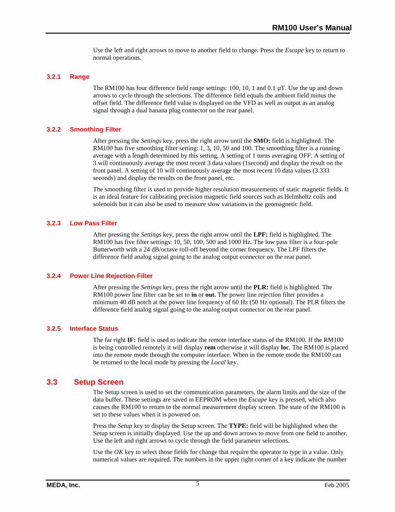
Use the left and right arrows to move to another field to change. Press the Escape key to return to normal operations.
3.2.1 Range The RM100 has four difference field range settings: 100, 10, 1 and 0.1 µT. Use the up and down arrows to cycle through the selections. The difference field equals the ambient field minus the offset field. The difference field value is displayed on the VFD as well as output as an analog signal through a dual banana plug connector on the rear panel.
3.2.2 Smoothing Filter After pressing the Settings key, press the right arrow until the SMO: field is highlighted. The RM100 has five smoothing filter setting: 1, 3, 10, 50 and 100. The smoothing filter is a running average with a length determined by this setting. A setting of 1 turns averaging OFF. A setting of 3 will continuously average the most recent 3 data values (1second) and display the result on the front panel. A setting of 10 will continuously average the most recent 10 data values (3.333 seconds) and display the results on the front panel, etc.
The smoothing filter is used to provide higher resolution measurements of static magnetic fields. It is an ideal feature for calibrating precision magnetic field sources such as Helmholtz coils and solenoids but it can also be used to measure slow variations in the geomagnetic field.
3.2.3 Low Pass Filter After pressing the Settings key, press the right arrow until the LPF: field is highlighted. The RM100 has five filter settings: 10, 50, 100, 500 and 1000 Hz. The low pass filter is a four-pole Butterworth with a 24 dB/octave roll-off beyond the corner frequency. The LPF filters the difference field analog signal going to the analog output connector on the rear panel.
3.2.4 Power Line Rejection Filter After pressing the Settings key, press the right arrow until the PLR: field is highlighted. The RM100 power line filter can be set to in or out. The power line rejection filter provides a minimum 40 dB notch at the power line frequency of 60 Hz (50 Hz optional). The PLR filters the difference field analog signal going to the analog output connector on the rear panel.
3.2.5 Interface Status The far right IF: field is used to indicate the remote interface status of the RM100. If the RM100 is being controlled remotely it will display rem otherwise it will display loc. The RM100 is placed into the remote mode through the computer interface. When in the remote mode the RM100 can be returned to the local mode by pressing the Local key.
3.3 Setup Screen The Setup screen is used to set the communication parameters, the alarm limits and the size of the data buffer. These settings are saved in EEPROM when the Escape key is pressed, which also causes the RM100 to return to the normal measurement display screen. The state of the RM100 is set to these values when it is powered on.
Press the Setup key to display the Setup screen. The TYPE: field will be highlighted when the Setup screen is initially displayed. Use the up and down arrows to move from one field to another. Use the left and right arrows to cycle through the field parameter selections.
Use the OK key to select those fields for change that require the operator to type in a value. Only numerical values are required. The numbers in the upper right corner of a key indicate the number

RM100 User’s Manual
Feb 2005 MEDA, Inc. 6
that will be typed in when it is pressed during data entry. Press the OK key after entering data into a field to indicate acceptance of the new value. Press the Escape key to reject the entered value and return to the original value.
The following subsections describe how to change each setting.
3.3.1 Selecting the Computer Interface A computer through either an RS-232 serial connection or an Ethernet connection can control the RM100 remotely. With the TYPE: field highlighted use the left or right arrow to select between serial (RS-232) and Ether (Ethernet) interface modes.
3.3.2 Selecting the RS-232 Baud Rate The operator can set the baud rate of the RS-232 port to one of five values: 9600, 19200, 38400, 57600 or 115200. With the BAUD: field highlighted use the left or right arrow to cycle through the allowed baud rates. The default baud rate is 9600.
3.3.3 Setting the Ethernet Parameters The Ethernet connection uses the TCP/IP protocol. The RM100 requires a static IP address, network mask, gateway (router) address, and port number to communicate over the network. Initially these parameters are set to default values that are meant for a private network (one not connected to the Internet). The user must set these parameters to the values appropriate for his or her network. These values are usually obtained from the Network Administrator.
To set the IP address:
• Highlight the IP: field.
• Press the OK key. This will erase the current value and place a cursor at the beginning of the field.
• Type in the new IP address in dot decimal notation (e.g. 192.168.0.2). If you make a mistake, press the BS key to erase the last entry and move back one space.
• Press OK to accept the new value or Escape to return to the original value.
To set the MASK address:
• Highlight the MASK: field.
• Press the OK key. This will erase the current value and place a cursor at the beginning of the field.
• Type in the new Mask address in dot decimal notation (e.g. 255.255.255.0). If you make a mistake, press the BS key to erase the last entry and move back one space.
• Press OK to accept the new value or Escape to return to the original value.
To set the GATE address:
• Highlight the GATE: field.
• Press the OK key. This will erase the current value and place a cursor at the beginning of the field.
• Type in the new gateway (router) address in dot decimal notation (e.g. 192.168.0.1). If you make a mistake, press the BS key to erase the last entry and move back one space.
• Press OK to accept the new value or Escape to return to the original value.
To set the PORT value:

RM100 User’s Manual
MEDA, Inc. Feb 2005 7
• Highlight the PORT: field.
• Press the OK key. This will erase the current value and place a cursor at the beginning of the field.
• Type in the new port value (the default port is 20001). The port value must be between 0 and 65536. If you make a mistake, press the BS key to erase the last entry and move back one space.
• Press OK to accept the new value or Escape to return to the original value.
3.3.4 Setting the Alarm Limits The operator can set minimum and maximum alarm limits from -99999 nT to 99999 nT. The maximum alarm limit must be greater than the minimum alarm limit. When the alarm is armed the current measurement is compared to these limits and the alarm is activated while the current measurement remains outside of these limits. The default MIN and MAX limits are -5 nT and +5 nT respectively.
To set the minimum alarm limit:
• Highlight the MIN: field.
• Press the OK key. This will erase the current value and place a cursor at the beginning of the field.
• Type in the new minimum alarm limit. If you make a mistake, press the BS key to erase the last entry and move back one space.
• Press OK to accept the new value or Escape to return to the original value.
To set the maximum alarm limit:
• Highlight the MAX: field.
• Press the OK key. This will erase the current value and place a cursor at the beginning of the field.
• Type in the new maximum alarm limit. If you make a mistake, press the BS key to erase the last entry and move back one space.
• Press OK to accept the new value or Escape to return to the original value.
3.3.5 Setting the Maximum Data Buffer Size The maximum data buffer size determines how much data can be stored using the Store function. The default value is 1024 points. This represents 341 seconds of data at 3 samples per second. The maximum buffer size can be increased to 16,384 points (91 minutes) or reduced to 1 point.
To set the maximum data buffer size:
• Highlight the SIZE: field.
• Press the OK key. This will erase the current value and place a cursor at the beginning of the field.
• Type in the new maximum data buffer size. If you make a mistake, press the BS key to erase the last entry and move back one space.
• Press OK to accept the new value or Escape to return to the original value.

RM100 User’s Manual
Feb 2005 MEDA, Inc. 8
3.4 Offset Field Operations The RM100 sensor is surrounded by a solenoid that is used to generate an offset field. The RM100 sensor measures the difference between the ambient field at the sensor and the offset field produced by the solenoid. The offset field is very accurate and its accuracy is traceable to NIST.
The offset field function can be used to:
• Accurately measure a static magnetic field.
• Null (neutralize) the ambient field so that small changes in the field can be measured accurately.
• Calibrate the analog output scale factors.
• Measure fields up to ±200 µT.
3.4.1 Using the Null Function to Measure the Ambient Field The ambient field component along the sensitive axis of the sensor can be measured accurately by pressing the Null key. The RM100 will automatically apply an offset field that will null the ambient field. The value of the nulling (neutralizing) field, which is displayed in the Offset: field in the middle of the screen, is the negative of the value of the ambient field. The value of the offset field has an accuracy of ±0.01% of the reading ±0.2 nT. The offset field has a minimum step size of 0.38 nT.
After the field is initially nulled, the main measurement field displays the difference between the ambient field and the neutralizing field, and the RM100 is set to the 0.1 µT range.
3.4.2 Using the Auto Null Function to achieve Maximum Measurement Accuracy The ambient field component along the sensitive axis of the sensor can be measured continuously at the highest accuracy by using the Auto Null feature. This function is activated by pressing the Shift key followed by the Offset key. In the Auto Null mode the RM100 continuously updates the offset field whenever the ambient field changes by more than 1.1 nT and the magnetic field value (-offset field + difference field) is displayed instead of the difference field.
This mode of operation provides the highest measurement accuracy. The Limit Alarm function is disabled when the RM100 is in the Auto Null mode. Also the analog output is not usable in this mode since it is continuously zeroed.
In the Auto Null mode the RM100 can accommodate changes up to a rate of 300 nT per second. If the field should change by 100 nT the RM100 will automatically perform the Null function as if the Null key had been pressed.
The Auto Null function is only effective for fields up to ±100 µT. To measure fields greater than ±100 µT use the standard Null function.
3.4.3 Manually Entering the Offset Field The user can manually enter an offset field of any value from +99,999.9 nT to –99,999.9 nT.
To manually enter an offset field:
• Press the Offset key. The polarity position of the Offset: field will be highlighted.
• Use the up and down arrows to change the polarity of the offset field or to turn the field OFF (blank polarity position).
• Use the left and right arrows to move the cursor to one of the numerical fields.
• Use the up and down arrows to change the value of the numerical field.

RM100 User’s Manual
MEDA, Inc. Feb 2005 9
• Press the Escape key to exit the offset value entry and return to normal operations.
The offset field minimum step size is 0.381 nT. When entering values in the 0.1 nT field the actual offset field will change only for 0.4 and 0.8 nT entries.
The Offset keys are inhibited when the RM100 is in the Auto Null mode.
3.4.4 Clearing the Offset Field Value The offset field can be cleared (set to zero value and turned OFF) by pressing the Shift key followed by the Null key. This will change the RM100 to the 100 µT range and the difference field displayed on the screen will be the current value of the ambient field.
3.4.5 Measuring Small Changes in the Ambient Field Use the Null function to accurately measure small changes in the ambient field. The analog output or the Store function can be used to record the changes.
To measure small changes in the ambient field
• Press the Null key to null the ambient field. Record the value of the offset field, which is the negative value of the measured ambient field.
• Press the Settings key and use the up or down arrows to change the range to the desired value based on the expected change in the ambient field.
• Press the Escape key to return to normal operation.
• Attach the analog output to a recording device and/or press the Store key.
The basic accuracy of the analog output scale factor is ±1%. For better accuracy use the procedure in section 3.4.6 to calibrate the analog output scale factor before using the analog output to record changes.
3.4.6 Calibrating the Analog Output Scale Factors The analog output scale factors for each of the four ranges can be accurately calibrated by using the offset function to generate a very accurate magnetic field. The following procedure should be performed in a magnetically quiet area where the measurements will not be disturbed by moving ferromagnetic objects. The measurements should be performed as quickly as practical since the Geomagnetic field is constantly changing and could affect the accuracy of the calibration.
To calibrate the scale factor of the analog output
• Reset the offset field by pressing the Shift key followed by the Clear key.
• With the sensitive axis of the sensor in the horizontal plane point the sensor east and rotate it slowly in the horizontal plane until the measured field is less than 10 nT.
• Secure the sensor so that it doesn’t move.
• Press the Settings key and use the up or down arrows to select the analog output range to calibrate.
• Press the Offset key to highlight the polarity position of the Offset: field. The polarity position should be blank and the value of the offset field should be zero.
• Use the right arrow to move to the digit position representing the full-scale field for the selected range (e.g. if the range is 0.1 µT then go to the 100 nT position).
• Use the up or down arrow to set the offset field value to the full-scale value of the range being calibrated.

RM100 User’s Manual
Feb 2005 MEDA, Inc. 10
• Use the left arrow to return to the polarity position.
• Press the up arrow to change the polarity of the offset field to + and record the analog output voltage.
• Press the up arrow again to change the polarity of the offset field to – and record the analog output voltage.
• Compute the scale factor using the following equation: ( ) nTvolts
HRRSF /
2 ⋅−
= −+
where +R is the analog output voltage recorded for the positive offset field, −R is the analog output voltage recorded for the negative offset field and H is the value of the offset field.
When calibrating the 100 µT range use a 99,999 nT offset field since there is no 100,000 nT offset field position.
3.5 Enabling/Disabling the Limit Alarm Function The limit alarm function limits are set using the Setup screen (see section 3.3.4). The alarm is initially disabled. Press the Alarm key to enable the alarm. The Al annunciator will be displayed when the alarm is enabled. Press the Alarm key again to disable the alarm. When the alarm is enabled the alarm will sound and remain active whenever the difference field is outside the specified limits. The difference field equals the ambient field minus the offset field.
Before activating the alarm use the Null function to cancel the ambient field. The limit alarm function is disabled if the RM100 is in the Auto Null mode.
3.6 Generating and Displaying Statistics Measurement statistics can be computed continuously while measurements are being made or just on the data in the data buffer.
3.6.1 Continuously Computing Measurement Statistics The RM100 can compute the measurement statistics on an unlimited number of data points. Only the statistics are retained not the actual measurements upon which the statistics are based.
Press the Stats key to start continuous computation of measurement statistics. The Stats annunciator is displayed, the statistics variables are initialized and statistics on all future measurements begins. Pressing the Stats key a second time stops the collection of measurement statistics, turns off the Stats annunciator and clears all statistics variable.
Press the Shift key followed by the Stats key to display the current values of the measurement statistics. These values will be displayed in the upper right corner of the screen. Repeat these keystrokes to remove the measurement statistics from the screen. The measurement statistics can only be displayed while the Stats annunciator is displayed.
3.6.2 Displaying Data Buffer Statistics Measurement statistics on the data in the data buffer can be displayed whenever the Stats annunciator is off. Press the Shift key followed by the Stats key to display the data buffer measurement statistics. These values will be displayed in the upper right corner of the screen. Repeat these keystrokes to remove the data buffer measurement statistics from the screen.
Data storage is suspended while the statistics are being computed and displayed. It is best to wait until the data buffer is full before displaying the measurement statistics.
RM100 User’s Manual
MEDA, Inc. Feb 2005 11
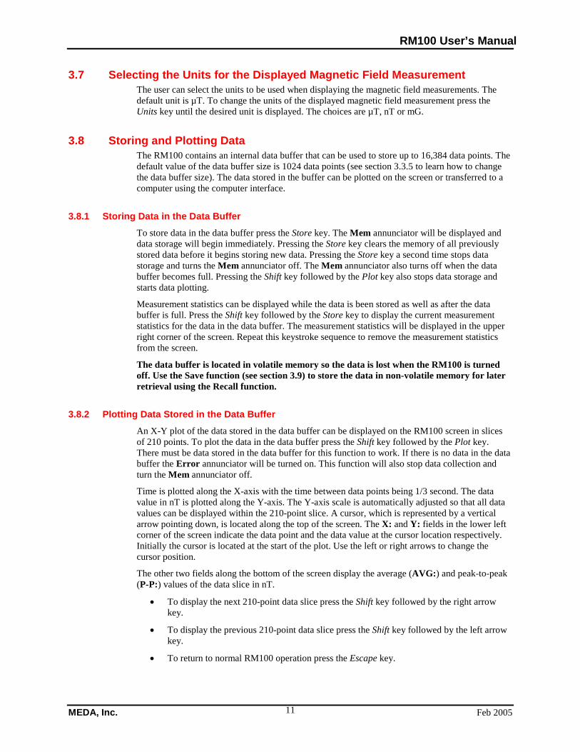
3.7 Selecting the Units for the Displayed Magnetic Field Measurement The user can select the units to be used when displaying the magnetic field measurements. The default unit is µT. To change the units of the displayed magnetic field measurement press the Units key until the desired unit is displayed. The choices are µT, nT or mG.
3.8 Storing and Plotting Data The RM100 contains an internal data buffer that can be used to store up to 16,384 data points. The default value of the data buffer size is 1024 data points (see section 3.3.5 to learn how to change the data buffer size). The data stored in the buffer can be plotted on the screen or transferred to a computer using the computer interface.
3.8.1 Storing Data in the Data Buffer To store data in the data buffer press the Store key. The Mem annunciator will be displayed and data storage will begin immediately. Pressing the Store key clears the memory of all previously stored data before it begins storing new data. Pressing the Store key a second time stops data storage and turns the Mem annunciator off. The Mem annunciator also turns off when the data buffer becomes full. Pressing the Shift key followed by the Plot key also stops data storage and starts data plotting.
Measurement statistics can be displayed while the data is been stored as well as after the data buffer is full. Press the Shift key followed by the Store key to display the current measurement statistics for the data in the data buffer. The measurement statistics will be displayed in the upper right corner of the screen. Repeat this keystroke sequence to remove the measurement statistics from the screen.
The data buffer is located in volatile memory so the data is lost when the RM100 is turned off. Use the Save function (see section 3.9) to store the data in non-volatile memory for later retrieval using the Recall function.
3.8.2 Plotting Data Stored in the Data Buffer An X-Y plot of the data stored in the data buffer can be displayed on the RM100 screen in slices of 210 points. To plot the data in the data buffer press the Shift key followed by the Plot key. There must be data stored in the data buffer for this function to work. If there is no data in the data buffer the Error annunciator will be turned on. This function will also stop data collection and turn the Mem annunciator off.
Time is plotted along the X-axis with the time between data points being 1/3 second. The data value in nT is plotted along the Y-axis. The Y-axis scale is automatically adjusted so that all data values can be displayed within the 210-point slice. A cursor, which is represented by a vertical arrow pointing down, is located along the top of the screen. The X: and Y: fields in the lower left corner of the screen indicate the data point and the data value at the cursor location respectively. Initially the cursor is located at the start of the plot. Use the left or right arrows to change the cursor position.
The other two fields along the bottom of the screen display the average (AVG:) and peak-to-peak (P-P:) values of the data slice in nT.
• To display the next 210-point data slice press the Shift key followed by the right arrow key.
• To display the previous 210-point data slice press the Shift key followed by the left arrow key.
• To return to normal RM100 operation press the Escape key.
RM100 User’s Manual
Feb 2005 MEDA, Inc. 12
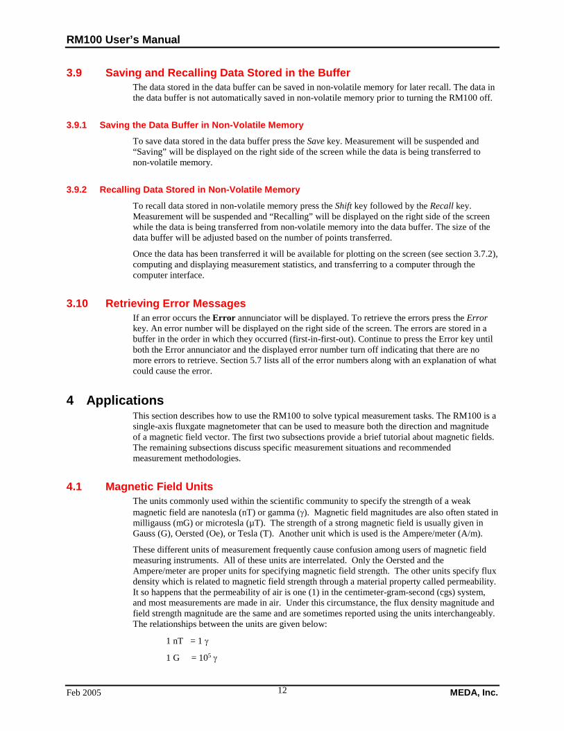
3.9 Saving and Recalling Data Stored in the Buffer The data stored in the data buffer can be saved in non-volatile memory for later recall. The data in the data buffer is not automatically saved in non-volatile memory prior to turning the RM100 off.
3.9.1 Saving the Data Buffer in Non-Volatile Memory To save data stored in the data buffer press the Save key. Measurement will be suspended and “Saving” will be displayed on the right side of the screen while the data is being transferred to non-volatile memory.
3.9.2 Recalling Data Stored in Non-Volatile Memory To recall data stored in non-volatile memory press the Shift key followed by the Recall key. Measurement will be suspended and “Recalling” will be displayed on the right side of the screen while the data is being transferred from non-volatile memory into the data buffer. The size of the data buffer will be adjusted based on the number of points transferred.
Once the data has been transferred it will be available for plotting on the screen (see section 3.7.2), computing and displaying measurement statistics, and transferring to a computer through the computer interface.
3.10 Retrieving Error Messages If an error occurs the Error annunciator will be displayed. To retrieve the errors press the Error key. An error number will be displayed on the right side of the screen. The errors are stored in a buffer in the order in which they occurred (first-in-first-out). Continue to press the Error key until both the Error annunciator and the displayed error number turn off indicating that there are no more errors to retrieve. Section 5.7 lists all of the error numbers along with an explanation of what could cause the error.
4 Applications This section describes how to use the RM100 to solve typical measurement tasks. The RM100 is a single-axis fluxgate magnetometer that can be used to measure both the direction and magnitude of a magnetic field vector. The first two subsections provide a brief tutorial about magnetic fields. The remaining subsections discuss specific measurement situations and recommended measurement methodologies.
4.1 Magnetic Field Units The units commonly used within the scientific community to specify the strength of a weak magnetic field are nanotesla (nT) or gamma (γ). Magnetic field magnitudes are also often stated in milligauss (mG) or microtesla (µT). The strength of a strong magnetic field is usually given in Gauss (G), Oersted (Oe), or Tesla (T). Another unit which is used is the Ampere/meter (A/m).
These different units of measurement frequently cause confusion among users of magnetic field measuring instruments. All of these units are interrelated. Only the Oersted and the Ampere/meter are proper units for specifying magnetic field strength. The other units specify flux density which is related to magnetic field strength through a material property called permeability. It so happens that the permeability of air is one (1) in the centimeter-gram-second (cgs) system, and most measurements are made in air. Under this circumstance, the flux density magnitude and field strength magnitude are the same and are sometimes reported using the units interchangeably. The relationships between the units are given below:
1 nT = 1 γ
1 G = 105 γ

RM100 User’s Manual
MEDA, Inc. Feb 2005 13
1 A/m = 4π x 10-3 Oe
1 T = 104 G
1mG = 0.1 µT
The RM100 allows the user to select nT, µT or mG as the unit of magnetic field strength to display.
4.2 Vector Nature of Magnetic Fields Magnetic fields are vectors. At any point in space a magnetic field has a magnitude and a direction. This is illustrated in Fig. 4-1.
zR
y
x
H
Z
Y
XD
I
Figure 4-1 Vector representations of a magnetic field
A vector is usually represented graphically by an arrow which indicates the direction of the vector and has a length which is proportional to the vector magnitude. A magnetic field vector can be separated into three vector components (X,Y,Z) which are at right angles to one another. These are called the rectangular components of the vector. The magnitude (R) of the vector is determined by squaring the component vector magnitudes, summing the squares and then taking the square root of the sum. The magnetic field vector can also be represented in polar coordinates by two angles (I and D) and a magnitude (R). In Fig. 4-1 H is the component of the magnetic field vector in the X-Y plane, which is usually chosen to be the horizontal plane.
The rectangular and polar components of the vector are related to one another. Use the following equations to convert from one set of components to the other:
( )( )
( )( )HZI
XYD
ZYXR
YXH
IRZDHYDHX
1
1
222
22
tantan
sinsincos
−
−
=
=
++=
+=
⋅=⋅=⋅=
The following subsection describes how the RM100 can be used to measure the vector components in either of these two coordinate system representations.

RM100 User’s Manual
Feb 2005 MEDA, Inc. 14
4.3 Measuring Earth’s Magnetic Field We are immersed in a static magnetic field produced by the Earth. The presence of this field both helps us and hinders us in the measurement of magnetic fields. We are all familiar with compasses. The compass needle is itself a magnet and, when placed in Earth's magnetic field, it points toward the north magnetic pole which coincidentally is very near the geographic North Pole. This is a useful property of the Earth's field since it allows us to orient ourselves everywhere on Earth except at the poles themselves.
4.3.1 Measuring the Vector Components The compass needle only provides us with directional information about the vector pointing to the magnetic north pole. The RM100 can be used to measure both the direction and magnitude of the Earth’s field vector as well as its North-South, East-West, and vertical vector components. Follow the steps described below. Make sure you are outside and at least twenty feet away from any magnetic object (anything made from iron or steel).
1. Tape a piece of paper to a level surface made from non-magnetic material. Place the probe on the paper.
2. Set the RM100 on the 100 µT range and rotate the probe for a zero reading. Reduce the range to 0.1µT and fine tune the angular position by rotating the sensor for the lowest reading possible.
3. Draw a straight line on the paper along the edge of the probe.
4. Use a protractor or right angle triangle to draw a line at 90 degrees to the first line. Align the probe edge along this line with the probe arrow pointing approximately north, press the Null key, and record the RM100 offset reading. This is the negative value of the horizontal component (H) of the Earth’s field.
5. Orient the probe in the vertical direction with the end flat against the surface where the two lines cross. Press the Null key and record the RM100 offset reading. This is the vertical component (Z) of Earth’s field.
6. Compute the total field magnitude 22 ZHR += .
7. Compute the inclination of the field ( )HZI arctan= radians.
The first line drawn on the paper is the East-West direction. The second line is the North-South direction. The Inclination angle is the angle between the Earth’s magnetic field vector and the horizontal plane. A positive reading when measuring H indicates the direction of the north magnetic pole.
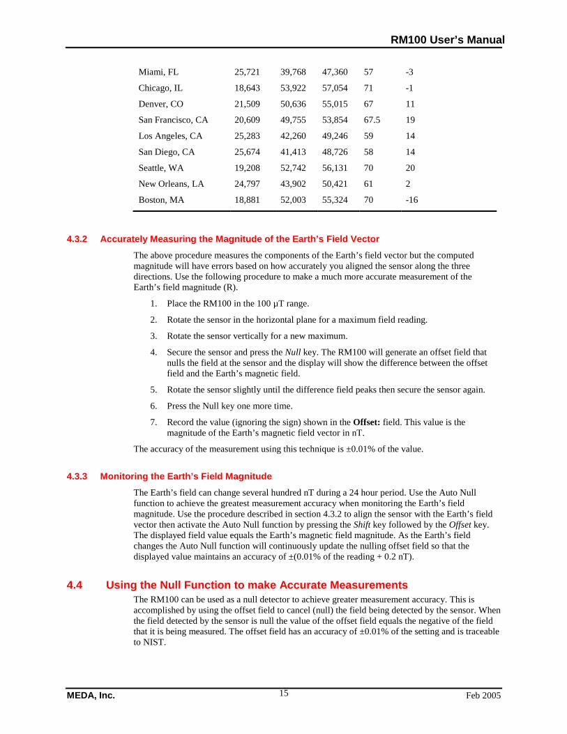
Table 4-1lists the approximate values of I, H, Z, R and magnetic declination for several U.S. cities. This data was determined by using a computer model available from the U.S. Department of Commerce. The magnetic declination is the angular deviation of the magnetic North with the geodetic North. If the sign is positive then the geodetic North is west of the Magnetic north. If it is negative then it is east of the Magnetic north.
Table 4-1Earth's magnetic field components at various US cities
City H (nT) Z (nT) R (nT) I (deg) Declination (deg)
Washington, D. C. 20,535 49,866 53,929 67 -13
New York, NY 19,508 51,553 55,121 69 -13
RM100 User’s Manual
MEDA, Inc. Feb 2005 15
Miami, FL 25,721 39,768 47,360 57 -3
Chicago, IL 18,643 53,922 57,054 71 -1
Denver, CO 21,509 50,636 55,015 67 11
San Francisco, CA 20,609 49,755 53,854 67.5 19
Los Angeles, CA 25,283 42,260 49,246 59 14
San Diego, CA 25,674 41,413 48,726 58 14
Seattle, WA 19,208 52,742 56,131 70 20
New Orleans, LA 24,797 43,902 50,421 61 2
Boston, MA 18,881 52,003 55,324 70 -16
4.3.2 Accurately Measuring the Magnitude of the Earth’s Field Vector The above procedure measures the components of the Earth’s field vector but the computed magnitude will have errors based on how accurately you aligned the sensor along the three directions. Use the following procedure to make a much more accurate measurement of the Earth’s field magnitude (R).
1. Place the RM100 in the 100 µT range.
2. Rotate the sensor in the horizontal plane for a maximum field reading.
3. Rotate the sensor vertically for a new maximum.
4. Secure the sensor and press the Null key. The RM100 will generate an offset field that nulls the field at the sensor and the display will show the difference between the offset field and the Earth’s magnetic field.
5. Rotate the sensor slightly until the difference field peaks then secure the sensor again.
6. Press the Null key one more time.
7. Record the value (ignoring the sign) shown in the Offset: field. This value is the magnitude of the Earth’s magnetic field vector in nT.
The accuracy of the measurement using this technique is ±0.01% of the value.
4.3.3 Monitoring the Earth’s Field Magnitude The Earth’s field can change several hundred nT during a 24 hour period. Use the Auto Null function to achieve the greatest measurement accuracy when monitoring the Earth’s field magnitude. Use the procedure described in section 4.3.2 to align the sensor with the Earth’s field vector then activate the Auto Null function by pressing the Shift key followed by the Offset key. The displayed field value equals the Earth’s magnetic field magnitude. As the Earth’s field changes the Auto Null function will continuously update the nulling offset field so that the displayed value maintains an accuracy of ±(0.01% of the reading + 0.2 nT).
4.4 Using the Null Function to make Accurate Measurements The RM100 can be used as a null detector to achieve greater measurement accuracy. This is accomplished by using the offset field to cancel (null) the field being detected by the sensor. When the field detected by the sensor is null the value of the offset field equals the negative of the field that it is being measured. The offset field has an accuracy of ±0.01% of the setting and is traceable to NIST.

RM100 User’s Manual
Feb 2005 MEDA, Inc. 16
4.4.1 Using the Null Function for a single Measurement The Null keypad function accomplishes this task automatically. When the Null key is pressed the following actions take place:
1. The range is set to 100 µT and smoothing is turned off.
2. The offset field is set to zero.
3. The ambient field is measured and then the offset field is set to minus the ambient field.
4. The range is changed to 1 µT.
5. The difference between the ambient field and the offset field is measured.
6. The offset field is trimmed based on the difference field measurement.
7. The range is changed to 0.1 µT and steps 5 and 6 are repeated.
This whole process takes about 3 seconds. Unless the field is changing rapidly the null field should now be under 1 nT. The actual field can be determined using the following equation:
Actual field = - (offset field) + (difference field).
The difference field accuracy is ±(1% of the reading +1 nT) therefore the accuracy of the actual field is ±(0.01% of the offset field + 1% of the difference field + 1 nT).
4.4.2 Using the Auto Null for Continuous Measurements Use the Auto Null function to achieve the highest accuracy when making continuous measurements of a DC or slowly changing magnetic field. The Auto Null function measures the difference between the ambient field and the nulling offset field three times per second. The offset field is updated whenever the difference is more than 1.1 nT. The displayed value is the negative of the offset field + the difference field. The accuracy of the displayed field measurement is ±(0.01% of the reading + 0.2 nT). Use the following procedure to make the measurements:
1. Align the sensor in the desired direction and secure it.
2. Press the Shift key followed by the Offset key.
The RM100 will first null the field and then go into the Auto Null mode. The value displayed will be the measured magnetic field instead of the difference field. The magnitude of the field should be within 1 nT of the offset field.
In the Auto Null mode the RM100 can accommodate changes up to a rate of 300 nT per second. If the field should change by 100 nT the RM100 will automatically perform the Null function as if the Null key had been pressed.
The Auto Null function is only effective for fields up to ±100 µT. To measure fields greater than ±100 µT use the standard Null function.
You can use the Store function to record the measurements made using this technique.
4.5 Using the Alarm function There are many situations in which the user would like to see if an object has ferromagnetic properties that produce a magnetic field that exceeds some specified set of limits. A Government agency may set magnetic field requirements for all packages shipped by air. A spacecraft manufacturer may have a specification for the magnetic field properties of components installed on the spacecraft or for stray fields produced by the spacecraft. A magnetic shield manufacturer may have a specification for the residual field within the shield. An MRI machine manufacturer may require that the room in which the MRI machine is installed must have an ambient field below some magnetic field limit. The RM100 Alarm function is a convenient way to check such requirements without the user constantly having to view the readings on the display.
RM100 User’s Manual
MEDA, Inc. Feb 2005 17
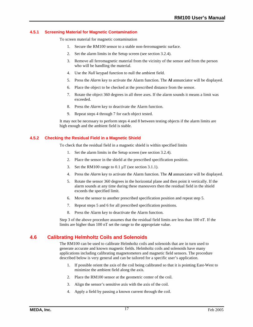
4.5.1 Screening Material for Magnetic Contamination To screen material for magnetic contamination
1. Secure the RM100 sensor to a stable non-ferromagnetic surface.
2. Set the alarm limits in the Setup screen (see section 3.2.4).
3. Remove all ferromagnetic material from the vicinity of the sensor and from the person who will be handling the material.
4. Use the Null keypad function to null the ambient field.
5. Press the Alarm key to activate the Alarm function. The Al annunciator will be displayed.
6. Place the object to be checked at the prescribed distance from the sensor.
7. Rotate the object 360 degrees in all three axes. If the alarm sounds it means a limit was exceeded.
8. Press the Alarm key to deactivate the Alarm function.
9. Repeat steps 4 through 7 for each object tested.
It may not be necessary to perform steps 4 and 8 between testing objects if the alarm limits are high enough and the ambient field is stable.
4.5.2 Checking the Residual Field in a Magnetic Shield To check that the residual field in a magnetic shield is within specified limits
1. Set the alarm limits in the Setup screen (see section 3.2.4).
2. Place the sensor in the shield at the prescribed specification position.
3. Set the RM100 range to 0.1 µT (see section 3.1.1).
4. Press the Alarm key to activate the Alarm function. The Al annunciator will be displayed.
5. Rotate the sensor 360 degrees in the horizontal plane and then point it vertically. If the alarm sounds at any time during these maneuvers then the residual field in the shield exceeds the specified limit.
6. Move the sensor to another prescribed specification position and repeat step 5.
7. Repeat steps 5 and 6 for all prescribed specification positions.
8. Press the Alarm key to deactivate the Alarm function.
Step 3 of the above procedure assumes that the residual field limits are less than 100 nT. If the limits are higher than 100 nT set the range to the appropriate value.
4.6 Calibrating Helmholtz Coils and Solenoids The RM100 can be used to calibrate Helmholtz coils and solenoids that are in turn used to generate accurate and known magnetic fields. Helmholtz coils and solenoids have many applications including calibrating magnetometers and magnetic field sensors. The procedure described below is very general and can be tailored for a specific user’s application.
1. If possible orient the axis of the coil being calibrated so that it is pointing East-West to minimize the ambient field along the axis.
2. Place the RM100 sensor at the geometric center of the coil.
3. Align the sensor’s sensitive axis with the axis of the coil.
4. Apply a field by passing a known current through the coil.
RM100 User’s Manual
Feb 2005 MEDA, Inc. 18
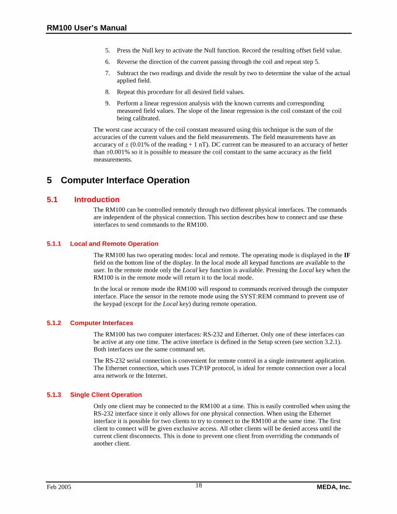
5. Press the Null key to activate the Null function. Record the resulting offset field value.
6. Reverse the direction of the current passing through the coil and repeat step 5.
7. Subtract the two readings and divide the result by two to determine the value of the actual applied field.
8. Repeat this procedure for all desired field values.
9. Perform a linear regression analysis with the known currents and corresponding measured field values. The slope of the linear regression is the coil constant of the coil being calibrated.
The worst case accuracy of the coil constant measured using this technique is the sum of the accuracies of the current values and the field measurements. The field measurements have an accuracy of ± (0.01% of the reading + 1 nT). DC current can be measured to an accuracy of better than ±0.001% so it is possible to measure the coil constant to the same accuracy as the field measurements.
5 Computer Interface Operation
5.1 Introduction The RM100 can be controlled remotely through two different physical interfaces. The commands are independent of the physical connection. This section describes how to connect and use these interfaces to send commands to the RM100.
5.1.1 Local and Remote Operation The RM100 has two operating modes: local and remote. The operating mode is displayed in the IF field on the bottom line of the display. In the local mode all keypad functions are available to the user. In the remote mode only the Local key function is available. Pressing the Local key when the RM100 is in the remote mode will return it to the local mode.
In the local or remote mode the RM100 will respond to commands received through the computer interface. Place the sensor in the remote mode using the SYST:REM command to prevent use of the keypad (except for the Local key) during remote operation.
5.1.2 Computer Interfaces The RM100 has two computer interfaces: RS-232 and Ethernet. Only one of these interfaces can be active at any one time. The active interface is defined in the Setup screen (see section 3.2.1). Both interfaces use the same command set.
The RS-232 serial connection is convenient for remote control in a single instrument application. The Ethernet connection, which uses TCP/IP protocol, is ideal for remote connection over a local area network or the Internet.
5.1.3 Single Client Operation Only one client may be connected to the RM100 at a time. This is easily controlled when using the RS-232 interface since it only allows for one physical connection. When using the Ethernet interface it is possible for two clients to try to connect to the RM100 at the same time. The first client to connect will be given exclusive access. All other clients will be denied access until the current client disconnects. This is done to prevent one client from overriding the commands of another client.
RM100 User’s Manual
MEDA, Inc. Feb 2005 19
5.2 Preparing for RS-232 Operation
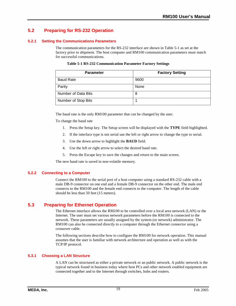
5.2.1 Setting the Communications Parameters The communication parameters for the RS-232 interface are shown in Table 5-1 as set at the factory prior to shipment. The host computer and RM100 communication parameters must match for successful communications.
Table 5-1 RS-232 Communication Parameter Factory Settings
Parameter Factory Setting
Baud Rate 9600
Parity None
Number of Data Bits 8
Number of Stop Bits 1
The baud rate is the only RM100 parameter that can be changed by the user.
To change the baud rate
1. Press the Setup key. The Setup screen will be displayed with the TYPE field highlighted.
2. If the interface type is not serial use the left or right arrow to change the type to serial.
3. Use the down arrow to highlight the BAUD field.
4. Use the left or right arrow to select the desired baud rate.
5. Press the Escape key to save the changes and return to the main screen.
The new baud rate is saved in non-volatile memory.
5.2.2 Connecting to a Computer Connect the RM100 to the serial port of a host computer using a standard RS-232 cable with a male DB-9 connector on one end and a female DB-9 connector on the other end. The male end connects to the RM100 and the female end connects to the computer. The length of the cable should be less than 50 feet (15 meters).
5.3 Preparing for Ethernet Operation The Ethernet interface allows the RM100 to be controlled over a local area network (LAN) or the Internet. The user must set various network parameters before the RM100 is connected to the network. These parameters are usually assigned by the system (or network) administrator. The RM100 can also be connected directly to a computer through the Ethernet connector using a crossover cable.
The following sections describe how to configure the RM100 for network operation. This manual assumes that the user is familiar with network architecture and operation as well as with the TCP/IP protocol.
5.3.1 Choosing a LAN Structure A LAN can be structured as either a private network or an public network. A public network is the typical network found in business today where host PCs and other network enabled equipment are connected together and to the Internet through switches, hubs and routers.
RM100 User’s Manual
Feb 2005 MEDA, Inc. 20
A private network is defined as a network consisting of host PCs and other network enabled equipment that is not connected to the public network or to the Internet. A private network can define its own IP addresses and other communication parameters without having them assigned by an internationally recognized authority.
5.3.2 Setting the Public Network Parameters The RM100 uses a static IP address to communicate over a network using the TCP/IP protocol. Before connecting the RM100 to the public network the user must obtain the following static IP parameters from the network administrator:
• Host IP address.
• Network mask.
• Gateway (router) IP address.
Once this information is gathered refer to section 3.2.3 for a description of how to enter this information into the RM100.
5.3.3 Setting Private Network Parameters The Internet Corporation for Assigned Names and Numbers (ICANN) assigned a set of numbers that can be used for private networks. If a device with one of these IP addresses is connected to the Internet it will not cause a disruption since routers automatically filter out these addresses. The following addresses are designated for private networks:
• 10.0.0.0 through 10.255.255.255 (a single Class A network)
• 172.16.0.0 through 172.31.255.255 (16 contiguous Class B networks)
• 192.168.0.0 through 192.168.255.255 (256 contiguous Class C networks)
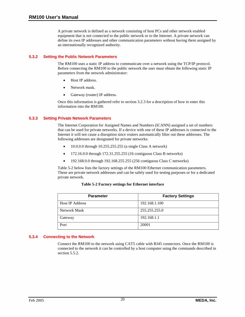
Table 5-2 below lists the factory settings of the RM100 Ethernet communication parameters. These are private network addresses and can be safely used for testing purposes or for a dedicated private network.
Table 5-2 Factory settings for Ethernet interface
Parameter Factory Settings
Host IP Address 192.168.1.100
Network Mask 255.255.255.0
Gateway 192.168.1.1
Port 20001
5.3.4 Connecting to the Network Connect the RM100 to the network using CAT5 cable with RJ45 connectors. Once the RM100 is connected to the network it can be controlled by a host computer using the commands described in section 5.5.2.
RM100 User’s Manual
MEDA, Inc. Feb 2005 21
5.4 Testing the Remote Interface After connecting the RM100 to the RS-232 or Ethernet interface, test the connection to see if it is operating properly. From the host computer run a terminal simulation program that can communicate with the specific interface being tested. For Microsoft Windows operating systems the program Hyper Terminal, which comes with the operating system, can be used to test both the RS-232 and the Ethernet connections. The following test procedures assume the terminal simulator is Hyper Terminal.
5.4.1 Testing the RS-232 Connection The following procedure assumes that a Hyper Terminal session has been initiated and the serial port parameters are identical to the RM100 settings.
1. Select Call->Disconnect from the Hyper Terminal menu to disconnect from the RS-232 interface.
2. Select File->Properties->Configure from the Hyper Terminal menu and verify that the communication parameters agree with the RM100 settings.
3. Click OK and select the Settings tab on the top of the dialog box.
4. Click on the ASCII Setup button.
5. Check the Send end lines with line feed and Echo typed characters locally boxes.
6. Click OK twice to return to the main screen.
7. Select Call from the Hyper Terminal Call main menu and then click on Call to connect to the RM100.
8. Send the following command: SYST:REM<CR> The <CR> represents a carriage return which is generated by pressing the Return key.
9. Hyper Terminal should echo the command. The IF field on the front panel of the RM100 should change from loc to rem.
10. Send the following command. *IDN?<CR>
11. The RM100 should respond with MEDA,RM100,nnnnnn,n.n nnnnnn is the RM100’s serial number; n.n is the firmware version.
The ERROR annunciator will be turned on if an error occurred. Use the SYST:ERR? command to retrieve the error message describing the cause of the error (section 3.10 explains how to retrieve error messages from the front panel).
5.4.2 Testing the Ethernet Connection The RM100 must be “reachable” from the network to which the host computer is connected. This means that the host and RM100 must have the same network address (masked portion of the IP address) or be connected through a router.
To test the network connection using a Microsoft Window operating system:
RM100 User’s Manual
Feb 2005 MEDA, Inc. 22
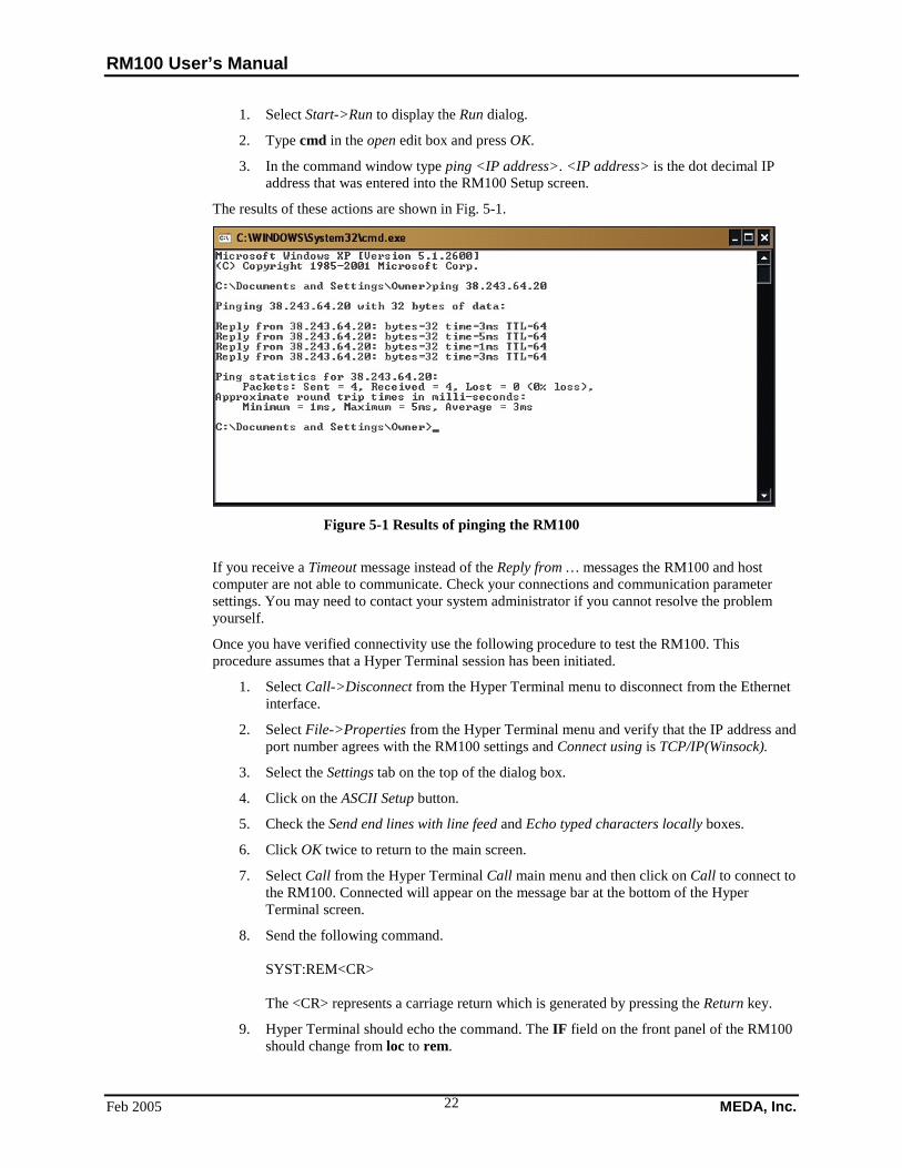
1. Select Start->Run to display the Run dialog.
2. Type cmd in the open edit box and press OK.
3. In the command window type ping <IP address>. <IP address> is the dot decimal IP address that was entered into the RM100 Setup screen.
The results of these actions are shown in Fig. 5-1.
Figure 5-1 Results of pinging the RM100
If you receive a Timeout message instead of the Reply from … messages the RM100 and host computer are not able to communicate. Check your connections and communication parameter settings. You may need to contact your system administrator if you cannot resolve the problem yourself.
Once you have verified connectivity use the following procedure to test the RM100. This procedure assumes that a Hyper Terminal session has been initiated.
1. Select Call->Disconnect from the Hyper Terminal menu to disconnect from the Ethernet interface.
2. Select File->Properties from the Hyper Terminal menu and verify that the IP address and port number agrees with the RM100 settings and Connect using is TCP/IP(Winsock).
3. Select the Settings tab on the top of the dialog box.
4. Click on the ASCII Setup button.
5. Check the Send end lines with line feed and Echo typed characters locally boxes.
6. Click OK twice to return to the main screen.
7. Select Call from the Hyper Terminal Call main menu and then click on Call to connect to the RM100. Connected will appear on the message bar at the bottom of the Hyper Terminal screen.
8. Send the following command. SYST:REM<CR> The <CR> represents a carriage return which is generated by pressing the Return key.
9. Hyper Terminal should echo the command. The IF field on the front panel of the RM100 should change from loc to rem.
RM100 User’s Manual
MEDA, Inc. Feb 2005 23
12. Send the following command. *IDN?<CR>
The RM100 should respond with MEDA,RM100,nnnnnn,n.n nnnnnn is the RM100’s serial number; n.n is the firmware version.
The ERROR annunciator will be turned on if an error occurred. Use the SYST:ERR? command to retrieve the error message describing the cause of the error (section 3.10 explains how to retrieve error messages from the front panel).
5.5 Command Processing The following sections describe how the RM100 processes commands received through the computer interface and what it sends back to the computer interface in response to the command. The RM100 uses version 1999.0 SCPI (Standard Commands for Programmable Instruments) syntax described in the SCPI Consortiums standards. These standards can be obtained from:
SCPI Consortium 2515 Camino del Rio South, Suite 340 San Diego, CA 92108
They can also be downloaded from their web site: http://www.scpiconsortium.org.
5.5.1 How SCPI Commands are Structured and Executed The SCPI language uses a “tree” structure similar to the file structure used in computer operating systems. There is a set of top level or “root” commands. Beneath each root level command there are associated sublevel commands and so on. The complete path (root->subroot>subsubroot etc) must be specified before it can be executed. An example command is shown below:
:SENSor:NULL:STATe ON<CR>
The capital letters are required. The lower case letters are optional. The command string is case insensitive. You can use either the abbreviated or the full command name but nothing else, otherwise you will generate an -113, “Undefined header” error.
In this example :SENSor is the root command; :NULL is a subcommand of SENSor and STATe is a subcommand of NULL. ON is a parameter of the STATe subcommand. The <CR> at the end of the line indicates to the RM100 that the command is complete and to process it. This command sets the state of the null condition of the RM100 to ON. This causes the RM100 to null the ambient field in the same way as if the user had pressed the Null key on the front panel.
The colon in the front of the first command indicates that it is a root command. If the root command is the first command in the string the colon is not needed.
5.5.2 Sending Multiple Commands in One Command String Multiple commands can be included in the command string. The SCPI language uses a semicolon to separate the commands. An example follows:
:SENS:NULL:STAT ON;:SENS:NULL:VALUE?;:READ?
This command string includes three commands separated by semicolons. The first command causes the RM100 to null the ambient field. The second command request that the value of the offset (nulling) field be returned to the computer. The third command requested that the value of the difference field (ambient field – offset field) be returned to the computer.
RM100 User’s Manual
Feb 2005 MEDA, Inc. 24
If an error occurs in executing the command the ERROR annunciator will turned on. The commands up to the point of an error are executed. Commands following an error are not executed. There are many possible sources of errors. The most common ones are syntax errors, missing parameters and parameter values that are out of bounds. Use the :SYST:ERR? Command to retrieve error messages.
In a command string that contains multiple commands, if the next command in the string is on the same level as the last substring the upper level portion of the path does not need to be included. The above command could have been entered as follows:
:SENS:NULL:STATE ON;VALUE?;:READ?
Since STATE and VALUE have the SENS:NULL path in common there is no need to repeat this path information in front of the VALUE? command.
The READ command needs a colon in front of it since it is a root command and is not in the same branch as the SENS commands.
White space (spaces and tabs) are allowed anywhere within the command string. A white space is required between a command and its associated parameters such as ON in the above example.
Commands that have a ? at the end return information to the computer.
5.5.3 How the Computer Receives Data Some commands, such as :READ?, return data. When a command returns data the data is followed by a <CR><LF> combination. For example the :READ? command would return
-42192<CR><LF>
where -42192 is the value of the field.
Some commands return multiple values. The :FETCH? command is an example. Each returned measurement point is separated by a comma. The last measurement point is followed by a <CR><LF> combination. This is illustrated in the following example:
Command -> :FET?<CR><LF>
Response -> -14365.2,-14366.0,-14370.3,-14371.5,-14360.4<CR><LF>
In this example five (5) measurement points were returned.
Another example is the :SYS:DATE? command.
Command -> :SYST:DATE?
Response -> 2004,7,22<CR><LF>
In this example 2004 is the year, 7 is the month and 22 is the day.
White space may precede each value in the returned string between the comma and the first significant digit.
5.5.4 How the RM100 Indicates Over Range of Invalid Data The data returned to the computer when the RM100 is in an over range (OVR) condition will be +9.9E37. An over range condition can also generate invalid statistical data. When a statistical value has invalid data associated with it the RM100 will return +9.9E37, which indicates the value is not-a-number (NAN).
Commands that can return this value include READ?, FET?, CALC:AVER:AVER?, CALC:AVER:MIN?, CALC:AVER:MAX?, CALC:AVER:PTP?, SAMP:AVER?, SAMP:MIN?, SAMP:MAX?, and SAMP:PTP?
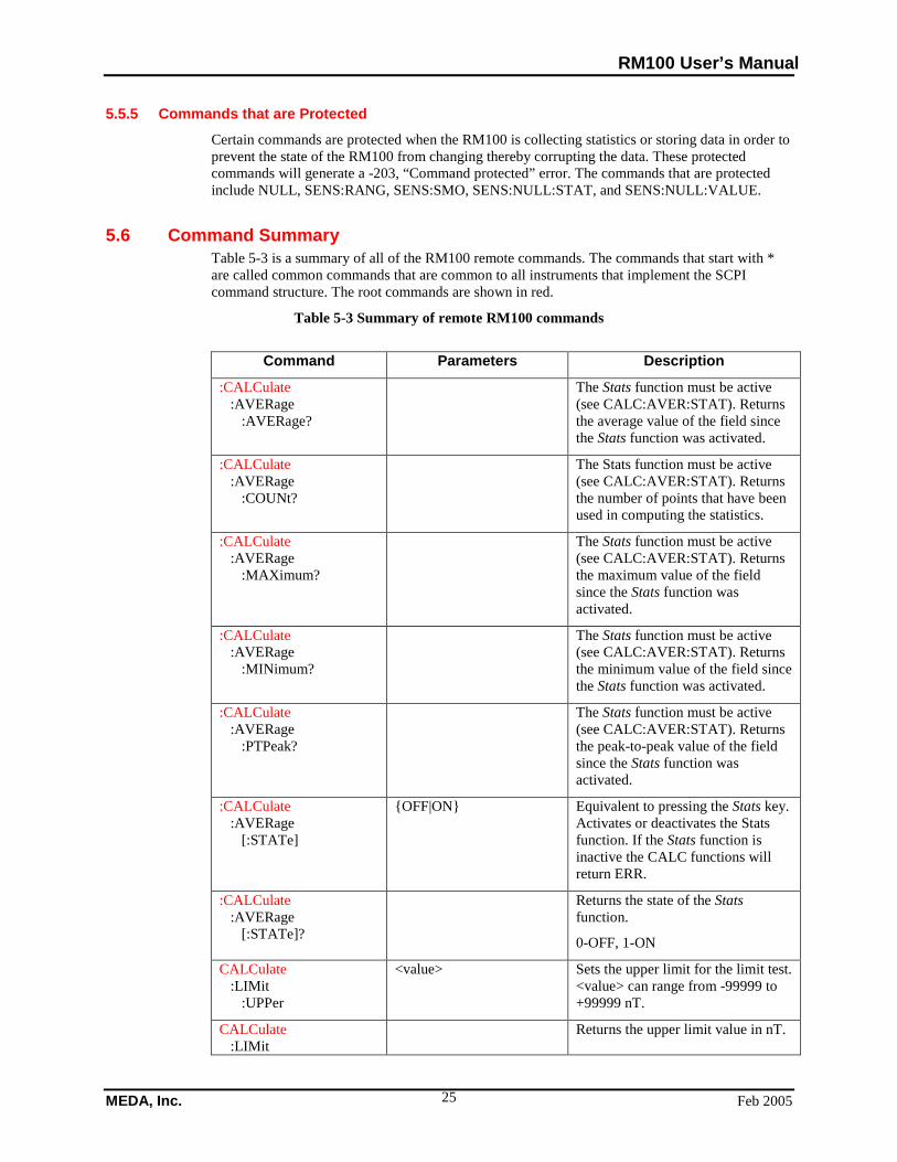
RM100 User’s Manual
MEDA, Inc. Feb 2005 25
5.5.5 Commands that are Protected Certain commands are protected when the RM100 is collecting statistics or storing data in order to prevent the state of the RM100 from changing thereby corrupting the data. These protected commands will generate a -203, “Command protected” error. The commands that are protected include NULL, SENS:RANG, SENS:SMO, SENS:NULL:STAT, and SENS:NULL:VALUE.
5.6 Command Summary Table 5-3 is a summary of all of the RM100 remote commands. The commands that start with * are called common commands that are common to all instruments that implement the SCPI command structure. The root commands are shown in red.
Table 5-3 Summary of remote RM100 commands
Command Parameters Description
:CALCulate :AVERage :AVERage?
The Stats function must be active (see CALC:AVER:STAT). Returns the average value of the field since the Stats function was activated.
:CALCulate :AVERage :COUNt?
The Stats function must be active (see CALC:AVER:STAT). Returns the number of points that have been used in computing the statistics.
:CALCulate :AVERage :MAXimum?
The Stats function must be active (see CALC:AVER:STAT). Returns the maximum value of the field since the Stats function was activated.
:CALCulate :AVERage :MINimum?
The Stats function must be active (see CALC:AVER:STAT). Returns the minimum value of the field since the Stats function was activated.
:CALCulate :AVERage :PTPeak?
The Stats function must be active (see CALC:AVER:STAT). Returns the peak-to-peak value of the field since the Stats function was activated.
:CALCulate :AVERage [:STATe]
{OFF|ON} Equivalent to pressing the Stats key. Activates or deactivates the Stats function. If the Stats function is inactive the CALC functions will return ERR.
:CALCulate :AVERage [:STATe]?
Returns the state of the Stats function.
0-OFF, 1-ON
CALCulate :LIMit :UPPer
<value> Sets the upper limit for the limit test. <value> can range from -99999 to +99999 nT.
CALCulate :LIMit
Returns the upper limit value in nT.
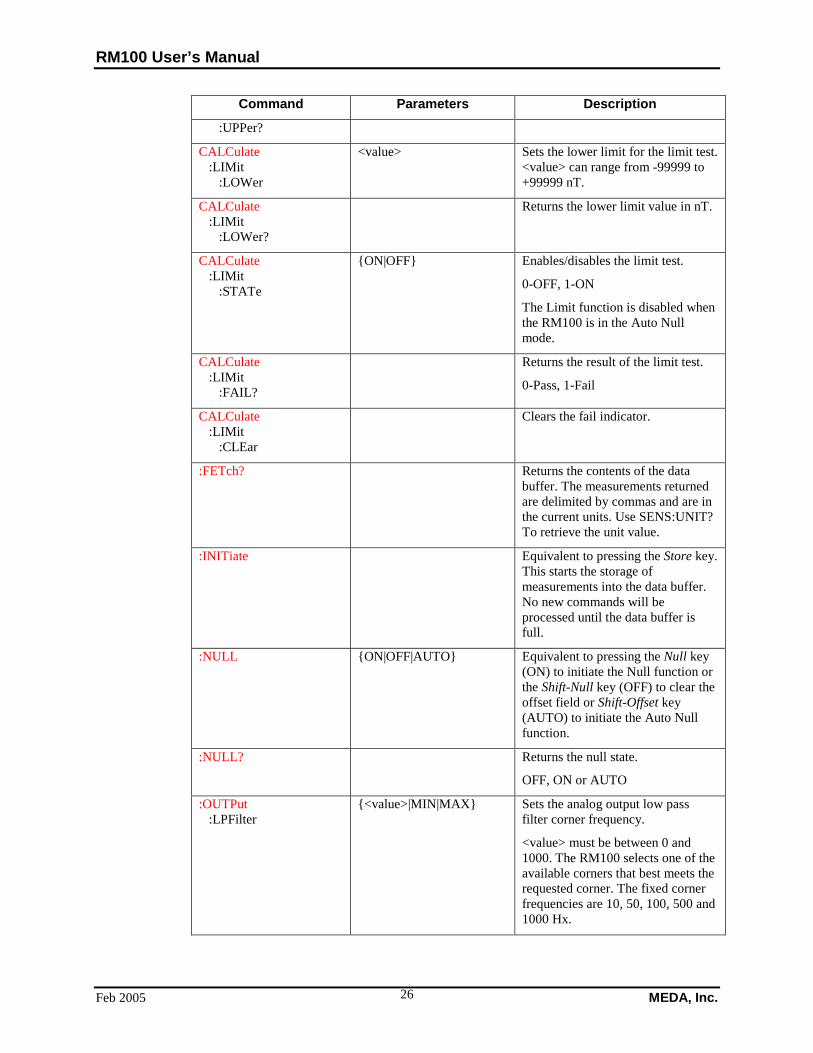
RM100 User’s Manual
Feb 2005 MEDA, Inc. 26
Command Parameters Description
:UPPer?
CALCulate :LIMit :LOWer
<value> Sets the lower limit for the limit test. <value> can range from -99999 to +99999 nT.
CALCulate :LIMit :LOWer?
Returns the lower limit value in nT.
CALCulate :LIMit :STATe
{ON|OFF} Enables/disables the limit test.
0-OFF, 1-ON
The Limit function is disabled when the RM100 is in the Auto Null mode.
CALCulate :LIMit :FAIL?
Returns the result of the limit test.
0-Pass, 1-Fail
CALCulate :LIMit :CLEar
Clears the fail indicator.
:FETch? Returns the contents of the data buffer. The measurements returned are delimited by commas and are in the current units. Use SENS:UNIT? To retrieve the unit value.
:INITiate Equivalent to pressing the Store key. This starts the storage of measurements into the data buffer. No new commands will be processed until the data buffer is full.
:NULL {ON|OFF|AUTO} Equivalent to pressing the Null key (ON) to initiate the Null function or the Shift-Null key (OFF) to clear the offset field or Shift-Offset key (AUTO) to initiate the Auto Null function.
:NULL? Returns the null state.
OFF, ON or AUTO
:OUTPut :LPFilter
{<value>|MIN|MAX} Sets the analog output low pass filter corner frequency.
<value> must be between 0 and 1000. The RM100 selects one of the available corners that best meets the requested corner. The fixed corner frequencies are 10, 50, 100, 500 and 1000 Hx.
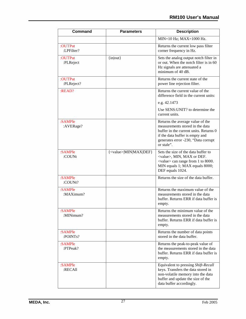
RM100 User’s Manual
MEDA, Inc. Feb 2005 27
Command Parameters Description
MIN=10 Hz; MAX=1000 Hz.
:OUTPut :LPFilter?
Returns the current low pass filter corner frequency in Hz.
:OUTPut :PLReject
{in|out} Sets the analog output notch filter in or out. When the notch filter is in 60 Hz signals are attenuated a minimum of 40 dB.
:OUTPut :PLReject?
Returns the current state of the power line rejection filter.
:READ? Returns the current value of the difference field in the current units:
e.g. 42.1473
Use SENS:UNIT? to determine the current units.
:SAMPle :AVERage?
Returns the average value of the measurements stored in the data buffer in the current units. Returns 0 if the data buffer is empty and generates error -230, “Data corrupt or stale”.
:SAMPle :COUNt
{<value>|MIN|MAX|DEF} Sets the size of the data buffer to <value>, MIN, MAX or DEF. <value> can range from 1 to 8000. MIN equals 1; MAX equals 8000; DEF equals 1024.
:SAMPle :COUNt?
Returns the size of the data buffer.
:SAMPle :MAXimum?
Returns the maximum value of the measurements stored in the data buffer. Returns ERR if data buffer is empty.
:SAMPle :MINimum?
Returns the minimum value of the measurements stored in the data buffer. Returns ERR if data buffer is empty.
:SAMPle :POINTs?
Returns the number of data points stored in the data buffer.
:SAMPle :PTPeak?
Returns the peak-to-peak value of the measurements stored in the data buffer. Returns ERR if data buffer is empty.
:SAMPle :RECAll
Equivalent to pressing Shift-Recall keys. Transfers the data stored in non-volatile memory into the data buffer and update the size of the data buffer accordingly.
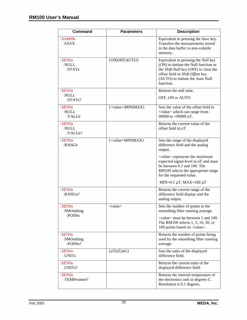
RM100 User’s Manual
Feb 2005 MEDA, Inc. 28
Command Parameters Description
:SAMPle :SAVE
Equivalent to pressing the Save key. Transfers the measurements stored in the data buffer to non-volatile memory.
:SENSe :NULL :STATe
{ON|OFF|AUTO} Equivalent to pressing the Null key (ON) to initiate the Null function or the Shift-Null key (OFF) to clear the offset field or Shift-Offset key (AUTO) to initiate the Auto Null function.
:SENSe :NULL :STATe?
Returns the null state.
OFF, ON or AUTO
:SENSe :NULL :VALUe
{<value>|MIN|MAX} Sets the value of the offset field to <value> which can range from -99999 to +99999 nT.
:SENSe :NULL :VALUe?
Returns the current value of the offset field in nT.
:SENSe :RANGe
{<value>MIN|MAX} Sets the range of the displayed difference field and the analog output.
<value> represents the maximum expected signal level in uT and must be between 0.1 and 100. The RM100 selects the appropriate range for the requested value.
MIN=0.1 µT; MAX=100 µT
:SENSe :RANGe?
Returns the current range of the difference field display and the analog output.
:SENSe :SMOothing :POINts
<value> Sets the number of points in the smoothing filter running average.
<value> must be between 1 and 100. The RM100 selects 1, 3, 10, 50, or 100 points based on <value>.
:SENSe :SMOothing :POINts?
Returns the number of points being used by the smoothing filter running average.
:SENSe :UNITs
{uT|nT|mG} Sets the units of the displayed difference field.
:SENSe :UNITs?
Returns the current units of the displayed difference field.
:SENSe :TEMPerature?
Returns the internal temperature of the electronics unit in degrees C. Resolution is 0.1 degrees.
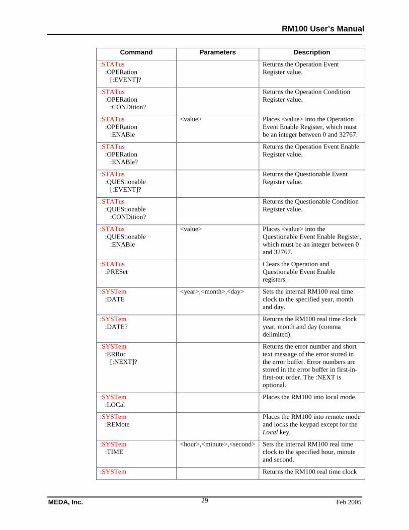
RM100 User’s Manual
MEDA, Inc. Feb 2005 29
Command Parameters Description
:STATus :OPERation [:EVENT]?
Returns the Operation Event Register value.
:STATus :OPERation :CONDition?
Returns the Operation Condition Register value.
:STATus :OPERation :ENABle
<value> Places <value> into the Operation Event Enable Register, which must be an integer between 0 and 32767.
:STATus :OPERation :ENABle?
Returns the Operation Event Enable Register value.
:STATus :QUEStionable [:EVENT]?
Returns the Questionable Event Register value.
:STATus :QUEStionable :CONDition?
Returns the Questionable Condition Register value.
:STATus :QUEStionable :ENABle
<value> Places <value> into the Questionable Event Enable Register, which must be an integer between 0 and 32767.
:STATus :PRESet
Clears the Operation and Questionable Event Enable registers.
:SYSTem :DATE
<year>,<month>,<day> Sets the internal RM100 real time clock to the specified year, month and day.
:SYSTem :DATE?
Returns the RM100 real time clock year, month and day (comma delimited).
:SYSTem :ERRor [:NEXT]?
Returns the error number and short text message of the error stored in the error buffer. Error numbers are stored in the error buffer in first-in-first-out order. The :NEXT is optional.
:SYSTem :LOCal
Places the RM100 into local mode.
:SYSTem :REMote
Places the RM100 into remote mode and locks the keypad except for the Local key.
:SYSTem :TIME
<hour>,<minute>,<second> Sets the internal RM100 real time clock to the specified hour, minute and second.
:SYSTem Returns the RM100 real time clock
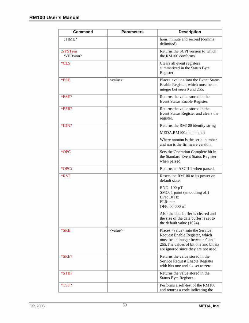
RM100 User’s Manual
Feb 2005 MEDA, Inc. 30
Command Parameters Description
:TIME? hour, minute and second (comma delimited).
:SYSTem :VERsion?
Returns the SCPI version to which the RM100 conforms.
*CLS Clears all event registers summarized in the Status Byte Register.
*ESE <value> Places <value> into the Event Status Enable Register, which must be an integer between 0 and 255.
*ESE? Returns the value stored in the Event Status Enable Register.
*ESR? Returns the value stored in the Event Status Register and clears the register.
*IDN? Returns the RM100 identity string
MEDA,RM100,nnnnnn,n.n
Where nnnnnn is the serial number and n.n is the firmware version.
*OPC Sets the Operation Complete bit in the Standard Event Status Register when parsed.
*OPC? Returns an ASCII 1 when parsed.
*RST Resets the RM100 to its power on default state:
RNG: 100 µT SMO: 1 point (smoothing off) LPF: 10 Hz PLR: out OFF: 00,000 nT
Also the data buffer is cleared and the size of the data buffer is set to the default value (1024).
*SRE <value> Places <value> into the Service Request Enable Register, which must be an integer between 0 and 255.The values of bit one and bit six are ignored since they are not used.
*SRE? Returns the value stored in the Service Request Enable Register with bits one and six set to zero.
*STB? Returns the value stored in the Status Byte Register.
*TST? Performs a self-test of the RM100 and returns a code indicating the
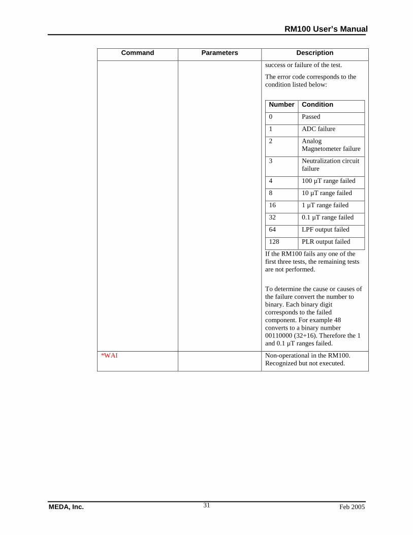
RM100 User’s Manual
MEDA, Inc. Feb 2005 31
Command Parameters Description
success or failure of the test.
The error code corresponds to the condition listed below:
Number Condition
0 Passed
1 ADC failure
2 Analog Magnetometer failure
3 Neutralization circuit failure
4 100 µT range failed
8 10 µT range failed
16 1 µT range failed
32 0.1 µT range failed
64 LPF output failed
128 PLR output failed
If the RM100 fails any one of the first three tests, the remaining tests are not performed.
To determine the cause or causes of the failure convert the number to binary. Each binary digit corresponds to the failed component. For example 48 converts to a binary number 00110000 (32+16). Therefore the 1 and 0.1 µT ranges failed.
*WAI Non-operational in the RM100. Recognized but not executed.
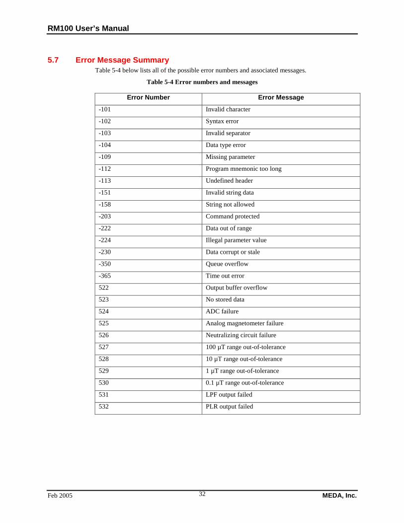
RM100 User’s Manual
Feb 2005 MEDA, Inc. 32
5.7 Error Message Summary Table 5-4 below lists all of the possible error numbers and associated messages.
Table 5-4 Error numbers and messages
Error Number Error Message
-101 Invalid character
-102 Syntax error
-103 Invalid separator
-104 Data type error
-109 Missing parameter
-112 Program mnemonic too long
-113 Undefined header
-151 Invalid string data
-158 String not allowed
-203 Command protected
-222 Data out of range
-224 Illegal parameter value
-230 Data corrupt or stale
-350 Queue overflow
-365 Time out error
522 Output buffer overflow
523 No stored data
524 ADC failure
525 Analog magnetometer failure
526 Neutralizing circuit failure
527 100 µT range out-of-tolerance
528 10 µT range out-of-tolerance
529 1 µT range out-of-tolerance
530 0.1 µT range out-of-tolerance
531 LPF output failed
532 PLR output failed
RM100 User’s Manual
MEDA, Inc. Feb 2005 33
5.8 Status Structure The RM100 conforms to the SCPI status register structure. There are three event registers with associated event enable registers that feed a Status Byte register that summarizes the status of the RM100. This structure is illustrated in Fig. 5-2.
5.8.1 Status Byte Register The bits in the Status Byte Register (SBR) indicate the state of the event registers, the Output Queue and the Error Queue. The SRQ bit depends on the state of the SRB and the Service Request Enable (SRE) register. The SRQ bit is controlled by the SRE register. The SBR bits are logically ANDed (&) with the corresponding bits of the SRE register and the results ORed to determine the state of the SRQ bit. The bits in the SBR do not latch. Their state (0 or 1) indicates the state of their associated event register or queue.
Use the *STB? query command to read the condition of the SBR. Then read the specific event register using the appropriate query command to determine the cause of an event. The query commands are listed in Table 5-3.
5.8.2 Questionable Event Register The Questionable Event Register (QER) indicates events that compromise the measurements being made. Only two events are indicated:
• Bit 8 - Calibration Error. Sset if an error occurred during the self-test that occurs when the RM100 is first turned on or in response to the *TST command.
• Bit 9 - Over Range. Set whenever the measurement results in an over range error.
The bits in the QER are latched until reset by reading the register or issuing a *CLS command. Use the :STAT:QUES? command to read the contents of the QER.
The state of the QER is reported to the SBR based on the contents of the Questionable Event Enable (QEE) register. The QER bits are ANDed with the corresponding QEE register bits and the results ORed to determine the state of the QSB bit in the SBR. Enable the reporting of a QER event by setting the corresponding bit in the QEE to 1. Use the :STAT:QUES:ENAB command to set the bits in the QEE (see Table 5-1).
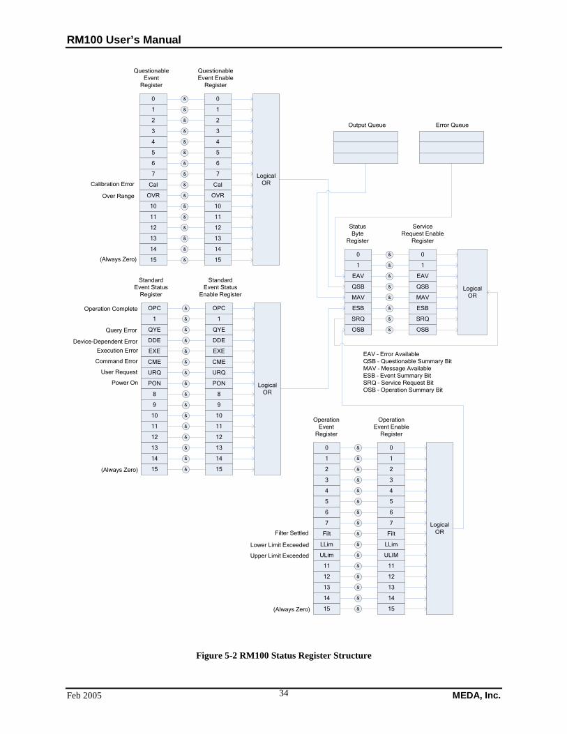
RM100 User’s Manual
Feb 2005 MEDA, Inc. 34
0
1
2
3
4
5
6
7
Cal
OVR
10
11
12
13
14
15
0
1
2
3
4
5
6
7
Cal
OVR
10
11
12
13
14
15
&
&
&
&
&
&
&
&
&
&
&
&
&
&
&
&
LogicalOR
OPC
1
QYE
DDE
EXE
CME
URQ
PON
8
9
10
11
12
13
14
15
OPC
1
QYE
DDE
EXE
CME
URQ
PON
8
9
10
11
12
13
14
15
&
&
&
&
&
&
&
&
&
&
&
&
&
&
&
&
LogicalOR
0
1
2
3
4
5
6
7
Filt
LLim
ULim
11
12
13
14
15
0
1
2
3
4
5
6
7
Filt
LLim
ULIM
11
12
13
14
15
&
&
&
&
&
&
&
&
&
&
&
&
&
&
&
&
LogicalOR
(Always Zero)
Over Range
Calibration Error
Operation Complete
Query Error
Device-Dependent ErrorExecution Error
Command Error
User Request
Power On
(Always Zero)
(Always Zero)
Filter Settled
Lower Limit Exceeded
Upper Limit Exceeded
QuestionableEvent
Register
QuestionableEvent Enable
Register
StandardEvent Status
Register
StandardEvent Status
Enable Register
OperationEvent
Register
OperationEvent Enable
Register
0
1
EAV
QSB
MAV
ESB
SRQ
OSB
0
1
EAV
QSB
MAV
ESB
SRQ
OSB
&
&
&
&
&
&
&
&
LogicalOR
StatusByte
Register
ServiceRequest Enable
Register
Output Queue Error Queue
EAV – Error AvailableQSB – Questionable Summary BitMAV – Message AvailableESB – Event Summary BitSRQ – Service Request BitOSB – Operation Summary Bit
Figure 5-2 RM100 Status Register Structure
RM100 User’s Manual
MEDA, Inc. Feb 2005 35
5.8.3 Standard Event Status Register The Standard Event Status (ESR) register bits correspond to the following events:
• Bit 0 – Operation Complete (OPC). Indicates that all pending operations are complete. This bit is set only in response to the *OPC command.
• Bit 1 – Not used.
• Bit 2 – Query Error. Not used.
• Bit 3 – Device Dependent Error. Not used.
• Bit 4 – Execution error. Set if there was an error in executing a command.
• Bit 5 – Command Error. Set when there was an error in the command sent to the RM100.
• Bit 6 – User request. Not used.
• Bit 7 – Power On (PON). This bit indicates that the RM100 was turned off and then back on since the last time this register was read.
The bits in the ESR are latched until reset by reading the register or issuing a *CLS command. Use the *ESR? command to read the contents of the ESR.
The state of the ESR is reported to the SBR based on the contents of the Standard Event Status Enable (ESE) register. The ESR bits are ANDed with the corresponding ESE register bits and the results ORed to determine the state of the ESB bit in the SBR. Enable the reporting of an ESR event by setting the corresponding bit in the ESE to 1. Use the *ESE command to set the bits in the ESE register (see Table 5-1).
5.8.4 Operation Event Register The Operation Event Status (OES) register bits correspond to the following events:
• Bit 0 through Bit 7 – Unused.
• Bit 8 – Filter Settled. Indicates that the running average filter has settled.
• Bit 9 – Lower Limit Failed. Set when the lower limit test fails.
• Bit 10 – Upper Limit Failed. Set when the lower limit test fails.
• Bit 11 through Bit 15 – Unused.
The bits in the OES register are latched until reset by reading the register or issuing a *CLS command. Use the :STAT:OPER? command to read the contents of the OES register.
The state of the OES register is reported to the SBR based on the contents of the Operation Event Status Enable (OESE) register. The OES register bits are ANDed with the corresponding OESE register bits and the results ORed to determine the state of the OSB bit in the SBR. Enable the reporting of an ESR event by setting the corresponding bit in the ESE to 1. Use the :STAT:OPER:ENAB command to set the bits in the OESE register (see Table 5-1).
5.8.5 Clearing the Event and Event Enable Registers The event and event enable registers are cleared when the RM100 is first turned on. These registers can be cleared programmatically using the following commands:
• *CLS – Resets all bits in the Standard, Operation and Questionable Event Registers.
• :STAT:PRES – Resets all bits in the Operation and Questionable Event Enable Registers.
• *ESE 0 – Resets the Event Status Enable Register.
RM100 User’s Manual
Feb 2005 MEDA, Inc. 36
6 Theory of Operation
6.1 Introduction This section provides a description of how the RM100 works. The first subsection gives an overview of the RM100. Subsequent sections go into greater detail. The objective is to provide sufficient detail for you to understand how best to use the RM100 in your applications.
6.2 Overview Figure 6-1 is a block diagram of the RM100.
The RM100 is divided into two major components: the Sensor Unit (SU) and the Electronics Unit (EU). The SU contains the fluxgate sensor that includes three windings: the excitation winding, the signal winding and the neutralization winding. The EU contains the circuitry needed to excite the sensor, process the sensor signal, display the results to the user and respond to user front panel and remote command.
6.2.1 Embedded Microprocessor An RCM2200 microprocessor controls the RM100 functions. It responds to front panel keypad commands and commands received through either the RS-232 serial interface or the Ethernet interface. The RM100 firmware is stored in a 512 K flash memory. The flash memory is also used to store buffer data in response to the Store command. A 512K RAM is used to store temporary data.
6.2.2 User Interface The front 4 x 4 membrane switch matrix key pad provides a front panel user interface. The columns of the matrix are periodically activated and the rows read by the microprocessor. The microprocessor interprets these switch closures as user commands.
A 256 x 64 dot vacuum fluorescent graphics display provides the user with measurement results, plots and other data.
6.2.3 Analog Data Filtering and Conversion A 22-bit analog-to-digital converter (ADC) converts the analog voltage from the sensor signal conditioner into a digital form that is processed by the microprocessor. The signal conditioner analog output is also fed to the input of a programmable low pass filter. The low pass filter output is available through a connector on the RM100 back panel. The user can also insert a power line rejection filter between the signal conditioner analog output and the low pass filter to reduce unwanted power line signals.
An 18-bit digital-to-analog converter (DAC) generates the voltages that are converted by the neutralization circuit into a current in the neutralization winding to create the offset field.
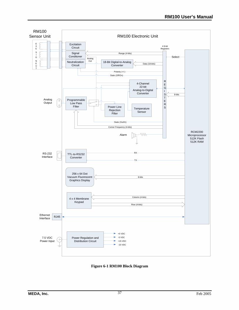
RM100 User’s Manual
MEDA, Inc. Feb 2005 37
ExcitationCircuit
SignalConditoner
NeutralizationCircuit
4-Channel22-bit
Analog-to-DigitalConverter
ProgrammableLow Pass
Filter Power Line Rejection
Filter
TemperatureSensor
EXE
SIG
NEUT
18-Bit Digital-to-Analog Converter
TTL-to-RS232 Converter
State (Out/In)
Alarm
REGISTERS
Polarity (+/-)
State (Off/On)
Analog Out
Data (18-bits)
Corner Frequency (4-bits)
Range (4-bits)
256 x 64 Dot Vacuum Fluorescent
Graphics Display
4 x 4 Membrane Keypad
RCM2200 Microprocessor
512K Flash512K RAM
8-bits
Select
4 8-bit Registers
8-bits
RX
TX
Column (4-bits)
Row (4-bits)
Power Regulation and Distribution Circuit
+5 VDC
-5 VDC
+15 VDC
-15 VDC
RM100 Electronic UnitRM100
Sensor Unit
Analog Output
RS-232 Interface
7.5 VDC Power Input
RJ45Ethernet Interface
Figure 6-1 RM100 Block Diagram
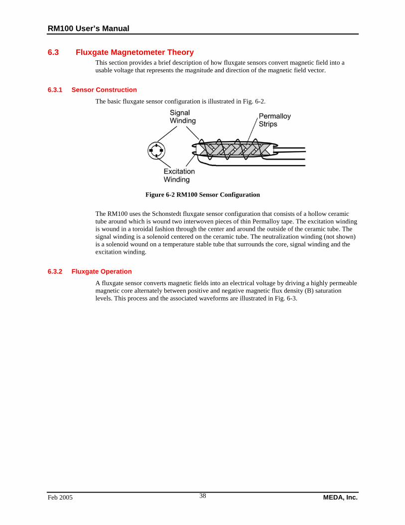
RM100 User’s Manual
Feb 2005 MEDA, Inc. 38
6.3 Fluxgate Magnetometer Theory This section provides a brief description of how fluxgate sensors convert magnetic field into a usable voltage that represents the magnitude and direction of the magnetic field vector.
6.3.1 Sensor Construction The basic fluxgate sensor configuration is illustrated in Fig. 6-2.
Figure 6-2 RM100 Sensor Configuration
The RM100 uses the Schonstedt fluxgate sensor configuration that consists of a hollow ceramic tube around which is wound two interwoven pieces of thin Permalloy tape. The excitation winding is wound in a toroidal fashion through the center and around the outside of the ceramic tube. The signal winding is a solenoid centered on the ceramic tube. The neutralization winding (not shown) is a solenoid wound on a temperature stable tube that surrounds the core, signal winding and the excitation winding.
6.3.2 Fluxgate Operation A fluxgate sensor converts magnetic fields into an electrical voltage by driving a highly permeable magnetic core alternately between positive and negative magnetic flux density (B) saturation levels. This process and the associated waveforms are illustrated in Fig. 6-3.
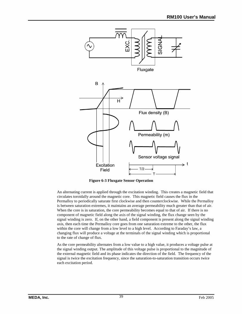
RM100 User’s Manual
MEDA, Inc. Feb 2005 39
Figure 6-3 Fluxgate Sensor Operation
An alternating current is applied through the excitation winding. This creates a magnetic field that circulates toroidally around the magnetic core. This magnetic field causes the flux in the Permalloy to periodically saturate first clockwise and then counterclockwise. While the Permalloy is between saturation extremes, it maintains an average permeability much greater than that of air. When the core is in saturation, the core permeability becomes equal to that of air. If there is no component of magnetic field along the axis of the signal winding, the flux change seen by the signal winding is zero. If, on the other hand, a field component is present along the signal winding axis, then each time the Permalloy core goes from one saturation extreme to the other, the flux within the core will change from a low level to a high level. According to Faraday’s law, a changing flux will produce a voltage at the terminals of the signal winding which is proportional to the rate of change of flux.
As the core permeability alternates from a low value to a high value, it produces a voltage pulse at the signal winding output. The amplitude of this voltage pulse is proportional to the magnitude of the external magnetic field and its phase indicates the direction of the field. The frequency of the signal is twice the excitation frequency, since the saturation-to-saturation transition occurs twice each excitation period.
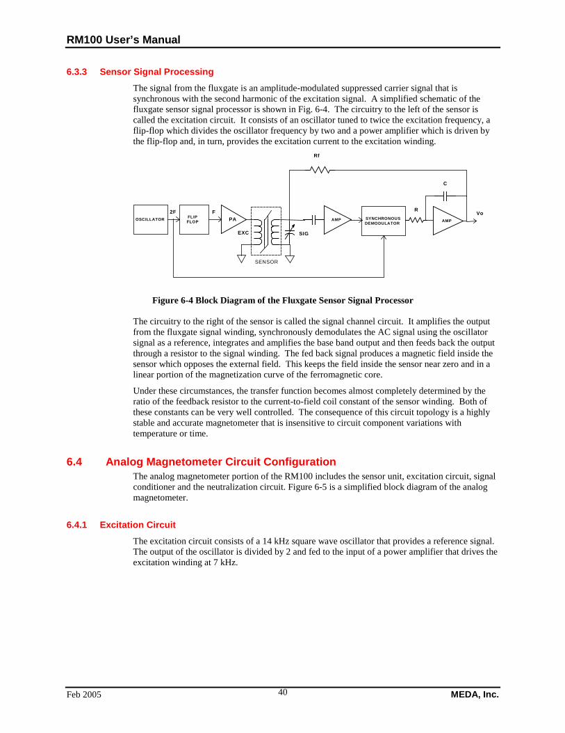
RM100 User’s Manual
Feb 2005 MEDA, Inc. 40
6.3.3 Sensor Signal Processing The signal from the fluxgate is an amplitude-modulated suppressed carrier signal that is synchronous with the second harmonic of the excitation signal. A simplified schematic of the fluxgate sensor signal processor is shown in Fig. 6-4. The circuitry to the left of the sensor is called the excitation circuit. It consists of an oscillator tuned to twice the excitation frequency, a flip-flop which divides the oscillator frequency by two and a power amplifier which is driven by the flip-flop and, in turn, provides the excitation current to the excitation winding.
OSCILLATOR FLIP FLOP PA AMP AMP SYNCHRONOUS
DEMODULATOR
Rf
F
C
R
EXC SIG
2F
SENSOR
Vo
Figure 6-4 Block Diagram of the Fluxgate Sensor Signal Processor
The circuitry to the right of the sensor is called the signal channel circuit. It amplifies the output from the fluxgate signal winding, synchronously demodulates the AC signal using the oscillator signal as a reference, integrates and amplifies the base band output and then feeds back the output through a resistor to the signal winding. The fed back signal produces a magnetic field inside the sensor which opposes the external field. This keeps the field inside the sensor near zero and in a linear portion of the magnetization curve of the ferromagnetic core.
Under these circumstances, the transfer function becomes almost completely determined by the ratio of the feedback resistor to the current-to-field coil constant of the sensor winding. Both of these constants can be very well controlled. The consequence of this circuit topology is a highly stable and accurate magnetometer that is insensitive to circuit component variations with temperature or time.
6.4 Analog Magnetometer Circuit Configuration The analog magnetometer portion of the RM100 includes the sensor unit, excitation circuit, signal conditioner and the neutralization circuit. Figure 6-5 is a simplified block diagram of the analog magnetometer.
6.4.1 Excitation Circuit The excitation circuit consists of a 14 kHz square wave oscillator that provides a reference signal. The output of the oscillator is divided by 2 and fed to the input of a power amplifier that drives the excitation winding at 7 kHz.
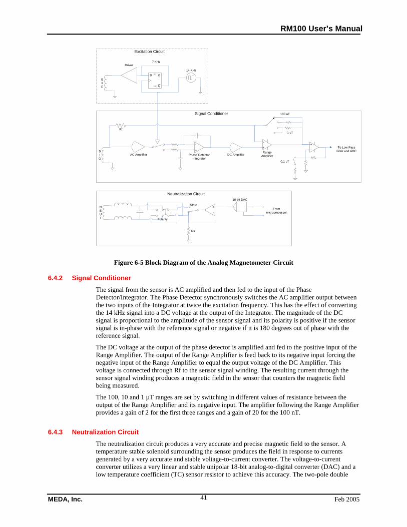
RM100 User’s Manual
MEDA, Inc. Feb 2005 41
EXE
SIG
NEUT
Driver
Q
QSET
CLR
D14 KHz
AC Amplifier Phase DetectorIntegrator
DC AmplifierRange
Amplifier
Rf
+
-+
-
-+
7 KHz
100 uT
1 uT
0.1 uT
To Low Pass Filter and ADC
Polarity
State
Rs
18-bit DAC
From microprocessor
+
-
Excitation Circuit
Signal Conditioner
Neutralization Circuit
Figure 6-5 Block Diagram of the Analog Magnetometer Circuit
6.4.2 Signal Conditioner The signal from the sensor is AC amplified and then fed to the input of the Phase Detector/Integrator. The Phase Detector synchronously switches the AC amplifier output between the two inputs of the Integrator at twice the excitation frequency. This has the effect of converting the 14 kHz signal into a DC voltage at the output of the Integrator. The magnitude of the DC signal is proportional to the amplitude of the sensor signal and its polarity is positive if the sensor signal is in-phase with the reference signal or negative if it is 180 degrees out of phase with the reference signal.
The DC voltage at the output of the phase detector is amplified and fed to the positive input of the Range Amplifier. The output of the Range Amplifier is feed back to its negative input forcing the negative input of the Range Amplifier to equal the output voltage of the DC Amplifier. This voltage is connected through Rf to the sensor signal winding. The resulting current through the sensor signal winding produces a magnetic field in the sensor that counters the magnetic field being measured.
The 100, 10 and 1 µT ranges are set by switching in different values of resistance between the output of the Range Amplifier and its negative input. The amplifier following the Range Amplifier provides a gain of 2 for the first three ranges and a gain of 20 for the 100 nT.
6.4.3 Neutralization Circuit The neutralization circuit produces a very accurate and precise magnetic field to the sensor. A temperature stable solenoid surrounding the sensor produces the field in response to currents generated by a very accurate and stable voltage-to-current converter. The voltage-to-current converter utilizes a very linear and stable unipolar 18-bit analog-to-digital converter (DAC) and a low temperature coefficient (TC) sensor resistor to achieve this accuracy. The two-pole double
RM100 User’s Manual
Feb 2005 MEDA, Inc. 42
throw switch controls the polarity of the field and the single-pole double throw switch turns the field off or on.
6.5 Analog Output Filtering The RM100 provides a filtered analog output that can be used to record magnetic field data. The output of the analog magnetometer connects to the input of the power line rejection filter and one position of a single-pole double throw switch. The power line rejection filter output connects to the other position of the switch. The pole of the switch connects to the input of a programmable 4-pole Butterworth low pass filter. The output of the low pass filter goes to a connector on the back panel of the RM100.
The low pass filter provides 24 dB per octave attenuation of frequencies beyond the -3 dB point. This filter essentially eliminates any ripple signals at the sensor excitation frequency and its harmonics.
When connected in the filter chain the power line rejection or notch filter provides at least 40 dB of attenuation of magnetic fields produced by power line current flow. The attenuation is at the fundamental frequency. The standard rejection frequency is 60 Hz (50 Hz is optional).
7 Maintenance The RM100 requires very little maintenance. There are no user adjustments. When the RM100 is turned on it performs a self-test to determine the health of the instrument. This self test can also be initiated remotely through the RS-232 or Ethernet connection using the *TST command. The RM100 should be in an area that is magnetically static during the test to prevent false error indications. In the event of a failure the instrument should be returned to MEDA for diagnostics and repair with a list of all error codes that were returned by the RM100 after the self-test.
7.1 Probe Precautions The health of the probe is very important for the reliable and accurate performance of the RM100. Do not expose the probe to fields greater than 500 µT (5 Gauss). The sensor could be magnetized causing a shift in zero field readings that will affect instrument accuracy.
The internal structure of the probe is fairly rugged but it does contain some structure that can be damaged by physical abuse. This damage can affect sensor alignment and neutralization field performance.
The probe is not waterproof and should not be place in water. The probe should be protected from moisture penetration if measurements are to be made in inclement weather.
7.2 Fuse Replacement The RM100 has one fuse that is accessible from the rear panel. If the fuse needs to be replaced press the fuse holder forward while turning clockwise to remove the holder. Remove the old fuse and replace it with a Littlefuse 312003 3A fuse or equivalent. Reinsert the fuse holder into the fuse case and turn counterclockwise while pressing the folder forward until it locks in place.
7.3 Calibration Cycle The RM100 should remain with specifications for at least one year. MEDA recommends that the instrument be calibrated annually. The RM100 must be returned to MEDA for calibration. The special equipment required to calibrate the RM100 is normally not available from a standard calibration laboratory.

RM100 User’s Manual
MEDA, Inc. Feb 2005 43
7.4 Firmware Update The RM100 firmware controls the operation of the magnetometer. It is stored in EEPROM on a microprocessor board inside the RM100. The firmware can be updated through the Ethernet connection. This section describes how to perform this task.
The firmware update will be provided in the form of a file named rm100a.bin. This file may be supplied on a disc, sent to you by email or downloaded from our ftp site. Whatever way it is obtained it should be placed in the directory from which you execute your local ftp client. You will need the IP address of the RM100 that you are updating. This can be obtained from the RM100 Setup Screen.
To update the firmware:
1. With the RM100 powered off connect the RM100 Ethernet connector to the local network or directly to the computer being used for the update (direct connection requires a crossover cable).
2. Start the ftp client on the computer where the firmware update file resides. On a Microsoft Windows operating system this can be done by opening a command window and typing ftp at the prompt. The prompt will change to ftp>.
3. Turn the RM100 power on. The front panel screen on the RM100 will display the following message: FTP server active for firmware update—hit key to continue.
4. On the PC following the ftp> prompt type open <rm100IPaddress>. Do not type in the brackets, just the RM100 IP address. The IP address should be in dot decimal format (e.g., 192.168.0.2).
5. The RM100 ftp server will respond with the following: Connected to <rm100IPaddress> 220 Hello! Welcome to MEDA RM100 Loader FTP! User (<rm100IPaddress>:(none)):
6. Type meda followed by the enter key. The server will respond with 331 Password required Password:
7. After the colon type rm100 followed by the enter key. The typing will not be echoed.
8. The server will respond with: 230 User logged in. ftp>
9. Type in binary followed by the enter key. The server will respond with: 200 IMAGE mode set ftp>
10. Type in put rm100a.bin image.bin. The server will respond with: 200 PORT command successful 150 Opening BINARY mode data connection.
11. After about 60 seconds of no apparent activity the server will respond with: 226 Transfer OK. Got 229118 bytes ftp: 229118 bytes sent in 53.75seconds 4.26Kbytes/sec. ftp>

RM100 User’s Manual
Feb 2005 MEDA, Inc. 44
At this point the firmware has been updated. The number of bytes transferred may be different than the number given above.
12. Turn the RM100 power off then on. When you see the FTP server active for firmware update—hit key to continue message you can press a key on the keypad to start the RM100 back up.
This concludes the procedure to be used in updating the RM100 firmware.

APPENDIX A SPECIFICATIONS
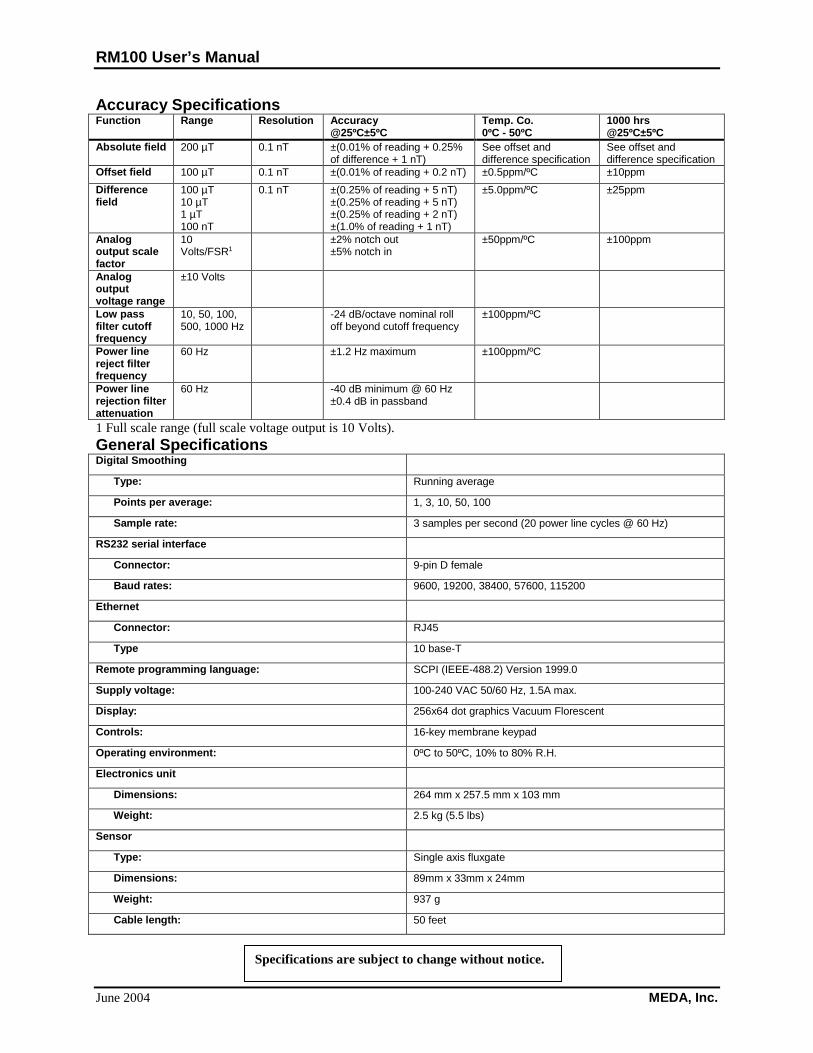
RM100 User’s Manual
June 2004 MEDA, Inc.
Accuracy Specifications Function Range Resolution Accuracy
@25ºC±5ºC Temp. Co. 0ºC - 50ºC
1000 hrs @25ºC±5ºC
Absolute field 200 µT 0.1 nT ±(0.01% of reading + 0.25% of difference + 1 nT)
See offset and difference specification
See offset and difference specification
Offset field 100 µT 0.1 nT ±(0.01% of reading + 0.2 nT) ±0.5ppm/ºC ±10ppm Difference field
100 µT 10 µT 1 µT 100 nT
0.1 nT ±(0.25% of reading + 5 nT) ±(0.25% of reading + 5 nT) ±(0.25% of reading + 2 nT) ±(1.0% of reading + 1 nT)
±5.0ppm/ºC ±25ppm
Analog output scale factor
10 Volts/FSR1
±2% notch out ±5% notch in
±50ppm/ºC ±100ppm
Analog output voltage range
±10 Volts
Low pass filter cutoff frequency
10, 50, 100, 500, 1000 Hz
-24 dB/octave nominal roll off beyond cutoff frequency
±100ppm/ºC
Power line reject filter frequency
60 Hz ±1.2 Hz maximum ±100ppm/ºC
Power line rejection filter attenuation
60 Hz -40 dB minimum @ 60 Hz ±0.4 dB in passband
1 Full scale range (full scale voltage output is 10 Volts). General Specifications Digital Smoothing
Type: Running average
Points per average: 1, 3, 10, 50, 100
Sample rate: 3 samples per second (20 power line cycles @ 60 Hz)
RS232 serial interface
Connector: 9-pin D female
Baud rates: 9600, 19200, 38400, 57600, 115200
Ethernet
Connector: RJ45
Type 10 base-T
Remote programming language: SCPI (IEEE-488.2) Version 1999.0
Supply voltage: 100-240 VAC 50/60 Hz, 1.5A max.
Display: 256x64 dot graphics Vacuum Florescent
Controls: 16-key membrane keypad
Operating environment: 0ºC to 50ºC, 10% to 80% R.H.
Electronics unit
Dimensions: 264 mm x 257.5 mm x 103 mm
Weight: 2.5 kg (5.5 lbs)
Sensor
Type: Single axis fluxgate
Dimensions: 89mm x 33mm x 24mm
Weight: 937 g
Cable length: 50 feet
Specifications are subject to change without notice.


