RN-24. May l<J(>5

CO

Q

n

rVECTRO-OPTICAL. ays

f INC. '

©TE®

TURBULENT MIXING IN THE BASE FLOW REGION

Hartley H. King iind M. Richard Denison

mmi m

-.-. t^". ^^vi: ---v.r":.. --■■ - - - - ̂ ^ »M ^-t

_. , _. . .^ r ■-

.--;■-:- ~S ffj^m^lBpiL-—. .a-i^lff ..' -

■ '•" '-••■iTii^ä?!^p~-7nfcT ■ ■-^--^f^* ^ "-■Ea-3; - :j7-

: •:. : :.. > ;!

f//*«^*/ douti ftom the Miidk ^^ %r« «y*^ jr)fer*<^ «wettpüspßiative

vl the torn elemms in tlimäß0^^ Modern science has since identijied these four ehmentsuith the^o* stäteti* v&eh

matter appears in the trntverui ga, Uqtd0&^ir^ui plasma. Understanä'wg the

properties of matt€rint)^^,fßhm0

I r r

_> v

• r i

r r r

|

r r ; \

I r :

r r f

EOS Research Note No, 24, May 1965

TURBULENT MIXING IN 7/7/ BASE ELOW REGION

Hartley IE Kh/" </;/<7 M. Richard Denisoii

1

I I I

E m s

ELECTRO-OPTICAL SYSTEMS, INC. Pasadena, California

A Subsidiory of Xerox Corporation

V

SUMMARY

An exploratory study is made in connection with the problem of pre-

dicting properties of the turbulent base flow region of a body at hypersonic

speeds. An attempt is made to calculate the gross features of the base flow

using a non-similar mixing model including the Chapman-Korst recompression

condition. The expression for the eddy viscosity is based on a model which

allows the turbulent equations to be transformed into incompressible laminar

form. The empirical factor in the eddy viscosity expression is evaluated

from data obtained from the near field (in the linear growth region) of jets

exhausting into a quiescent region. The same expression for the eddy vis-

cosity is then used in an attempt to estimate the growth of non-similar

turbulent mixing layer using both turbulent and laminar initial profiles.

The correlation of turbulent jet mixing data for speeds up to Mach 3

fhows that the eddy viscosity is » -very strong function of Mach number (or

of density ratio across the jet, since the data are for adiabatic flow).

If the eddy viscosity dependence on density ratio persists for density

ratios typical of re-entry conditions, then it is found that at these

conditions the growth rate of the turbulent shear layer is orders of magni-

tude slower approaching the rate of growth of the laminar mixing layer

under the same conditions. This is in maTked contrast to the situation

at low supersonic speeds, where the turbulent mixing layer dividing stream-

line velocity approaches the similar value well before recompression occurs.

If this speculation is correct, then the stagnation enthalpy at recompress-

ion in the hypersonic turbulent base flow should be well below the total

enthalpy value, since the enthalpy build-up on the dividing streamline

will be similarly suppressed.

This research is a part of PROJECT DEFENDER, sponsored by the Advanced Research Projects Agency, Department of Defense, under ARPA Order No. 254-62, monitored by Air Fcrce Ballistic Systems Division under Contract No. AF 04(694)-570.

EOS RN-24, 5-6 5

I

I I

r

r

r r

r

r !

i i i

i i

TABLE OF CONTENTS

Page

1, INTRODUCTION 1

2. EDDY VISCOSITY 2

j 3. CONSERVATION EQUATIONS 5

4. SIMILAR SOLUTION 9

5. CORRELATION WITH EXPERIMENT 11

m 6. NON-SIMILAR SOLUTION 13

7. LAMINAR INITIAL CONDITIONS 17

8. TRANSFORMATION INVERSION - LAMINAR BODY 18

9. TURBULENT INITIAL- CONDITIONS 20

10. TRANSFORMATION INVERSION - TURBULENT BODY 27

11. NUMERICAL SHEAR LAYER CALCULATIONS 28

12. BASE FLOW OF CONE OR WEDGE 30

13. RESULTS FOR 10° CONE 33

14. CONCLUDING REMARKS 36

REFERENCES 3,

APPENDIX A 40

APPENDIX B 41

EOS RN-24, 5-6 5 iii

ILLUSTRATIONS

1. Mixing Layer Regions

2. Geometry of the Jet Mixing Experiment

3. Experimental Dividing Streamline Velocity Calculated from Mass Balance

4. Correlation of Profile Data

5. Correlation to Determine the Eddy Viscosity Factor k-

6. Equivalent Skin Friction Coefficient

Cr for Cones and Wedges, H /H =0 f 6 ' w e

7. Equivalent Skin Friction Coefficient

C, for Cones and Wedges, H /H =1 f ^ ' w e

- i 7 8. Effect of Wall Enthalpy Ratio on C for R = 10

9. Turbulent Initial Mixing Layer Profile

10. Development of the Velocity Gradient Profiles with Streamwise Distance

11o Development of the Enthalpy Function W Profiles with Streamwise Distance

12. Velocity on the Dividivig Streamline

13. Enthalpy Function W on the Dividing Streamline

14. Relation Between x* and S*

15. Shear Layer Momentum Thickness Integral

16. Base Flow Model 51

17. Dividing Streamline Velocity Before Recomnression 51

18. Recirculating Region Enthalpy 51

19. Effect of Mach Number on Centerline Static 52 Enthalpy After Recompression

20. Effect of Reynolds Number on Centerline Static 52 Enthalpy After Recompres.sion

21. Effect of Mach Number on Base Pressure 52

Effect of Reynolds Number on Base treasure 52

A4

44

44

45

45

46

46

46

46

47

48

49

49

50

50

EOS RN-24, 5-65

[

1

[

[

r r

i

i

i

i

i

ACKNOWLEDGEMENT

The authors wish to express their appreciation to

Dr. Eric Paum for providing the computer program for

calculation of the non-similar mixing layer profiles

of this report.

EOS RN-24, 5-65 vii

1. INTRODUCTION

Predictions of observables in the wakes of slender re-entry vehicles

have been found to depend crucially on the flow properties assumed at

the neck region. For example, predicted electron densities and radar

cross-sections of wakes may vary by orders of magnitude, depending on

the assumed value oi the centerline neck enthalpy ratio h/H . Since CJ e

properties at the wake neck are determined by the flow processes in the

body boundary layer and base flow mixing regions, it is clear that

accurate methods for flow calculations in these regions must be developed.

The primary objective of the present, paper is to devise a procedure

for calculating the gross properties of the hypersonic turbulent base

flow (e.g. base pressure, neck enthalpy, etc.). The problem is approached

Trom the point of view of the generalized Chapman-Korst base flow model, (2 3)

as was done in the laminar case. ' For laminar flow this model is

thought to be reasonable for moderate supersonic Mach numbers, but is

probably not adequate for re-entry conditions, Recently, Reeves and (4) (5)

Lees, Webb, Golik and Lees, and others have attempted to devise

base flow models more applicable to re-entry conditions. These methods

are not yet well established and still may not contain essential features

even for the laminar case. For turbulent flow the difficulty is compounded

by uncertainties related to the "eddy" transport coefficients, so it

seems more reasonable to use the simpler Chapman-Korst model at the

present time. If this procedure is adopted, then what remains is to

develop a reasonable empirical model for the eddy coefficients. A major

pare of the present paper is devoted to this task.

Having developed appropriate expressions for the eddy coefficients,

one can then solve the non-similar mixing layer equations4 an: thereby

determine how rapidly the profiles change from the initial distributions

on the body at separation to the fully-developed profiles far downstream

EOS RN-24, 5-65

from separation. For the base flow this rate of change or build-up of

the profiles may be of crucial importance if recompression occurs before

the asymptotic or fully developed condition is approached. This is the (2 3)

situation occurring in laminar case, and could also occur in the

turbulent case.

The present report contains three separate parts. The first shows

that experimental turbulent mixing data can be correlated by an eddy

viscosity model based on the assumption that pc - function of x only.

Thus the effect of compressability is taken into account in the same

manner as with laminar flow; the effect of turbulence thereby being

placed in the streamwise variable transformation. The second part of

the report deals with the solution of the non-similar mixing layer

problem, assuming that the previously developed expression for the

eddy viscosity .emains valid even near the separation point. The third

portion of the report utilizes the results of the non-similar mixing

layer analysis and the Chapman-Korst base flow model to predict the

base flow properties of a highly cooled slender cone under re-entry

conditions.

As might be expected, the results of this report depend crucially

on the expression developed for the eddy viscosity. Unfortunately, the

available data cover a vei-y limited Mach number range and are for

essentially adiabatic flow, so that a considerable extrapolation is

involved in applying the model to the re-entry case. Thus the final

base flow results presented must be considered tentative and subject

to revision when new turbulent mixing data become available.

EOS RN-24, 6-6 5

i

2. EDDY VISCOSITY

A fundamental assumption of this report is that the compressible

mixing layer flow can be transformed to an equivalent incompressible

flow. The transformation is of the type used by Ma^er, Burggraf (8) Ting and Libby and nthers, in which the stream function and shear

stress over a mass element are assumed invariant, In the incompress-

ible plane the eddy viscosity is assumed to be given by Prandtl's (9) expression, and is proportional to the width of t^e mixing «one

and the velocity difference across the layer. Ferri recently has

argued that when generalized to compressible flow, Prandtl's expression

should be proportional to the tangential mass flux difference instead

of the velocity difference. For mixing layers with negligible flow

on the inside both expressions are identical. A more serious defect

is that the eddy viscosity is assume^ to suddenly change from a form

suitable to the body boundary layer to that characteristic of the

mixing layer after the shoulder expansion.

With these assumptions the resulting compressible eddy viscosity

is the following: i

€ = K — Ue D (1)

In Eq, (1) k is a dimensionless proportionality factor to be deter-

mined by correlating the theory with experimental data and is fit most

a function of the external flow conditions. The quantity b is a

suitably chosen width of the mixing layer and p is a reference

density used to give e the dimensions of viscosity. As pointed out

by Ting and Libby, Eq. (1) implies that e is variable across the mix-

ing zone because of the density variation, whereas in the incompressible

case it is constant. For the mixing layer the width is assumed to be:

EOS RN-24, 5-6 5

b = 6 = \ u*a-u*) -^ dy (2a)

so that e Is proportional to the momentum thickness of the mixing

layer. We could also try for the width

b = \ -^ dy (2b)

where (by convention) y. and y are respectively the values of y where 2

u* = 0.1 and 0,9. It turns out that Eqs. (2a) and (2b) produce

essentially the same final results for a mixing layer of negligible

initial thickness. For the more general problem however, Eq# (2a)

seems more lensonable than (2b). The only justification for these

assumptions for b at present is that they simplify the analysis some-

what by uncoupling the energy terms from the momentum equation. As

with all turbulent theories of this type, further justification for

the selection of the expression for e must come by comparing the

results of the analysis with experimental data.

EOS RN-2A, 5-65

I

I 1

I I I I

I

1 I

i

I I

I

3. CONSERVATION EQUATIONS

The boundary Layer equations involving the me^n flow variables «re

assumed to be appropriate for the description of the constant pressure

mixing region (Fig. 1), provided the exchange coefficients are replaced

by their empirical turbulent counterparts. In spite of the well recog-

nii-'id fact that er tgy, species, and momentum transport may occur by

different mechanisms in turbulent flow, we simplify matters by assuming

that Fr = Le = 1. Then only the eddy visccs.vy is used explicitly.

This rough model later may be refine* the results prove prot ing.

The equations are:

(puro:l)x + (pvro

J)y = 0 (3a)

puu + pvu - (cu ) (3b) x y y y

puH + pvH = (PH ) (3c) x y - y y

where r - r (x) is the mean radius of the thin mixing layer in the o o ' e> j

axisymmetric case. The boundary conditions are (Fig. 1) :

y - - <x>: u = 0, H = H (constant) (4a)

y = *>: u = u,H=H (4b) e e

y = 0: v = 0 (dividing streamline) (4c)

x = 0, y > 0: u ■ given initial velocity profile (4d)

H = H - (H - H ) (1-u*) (Crocco Integral) (4e)

EOS RN-24, 5-6S

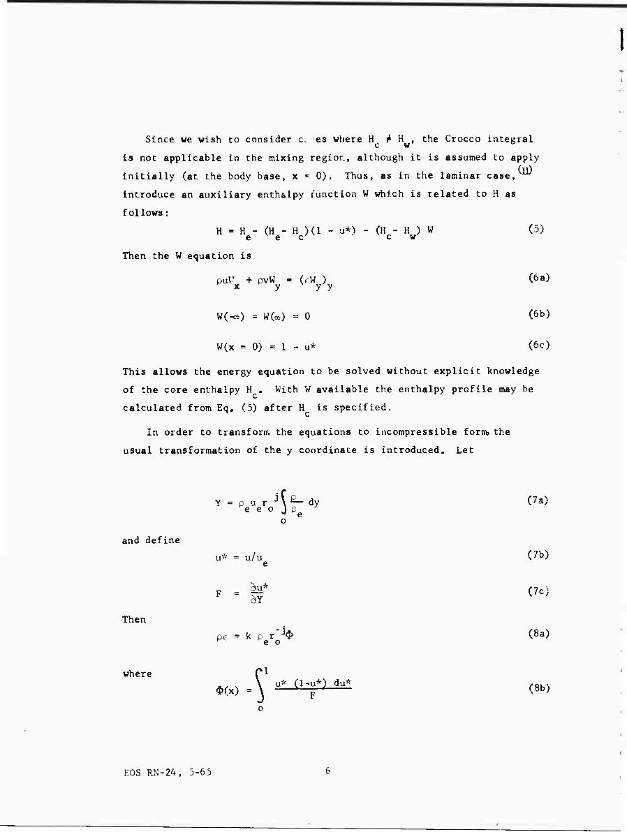
Since we wish to consider c. es where H jt H , the Crocco integral

is not applicable in the mixing region, although it is assumed to apply

initially (at the body base, x = 0). Thus, as in the laminar case, ^

Introduce an auxiliary enth&lpy /unction W which is related to H as

follows:

H = H - (H - H )(1 - u*) - (H - H ) W (5)

Then the W equation is

puV + pvW = (rW ) (6a) x y y y

W(^=) = W(co) - 0 (6b)

W(x = 0) = 1 - u* (6c)

This allows the energy equation to be solved without explicit knowledge

of the core enthalpy H . With W available the enthalpy profile may be

calculated from Eq, (5) after H is specified.

In order to transform the equations to incompressible form, the

usual transformation of the y coordinate is introduced. Let

j(ß-dy (7a) J p0

Y = p u r e e o ._e o

and define

Then

u* = u/u_ W

v . 2"* (7c) F " ÖY

pe - k P v'h C8a) v- e o

where \ u* (1-u^ o * y F

) du^ = \ -' ^jp — (8b)

EOS RN-24, 5-65

I I

Introduction of relations (7) and (8) in the conservation equations (3)

and further transformation to Crocco coordinates yields

U* S = ^eU»roJk ^ F2 ?2 <9) ^x e . o ^t

and a similar expression for W. The factor in parentheses on the right

hand side depends on x only, although $ depends upon the solution.

Therefore Eq. (9) can be put in the form of the laminar momentum equa-

tion if we define

dS-- = Fw2 (Peuero

Jk *) dx (10a)

F* = F/Fw (10b)

where F Is the value of F on the body before separation.

Then the conservation equations become

2 u* r^— ■ F* " (\\a}

* ^H „,,.2 Ö_W . . U ÖS* = F ~2 <llb)

du"

These equations are in a form identical to the laminar equations and

also have the same boundary conditions as in the laminar case. The

differences are in the inversion of S* back to physical space and in

the initial conditions. If the body boundary layer is turbulent,

initial conditions for the mixing layer must take this into account.

On the other hand it is conceivable that the body boundary layer might

be laminar with transition occurring at the shoulder. In this case

the initial profile wiH also correspond to the laminar case.

EOS RN-24, 5-6 5

For a lauiinar body boundaiy layer the initial and boundary condi-

tion are;

S* = 0: FnO.u*) = f W/f,!B<0) (12a)

W(0,u*) = 1-u* (12b)

u* - 0: F*(S*,0) = W(F*,0) = 0 (12c)

u* « 1: F*(S*,1) = W(S*,1) = 0 (12d)

where f" Is obtained from the Blaslus solution (see Section 7).

(11) These equations have been previously solved and the solution tabulated.

The problems remaining, then, are the inversion of the turbulent

flow transformation S* back to physical space and establishment of

initial conditions for turbulent flow on the body.

EOS RN-24, 5-65

I

I I I

I i

i

I *

I I

A. SIMILAR SOLUTION

A first step in inverting the turbulent solution is to obtain the

parameter k from experiments. For this purpose we investigate similar

solutions which can then be compared with experimental data. It is

known from the laminar case that at large values of S* the effect of

the initial structure of the shear layer will disappear and the solution

will asymptotically approach the similar solution of Chapman.

Since Che turbulent problem has been made mathematically equivalent to

the laminar case with the exception of initial conditions, the asymp-

totic solutions must be identical.

In order to obtain the Blasius equation instead of its counterpart

in Crocco coordinates we introduce the normal distance parameter

(25*) '

Then the velocity is assumed to be a function of TJ only

u* - f'Crj) (13b)

When Eqs. (JJö) and (i3b) are introduced in the conservation equations

the familiar results are obtained.

f + ff =0 (14a)

w + fw =0 duh)

The boundary conditions are f (-<») = 0, f (*>) «= 1, W(~ac,) = W(-x) ■ 0,

and f(0) = 0, The last condition follows from the specification that

EOS RF 24, 5-6 5

rj = 0 corresponds to the dividing streamline. Clearly the solution for

W is W = 0, which of course implies the usual Crocco integral relation

for the total enthalpy from Eq. (3). The solution for f may be obtained

from tabulations by Chapmanv and Christian

The momentum thickness function for the similar solution is given by

1/2 * = "^p c (15a)

w

where

f'd-f) dt) = ,8756 (15b)

-00

Use of Eq, (15) in Eq, (10) and integration yields:

(2S*)1/2= k c F \ p u r jdx (16a) w 1 e e o

Hence

where

n = -4- (i6b)

\ p u r jdx = (2S*)1/2/ " = k c \ pur Jdx = (2S*) /F (16c) j e e o w

It can be seen from Eqs. (I6b) and (16c; as well as the definition

of Y, Eq. (7a), that the similarity parameter r\ becomes proportional

to y/x for a two dimensional incompressible flow, which is a well

known behavior.

EOS RN-24, 5-6 5 10

I

i I I

5. CORRELATION WITH EXPERIMENT

The primary source of correlation is obtained from experiments

dealing with the turbulent flow of jets exhausting into a quiescent

region (Fig. 2). The region most applicable to the problem of the base

flow is the mixing zone between the jet exit and about five diameters

downstream. This type of flow is "inside-out" compared with the base

flow problem, since the high velocity flow is inside the mixing region

rather than outside. This hopefully will not make any difference, so

that if the jet experimental data can be correlated with the theory,

then the theoretical results can be applied directly to the base flow

problem.

The primary source of data for the eddy viscosity correlation of (14)

this report is the work of Maydew and Reed, who measured velocity

profiles in the near mixing region of turbulent jets exhausting into

the atmosphere. The nozzle exit diameter of these experiments was 3",

and profile data were obtained for exit Mach numbers ,7, .85, .95, 1.49,

and 1.96 at five axial stations in the range 1,5" < x^ll^", Leipmann

and Laufer also give data for MR=.05, while 5ome earlier data of

possible applicability to the present problem are referred to by Maydew

and Reed,

One result which can be compared with the theory is the velocity

on the dividing streamline. According to the solution of Eq, (14«) this

value should be u* = .587 if the flow is sufficiently downstream of

separation for similarity to hold. In order to check this result, the (14) jet mixing profiles of Mayd»/and Reed were integrated outward from

the axis of the jet until the mass in the profile was equal to the mass

flowing throv. '^e jet. In these calculations the Crocco integral

relation was used to calculate the density variation, and the entrance

mass was calculated from the measured stagnation temperature and

pressure, assuming an isentropic one-dimensional expansion. Further

details regarding this mass balance are given in the Appendix.

EOS RN-24. 5-65 11

Flg. 3 shows the calculated results of the mass balance for the five

exit Mach numbers of the experiments of Maydew and Reed, One sees that

the calculated experimental dividing streamline velocity u* is about

0,6 or perhaps a little higher. It is substantially independent of

streamwise distance for x/d > 1, indicating that the mixing region has

probably reached similarity. It should be noted, however, that the

accuracy of the integration procedure is very poor for stations close

to the jet exit, since most of the mass flow inside the dividing stream-

line is in the potential core and not in the mixing profile (see Fig. 2).

UnJer these conditions a small error in the mass flow calculation will

produce a large error in the value of u* on the dividing streamline.

Further, the use of the Crocco integral for the density variation may

be questioned. We therefore conclude from Fig. 3 that the dividing

streamline velocity data agree with the present theory within the

possible error of the measurements and integration procedure, but these

data are prcoably too crude to constitute a critical test.

The second and more important portion of the data correlation concerns

the fitting of the theoretical velocity profile to the data. This has

traditionally been done by finding the best numerical value of the

"spreading parameter" a such that the velocity profile is represented by

u* = g(o p (17)

where g is a profile function specified beforehand. For example, the

error function profile is frequently used, while Maydew and Reed find

that the data correlate well with the results of Crane. The numeri-

cal value of o for "best fit" of course depends on the choice of profile,

rt certain arbitrariness also exists in the selection of the profile

position from which y is measured, and this traditionally is taren as

the location where u* = ,5 for the data.

>

i

EOS RN-24, 5-65 12

1 I I I I I I I

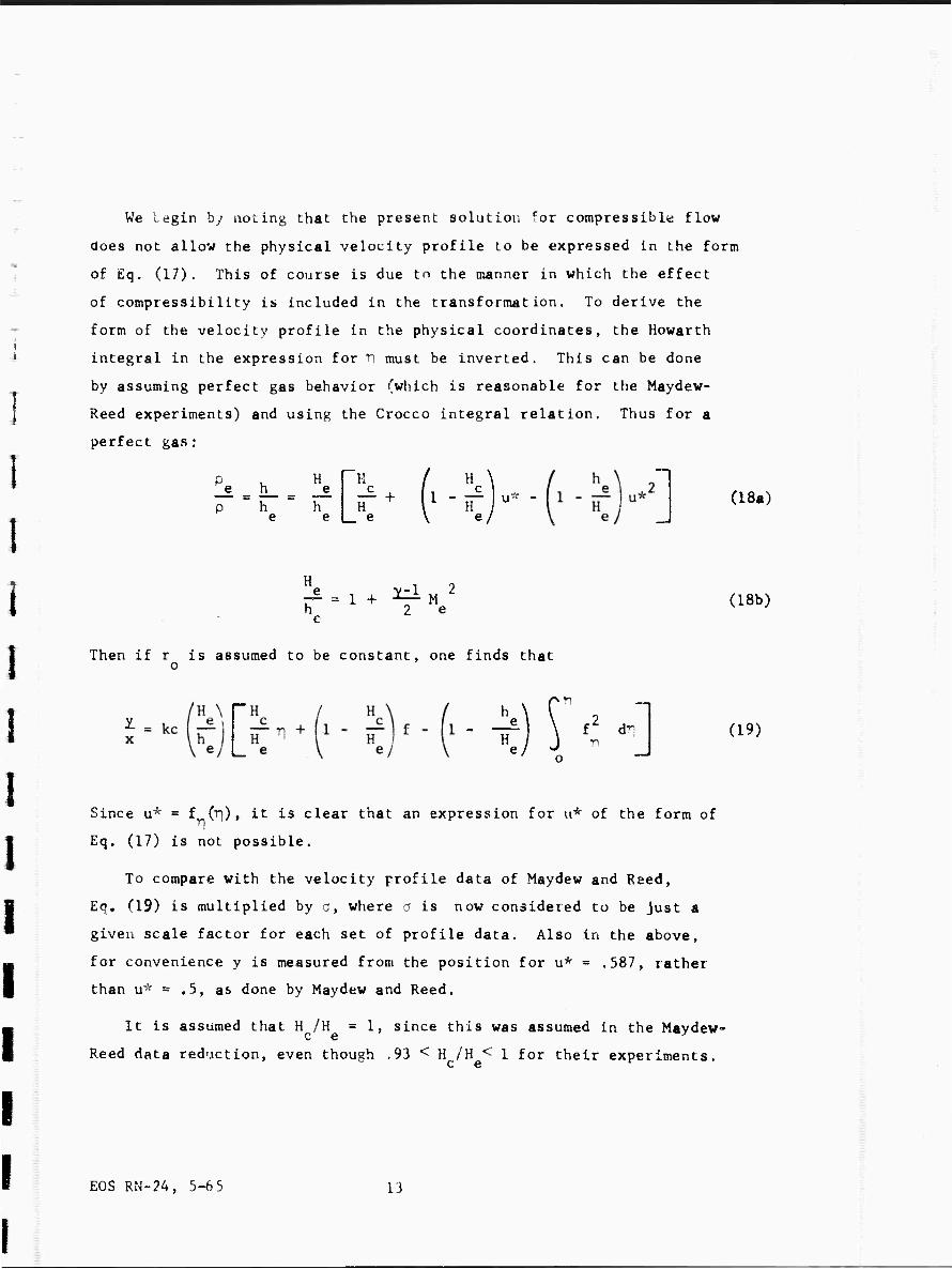
We 1 egin by noting that the present solution ''or compressiblt; flow

does not allow the physical velocity profile to be expressed in the form

of Eq, (17). This of course is due to the manner in which the effect

of compressibility is included in the transformation. To derive the

form of the velocity profile in the physical coordinates, the Howarth

integral in the expression for "H must be inverted. This can be done

by assuming perfect gas behavior (which is reasonable for the Maydew-

Reed experiments) and using the Crocco integral relation. Thus for a

perfect gas:

h_ h

H

e L_ e

H + 1 (18a)

H , o, e = ! + 1^1 M 2

h 2 e c (18b)

Then if r is assumed to be constant, one finds that o

L ..

. n

d^l (19)

Since u* = f (r\) , it is clear that an expression for u* of the form of

Eq. (17) is not possible.

To compare with the velocity profile data of Maydew and Raed,

Eq, (19) is multiplied by a, where a is now considered to be just a

given scale factor for each set of profile data. Also In the above,

for convenience y is measured from the position for u* ■ .587, rather

than u* = .5, as done by Maydew and Reed.

Re

It is assumed that H /H =1, since this was assumed in the Mavdew- c e '

ed data reduction, even though .93 < H /H < 1 for their experiments. c e

EOS RN-24, 5-6 5 li

Also x = x + Ax, where x is the experimental distance from the jet e e

exit and Ax is an additional incremental d?st. nee to the "virtual origin" (14)

of the turbulent mixing layer as tabulated by Maydew and Reed,

Fig. 4 shows the correlation of the Maydew-Reed data with the Chapman

profile for the various experimental Mach numbers. The constant k was

first obtained by finding the "best fit" of Eq. (19) with each set of

profile data, using a "le> t squares" analysis, (Note that the momentum

thickness factor c = ,8756 from the Chapman solution,) The theoretical

curves shown, however, are based on the final equation for the correla-

tion constant, as described below. It is seen that the shapes of the

profiles seem to correlate quite well. This is perhaps not too surpris-

ing, however, since many curves of this general shape seem to correlate

in a reasonable manner it the adjustable constant is properly chosen.

It was hoped initially that the quantity k would not be a function

of Mach number, but would be a universal constant. Instead it is found

to vary quite strongly with Mach number for .05 ^ M s 3. It is reason-

able to assume that this variation is related to the density ratio

across the mixing region p /p . For a perfect gas this is equal to

H /h , and if the flow is completely adiabätic, then p /p = H /h = ce.,, ecee v— Z

(1 + ■'y^ M ). Figure 5 shows a log-log plot of k as a function of

p /p , assuming adiab&tic flow. Based only on the Maydew-Reed data,

it is found that very nearly

b = ,0606

b2 - 2.0

If the data of Leipmann and Laufer and tentative data of Zumwalt

(see Appendix) had been included in the correlation, the constants in

Eq. (20) would probably be changed slightly. Thus for the similar

solution: / * b.

(20)

(21)

Comparing this with Eq, (1), it is seen that a more reasonable reference 2 2

density probably would have been p rather than o

EOS RN-24, 5-65 14

i

I I

8

I

6. NGN-SIMILAR SOLUTION

Equation (21) xs a plausible form for the eddy viscosity, which

should be applicable at least to fully-developed, i-.early adiabatic

turbulent mixing for Mach numbers up to about 3. The justification for

its use lies in the fact that experimental data correlate well with theory,

Application of this equation at higher Mach numbers, for highly cooled

mixing layers, or in the non-similar region close to the separation point

(Fig. 1) obviously may be improper. Because of the urgent need for some

sort of theoretical description of turbulent mixing under these condi-

tions, however, the extended use of Eq, (21) is proposed. Any conclusions

based on this model must of course remain tentative for conditions out-

side of the established correlation range.

We now propose to solve non-similar Eqs. (11) using Eq. (21) f"r ti-e

eddy viscosity. We introduce the correlation in the x coordinate trans-

formation for the non-similar case.

S* = Fw2 \ peVTroJ dx ^22a)

where

MT = k $ (22b)

( 2} Comparing Eq, (22$ with the well-known laminar expression for S*,

we see that the term Li„ replaces the laminar viscosity u times r . i " e o

Thus the relative growth rates dS-'/dx of turbulent and laminar mixing

layers (in the two-dimensional case; are directly related by the ratio

!' Ai • One sees that if the eddy viscosity is in fact representaMe

by Eq, (21) over a wide range of conditions, then the density ratio

EOS RN-24, 5-65 15

across the mixing layir (p /p ) is extremely important in determining the

growth of the turbulent mixing 1ayer. It has already been shown thai,

the conse-vation equations have been converted to laminar form in Eqs, (ll)

Eqs. (22) provide the transformation of Sx back to phys-cal space. In

essence what has been accomplished, therefore, is the placement of the

turbulent effects into the coordinate transformations. One should thus

be able to obtain universal solutions to Eq. (11) which depend only on

the shape of the initial profile F(0,u"), just as in the laminar case.

The task that remains is to obtain the initial mixing layer profiles

by soIvin3 the boundary layer on the body surface upstream of separa- (2 3) tion. Eqs, (11) will then be solved by a finite difference method. ' *

The simplest case to consider is that for laminar flow on the body sur-

face, which is a limiting situation which might correspond to the occur-

rence of transition at the separation point. A slightly more difficult

but still tractable problem occurs for fully developed constant pressure

turbulent flow (i.e. cone or wedge). The calculations of this report

are restricted to these cases.

EOS RN-24, 5-65 16

I

I I I

7. LAMINAR INITIAL CONDITIONS

For laminar flow on the body it is found that Blasius solution is

applicable. Thus ac the separation point:

f" (u*) F(0,u*) = : (23a)

u* = f W (23b)

^ r M A e o \ pdy % " ^- \ (23c)

S = \ C. p u u r 2jdx (23d) w \ be e e o

bod y

C, = pu/p U (Chapman-Rubesin constant /__ , b e e c \.u u J \ C23e) for the body)

In (23a) and CcJb) prime denotes dif ferentiatior. with respect t« (2) the Blasius variable TI_. As in the laminei mixing case we let:

Fw = f,V0)/^\ C24a)

£'^(0) = .4696 (24b)

The initial condition for the energy equation is W = 1-u*, since

the Crocco integral is assumed to apply to the flow on the body surface.

EOS RN-24, 5-6 5 17

8. TRANSFORMATION INVERSION - LAMINAR BODY

The calculation of S* is now considered. From Eq, (22), we are led

to the following differential equation:

■— = Jp u F kr j"W (25a) dx I e e w o : K /

{ 1

$*(S*) = Fw^ - \ u*(l-u*) ^ (23b)

Define a new variable x* by the following relation

e'ew o * = \ PQUDFTk r^

Jdx (26)

o

Then Eq, (25a) may be written

dS* ~~; = **(S*) S*(0) = 0 (27)

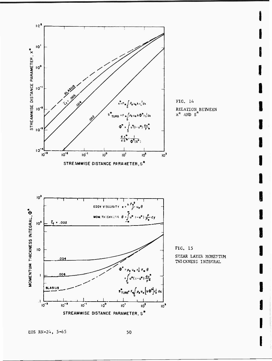
This equation was integrated using the function data for Q* from the

shear layer solution, and the resulting function x>v(S") is given in

Fig. 14, The relation between S* and physical x is therefore obtained

from Eq, (26) and the function x^S*) .

For comparison of turbulent mixing with the laminar mixing case,

it may be desirable to express the turbulent solution in the laminar

variables. For this we need to calculate S** for the turbulent case,

where

S** = S/S w

f 2^ S » \ C p u u r Jdx (28)

l m e e ~ o v ' -'o

ECS RN-24, 5-65 18

and C is the laminar Chapman-Rubes in constant for the mixing laver. m

Then the rate of build-up of transformed length scale ratio S** with

respect to x* is given by:

dS*-* dx*

C n^

k F S w w

(29)

The bracket term in Eq. (29) is a constant for a given body at given

flow conditions. The value of this constant in a base flow depends on

the details of the "matching," which is carried out using the Chapman-

Korst recompression condition. For two dimensional flow the laminar

length variable S** is proportional to x*(S*) , but for axisymmetric

flow the radius factor enters explicitely. Further discussion of the

laminar-body, turbulent-mixing-layer problem is deferred until later.

i

1

i

i I

I EOS RN-24, 5-6 5 19

9. TURBULENT INITIAL CONDITIONS

For a turbulent body boundary layer we need to obtain new initial

conditions which replace Eq. (23) in the analysis of the preceding

sections. In spite of the great effort which has been devoted to

research on turbulent boundary layers, there still does not exist a

well established theoretical method to obtain compressible turbulent

boundary layer profiles. The most recent and promising method appears ^ 17)

to be the transformation method of Coles,v as further explained by ( ig)

Crocco.' Thus a transformation will be found which (hopefully)

establishes a correspondence between a known incompressible flow and

the desired compressible flow. The incompressible profiles (which are

established by a semi-empirical method) are thereby transformed to the

compressible flow.

Let "barred" symbols refer to the transformed incompressible flow

and unbarred symbols represent the compressible flow. The aim of the

Coles transformation is to find the quantities a(x), •q (x), and 5(x)

defined as follows:

r *j 2 f£4^(x) r

Ol

* } ,J{ = a(x) (30a) .(x,y)

(x) (30b) P äy '•

dx -, , d^'W OOc)

EOS RN-24, 5-65 20

.'heie the stream functions are:

y

''O

j, = r j - pu dy (30e) 0 J

o

(The quantity of cr Eq, (3Ua) is not related to the jet-mixing o of

Fig. 4.) Restricting attention to the cpse of zero pressurr gradient.

Coles and Crocco find that

u u e ri /" J i \ — = i— =■- -L = constant \J*■ ' u u c

e

The relation between the wall shear stresses is

T ^ p U C p U W W W L C € /1 O \

T ~ ~ p u = Z 2 v* w n w w o^p u 1 f e e

? where Cc- x /(p u /2) is the usual skin friction coefficient. Coles

r w e e introduces the idea of a turbulent substructure, which yields for a

the result

- \L . \L- l**M (33) i l ■

S ^w/VJs]

where u is a mean substructure viscosity, obtained from the hypothesis

of a constant substructure Reynolds number. ' 'From Eq. (31) to (33)

we obtain

2 _ Cf / Mw « ;=i^;i~;

EOS RN-24, 5-65 21

For the case of Pr = 1 the Crocco integral relation holds on ttu body.

Then if laminar viscosity is a^sumed proportional to static enthalpy,

the following generalization of Coles' results (Coles' Fq. 4.17 for

u, /u is obtained: s w

Hi.

V1

c"f 2

7.5

ai

/H - H \ e w |

\ w /

a2= 305

Öf 2

_J (3 5a)

(35b)

It is further consistent within this framework to use the approximation

P H e w

P = h w e

(36)

So that from Eq. ( 34) :

= ■

H

r+N - a. H - h e e

M 2

H \ e (37)

The simplest way to treat the compressible turbulent boundary layer

using this formulation is to specify C (i.e. work the problem backwards

by specifying the equivalent incompressible skin friction coefficient).

Then the compressible skin friction is given by Eq, (37), and the com-

pressible heat transfer is obtained from the enthalpy gradient using

the Crocco integral. What remains to be done, then, is to find the

relation between the compressible and incompressible length scales

(i.e. Reynolds numbers). Then the compressible velocity profile can

be expressed in terms of a given incompressible profile corresponding

to the specified C .

Rather than finding the "elation for C(x), we instead seek a direct

relation between C- and the curopressible length x. If the Coles-Crocco

EOS RN-24, 5-6 5 22

transformation relations are substituted in the compressible momentum

integral relation, it is found that

■'.x -pur Jx = w e o (38a)

P u R = -~- \ u* (1 - u*) dy e^ I- e |a o

(38b)

The incompressible momentum thickness Reynolds number R is ee related to Cf by a relation based on the law of the wall. Let the In-

compressible velocity profile in this region be given by (Ref, 19,

page 140):

u_

u

i u y i- in -4- + c (39a)

Y w " v 7

2 (39b)

where according to Coles, ^K = ,4 and C = 5.1. Then from Eq. (38b)

it is found that

-KC

eQ K

7 0 O

e (1 - T) + (1 + 7) (40a)

where K (40b)

\i5f/2

! -4

\

I I

By using Eq, (40) and (35), Eq. (38) can be integrated along the body

from the point of transition to the uase. If Z is assumed to be very

large, then the integration is easy to carry out. Assuming that transi-

tion occurs at the nose, the final result nay be put into the standard form;

EOS RN-24, 5-6 5 23

JL

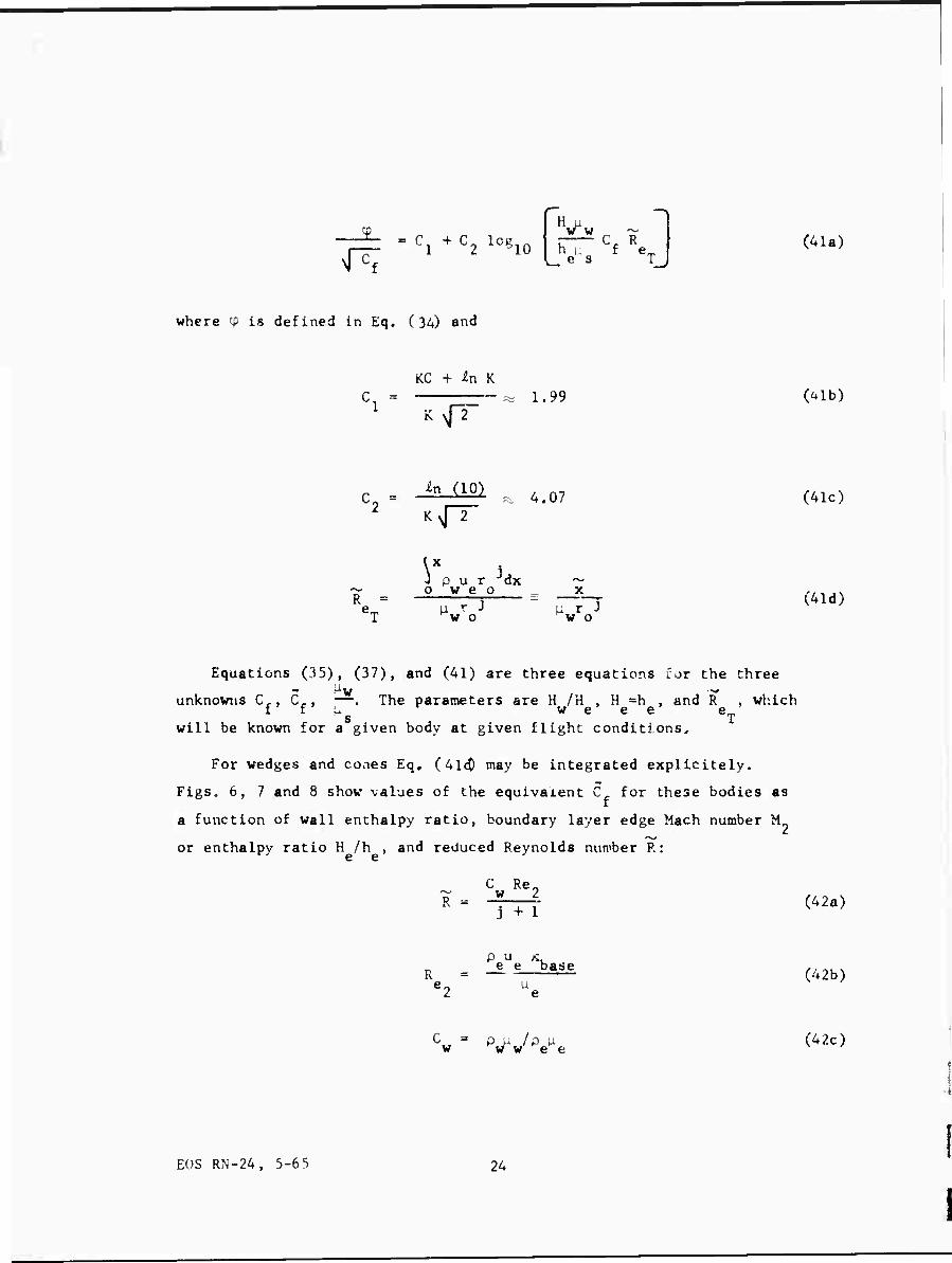
f^ = C1 + C2 log10

H u —Z C, R h u f e^ es T

(41a)

where cp is defined in Eq. (34) and

ci-

KC + ^n K

K {T 1.99 (41b)

C2 = ^n (10)

Kvpr 4.07 (41c)

R = \ Pur dx o w e o

w o [i r J w o

(41d)

Equations (35), (37), and (41) are three equations for the three

unknowns C,., C,, —. The parameters are H /H , H =h , and R , which ffu weee e

will be known for a given body at given flight conditions.

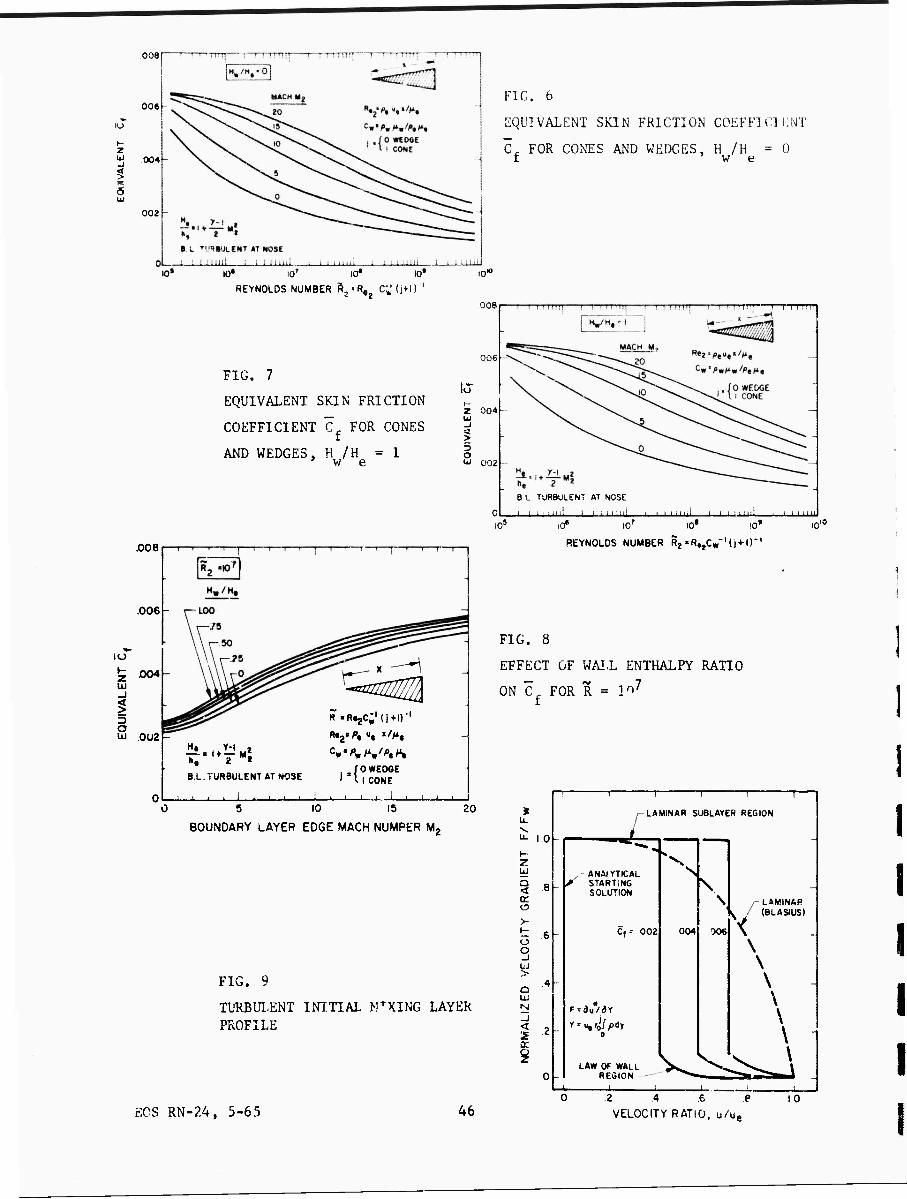
For wedges and cones Eq. (4l4) may be integrated explicitely.

Figs, 6, 7 and 8 show values of the equivalent C for these bodies as

a function of wall enthalpy ratio, boundary layer edge Mach number M9

or enthalpy ratio H /h , and reduced Reynolds number R: e e

R « C Re0 w 2 j + 1

(42a)

P U Ä e e base K = .———

e2 (42b)

C = p u /p u w "V w' Me^e (42c)

EOS RN-24, 5-65 24

From the result for C,, the initial compressible F(u*) profile at the

body base can be found from the laminar sublayer and law-of-the-wal1

profiles. Thus:

Sublayer: F = F = ^ p) -~^r ^3a) 2Vus/ uwro]

in the region

+ 0 <■ u* S u \J Cf/2

(71) + Rubesin finds that u = 13.1, In the law-of-the-wall region the

velocity gradient function is found from Eq. (39) and the proper* JS

of the Coles-Crocco transformation:

F _v K

(43b)

Law-of-the-wall F = ■ r w — exp

L - K - C

NI^T^ J f

in the region

u+ \| C /2 <u* < 1

(43c)

(43d)

1

I

In this form the initial velocity gradient profile F/F is a func-

tion only of the equivalent incompressible skin friction coefficient C,,

Therefore this is the natural parameter defining a family of solutions

to the non-similar turbulent mixing layer problem. Fig. 9 shows the

shape of these profiles for various values of Cf in the range of interest.

One sees that there are square corners at locetions corresponding to the

sublayer limit, and the outer edge. This behavior is, of course, not

physically reasonable, so these points should be arbitrarily rounded

slightly to obtain a reasonably smooth starting prof i It; for the non-

similar mixing layer calculation. This hopefully will not affect the

Dividing streamline properties much because the dividing streamline is

initially at u* = 0, One could probably improve the profile by includ-

ing the law-of-the-wake and buffer layers, but this does not seem worth

the effort at preseni.. The discontinuity at S* = u* = 0 (i.e. F(0) = 0

immediately after separation) is of course treated in the same manner (22)

as done in the laminar case. k

EOS RN-24, 5-6 5 25

Note that for a base flow p-oblem the sudden turn at the separation

point causes a distortion of the profile. If one assumes that this occurs

according to an isentropic expansion along streamlines (as in Ref. 23),

then one could use the distorted initial profiles as the mixing layer

initial conditions. This would involve finding the streamlines using

the Coles-'Crocco relation for the stream function from Eq. (30) and

presents no essential difficulty. The presumed increase in accuracy

from this refinement does not appear to be worth the effort at this

stage, but can be included in a later analysis if the present results

appear promising.

For the turbulent body and tu-ou'ent-mixing-layer problem, then, the

initial conditions are given by;

F* =)

W^ exp

0 < u* < 13,1 >Jcf/2

L\jCf/2 5.1 13a\jCf/2 < u* < 1

(44a)

(44b)

The integration procedure is again identical to the purely laminar case.

The non-similar calculation of the shear layer must of course be

repeated because the turbulent initial profile shapes are different.

i

I

EOS RN-24, 5-6 5 26 I I

1 I

10. TRANSFORMATION INVERSION - TURBULENT BODY

As before, one needs to know the relation between S* and the physical

length x. Also for comparison with the purely laminar results it may be

desirable to know the solution in terms of the laminar streamwise scale

parameter S** = S/S . Examination of the transformation equations reveals w ^

that the rate of build-up of S** along the shear layer is given by Eq, (29),

with X"(S,V) defined by Eq, (27). Thus the difference between turbulent

mixing cases having laminar or turbulent initial conditions resides only

in the shape of the initial profile and in the value of wall velocity

gradient at separation F , For the laminar body this quantity is given w

by Eq. (24), while for the turbulent body it is obtaine ' from Eq, (4ja).

EOS RN-24, 5-65 27

11, NUMERICAL SHEAR LAYER CAI.CULATIONS

Non-similar shear layer calculations were carried out corresponding

to the thre«1. turbulent initial profiles and the laminar profile shown in

Fig. 9, Th calculations were started at Sir - 10 and carried to 3

S* = 10 , with output at intervals of 0.2 in log „(S*). Approximately

ten minutes of IBM 7094 time was required for each initial profile.

The u* mesh contained 80 intervals in the range 0 s uff ^ .05 and 152

intervals in the remaining rang' ,05s u* s 1.0, Overall integral

balances (from momentum and energy) agreed within 0.5 /o for all condi-

tions, which is probably indicative of the accuracy of the numerical

calculations.

Fig, 10 showj the results of the non-similar shear layer calcula-

tions for the velocity gradient function F* for the four different

initial profiles shown in Fig. 9. This is the solution of Eq. (11a).

At small values of the streamwise variable S* the profiles resemble the

initial conditions, but as S* increases the profiles become more rounded

and decay in amplitade,- This is of course to be expected since the

differential equatica is parabolic. One would expect that as S* - *

the shape of th F* curves would approach the asy .iptotic shape given

by the Chapman profile. Because of computer cost, however, it was 3

aecessary to stop the calculation at S* = 10 . Only the Blasius (and

perhaos the Cf = ,006) profile were near the asymptotic shape at this

value of S*,

The solution for the ent'.ialpy function W from Eq, (lib) is shown

in Fig. 11. Bec.-.use tne Crocco integral for total enthalpy is assumed

to be valid initially, W = 1 - u* for all profiles at the initial sta-

tion. Since the W equation is also parabolic, the decay of this function

is qualitatively similar to the F* curves. Differences in W results for

EOS RN-24, 5-65 28

the various initial F* profiles do not become apparent, however, until -2

some distance dovmstream (S* ss 10 ) because all W profiles begin with

the same initial condition. At large - one would again expect the shape

of the W function curves to be independent of the initial F"' profile 3

shape, but this occurs at S* --* 10 .

Fig. 12 shows the results for the velocity u* on the dividing stream- (2)

line, is obtained by integrating the momentum equation fot v - 0,v

For the Blasius and C = .006 initial profiles u* has effectively reached 3

the Chapman limiting value of .587 at S* = 10 , but the other profiles

apparently require several more deca-Ies in S* to reach the limit. All

the initial profiles used give the same value of uy' for small S*, since (22)

the starting profiles of B&um (snail S* and u") are identical, as

may be seen liom Fig. 9.

The development with distarce of the enthalpy function W on the

dividing streamline is illustrated in Fig. 13. The limiting value W =.611 (22)

as S* "♦ 0 was obtained from the starting solution of Baum. At large 3

S* the W function decays uniformly to zero (Fig. 11), but at S,v = 10 , W

still has an appreciable magnitude for the Cf = ,004 and .006 initial

profiles.

It should be noted that a direct comparison between the laminar and

turbulent cases cannot be made on the brsis of Fig. 10-13, sine., the

streamwise variable S* is not directly related to the streamwise distance.

For this one must use the variables x+ or S** for the turbulent shear

layer, or better yet the actual distance x. The relation between x* and

3* from Eq. (27) is shown in Fig, 14. Fig. 15 gives values of the momentum

thickness integral ♦*($*) which appears in Eq. (27).

r0S RN-24, 5-65 29

12, BASE FLOW OF CONE OR WEDGE

Fig. 16 illustrates the application of the mixing layer analysis to

the batie flow region. The "core" or recirculating region is assumed to

have negligible velocity and constant (but initially unknown) enthalpy

H . The recompression region is assumed to be small, and recompression

is assumed to be isentropic along streamlines. The distortion of the

initial profiles at separation is neglected, although it could be included

later using the method of Ref. 23. (2 3)

Following the previous laminar analysis, ' the configuration of the

base flow is determined using the empirical Chapman-Korst recompression

condition. This states that the total pressure on the stagnating stream-

line just before recompression must equal the static pressure after re-

compression (determined from the invisci 1 flow calculation). Assuming

that the values of u^ and W on the dividing streamline are available

(from Figs. 12 and 13), matching involves the simultaneous calculation of

the inviscid flow (as defined by the initial wake 'ngle), the core enthalpy

H , the value of S* ct esponding to the position of recompression, and

possibly the total base heat transfer rate Q, . As shown in Refs, 3 and 11

these latter quantities are related by an overall energy balance condi-

tion.

By equating the energy entering the base region through the body

boundary layer to that leaving through the neck and by base heat trans-

fer, the following equation is obtained: *

H Q* + (H - H ) (K* - J*) Ti ,i e^ b e w ,, Kc = He ^ ^•)

wher« Q F

Q*b = iTTFP (46b) e

EOS RN-24, 5-65 30

I I

I

I K*

r-ri

J o

U"-(l-u*) du" = ^--(0) (Mc)

body

J* =

r-r-l

'—11*

u*W du- C46d)

recompression

L* =

r-nl

*-~ 11*

u^-(l-u^-W) F*

(46e)

recompression

and u,v is the velocity on the stagnating streamline just before recom-

pression. It may be seen that Eq. (46«) is a relation between H , Q, ,

and S*, the value of S* defining the position of recompression.

Because the base heat transfer Q. enters into the matching analysis,

one needs an additional relation which specifies this quantity. Probably

Q. is proportional to the enthalpy difference (H - H. ), where H. is the

enthalpy corresponding to the base wall temperature. An analysis of (24)

the laminar case showed that conditions were such that Q could

safely be assumed to be zero without affecting the base flow solution

much. For the time being it is assumed that this conclusion is valid

for turbulent flow as well, so that in what follows the assumption

Q = 0 is made.

In order to compare the turbulent base flow results with laminar

results, matching calculations were carried out for a 10 cone for per-

fect gas conditions with y = 1.4 and viscosity proportion to tempera-

ture to the .76 power. For simplicity the outer edge conditions in the

base region were obtained from a Frandt1-Meyer expansion at the corner,

and the shear layer was assumed to be straight oetween separation and

recompression. The recompression was assumed to be isentropic and all

I EOS RN-24, 5-6 5 31

I I I

Chapman-Rubes in constants were assumed to be equal to unity. This model (25)

corresponds to calculations previously carried out for the laminar case. I

Details of the numerical procedure for carrying out matching calculations

were given in Ref. 11. t

EOS RN-24, 5-65 32

!

1

I I

I I I

i

I I I

13, RESULTS FOR 10° CONE

Even with the approximations listed in the previous section, the

base flow results are a function of Mach number, Reynolds number, body

shape, wall enthalpv ratio, and condition of the boundary layer at the

separation point. Because of the preliminary nature of the present

theory for turbulent flow, it does not seem appropriate to make an

exhaustive study of the effects of each variable at this time. Instead,

attention is restricted mainly to a 10 half-angle cone with a "highly-

cooled" surface. The results therefore will indicate how the theory,

developed from a correlation of experimental data at low supersonic

speeds, is extrapolated to conditions tvpical of re-entry conditions

on a slender body.

Figure 17 shows the effect of Mach num'er on the dividing stream-

line velocity just before recompression for a cold-wall 10 cone at

Re = 10 . The curve labeled "turbulent" corresponds to a fully developed

turbulent flow on the body surface and a turbulent mixing layer. The

laminar curve gives the results previously reported for completely (25)

laminar flow, while the "laminar-turbulent" curve is based on the

assumption of a laminar body and turbulent mixing layer (i.e. transi-

tion at the separation point). One sees that at high Mach numbers all

curves give a dividing streamline velocity in the range 0.2 to 0.3,

which is very much lower than the Chapman value of ,587. This indicates

that the mixing layer in the base flow undergoes recompression long

before tue fully developed or asymptotic condition is approached. At

low Mach numbers, however, the turbulent u* curves approach u* = ,587,

indicating that at lower Mach numbers the turbulent mixing effect (as

measured by the eddy viscosity e) is very much stronger. The strong

Mach number effect on e is directly related to the effect of Mach number

on the eddy viscosity factor k of Fig. 5, In fact, the effect of Mach

EOS RN-24, 5-6 5 33

number 01, k completelv overshadows the effect of Mach on the initial

profile shape. Thus from Fig. 6 it is seen that reducing the Mach

I i

number reduces C while Fig. 12 shows that this reduces the rate of

build-up of dividing streamline velocity u*. Because the expression

for k completely dominates the analysis, experiments are needed to see

if the trend of Fig. b persists to high Mach number conditions.

Figure 18 shows the results of the energy balance to determine

uhe enthalpy H in the recirculating core region. Again the effect of

Mach number is evident, the results Indicating that at low Mach numbers

the turbulent mixing Is so rapid that H - H , I.e. adlabatlc conditions. c e

This occurs In spite of the fact that the upstream body surface Is

highly cooled. Any base heat transfer would of crurse tend to lower

H , and this may be an Important effect in turbulent flow. If the pro-

posed correlation for k of Fig. 5 Is correct, then the core enthalpy

may be extremely Important, since for a perfect gas:

/p f0 /h f0

k =* .0606 ~ 1 «.0606 l^-l (47)

The core enthalpy therefore enters Into the determination of the eddy

viscosity.

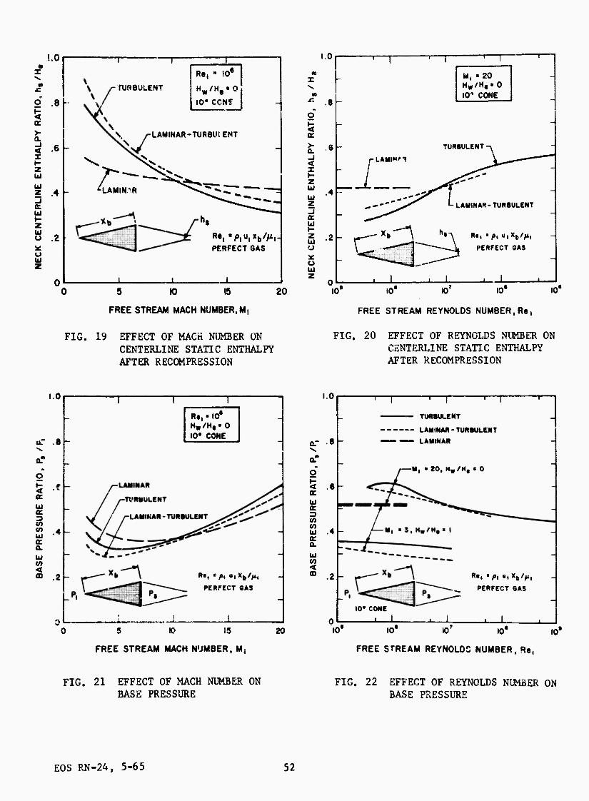
The calculated effects of Mach and Reynolds numbers on the center-

line stagnation enthalpy at recompresolon are shown In Figs. 19 and 20.

The results for h /H as a function of Mach number closely follow those s ä

for the core enthalpy. At high Mach numbers the turbulent results are

far from adlabatlc, and the theory even predicti a decrease In h /H If 7 S e

transition occurs In the mixing layer at Re less than 10 (Fig, 20).

Since the "fast expansion" distortion of the initial profiles has been

neglected In these calculations, h might even be smaller due to this (23)S

effect, If the laminar results carry over to the turbulent case.

Finally, the effect of Mach and Reynolds numbers on the base pressure

Is Indicated In Figs. 21 and 22. Generally speaking, the range of P./Pgo

EOS RN-24, 5-6 5 34

I

I I I

I

is about .3 to .6, regardless of conditions. One notices that at high

Mach numbers the laminar and turbulent predictions appear to agree

within about 15 to. If the theory can be believed under these condi-

tions, then one should not expect transition in the base flow of a

slender re-entry vehicle to be accompanied by a large change in base

pressure. This is in contrast to the situation for Mach 3 adiabatic

conditions (shown in Fig. 22), where a sudden drop in base pressure is

indicated as the flow changes from laminar to turbulent.

EOS RN-24. 5-65 35

1A. CONCLUDING REMARKS

In the present report a new empirical turbulent mixing and bas«

flow model has been constructed which hopefully will be applicable

slender re-entry vehicles. A plausible snethod has been foun^ to extra-

polate turbulent mixing results for low Mach numbers to high Mach number

flows and to include the effects of non-similar and highly cooled turbu-

lent mixing layer development. Reasonable results were found for gross

effects such as the base pressure and rear stagnation enthalpy for a

highly cooled 10 half-angle cone.

The asymptotic mixing layer analysis for adiabatic conditions up to

about Mach 3 can probably be considered reasonable, since the velocity

profile data appear to be correlated. Under these conditions the effect

of any Initial boundary layer thickness becomes negligible, since the

turbulent profiles develop very rapidly. Application of the present

theory to any situation where the initial profile effects may become

important must be considered conjecture at this stage, since no experi-

mental confirmation is presently available. This includes the highly

cooled case at relatively low Mach numbers and all conditions at high

Mach numbers. Hopefully, the p.esent treatment of non-similar turbulent

mixing can serve as a guide to future experiments for these technically

important flow conditions.

EOS RN-24 5-6 5 35

1 I I I

REFERENCES

F.L. Fernandez J.L. Carson D.A. Andersen

"Wake Radar Cross Section of Slender Re-Entry Vehicles," Aerospace Corporation, Rept. BSD-TD- 64-152, Oct. 1964.

2. M.R. Denison E. Baum

"Compressible Free Shear Layer with Finite Initial Thickness/' A1AA Journal 1. 342, Feb. 1963.

3. E. Baum H.H. King M.R. Denison

4. B.L. Reeves L. Lees

"Recent Studies of the Laminar Base-Flow Region," AIAA Journal 2, 1527, Sept. 1964.

"Theory of the Laminar Near Wake of Blunt Bodies in Hypersonic Flow," AIAA Paper No. 6 5-52, Jan. 1965.

W.H. Webb R. Golik L. Lees

"Preliminary Study of the Viscous Inviscid Inter- action in the Laminar Supersonic Near Wake," TRW Space Tech. Labs., Rept. BSD-TDR-64-114, July, 1964.

6. A. Mager "Transformation of the Compressible Turbulent Boundary Layer," Jour, of Aero. Sei. 25, 305, May 1958.

7. O.R. Burggraf "The Compressibility Transformation the Turbulent- Boundary -Layer Equations," Jour. Aero. Sei. 29, 434, April 1962.

8. L. Ting P.A. Libby

"Remarks on Lhe Eddy Viscosity in Compressible Mixing Flows," Jour, of the Aero. Sei. 27, 747, Oct. 1960.

H. Schlichting Boundary Layer Theory, Chapter XXIII, Pergamon Press, New York, 1955.

10. A. Ferri P.A. Libby V. Zakkay

"Theoretical and Experimental Investigation of Supersonic Combustion, Proc. of the 3rd Congress of the International Council of the Aeronautical Sciences, Paper No. 51, Spartan Books, Inc., Wash., D.C., 1964.

EOS RN-24, 5-65 37

11. H.H. King E. Baum

"Enthalpy and Atom Profiles In tue Laminar Separated Shear Layer," Electro-Optical Systems Pes. Note RN-6, March 1%3.

12. D.R. Chapman "A Theoretical Analysis of Heat Transfer in Regions of Separated Flow," NACA TN 3792, Oct. 1956.

13. W.J. Christian "Improved Numerical Solution of the Blaslus Problem with Three-Point Boundary Conditions," Jour, of Aero, Sei. 28, 911, Nov. 1961.

14. R.C. Maydew J.F. Reed

"Turbulent Mixing of Axisymmetric Compressible Jets (In the Half-Jet Region) with Quiescent Air," Sandia Corporation, Res. Kept. SC-4763(RR), March 1963.

15. H.W, Leipmann J. Laufer

"Investigations of Free Turbulent Mixing," NACA TN 1257, Aug. 1947.

16. L.J, Crane "The Laminar and Turbulent Mixing of Jets of Compressible Fluid," Jour. Fluid Mech., 3_, Part I, Oct. 1957.

17. D.E. Coles "The Turbulent Boundary Layer in a Compressible Fluid," Rand Corp., Rept. R-403-PR, 1962.

18. L. Crocco "Transformations of the Compressible Turbulent Boundary Layer with Heat Exchange," AIAA Jour. 1^, 2723, Dec. 1963.

19. C.C. Lin

(editor)

Turbulent Flows and Heat Transfer, Vol. V , High Speed Aerodynamics and Jet Propulsion, Princeton Univ. Press, Princeton, New Jersey, 1959.

I

1

20. D.E. Coles

21. M.W. Rubesin

EOS RN-24, 5-65

"The Law of the Wake in the Turbulent Boundary Layer," Jour. Fluid Mech. _!., Part 2, 191, July 1956.

"An Analytical Estimation of the Effect of Trans- piration Cooling on the Heat-Transfer and Skin- Friction Characteristics of a Compressible, Turbu- lent Boundary Layer," NACA TN 3341, Dec, 1954.

38

I I

22. E. Baum "Ininial Development of the Laminar Separated Shear Layer," AIM Jour. j2i 128, Jan. 1964.

23. E. Baum "Effect of Boundary Layer Distortion at Separa- tion on the Laminar Base Flow," Electro-Optical Systems Res. Note RN-16, Oct. 1963.

24. H.H. King "An Analysis of Base Heat Transfer in Laminar Flow," Electro-Optical Systems Res. Note RiN-14, Sept. 1963.

25. H.H. King "A Tabulation of Base Flow Properties for Cones and Wedges," Electro-Optical Systems Res. Note RN-17, Jan. 1964.

EOS RN-24, 5-65 39

APPENDIX A

Maydew-Reed Dividing Streamline Location

Refentiig to Fig. 2, It may be seen that the total mass flow Inside

the dividing streamline at some station x downstream oi the nozzle exit

must equal the mass flow through the nozzle. Assuming that the flow Is

axisymmetrlc, the mass balance yields

f^DSL

fl p u A e e

L_ _Jexit 2TT pu r drI

—Ix (A-l)

The total mass flov ft through the nozzle was calculared by assuming an

Isentropic expansion from the reservoir conditions tabulated by Maydew

and Reed ' for each run.

Since the e^perlau ntal porfile data u(r) are glvet. by Maydew and

Reed for each station x, the integral of Eq. (A-1) can be evaluated as

a function of l*-s upper limit until Eq. (A-l) Is satistled. This of.

course requires that the density variation be kncvn, anc< this was

assumed to be given by the Crocco integral relation for a perfect gas,

Eq. (18). The dividing streamline velocity is then given by u(r „.),

An estimate of ^he eccuracy of tMs procedure can be obtained by

assuming that the flov Inside the dividing streamline can be arbitrarily

divided into a '.rofile" part and a "potential core" part. If most of

the total ft is In the potential core (as It Is for small x), then a

small error In the value of total ft will have a large effect on the

value of !-incT . Fcr example, at x = 1.5" a 5"7o change in M would pro-

duce about 50 to 100 /o changa In UpCT for tb'i experlnn ntal conditions DSL

but at x = 9" a 5 /o change In ft wovild produce only a 5 /o to l^ fo In

u . The datf. shown in Fig. 3 for x - 1.5 and 3.0 Inches therefore

could le considerably in error.

EOS RN-24, 5-6 5 40

I I I I

APPENDIX B

Eddy Viscosity Factor k of Figure b

When detailed profile data are available, as in the Maydew-Reed

repoit, the factor k in the eddy viscosity expression (Eq. 1) can be

fcund by a least-squares fit of the data with Eq, (19). However, much

of the previous literature on the mixing problem does rot contain

sufficiently detailed profile data, but presents only the final result

in the form of the jet spread parameter a, A summary of previous

experimenial determinations of a up to 196 2 is given by Maydew and Reed,

Since a deper.ds on the choice of profile used in the theory, this must

also be specified.

One way that the quantity k can be related to a is by comparing

the derivatives du*/d(y/x) of Eq. (l?) and (19) at some selected value

of U". For example, for the error function profile

u* = 1/2 (■ - ^ r •-■-] (A-2)

we match the slopes at u* = ,5 to get:

k = /H

\ e/ L

H c

H L. e

/ fl c \

_vCZ.

f - _J TiT .* = .5

(A-3)

1 I 1 I

Thus one must specify the profile shape function g(cy/x) and the

valje of u,v at which the slopes are to be matched.

,iearly the above method for determining k may not be very accurate

and in addition depends on an arbitrary assumption of the value of u*

at which the equr^ion is evaluated. This procedure therefore will not

EOS PN~2A, 5-65 41

be used In this report, with one exception: The data of Zutnwalt at

Mach 3 referred to by Mtydew and Reed provide an additional point on

Fig. 5 which further " ands the correlation.

In a private communication with Prof. Zutnwalt at the University of

Oklahoma it was found for ehe error function profile the best a was

loughly a%23 to 30 at Mach 2.9, depending on how the initial boundary

layer thickness was taken into account. Eq. (A-3) was evaluated at

u* « .5 using this information to give the data points of Fig. 5

attributed to Zutnwalt.

A second point to be made concerns the determination of k by

correlating mixing layer profile data in the non-similar growth region.

This will surely be a problem in high Mach number flows if the relation

of Fig, 5 IJ approximately correct. The mixing layer experiment should

produce either velocity or density profiles (or both) as a function of

physical x and y. The basic equations of this report show that the

theoretical relation for u^Cx^jk) is given implicitely by the relations

y - y 1 \ e au*

DSL J« \ P F' p u r F 4

e e o w U" DSL

F* = F*(S*,u*)

S* = S*(x*, Cf)

C, = Cr ^H /H . h /H , R ) f f w e e e e

x* = \ p u F k r J e e w o Jdx

F = F (C, H /H , h /H , u ) w wfweeew

D = oCP.b)

h = H - u2/2

EOS RN-24, 5-63 42

Thus k appears explicltely in the relation for x* as a function of x,

Although somewhat cumbersome, these relations can be programmced for

a computer so that a least squares deternünation of k from velocity

profile da,a, density profile data, or bat], car In performed.

EOS RN-24, 5-65 43

I

BODY BOUNDARY

LAYER

NONSIMILAR MIXING REGION SIMILAR MIXING REGION

LOW SPEED FLOW (RECIRCULATING CORE)

FIG. 1 MIXING LAYER REGIONS

EDGES OF MIXING LAYER

AXISYMMETRIC NOZZLE H<HC

(AMBIENT CONDITIONS)

FIG. 2 GEOMETRY OF THE JET MIXING EXPERIMENT

3

>- t u o _J LÜ > UJ

1.0 -

i ■6f=-

<J Ui DC h- co

Ü

9 > Q 0

!

JET u/u, föftrm^ ——fc

1 1 1

- U«^"~~B:

, ^ ■ UbL

~*-A

n (-THEORETICAL (CHAPMAN PROflLE)

D

-^- , i ■ i ■„ J J.__.A

- Q

A

A

MACH

O .70 a .ss O 95 |

1

A 149 O 196

PROFILE DATA FROM MAYDEW AND REED

1 1 ! 0 4 6 8

x, INCHES 10 12

FIG. 3

EXPERIMENTAL DIVIDING STREAMLINE VELOCITY CALCULATED FROM MASS BALANCE

EOS RN-24, 5-65 J»4

I ?

u

en Q

O

-I 2

-16

/•CHSIANCE DSl , u"= 58? «''DISTANCE TO VIRTUAL ORIGIN

»■ = SCALING CONSTANT

4 6 8 to VELOCITY RATlO,u/ue

FIG. 4 CORRELATION OF PROFILE DATA

i I I

o t- o 2

o o

o Q

■\ j 1 I , ! ! I

EDDY VISCOSITY €■ .e

MOMENTUM THICKNESS: 9= / u'll-u'l-^-dy

O MAYDEW 8 REED ALEIPMANN ft LAUFER OZUMWALT (ERROR FUNCTION,

o-^3 a 30)

i 1—i—iiit

CORRELATION k = 0606 tr:

100 CROSS-STRFAM DENSITY RATIO />e/^c

EOS RN-24, 5-65 45

FIG. 5

CORRELATION TO DETERMINE THE EDDY VISCOSITY FACTOR k

008

006

2 ÜJ

Ö UJ

004-

002

FIG. 6

EQUIVALENT SKIN FRICTION COEFFICIl'NT

Cr FOR CONES AND WEDGES, H /H = U f we

10* i07 10* 10'

REYNOLDS NUMBER R2 -R« C"»' (jtl) '

iC*

008

006

FIG. 7

EQUIVALENT SKIN FRICTION

COEFFICIENT C FOR CONES

AND WEDGES, H /H = 1 w e

rrm 1—mTTTr

Z ÜJ

> 5 o

004

002

B L TURBULENT AT NOSE

_. i ■ i iiul ' i 11 iiiii i • i < ■■<I-I i i i Mini io- ,0« 10' 10° 10' 10"

.008

IO

z UJ _J

% 5 o UJ

.006-

.004

0U2

I», 2 « Bt-TURBÜLENT ATNOSE

«•RtjCj'd+l)'1

R«2»^, «, «/Mt

^/OWEOGE ' I I CONE

REYNOLDS NUMBER Rj «R.jCV'U + ir

FIG. 8

EFFECT OF WAIL ENTHALPY RATIO

ON C FOR R = I'""7

5 10 15

BOUNDARY LAYER EDGE MACH NUMPER M,

20

FIG. 9

TURBULENT INITIAL HTXING LAYER PROFILE

* u.

"T - T- — -p- ■ ■ T ■ r -,

^LAMINAR SUBLAYER REGION

U- i n * ^^^^

K ^ z: \, UJ ^-ANAirriCAL N < 8 ^ STARTiNG \ SOLUTION K \ /-LAMINAR

V / (BLASIUS) > t 6 C, = 002 004 006 X o o \ -1

\

o 4

UJ f--d*/di

\ \ \ \

-i

1 * - 0

9 V S^ \ o

LA* Of WAUL is. ^^^^^^^ \

_J 1 . _J. . i . t 1

ECS RN-24, 5-65 46 2 A 6 e

VELOCITY RATIO, u/ue

10

X UJ

o

O _l UJ >

z

8 10 .8 l.O

» u.

>- 6-

i i i !s'-io-J|

" /"

\f: \ ^ _/-LAMINAR

\\\ Cf« 002\ 004\ 00fc\

8 10

z Q <

o o

> o UJ

i .2 Z K O z

0

(d1

■ -——I [ r .. p

s#.ttfj

/^:

\

^^^~ LAMINAR

\ \ \ \ \

^■^ Cf ■ ooz >v .004^ v ooeV. \

2 4 6 8 10

I

> 4

4 6 8 iQ

VELOCITY RATIO, U/ü.

10

u. la.

W S < K 0 6 >- H O o _i > * o UJ

< z a:

—r _

f •

I ■ -T i

s». 10

00 o

<!>••/u#(l-u*)^*. Ptu,'0

-00

9 -

LAMINAR

Cf • .002 004 006

__. ^

2 4 6 8

VELOCITY RATIO, u/u.

10

(•) (f)

I FIG. 10 DEVELOPMENT OF THE VELOCITY GRADIENT PROFILES WITH STREAMWISE DISTANCE

EOS RN-24, 5-65 47

■o-7]

ü

(0)

(c)

INiTIAI. BftOFILE

BLASIUS .006

SET OF CURVES FOR S " 10 (FOR S*<löl AU INITIAL PROFILES GIVE SAME CURVE)

2

VELOCITY RATIO, u/u.

1.0

M. H, - (H#-HcUl-y*)-(Hc-Hw)-W

" STUR6•f•wj',•U•K**ro<,',

.6 -

.4 -

S*" I«.

*':f u'U-u*)^ - - * P u r J fl

p

.2 4 6 .8

VELOCITY RATIO, u/u.

1.0

(d)

FIG. 11 DEVELOPMENT OF THE ENTHALPY FUNCTION W PROFILES WITH STREAMWISE DISTANCE

EOS RN-24, 5-65 48

I

I I

I

I I I I t I i E I I

LIMIT 587

^LAM,/r-/>eueMero2i<1*

Fw= ((3uVdY)¥

10 -2 10- 10° 10' in« STREAMWISE DISTANCE PARAMETER, 3*=CF^

FIG, 12 VELOCITY ON THE DIVIDING STREAMLINE

10s

z' g t- u z Zi u. >- a. _i < x Z UJ

UJ

2 < UJ cr

o z 9 > a

Z LIMIT en H = He-(He-HcKI-u*)-(Hc-Hw)W

^LAM^/c^e^Me'o2'0«

k* = 06061-^) funi-u*)^*

Fw = (du*/dY).

STREAMWISE DISTANCE PARAMETER, S*^ Fw

FIC. 13 ENTHALPY FUNCTION W C THE DIVIDING STREAMLINE

EOS RN-24, 5-65 49

10" -.-* ^-1 i0"' 10"' 10" !0

STREAMWISE DISTANCE PARAMETER,S

10'

» 10'

10'

e

UJ

CO (/) ÜJ z ü X

— C^ s .002

10

UJ

o 2

.t_1 rn rn

pi EDDY V:«5C0StT> « = ^ Utö

MOM TKXmESn B -Ju* I - u» ) -^- dy

.004

006

BLASIUS 3TURfl'Fn/^u«LK*1rodx

10" 10 -t

iO" IO" 10

STREAMWISE DISTANCE PARAMETER, S

10' *

IO"

EOS RN-24, 5-65 50

FIG. 14

RELATION BETWEEN x* AND s*

FIG. 15

SMEAR LAYER MOMENTUM THICKNESS INTEGRAL

ENERGY BALANCE CONTROL VOLUME (BOUNOAftt IS (NVISCIO FLO* STREAMLINE 1

DIVIDING STRtAMLINE

BO»« stior

FLOW^

- REAR STAGNATIOM / POINT

BODr BOUNDARY LAYER

<- SEPARATED MIXING LAYEft

RECOMPRESSION ZOHE

FIG. 16

BASE FLOW MODEL

1.0

X

>- a. _i < x t- z UJ

Ld or o ü

2

3 O K ö hi

.4 -

FIG. 17

DIVIDING STREAMLINE VELOCITY BEFORE RECOMPRESSION

-TURBULENT Hw/H,■0 10* CONE

LAMINAR-TURBULENT

3

O 3

<

>

Ö O _l u > UJ z 3 s <

ac

«

z 5 > 5

.2 -

"C R«l s *l «tXb'Ml

PERFECT 6AS

5 W 15

FREE STREAM MACH NUMBER. M,

20

1 \ ' ■ i I "1

\ \ y-TURBULFNT R., •10«

^C N H, 'H, • 0

1 X^ iO' C3NE H

^ ^ *^»^

\ /-LAMINAR-TURBULENT

1 /^^ ■ — ^sx -^

^—LAMINAR ^v^T

^Sd .."^

^|

^<3 «•••^.".V^H PERFECT 6A3

1 5 10 15

FREfT STREAM MACH NUMBER, M.

20

FIG. 18

RECIRCULATING REGION ENTHALPY

EOS RN-24, 5-65 51

1.0 I v.

M

a -i < x t- z UJ

Lü

.6

z .4

UJ o

UJ z

fURBULENT

Re, " 10e

Hw /He»0

10* CONE

LAMINAR-TURBUIEHT

HAMINAR ^SSS,N^r "^ " —'

J. -L

R^-^u,«,,//*, PERFECT GAS

_L

1.0

0 9 10 IS 20

FREE STREAM MACH NUMBER, M,

FIG. 19 EFFECT OF MACH NUMBER ON CENTERLINE STATIC ENTHALPY AFTER RECOMPRESSION

1.0

- .8

< a: UJ oc V) tn UJ a: a. UJ V) < CD

R«, ■ 10* H,/Ht« 0 10* CONE

PERFECT «AS

X 8 10 18

FREE STREAM MACH NUMBER, M,

FIG. 21 EFFECT OF MACH NUMBER ON BASE PRESSURE

20

EOS RN-24, 5-65 52

i

M x:

< (E

>- Q. _l < X H Z UJ

UJ

cc UJ t- z UI

o UJ z

.8 -

.2 -

- . I T ... T. !

'

- M, « 20 H„/H#»0 10" CONE

-

TÜRiULENT -^

-

rLAMI»"? ; ^^—— ' "

" i L LAMINAR-TURBULENT

-

- ^-x^^ —~~A PERFECT 8AS

-

. 1 1 l 1 1 10* 10* 10 10" 10'

FREE STREAM REYNOLDS NUMBER.Re,

FIG. 20 EFFECT OF REYNOLDS NUMBER ON CENTERLINE STATIC ENTHALPY AFTER RECOMPRESSION

i.O

i- < a: UJ (E

(/) W UJ a: a. ui

< ID

TURBULENT

LAMINAR-TURBULENT

— LAMINAR

-M, « 20, H,/Ht < 0

^ PERFECT 6AS

10* CONE

10* 10' I0T lO* 10*

FREE STREAM REYNOLDS NUMBER, Re,

FIG. 22 EFFECT OF REYNOLDS NUMBER ON BASE PRESSURE

I I I I I I I I I I I I I I I I I I