Page 1
RNA Sequence to Structure Mapping
DISSERTATION
zur Erlangung des akademischen GradesDoktor rerum naturalium
Vorgelegt der
Formal- und Naturwissenschaftlichen Fakultatder Alma Mater Rudolphina zu Wien
von
Stephan Kopp
am Institut fur Theoretische Chemie und Strahlenchemie
im September 1998
Page 2
Abstract
Motivated by the observation, that RNA folding gives rise to extended neutralnetworks in sequence space, concepts of random graph theory are applied tobuild a model of RNA sequence to structure mappings. This model allowsto investigate generic properties of sequence-structure relations as well asthe effect of neutrality. The random mapping construction is based on twotunable parameters. These parameters pu and pp resemble the average degreeof neutrality for unpaired and paired part of the RNA secondary structure,respectively. In the model a set of secondary structures must be given.
The mapping is performed by building the preimage of the structures. Forthis purpose, the set of sequences C is constructed which are compatible witha given structure s. From this set, sequences are chosen with a probabilitydetermined by pu and pp, and finally assigned to the structure s, if (and onlyif) this sequence has not been mapped to another structure. The propertieswe are focusing on are the existence of extended neutral nets in sequencespace, the connectivity of these nets and their denseness in C.
The mathematical theory for our model claims the existence of a thresholdvalue for connectivity and denseness properties of neutral nets. The theoremshold in the limit of infinite chain length and determine the threshold valueto be p∗ = 1− κ−1
√
1/κ in both cases. Here, κ is the size of the alphabet usedto encode the unpaired or paired parts of the sequences, respectively. Belowthis threshold the nets are neither connected not dense in C, whereas abovethe threshold almost all nets are connected and dense in C.
Computer experiments indicate that a threshold exists also for finite chainlength, although it is not sharp anymore. However, within the accuracy of thesimulations the threshold value is identical with the theoretically predictedone. Furthermore, it is identical for both properties.
We investigate the influence of the tertiary contacts on generic propertiesof sequence-structure mappings. Instead of trying to predict tertiary struc-tures of sequences we determine the tertiary contacts. Compatible sequencesare then constructed according to an arbitrary base-pairing rule. This modelalso contains a tunable parameter determining the frequency of tertiary con-tacts in a structure. We show that in this model large neutral networksexist for tertiary structures even in the case where the structures contain arelatively high number of tertiary contacts.
Page 3
Zusammenfassung
Die Faltung von RNS Molekulen weist darauf hin, daß ausgedehnte neu-trale Netzwerke im Sequenzraum bestehen. Diese Beobachtung veranlaßteuns, Methoden der Zufallsgraphentheorie zu verwenden, um ein Modell vonRNS-Sequenz-Struktur-Abbildungen zu entwickeln. Mittels dieses Modellsuntersuchen wir generische Eigenschaften der Beziehungen zwischen Sequen-zen und Strukturen sowie die Auswirkung der Neutralitat. Die Durchfuhrungder Zufallsabbildung beruht auf zwei vorzugebenden Parametern. Diese Pa-rameter pu und pp entsprechen jeweils dem mittleren Grad an Neutralitat inden ungepaarten und gepaarten Teilen einer RNS Sekundarstruktur. In un-serem Modell muß eine Menge von Sekundarstrukturen vorgegeben werden.
Wir fuhren die Sequenz-Struktur-Abbildung durch, indem wir die Ur-bilder der Strukturen erzeugen. Dazu wird die Menge C der Sequenzengebildet, die mit der gegebenen Struktur s kompatibel sind. Mit einerWahrscheinlichkeit, die durch pu und pp bestimmt ist, ziehen wir aus dieserMenge Sequenzen und weisen diese nur dann der Struktur s zu, wenn sienicht bereits einer anderen Struktur zugeordnet worden sind. Unser Augen-merk liegt auf folgenden Eigenschaften: die Existenz ausgedehnter neutralerNetze im Sequenzraum, der Zusammenhang der Netze und deren Dichte.
Die mathematische Theorie des Modells sagt voraus, daß ein Schwell-wert fur den Zusammenhang und die Dichte neutraler Netze existiert. DieTheoreme gelten im Limes unendlicher Kettenlange, wobei der Schwellwertin beiden Fallen p∗ = 1− κ−1
√
1/κ ist. Mit κ bezeichnen wir die Große desAlphabets, mit dem wir die ungepaarten bzw. gepaarten Teile kodieren. Un-terhalb des Schwellwerts sind die Netze weder zusammenhangend noch dichtin C, wogegen oberhalb des Schwellwerts fast alle Netze zusammenhangendund dicht in C sind.
Computerexperimente weisen darauf hin, daß ein Schwellwert auch furendliche Kettenlangen existiert, obgleich er nicht mehr scharf ist. Inner-halb der Simulationsgenauigkeit ist dieser Wert identisch mit dem theoretischvorhergesagten und fur beide Eigenschaften gleich groß.
Wir untersuchen den Einfluß tertiarer Kontakte auf generische Eigen-schaften der Sequenz-Struktur-Abbildung. Anstatt zu versuchen, die tertiareStruktur von Sequenzen vorherzusagen, geben wir tertiare Kontakte vor.Die kompatiblen Sequenzen werden gemaß einer willkurlichen Basen-Paar-Regel festgelegt. Dieses Modell beinhaltet ebenfalls einen Parameter, der dieHaufigkeit der Tertiarkontakte in einer Struktur bestimmt. Wir zeigen, daßin diesem Modell große neutrale Netzwerke fur Tertiarstrukturen auch dannexistieren, wenn die Zahl der tertiaren Kontakte verhaltnismaßig hoch ist.
Page 4
Contents
1 Introduction 1
1.1 The RNA Molecule . . . . . . . . . . . . . . . . . . . . . . . . 1
1.2 A Concept of Evolutionary Adaptation . . . . . . . . . . . . . 3
1.3 The Model of RNA Sequence Structure Mapping . . . . . . . . 6
1.4 Organization of this Work . . . . . . . . . . . . . . . . . . . . 9
2 Theory 11
2.1 Graph Theory and RNA Molecules . . . . . . . . . . . . . . . 12
2.2 Secondary Structures . . . . . . . . . . . . . . . . . . . . . . . 15
2.3 A Random Graph Model Applied to RNA . . . . . . . . . . . 19
2.4 Denseness of Random Graphs . . . . . . . . . . . . . . . . . . 21
2.5 Connectivity and Sequence of Components . . . . . . . . . . . 25
2.6 The Implemented Model . . . . . . . . . . . . . . . . . . . . . 26
2.7 Tertiary Structures . . . . . . . . . . . . . . . . . . . . . . . . 27
3 Algorithms 29
3.1 Generating Random Structures . . . . . . . . . . . . . . . . . 29
3.1.1 Secondary Structures . . . . . . . . . . . . . . . . . . . 29
3.1.2 Tertiary Structures . . . . . . . . . . . . . . . . . . . . 31
3.2 Sequence to Structure Mapping . . . . . . . . . . . . . . . . . 33
3.3 Components of a Neutral Net . . . . . . . . . . . . . . . . . . 35
3.4 Degree of Neutrality . . . . . . . . . . . . . . . . . . . . . . . 36
3.5 Neutral Walks . . . . . . . . . . . . . . . . . . . . . . . . . . . 37
3.6 Storaging Large Numbers of Individuals . . . . . . . . . . . . 39
3.6.1 Encoding of Sequences . . . . . . . . . . . . . . . . . . 39
3.6.2 Storing the States of Integers . . . . . . . . . . . . . . 39
4 Computational Results 43
4.1 Parameters for the Random Mapping Procedure . . . . . . . . 43
4.2 Availability of Compatible Sequences . . . . . . . . . . . . . . 47
4.3 Neutrality in Preimages of Random Maps . . . . . . . . . . . 51
4.4 Distribution of Preimages . . . . . . . . . . . . . . . . . . . . 53
Page 5
4.5 Composition of Neutral Nets . . . . . . . . . . . . . . . . . . . 56
4.6 Neutral Walks in Sequence Space . . . . . . . . . . . . . . . . 60
4.7 Mapping of Sequences into Tertiary Structures . . . . . . . . . 67
4.8 Random Mapping and RNA Folding Data . . . . . . . . . . . 70
4.8.1 Distribution of Preimages . . . . . . . . . . . . . . . . 72
4.8.2 Degree of Neutrality . . . . . . . . . . . . . . . . . . . 74
4.8.3 Composition of Neutral Nets . . . . . . . . . . . . . . . 77
4.8.4 New Structures in Boundary of Neutral Nets . . . . . . 80
5 Discussion 82
6 Conclusion and Outlook 88
Appendix A Supplemented Results 91
A.1 Distribution of Preimages . . . . . . . . . . . . . . . . . . . . 91
A.2 Sequence of Components . . . . . . . . . . . . . . . . . . . . . 91
A.3 New Structures in Boundary of a Neutral Walk . . . . . . . . 93
Appendix B Data Structures 94
B.1 Binary Trees . . . . . . . . . . . . . . . . . . . . . . . . . . . . 94
B.2 Balanced Binary Trees: The AVL-Algorithm . . . . . . . . . . 95
References 96
Page 6
List of Figures
1 Illustration of Hypercube . . . . . . . . . . . . . . . . . . . . . 13
2 Representation of Secondary Structures . . . . . . . . . . . . . 18
3 Random Induced Subgraph . . . . . . . . . . . . . . . . . . . 21
4 Denseness of Graphs . . . . . . . . . . . . . . . . . . . . . . . 22
5 Circle Representation of Secondary Structure . . . . . . . . . . 32
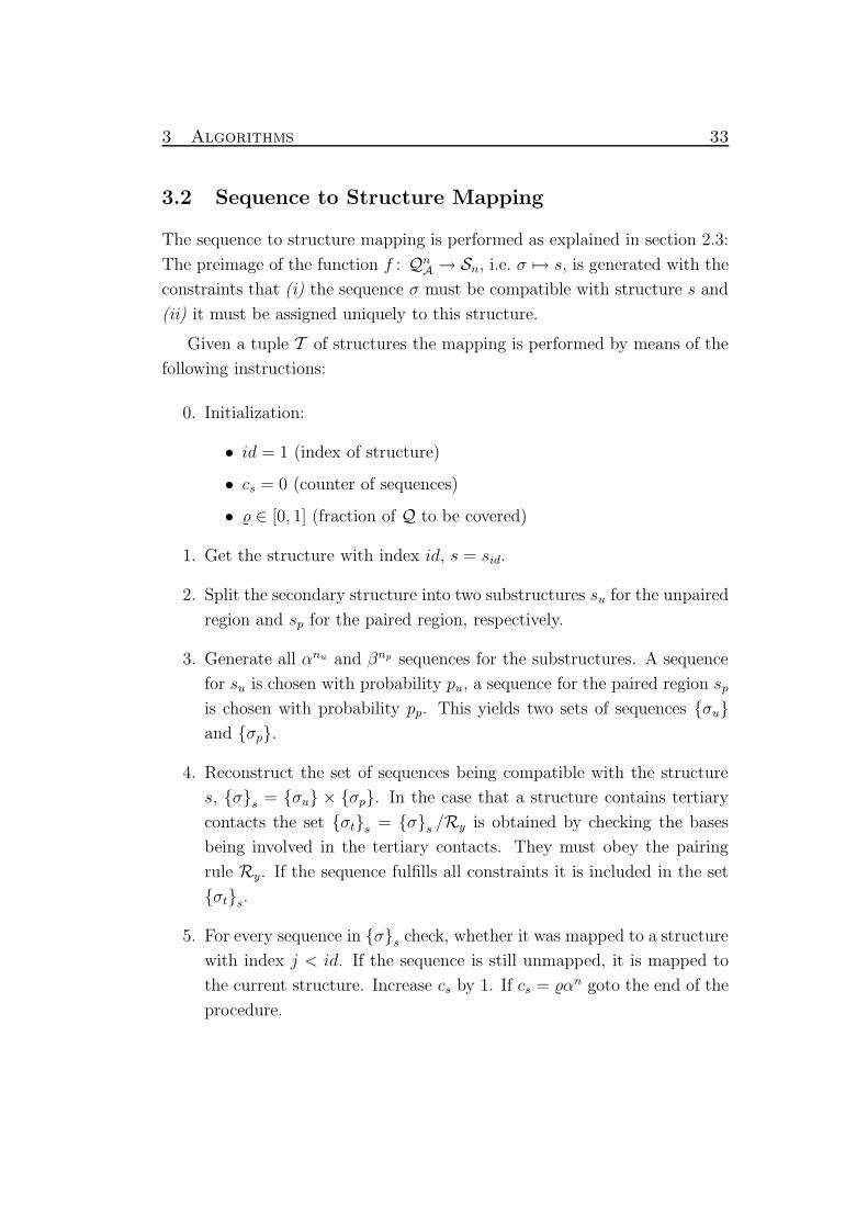
6 Compatible Sequences . . . . . . . . . . . . . . . . . . . . . . 34
7 Increase of Sequences Mapped . . . . . . . . . . . . . . . . . . 40
8 Common mfe Structures . . . . . . . . . . . . . . . . . . . . . 45
9 Network to Compatible Sequences Ratio . . . . . . . . . . . . 49
10 Relative Sizes of the Neutral Nets . . . . . . . . . . . . . . . . 50
11 Degree of Neutrality (unpaired region) . . . . . . . . . . . . . 51
12 Degree of Neutrality (paired region) . . . . . . . . . . . . . . . 52
13 Distribution of Preimages . . . . . . . . . . . . . . . . . . . . 54
14 Fitting Zipf’s Law . . . . . . . . . . . . . . . . . . . . . . . . . 57
15 Number of Components . . . . . . . . . . . . . . . . . . . . . 59
16 Giant Components and Connected Nets of Frequent Structures 60
17 New Structures in Boundary of Neutral Walk . . . . . . . . . 63
18 Number of Sequences in Neutral Walk . . . . . . . . . . . . . 65
19 Covering the Hypercube . . . . . . . . . . . . . . . . . . . . . 66
20 Tertiary Preimage Distribution . . . . . . . . . . . . . . . . . 68
21 Fraction of Compatible Sequences, tertiary structures . . . . . 70
22 Number of Components, tertiary structures . . . . . . . . . . . 71
23 Distribution of mfe structures . . . . . . . . . . . . . . . . . . 73
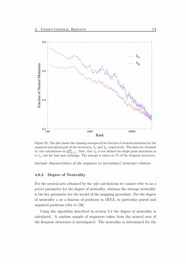
24 Neutrality of mfe preimages . . . . . . . . . . . . . . . . . . . 74
25 Neutrality of Ranks . . . . . . . . . . . . . . . . . . . . . . . . 76
26 Neutral Net Components of mfe Structures . . . . . . . . . . . 79
27 Boundary of Folded Path . . . . . . . . . . . . . . . . . . . . . 80
28 Giant Components and Connected Nets of Rare Structures . . 92
Page 7
iv
List of Tables
1 Common mfe Structures . . . . . . . . . . . . . . . . . . . . . 46
2 Preimages of Mapping Procedures . . . . . . . . . . . . . . . . 55
3 Number of Components . . . . . . . . . . . . . . . . . . . . . 58
4 New Structures in Boundary of Walks . . . . . . . . . . . . . . 61
5 Length of Neutral Walks . . . . . . . . . . . . . . . . . . . . . 64
6 Number of Sequences in Neutral Walk . . . . . . . . . . . . . 64
7 Components of Neutral Nets, Tertiary Structures . . . . . . . 71
8 Degree of Neutrality . . . . . . . . . . . . . . . . . . . . . . . 77
9 Neutral Net Components of mfe Structures . . . . . . . . . . . 78
10 Cover ability of mfe calculations . . . . . . . . . . . . . . . . . 81
11 Fit parameters for Zipf’s law . . . . . . . . . . . . . . . . . . . 91
12 Number of Components for Rare Structures . . . . . . . . . . 92
13 Fitting coefficients for Neutral Walks . . . . . . . . . . . . . . 93
14 Covering Ability of Neutral Walk . . . . . . . . . . . . . . . . 93
Page 8
1 Introduction 1
1 Introduction
1.1 The RNA Molecule
It took almost a century from the first clear evidence of elements of inher-
itance provided by Gregor Mendel’s experiments in the sixties of the last
century [45] to the discovery of the structure of the molecule that carries the
“blueprint” for the phenotype. Although this molecule, the deoxyribonucleic
acid (DNA), was isolated already in 1869 from leucocytes, it was accepted
to be the carrier of the genetic code only in the late forties of our century [2].
An X-ray diffraction photograph taken by Rosalinde Franklin [20] was one of
the most important elements of the puzzle that led James Watson and Fran-
cis Crick to propose a three-dimensional model of the DNA’s double helical
conformation [74, 75]. Its basic simplicity combined with obvious biological
relevance caused immediate acceptance of the model.
The existence of a second kind of nucleic acid, which is located in the
nucleus as well as in the cytoplasm, was already known in the late nineteenth
century. The nucleotides of this ribonucleic acid (RNA) consist of the same
classes of chemical components as DNA: a phosphate group, a pentose and
either a purine or a pyrimidine base [58]. In the 1920s it was found that the
sugar contained in DNA is a deoxyribose, instead of the ribose in RNA. In
both classes of nucleic acids the hetero-cyclic bases, purines or pyrimidines,
are linked together by ribose-phosphate bridges. The purines are adenine
(A) and guanine (G), and the pyrimidines are cytosine (C) and thymine
(T), which is replaced by the base uracil (U) in RNA.
The importance of RNA molecules in viruses and cells is apparent since
RNA serves as messenger (mRNA), carrying the genetic information from
the DNA to the translation apparatus. As transfer RNA, or tRNA for short,
it plays the role of an adapter for the synthesis of proteins. Ribosomal
RNAs (rRNA) function as integral parts of the ribosome and show catalytic
activities in natural polypeptide synthesis (see e.g. [6, 7, 76]). RNA thus was
and is able to serve two purposes: (i) storage of genetic information based on
a one-dimensional template that can be read and copied on request, and (ii)
catalytic properties as ribozymes which require three-dimensional structures
in order to gain efficiency and specificity in processing specific substrates.
Page 9
1 Introduction 2
The discovery of these properties led to a revival of interest in the idea
discussed in the sixties by Francis Crick, Walter Gilbert and Leslie Orgel,
that life was based entirely on RNA before proteins were existent [9, 24, 50].
In this sense the function of an RNA molecule is essentially determined
by its structure. As demonstrated by Sol Spiegelman, in vitro evolution ex-
periments can be applied to selection of RNA molecules that are capable of
fast replication [46]. Indeed, replication rates are optimized in serial transfer
experiments [14, 36, 60]. In case one wants to optimize other properties than
replication, intervention is required making use of special techniques, which
interfere with “natural selection”. A well known example is represented by
the SELEX method – an acronym for “systematic evolution of ligands by
exponential enrichment” – which allows to create molecules with optimal
binding constants [71]. The SELEX procedure is a protocol which isolates
high-affinity nucleic acid ligands for a target, for example a protein, from a
pool of variant sequences. Multiple rounds of replication and selection expo-
nentially enrich the population of species which exhibits the highest affinity,
i.e. which fulfill the required task. This procedure thus allows simultaneous
screening of highly diverse pools of nucleic acid molecules for different func-
tionalities (for a review see, e.g. [13, 40]). Results from those experiments
clearly demonstrate the essential property of RNA molecules, that genotype,
i.e. the RNA sequence, and phenotype, associated to the structure, are com-
bined in one molecule.
At this point, the question arises what is meant by the term structure
of an RNA molecule. One must define the level on which the structures of
molecules are explored. For an X-ray crystallographer a structures is tanta-
mount to a set of atomic coordinates. At a sufficiently high resolution two
structures being formed from different sequences will never be identical. In
order to obtain a more tractable definition that fits better its use in biochem-
istry and molecular biology one needs a coarse grained notation of structures.
One such coarse graining leads to the so-called secondary structure which has
been used successfully during the last three decades. The secondary struc-
ture of an RNA molecule is the list of Watson-Crick (AU and CG) and GU
base pairs. With this definition identical structures can be exhibited by very
different sequences.
Page 10
1 Introduction 3
1.2 A Concept of Evolutionary Adaptation
The results obtained by the evolution experiments mentioned above bring
up the issue of how a given (RNA) molecule of length n can be found among
the 4n possible ones. The formation of RNA structures is regarded as a
mapping from sequence space to a space of all possible structures, called
shape space. The sequence space is the set of all sequences of a given length
where the Hamming distance is used as metric [30]. This metric counts the
number of positions in which two strings of same length differ, or in terms
of RNA sequences, it counts the minimal number of point mutations which
are necessary to transform one sequence into the other. The resulting metric
space is commonly identified with a generalized hypercube(1) , denoted by Q.
The notation of shape space was used previously in theoretical immunol-
ogy for the set of all structures presented by all possible antigens [51, 64].
Several methods, such as tree editing [16, 31, 65], were developed and used
as a metric in shape space, which we denote by S. In general, a mapping f
that relates two metric spaces is a called a combinatory map [19], in this case
f : Q → S. Multiple realizations of such a mapping are well known in mole-
cular biology and biochemistry. One of the first methods was the maximum
matching algorithm [49] which soon was improved to an algorithm which took
into account thermo-dynamical parameters for the formation of secondary
structures [48]. Based on the concept of calculating the structure with min-
imum free energy (mfe) more recent programs were developed [31, 80], but
also other ideas were realized, such as kinetic folding algorithms [28, 47].
In kinetic algorithms stacks are established but can melt again, if other
more favorable structures can be formed. These algorithms do not necessarily
determine the mfe structure, nevertheless the sequence-structure mapping is
unique. The suboptimal folding algorithm (see e.g. [78]) and the partition
function algorithm by John McCaskill [44] present another idea of sequence
structure relation: One sequence can, in principle, form a set of secondary
structures. We will not consider these types of mappings here, but think of
unique and surjective mappings from sequence space to shape space.
(1)An explanation of the generalized hypercube is given in section 2.1.
Page 11
1 Introduction 4
Secondary structures are composed of basic elements such as loops and stacks.
Due to sterical constraints loops contain at least three bases, and stacks of
two or more base pairs are essentially the only stabilizing elements, i.e. iso-
lated base pairs are rare. An upper bound for the number of secondary
structures fulfilling these constraints was derived by Paul Stein and Michael
Waterman [67] and refined in [33]. As a result the shape spaces cardinality
is consistently smaller than that of the sequences space, implying that the
mapping is highly redundant. Computational analysis of a unique mapping
which calculates the mfe secondary structures [63] suggested that searching
for a target structure in sequence space can be considered as an adaptive walk
in a fitness landscape. The notion of fitness landscape was introduced by Se-
wall Wright in the thirties in order to illustrate evolution as an hill-climbing
process on a presumably rugged surface [77].
A landscape is considered a map from a finite, but large set of configu-
rations C into scalar values under a cost or fitness function f : C →. It
also requires a notion of neighbourhood between the configurations, i.e. the
configurations are arranged by a metric. A fitness landscape can be regarded
as a specific case of combinatory maps. Altering a conformation to one which
is found in its neighbourhood usually results in a different fitness value. Thus
an adaptive walk is understood as subsequent mutation of the configuration
in order to find the “fittest” configuration.
Further development of the fitness-landscape idea made this concept to
one of the most powerful for optimization strategies not only in theoreti-
cal biology. It was applied to different fields as, for instance, to spin-glass
models (see e.g. [3]) and to combinatorial optimization problems such as the
traveling salesman problem [42]. The fitness function in these model are the
energy of the spin configurations and the length of the tour, respectively. In
the seventies and eighties the concept of fitness landscapes was applied to
dynamics of evolutionary adaptation [10, 12, 17].
Manfred Eigen initiated an approach towards the principles of early evo-
lution. The development of populations of haploid individuals, represented
by sequences of a given length, such as RNA sequences is described. The
theory is based on the replication and degradation rates and on the copying
Page 12
1 Introduction 5
fidelity q = 1 − p, where p is the mutation rate per nucleotide. An impor-
tant property of the model is the existence of an error threshold p∗ for the
mutation rate. For mutation frequencies above this threshold replication is
nearly random and the sequence information is irrecoverable. Otherwise,
i.e. in case p < p∗, populations form stationary mutant distributions which
are characterized as macromolecular quasi-species. The mutation rate and
the fitness of the various species strongly influence the stationary frequencies
of each species. However, this model does not take phenotypes into consid-
erations, and thus the model is restricted to an explanation of the evolution
of sequence populations. Hence, the question remains unanswered how an
adaptive walk is able to find a solution in the set of structures while the
underlying dynamics takes place in sequence space.
At the present time the mapping from sequence space into fitness values
is simplified by partitioning the task in two steps. First, a combinatory map
(cmap, in the diagram below) realizes the formation of the shape from the
sequence. Subsequently the shape is evaluated by a fitness function f :
sequence spacecmap
=⇒ shape spacefitness
=⇒ scalar value
The restriction of the genotype-phenotype relation to a sequence to struc-
ture mapping allows to study the combined fitness landscape. A computer
model where sequences are mapped to a scalar value according to the di-
agram, allowed to gained insight into evolutionary optimization [17]. This
approach combined replication and mutation, taking place in the space of the
genotype, with selection applied to the phenotype. The concept showed that
the combined fitness landscape inherits its properties from the underlying
sequence-structure relation. Further investigations demonstrated that a very
large number of sequences are mapped to the same secondary structure, and
as a consequence these sequences have the same fitness value [19]. Thus, the
concept of neutrality was derived from studies of RNA sequence-structure
mappings.
The observation of neutrality led to the conjecture of neutral networks
spanning the sequence space [63]. This means, a structure is not only re-
alized by many sequences, but these sequences are even connected through
neutral mutations. Ranking the individual shapes by their frequencies of oc-
Page 13
1 Introduction 6
currence in sequence space yields a distribution obeying a generalized Zipf’s
law [79]. There are a few common structures and many rare ones. The shape
space covering conjecture claims that any random sequence is surrounded
by a ball in sequence space which contains sequences folding into almost all
common structures, although the diameter of this ball is much smaller than
the dimension of the sequence space [16, 61]. This conjecture in combination
with neutral networks is considered an important condition for the success
of selection experiments with RNA molecules as described above.
1.3 The Model of RNA Sequence Structure Mapping
In order to get a better understanding of the relation between RNA mole-
cules and their associated structures a model is used where the context of
sequences and structures is simplified. Based on observations from thermo-
dynamical calculations of secondary structures of RNA molecules, Christian
Reidys applied concepts of random graph theory to build a model of sequence
to structure mappings [53, 54, 56]. An introduction to random graph theory
can be found in, e.g. [4, 15]. This model is suitable to investigate generic
properties of the sequence-structure mappings. The physical-chemical na-
ture of RNA structure formation is not subject of investigation in this thesis.
Results from mfe structure calculations are only used as input parameters
for the computer simulations.
As mentioned above it was found that very large numbers of sequences
are assigned to the same secondary structure [17, 19, 26, 27]. It was also
found, that mutations of sequences which result in the same structure, often
differ in one or two nucleotides only. Investigating an reference sequence
and its structure one can determine the fraction of neutral mutations: the
structures of all mutated sequences are calculated and the mutation is said
to be neutral, if the structures us identical to the reference structure. The
average fraction of neutral neighbours is a parameter which characterizes
important properties of the sequence to structure mapping, called the degree
of neutrality.
In this work, we study a model where the assignment of sequences to
structures does not make use of energy parameters. Instead of trying to de-
Page 14
1 Introduction 7
termine the structure of a certain RNA sequence, the mapping is performed
inversely. This means, that for a given structure the sequences which be-
long to its preimage are determined. Again we point out, that we consider
secondary structures rather than real three-dimensional shapes. As defined
above, the secondary structure is a list of base pairs, which can be represented
by a planar graph without knots or pseudo-knots. Although pseudo-knots
occasionally occur in biological structures, they can be regarded as part of the
tertiary structure, i.e. three-dimensional interactions that occur in addition
to the secondary structure [38, 68].
Beside planar graphs, other equivalent representations for RNA secondary
structures, as for instance rooted ordered trees and paring tables have been
developed [16, 41, 65]. Depending on the context where structures are con-
sidered in, each of these representation has its advantages. Using the rooted
ordered tree representation is particularly suitable to obtain a distance mea-
sure for secondary structures. Planar graphs are the best choice for the
illustration in biological context, while pairing tables are well manageable
for mathematical purposes. In this work, we will make use of a string repre-
sentation also called bracket-dot notation [34], in which unpaired bases are
symbolized by dots and matching pairs of brackets stand for base pairs.
This kind of secondary structure representation is perfectly suitable for
computer handling. We are able to recognize paired and unpaired nucleotides
easily and in combination with the known base pairing rules we are able to
construct sequences, which are compatible with the structure under investi-
gation. A sequence is compatible with a structure if it in principle can form
this structure, i.e. it satisfies the pairing rule. For our intension, this rule
could be arbitrary. Nevertheless, it seems to be reasonable to use a natural
rule which allows the base pairs AU, GC and GU, known as Watson-Crick
and wobble base pair respectively. All the sequences which obey the given
rule, compose the set of compatible sequences, C. We emphasize, that those
sequences fulfill only a necessary condition to be mapped to a structure. At
this point, a sequence is not mapped to a particular structure.
The set C of sequences constitutes the fundamental for the investigation
of the sequence to structure mapping. For all structures being investigated
Page 15
1 Introduction 8
such a set of compatible sequences is generated. An important feature is,
that for any two secondary structure their set of compatible sequences have
a non-empty intersection. This means we will always find at least two se-
quences which are compatible with both structures under consideration. We
make note of the fact, that this is not true for three or more structures.
However, being compatible is a prerequisite for a sequence to be mapped to
a structure but the mapping must be unique. Motivated by the existence of
the degree of neutrality, as found in computer simulations for mfe calcula-
tions [63], a Monte Carlo process is applied to choose sequences from the set
C. The random parameter used in this process determines the probability
for a sequence in C to be finally mapped to one (and only one) structure.
This model of a sequence to structure mapping is used, in order to study
generic properties of the sequence-structure relation, which do not depend on
thermo-dynamical parameters [70]. Therefore, the assignment of sequences
to structures as used in the mfe calculations, or folding for short, is reduced
to a mapping which is based on the degree of neutrality only. We investigate,
whether prominent features of the folding can be identified in our case. The
existence of extended neutral networks is one of these characteristics.
To study the resulting networks of sequences, which belong to the preim-
age of a structure, we will use methods developed in graph theory. The
underlying networks of the structures will be examined for important prop-
erties such as connectivity and accessibility. Freely spoken, connectivity can
be tested in a walk in the network of a structure, where a step is equivalent
to a mutation which conserves the structure. All the sequences which can
be visited in such a walk are said to belong to the same component of the
network. Obviously, a network is connected, if it consists of one component
only.
Consider two different structures, s and s′. The structure s′ is accessible
from the network of the first structure, if a mutation of a sequence belonging
to s, ends in the neutral net of the second structure s′. Instead of investi-
gating the complete network of the structure s, a trial and error approach
is used to perform a neutral walk. Starting from a sequence which belongs
to s, mutations are performed and the resulting sequence is mapped to a
Page 16
1 Introduction 9
structure. Here, an error leads to a new structure, where a success means
that the structure is not altered. It is likely, that many such trials along a
neutral walk will end in the network of a structure which differs from s. This
characteristic, being accessible, is strongly related to the property of networks
to be dense in the set of compatible sequences. The denseness-property of
neutral networks is described precisely in terms of graph theory.
The focus of this study lies on the influence of the a priori probabili-
ties which are used to mimic the degree of neutrality. The set of compatible
sequences C of one structure will never change, but depending on the param-
eter which is used to realize the random mapping, the size of the networks
will vary. Even more interesting is to find an answer how the connectivity and
denseness properties of networks change with different random parameters.
The model which is realized for the sequence to secondary structure map-
ping is extended to a mapping to tertiary structures. The scaffold of those
structures is set up by secondary structures. Additionally, new contacts are
superimposed which are not subjected to any constraints [55]. In this case,
the mapping is based on the assignment of sequences to the underlying sec-
ondary structures. A sequence must then fulfill the base pairing rules for
the tertiary contacts to belong to the neutral net of the structure. It is ob-
vious, that the number of sequences contained in the preimage of a tertiary
structure is smaller than for secondary structure. Nevertheless, unexpected
results are found, when the preimages are investigated.
1.4 Organization of this Work
This work addresses the fundamental questions of genotype-phenotype map-
ping as seen from a mathematical point of view. Sequences which are com-
patible with a given secondary structure are randomly and uniquely mapped
to a structure. The sequences being mapped to a structure set up the neu-
tral network of this structure. Important properties, such as connectivity
and denseness, are immanent to those neutral networks. These characteris-
tics are essential for the understanding of optimization processes on rugged
landscapes. The influence of the random parameters used for different map-
Page 17
1 Introduction 10
pings on these properties is theoretically derived and investigated by means
of computer simulations.
The following chapter will give an introduction to the mathematical tools.
Definitions of sequence space and secondary structures are expressed in terms
of graph theory. Using the terminology of this theory, neutral networks
and their properties are explained. Important theoretical propositions are
presented which are concerned with connectivity and denseness of the neutral
networks. The model of mapping is extended to structures where tertiary
contacts are included.
In chapter 3 the algorithms being used to perform the simulations are
described. The mapping of entire sequence spaces, as they are used in the
simulations of this thesis, requires a fast management of a large amount
of data, which is a non-trivial task even for present day computers. For
example, the state of all sequences, whether they are mapped yet or not
must be traced. An algorithm which allows such a tracing is introduced in
this section.
Results obtained by computer simulations are described and illustrated
in chapter 4. We will see, that the number of tertiary contacts has a sur-
prising impact on the composition of the neutral networks. A discussion
follows in chapter 5 and this work closes with chapter 6 where the results are
summarized and an outlook for further investigations is presented.
Page 18
2 Theory 11
2 Theory
RNA molecules are predestinated for studies of evolution in vitro and in
silico, because they combine the genotype and phenotype in one molecule
and because their secondary structures can be determined quite fast. To
this end, a mathematical model handling RNA sequences, their secondary
structures and dynamics in sequence space is required. Such a model has
been derived by concepts from graph theory. In this thesis the focus lies on
the relation of the genotypes belonging to the same phenotype. Therefore,
the brief sketch of graph theory mainly concerned with the sequence space.
In the case of RNA sequences and their secondary structures a common
method to realize such a mapping is to use various algorithm which calcu-
late a secondary structure of any given sequence [28, 31, 43, 44, 80]. The
algorithms make use of thermo-dynamical parameters which have been de-
termined experimentally for several structural elements [21, 52, 72]. Still, the
methods of structure calculation vary and therefore the secondary structure
predicted by these programs are quite different for the same sequence.
Although these folding algorithms do not calculate identical structures
given the same sequence it was found, that the mapping inherit some ba-
sic features which are common to all algorithms [69, 70]. For example, the
distribution of the structures is highly non-uniform: It follows a general-
ized Zipf’s law, i.e. there are few structures which are realized by most of
the sequences, whereas most of the structures have a few sequences being
mapped to them [79]. Another intrinsic characteristic of these mappings is
the existence of neutral networks.
The average fraction of neutral neighbours is the link which allows us to
relate random graph theory of neutral networks and combinatory maps as
they are obtained by folding RNA sequences into secondary structures. The
model, as developed by Reidys, distinguishes between fractions of neutral
neighbours derived from single base mutations in unpaired regions and those
fractions derived from base pair mutations in double helical regions. The in-
vestigation of these networks exhibits additional, interesting properties such
as connectivity and denseness. In order to describe these terms precisely
Page 19
2 Theory 12
the following sections provide the theoretical background. The model, as
developed by Reidys, is presented which is used to simulate the sequence to
structure mapping [56].
2.1 Graph Theory and RNA Molecules
The basic objects of graph theory are vertices and edges. The vertices are
elements of a set, for instance n-tuples of integers in n or strings which are
composed of n elements of an alphabet consisting of κ letters. Here, n is
a finite natural number. In the former case one obtains an infinite graph,
whereas in the latter the graph is finite, if κ is finite. Edges are connections
between pairs of vertices.
In general, the size of an alphabet is denoted by κ. In this work, we will
deal with two distinct alphabets A and B. We will refer to their sizes by α
and β, respectively. The alphabets will be described in this section and in
section 2.2.
In the case of natural RNA molecules we deal with a finite alphabet which
consists of four letters A = A, C, G, U, corresponding to the bases adenine,
cytosine, guanine and uracil (see section 1.1). The nucleotides containing
these bases are linked together by ribose-phosphate bridges (backbone) to
form the sequence or primary structure. As a result, this single strand is
directional and starts with a phosphate unit at the 5′-end and terminates
with a ribose unit at the 3′-end.
In order to apply graph theory, RNA molecules are considered as se-
quences or strings over A, denoted by σ. Such a string corresponds to a
vertex. Due to the fact, that the two ends of an RNA sequence are chemi-
cally different there exist no palindromes in strict sense and the nucleotides
of a molecule can be numbered uniquely, starting at the 5′-end.
In the set of all sequences of constant length n, we add, for example, edges
by connecting vertices which differ in exactly one position, i.e. when their
Hamming distance is one [30]. An edge is equivalent to a point mutation of a
sequence. The resulting graph is called (generalized) hypercube of dimension
n [11]. An illustration of two hypercubes based on the natural four letter
Page 20
2 Theory 13
(A)
A
C G
U
(B)
GG
AG
UGUC
GC CC
UU
UA
CG
AC
AU
GU
CA GA
AA
CU
Figure 1: The hypercube based on a four letter alphabet A = A,C,G,U. The edges
connect two vertices which differ in exactly one position. (A) Hypercube of dimension n=1,
i.e. the length of the vertices is one. The hypercube is regarded as regular tetrahedron.
(B) Hypercube of dimension n=2. It is obtained by quadruplication of the hypercube of
dimension one. The black edges show point mutations in the first position of the vertex.
The colored connections represent mutations in the second position yielding a tetrahedron
with slightly distorted edges for the sake of clarity. Generally, the hypercube of dimension
n+1 is obtained by quadruplicating the hypercube of dimension n.
alphabet for RNA is given in figure 1. Starting with a hypercube of dimension
n=1, as shown in part (A) of this figure, the hypercube of dimension n+1
is obtained by quadruplication of the existing one. One of the four letters
is appended systematically to each vertex. Iteration of this procedure leads
to conceptually simple objects which, however, are too sophisticated to be
drawn on paper.
By mere inspection, one finds some basic properties which are intrinsic
for generalized hypercubes: a) The maximal distance between two sequences
σ and σ′ of the hypercube is dH(σ, σ′) = n, independently of the size of
Page 21
2 Theory 14
the alphabet. b) Every vertex has exactly n · (κ − 1) neighbours accord-
ing to the number of different single point mutations of an RNA sequence.
We will formulate these observations in terms of the following notation and
definitions.
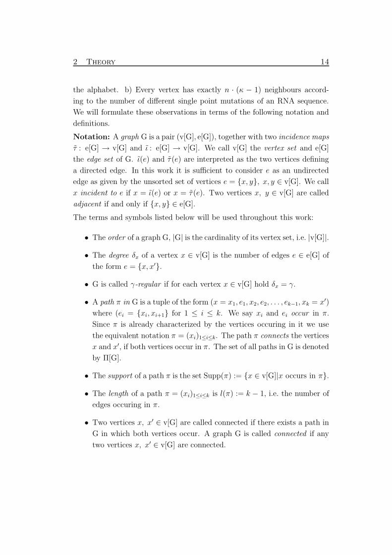
Notation: A graph G is a pair (v[G], e[G]), together with two incidence maps
τ : e[G] → v[G] and ι : e[G] → v[G]. We call v[G] the vertex set and e[G]
the edge set of G. ι(e) and τ (e) are interpreted as the two vertices defining
a directed edge. In this work it is sufficient to consider e as an undirected
edge as given by the unsorted set of vertices e = x, y, x, y ∈ v[G]. We call
x incident to e if x = ι(e) or x = τ (e). Two vertices x, y ∈ v[G] are called
adjacent if and only if x, y ∈ e[G].
The terms and symbols listed below will be used throughout this work:
• The order of a graph G, |G| is the cardinality of its vertex set, i.e. |v[G]|.
• The degree δx of a vertex x ∈ v[G] is the number of edges e ∈ e[G] of
the form e = x, x′.
• G is called γ-regular if for each vertex x ∈ v[G] hold δx = γ.
• A path π in G is a tuple of the form (x = x1, e1, x2, e2, . . . , ek−1, xk = x′)
where (ei = xi, xi+1 for 1 ≤ i ≤ k. We say xi and ei occur in π.
Since π is already characterized by the vertices occuring in it we use
the equivalent notation π = (xi)1≤i≤k. The path π connects the vertices
x and x′, if both vertices occur in π. The set of all paths in G is denoted
by Π[G].
• The support of a path π is the set Supp(π) := x ∈ v[G]|x occurs in π.
• The length of a path π = (xi)1≤i≤k is l(π) := k − 1, i.e. the number of
edges occuring in π.
• Two vertices x, x′ ∈ v[G] are called connected if there exists a path in
G in which both vertices occur. A graph G is called connected if any
two vertices x, x′ ∈ v[G] are connected.
Page 22
2 Theory 15
• The distance dG(x, x′) of vertices in G is the minimum length of all
paths connecting x and x′. If there exists no path connecting the two
vertices we set dG(x, x′) = ∞. The index G is omitted, if no confusion
is possible.
• The boundary ∂GV in G of a set V ⊂ v[G] is
∂GV := x′ ∈ v[G] \ V| ∃ x ∈ V : dG(x, x′) = 1.
The closure in G of V ⊂ v[G], V, is given by V := V ∪ ∂GV.
Note: The index G is not used, if no confusion can arise.
• G′ is a subgraph of G, G′ < G, if v[G′] ⊂ v[G] and e[G′] ⊂ e[G].
• Let H ⊂ v[G]. The induced subgraph or spanned subgraph of H in G,
G[H], has the vertex set v[G[H]] = H. The edge set e[G[H]] is the
subset of all edges in e[G] where both incident vertices belong to H.
• The ball centered at x ∈ v[G] with radius r is the set
Br(x) := x′ ∈ v[G] | d(x, x′) = r.
We summarize that the sequence space is represented as generalized hyper-
cube Qnκ, or just Q, if no confusion can arise. The set of sequences are the
vertices of the hypercube, i.e. v[Q] = σ1, σ2, . . . , σκn. Two vertices σ and
σ′ are connected by an edge e ∈ e[Q], where e[Q] is the set of all edges in Q
whose vertices have Hamming distance one: dH(σ, σ′) = 1. The generalized
hypercube Qnκ forms an undirected graph with the defined vertices and edges.
Every vertex has out-degree (κ − 1)n. An edge e with origin o(e) = σ and
terminus t(e) = σ′ is interpreted as a point mutation leading from σ to σ′
and vice versa.
2.2 Secondary Structures
The secondary structure of an RNA molecule is a list of base pairs. A base
pair is a complex formed by intramolcular hydrogen bonds between a purine
Page 23
2 Theory 16
and a pyrimidine base. The bases can be considered as “sidechains” in the
case of RNA [66].
Secondary structures are also described by means of graph theory. A
mathematically correct and sufficient way for our purposes is to translate
the list of base pairs into an adjacency-matrix Aij [63]. Contacts defined as
tertiary interactions are not included in this definition. The n × n matrix
fulfills the following conditions:
1. aij = 1 for 1 ≤ i ≤ n and j = i± 1 (backbone).
2. For each i there is at most one j 6= i± 1 such that aij = 1 (base pair).
3. For any j 6= i± 1 and l 6= k ± 1 it holds: If aij = 1 and akl = 1 than it
is i < k < j ⇒ i < l < j and vice versa (knot-free).
This matrix can easily be translated into a planar graph, consisting of n
vertices: s = (x1, . . . , xn) . In contrast to the previous definition (section 2.1),
here, a vertex is a single nucleotide. Edges exist only between those vertices
which form a base pair, i.e. if the corresponding coefficient aij is not zero.
We further state, that each of the n vertices has an out-degree δ ≤ 3. This
means a vertex x may have at most one non-backbone bond. Base pairs,
i.e. non-backbone bonds, are also referred to by the term contact.
From the adjacency matrix we derive the set of contacts for a structure
s: Π(s) := [i, j] | aij = 1, i, j = 1, . . . , n, |i − j| 6= 1. The bases being
involved in a contact are called paired, the other bases are called unpaired.
The number of unpaired bases is denoted by nu(s), the number of base-pairs
by np(s), i.e. n = nu(s) + 2np(s). Usually, the argument s is omitted. If a
structure contains no bases pairs, i.e. Π(s) = ∅ the structure is called open
structure.
Let [i, j] ∈ Π(s) be a base pair and let all bases i+1, . . . , j−1 be unpaired.
These bases form a loop closed by the pair [i, j]. Due to steric constraints the
number of unpaired bases in a loop, L, is at least 3. Rule (2) from above can
be generalized, so that for each i, there is at most one j 6= i±L, with L ≥ 3
such that aij = 1.
Page 24
2 Theory 17
Beside planar graphs, various representations of secondary structures have
been developed [41, 65]. Examples of secondary structure representations are
given in figure 2. The adjacency matrix is shown in part (A). The bullets
indicate the backbone and base pairs. A translation into a planar graph is
presented in part (B) of this figure. Biologist use to label the vertices with the
one letter code of the bases which occur at the corresponding position in the
sequence. The string notation, also denoted by dot-bracket notation [34], is
shown in part (C). The string notation represents a secondary structure by a
string of length n: ‘s1 . . . sn’. An unpaired vertex k is denoted by a single dot
sk=‘.’ and pair [i, j] with i < j is represented by si=‘(’ and sj=’)’. Condition
(3) from above renders intercalating parenthesis, e.g.( ( ( ) ) ) , illegal
and thus the assignement of such a string to a secondary structure is unique.
In this work, we will make use of the string notation, since unpaired and
paired regions of the structure can be determined in a straightforward way.
Which representation is used, depends strongly on the context where
structures are considered in. For instance, rooted ordered trees (figure 2(D))
are suitable to determine a distance between secondary structures [16, 19].
In this image, base pairs are mapped into internal nodes , unpaired residues
to leaves, starting at a root (node) which has not correspondence in the
molecule. The root prevents to get lost in a forest of trees. An alteration of
the structure is equivalent to a move of nodes and leaves in the tree. These
moves are associated to certain amount of ‘costs’, and thus the total cost
which is needed to transform one tree into another gives the distance.
From biophysical chemistry we learn, that helical regions of RNA struc-
tures are made of distinct base pairs, which are energetically prefered, for
instance AU and GC pairs. This yields a pairing rule of nucleotides. The
rule can be expressed as an alphabet B coding for the paired positions. The
symbols in this alphabet consist of two letters taken from the alphabet A,
i.e. B ⊂ A × A. Therefore, we define the notion of compatibility between
sequences and structures:
Notation: A sequence σ is compatible with a structure s if and only if for all
base pairs [i, j] ∈ Π(s) the corresponding bases i and j are elements in B. The
set of sequences being compatible with a structure s, or set of compatibles for
Page 25
2 Theory 18
155
10
15
10
5
3’5’
5’
15105
...((((...))..))..3’
5
5
10
15
15
10
(A)
(B)
(C)
(D)
Figure 2: Four equivalent representations of an RNA secondary structure. (A) The list
of base pairs is translated into a adjacency matrix. The numbers show the position of
the nucleotides. Black dots correspond to base pairs where the gray dots represent the
backbone. Due to its symmetry, the matrix can be reduced to a triangle representation.
(B) The same secondary structure drawn as a planar graph. The backbone is shown as
gray line, the base pairs by black lines. (C) The string representation of this structure.
Since the structure is knot-free, matching parentheses stand for base pairs. (D) Tree
representation: base pairs correspond to nodes (black circles), unpaired bases correspond
to leaves. See also text for details.
short, is denoted by C[s]. If the structure is not the open structure v[C[s]]
is a true subset of v[Q] containing αnu · βnp vertices, where β = |B|.
Natural RNA molecules exhibit base pairs, which can be represented by
the alphabet B = (AU), (CG), (GC), (GU), (UA), (UG). With respect to
the chemically different ends of RNA sequences we distinguish between a
(AU) and a (UA) pair, for example. The grouping of the nucleotides stresses
the notation of the base pairs as symbols in B. The set of compatibles
for a given structure s can therefore be determined exactly. An important
observation is, that the set of compatible sequences of two different structures
C[s] and C[s′] always have a nonempty intersection. A prove of this claim
can be found in, e.g., [54]. An example how those compatible sequences are
generated is given in figure 6 on page 34. We will come to this when the
Page 26
2 Theory 19
algorithm of the sequence to structure mapping is presented in detail. We
remark, that the generalization of this statement to three and more structures
is not valid.
We make note of the fact, that the set C[s] again forms a graph. The
sequences in this graph are connected by edges which are considered as com-
patible mutations. This means, that those positions where the nucleotides
are unpaired, single point mutations are performed. At the paired position
the mutations is regarded as an exchange of one symbol of the alphabet B,
which usually is an exchange of two letters from A.
2.3 A Random Graph Model Applied to RNA
The mathematics presented in this section is applied to model sequence-
structure relations, which are based on random graph theory [4, 15]. This
relation is regarded as a mapping [54, 56]. In general, a mapping is a triple
(f, A, B), where elements of the set A are mapped to elements of the set
B according to the (mapping) function f . Here, the set A is formed by
sequences of a fixed length n. The set of all secondary structures which can
be formed by sequences of given chain length constitutes the set B, also called
shape space as it was previously defined in theoretical immunology [51, 64].
We will denote the shape space by S.
To study generic properties of the sequence-structure relations a model
is proposed which does not make use of physical and chemical parameters.
Before we describe the details of the model, a brief sketch is given. There are
two major steps setting up the procedure of the random mapping: Firstly, a
set of possible secondary structures is constructed, i.e. the set B in the map-
ping is generated. Secondly, sequences are assigned uniquely to the structures
setting up the preimage of the structure. This assignment is the elementary
process of the random mapping: sequences compatible with the structure are
generated and accepted with a probability p which is determined in advance.
The algorithm which realizes this mapping is presented in section 3.2.
The model of sequence to structure mapping is mainly based on random
maps. For the convenience of the reader we recall the basic terminology of
probability theory, which is used to describe the propositions and theorems
Page 27
2 Theory 20
of the model. The random map and the properties which are derived from
mathematical considerations are presented next.
Notation: The set Ω is assumed to be finite. This yields a probability space
(Ω,P(Ω),µµµ) which is a triple consisting of the point set Ω, the power set P(Ω)
of Ω and a probability measure µµµ. The measure of an arbitrary set S ∈ P(Ω)
is simply given by summing the point measures: µµµS =∑
ω∈S µµµω.
A random variable X is a µµµ-measurable function X : Ω →. The
distribution of the random variable X is determined by the (cumulative)
distribution function F (x) =µµµX < x, where −∞< x <∞. In the case of
integer-valued random variables we can specify them as well as the probability
density function f(x)=µµµX =x .
The expectation value of a random variable X is defined as the weighted
sum over all points ω ∈ Ω: E[X] =∑
ω∈Ω ωµµµω. The variance of the
random variable is given by V[X] = E[(X −E[X])2].
The idea of the random mapping is freely described as follows. A graph
H, i.e. the vertex set v[H] and the edge set e[H], are given. By choosing
some of the vertices at random with a probability 0 ≤ p ≤ 1, a subgraph
G=H[X] is induced. The edges of G are only those which also occur in H,
meaning that no new edges can be generated. The draft of a random induced
subgraph is illustrated in figure 3. The probability measure of such a graph is
determined by the number of vertices it contains. The mathematical precise
definition of a random graph is given in the following lines:
Model of Random Map: Let H be a finite graph. The each subset of the
vertex set of this graph, X ⊂ v[H], induces the subgraph H[X]. The set of
all induced subgraphs of H is denoted by G(H). A parameter p ∈ [0, 1] is
given and for every graph Γ ∈ G(H) we set
µµµpΓ = p|v[Γ]|(1− p)|v[H]|−|v[Γ]|.
Since this is the probability of a binomial distribution it is clear that
∑
Γ∈G
µµµpΓ = 1.
Hereby we obtain a probability space (G(H),P(G(H)),µµµp).
Page 28
2 Theory 21
H X⊂v[H] G=H[X]
Figure 3: The diagrams show a graph H and one induced subgraph G. Left: The parent
graph H is presented. Middle: A random processes is performed to choose vertices defining
the vertex set X⊂v[H ] of the subgraph. Right: Only the edges which occur in the parent
graph are existent in the induced graph G.
We apply this definition to the model of random sequence to structure
mapping. The parent graph is identified with the set of compatible sequences
of a secondary structure as explained in section 2.2. The vertices are chosen
with probability p resulting in the preimage of the secondary structure. We
denote this preimage by Γ[s], i.e. the random graph of sequences which are
randomly mapped to the structure s, due to the mapping f . In this sense,
the original mapping f : Q → S is inverted and we write
Γ[s] = f−1(s) ⊂ C[s] \⋃
s′∈Ss′ 6=s
(Γ[s′] ∩C[s]) (2.1)
where f is identified with the random choice of sequences. For all secondary
structures in S, the associated preimage is generated by randomly choosing
the sequences from the set of compatibible sequences C.
2.4 Denseness of Random Graphs
The following theorem and its proof were proposed by Reidys [54]. The
theorem is based on a family of configuration spaces (C)n. For our intentions
it is sufficient to identify a configuration space with the generalized hypercube
Page 29
2 Theory 22
G, ∂G H F , ∂F
Figure 4: Illustration of the term denseness. Two subgraphs G and F of a (parent)
graph H are shown on the left and on the right hand side of H , respectively. The vertices
belonging to the subgraphs are shown as black colored circles. The boundary of the graphs
∂G and ∂F are displayed as gray circles. In the case of the subgraph G the vertex set of
the closure, i.e. v[G ∪ ∂G] is identical with H , hence G is dense in H . This not the case
for the subgraph F .
as introduced in section 2.1. A sequence of configuration spaces is obtained
by increasing the dimension of the hypercube, i.e. the length of the sequences
increases. The principle, how such a family is obtained is shown in figure 1.
Here, we will introduce the theorem and its predication. A sketch of the
proof and its implication for the model discussed in this work is given. The
complete proof is found in [54]. Let us begin with the definition of the
relevant terms.
Definition 2.1: Let H be a finite graph. A subgraph G < H is called dense
in H if and only if v[G] = v[H].
The meaning of dense is illustrated best in a diagram. In figure 4 a graph
H is shown in the middle part of the figure. Two subgraphs G and F are
displayed on the left and right side of H, respectively. The vertices of these
graphs are shown as black colored circles. The according boundaries ∂G and
∂F and are displayed as gray circles. In this figures G is dense in H, since
the vertices of closure of v[G] are identical with v[H]. The subgraph F is not
dense.
Page 30
2 Theory 23
The denseness property of random graphs Γ<C are discussed in this section.
To this end, we introduce a random variable
Z(Γ) := |v ∈ v[C]|v 6∈ v[Γ]|
which counts the number of vertices in the configuration space having no
adjacent vertex in the graph Γ.
The measure µ is motivated by looking at a vertex v and its degree γ.
This results in a measure which takes into account the number of edges and
hence the vertices being adjacent to v. The measure is written as:
µ := limn−>∞
(|Cn|(1− p)γn+1)
In the case that p=0 we find µ→∞, where µ=0, if p=1. For a probability
0 < p < 1, the value of µ may also diverge. In the case that µ is finite, one
proves that the distribution of the random variable Z converges to a Poisson
distributed random variable, i.e.
lim→∞
µµµZ = l =µl
l!e−µ.
For an infinite µ we find that lim →∞ µµµZ ≥ l=1 for all l ∈
. This means,
that the number of vertices which are not adjacent to the graph Γ tend to
become infinite.
Equipped with this information we can state the theorem that, under a
certain condition, a random graph is dense in the configuration space.
Theorem 2.1 Let (Cn)n be a family of configuration spaces such that p∗ :=
limn→∞(1 − |Cn|−1/γn) exists and 0 < p∗ < 1. Let Gamman < Cn be an
induced subgraph. For p > p∗ holds:
limn→∞
µµµnΓn is dense in Cn = 1
and for p < p∗ it is:
limn→∞
µµµnΓn is dense in Cn = 0
Page 31
2 Theory 24
In the terminology of random graph theory p∗ is called threshold value for
the denseness property.
The proof mainly relies on the insight gained above. For the Poisson
distributed random variable Z it always holds E[Z] = µ, and here we have
E[Z] = |Cn|(1− p)γn+1. Determining the limits for the expectation value we
find
lim→∞
E[Z] =
0 for p > p∗
∞ for p < p∗
and with the discussion of the random variable Z from above we derive µ=0
and hereby µµµZn =0 = 1, because the variable Z is Poisson distributed(2).
Therefore, we see that µµµZn = l = 0 for any l > 0. This means that in
the limit of infinite length n we expect that there is no vertex, which is not
adjacent to Γ. Hence Γ is dense in C.
For parameter p < p∗ we derive the opposite, because µ → ∞ and thus
µµµZn≥ l = 1: almost no vertex is adjacent to the graph Γ.
Applying this results to the hypercube QnA, which is equivalent to a se-
quence space, we have γn =n(α− 1). With |Cn|= |QnA|=αn we calculate the
threshold value
p∗ = 1− α−1√
1/α.
We summarize this section with the statement, that for a random pa-
rameter p > p∗ almost every random graph Γn is dense in Cn and almost no
Γn is dense in Cn for p < p∗. Using the random mapping as described in
equation (2.1) we expect, that the sequences which are mapped to a struc-
ture yielding in Γ[s] are dense in the set of compatible sequences C[s]. In
combination with the fact that for two secondary structures s and s′ their
set of compatibles have a nonempty intersection, we will study how a virtual
optimization process is realized.
(2)For a Poisson distributed random variable with parameter µ holds: all moments of
the distribution are µ. Further, a distribution is known if all its moments are known.
Page 32
2 Theory 25
2.5 Connectivity and Sequence of Components
Although the term connectivity is clear by intuition, we will recall some def-
initions: Two vertices v and v′ of the set v[G] are connected if there exists
a path in G which contains both vertices. The graph G is connected if
for all pairs of vertices v, v′ ∈ v[G] a path exists in G where both vertices
occur. Otherwise the graph is disconnected. All the vertices which are con-
nected build a subset V of v[G]. A component of G is an induced subgraph
G′ = G[V ] of a maximal connected subset of vertices. We neglect the trivial
components which are induced by the empty set, i.e. G[∅]. In the case that
G is disconnected we will investigate the sequence of components, i.e. a list
of the maximal connected subgraphs of G into which G can be decomposed.
For an illustration we refer to figure 4 (page 21). The graph F consists
of one component, whereas G on the left hand side is decomposed into four
components, one of size 16 and three of size one. From this figure one derives
the definition:
Definition 2.2: Given a graph G, the sequence of components of G is the
ordered tuple (|χi|) with 1≤ i≤ |G|. Each χi is a component of G and we
order these components according to |χi| ≥ |χi+1|. A component is called
giant component if and only if |χ| ≥ 2/3|G|.
A component of size one is called isolated vertex, or in terms of graph
theory, it is a vertex with the property ∂v ∪ v[Γ] = ∅.
In the following we assume that the limes limn→∞(1−|Cn|−1/γn) exists and
fulfills 0< lim(1− |Cn|−1/γn)<1. Further we set p∗ := limn→∞(1− |Cn|
−1/γn).
Before the theorem of connectivity can be formulated, we will discuss
some claims and propositions. For a parameter p<p∗ and for l ∈
one can
prove
limn→∞
µµµΓn contains at least l components with |χ| ≤ γn
which finally yields in the observation
∀l ∈
: limn→∞
µµµΓn has more than l isolated vertices = 1.
Page 33
2 Theory 26
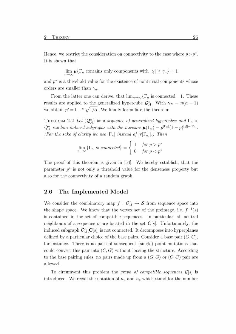
Hence, we restrict the consideration on connectivity to the case where p>p∗.
It is shown that
limn→∞
µµµΓn contains only components with |χ| ≥ γn = 1
and p∗ is a threshold value for the existence of nontrivial components whose
orders are smaller than γn.
From the latter one can derive, that limn→∞Γn is connected=1. These
results are applied to the generalized hypercube QnA. With γN = n(α − 1)
we obtain p∗=1− α−1√
1/α. We finally formulate the theorem:
Theorem 2.2 Let (QnA) be a sequence of generalized hypercubes and Γn <
QnA random induced subgraphs with the measure µµµ(Γn) = p|Γn|(1− p)|Q|−|Γn|.
(For the sake of clarity we use |Γn| instead of |v[Γn]|.) Then
limn→∞
Γn is connected =
1 for p > p∗
0 for p < p∗
The proof of this theorem is given in [54]. We hereby establish, that the
parameter p∗ is not only a threshold value for the denseness property but
also for the connectivity of a random graph.
2.6 The Implemented Model
We consider the combinatory map f : QnA → S from sequence space into
the shape space. We know that the vertex set of the preimage, i.e. f−1(s)
is contained in the set of compatible sequences. In particular, all neutral
neighbours of a sequence σ are located in the set C[s]. Unfortunately, the
induced subgraph QnA[C[s]] is not connected. It decomposes into hyperplanes
defined by a particular choice of the base pairs. Consider a base pair (G, C),
for instance. There is no path of subsequent (single) point mutations that
could convert this pair into (C, G) without loosing the structure. According
to the base pairing rules, no pairs made up from a (G, G) or (C, C) pair are
allowed.
To circumvent this problem the graph of compatible sequences G[s] is
introduced. We recall the notation of nu and np which stand for the number
Page 34
2 Theory 27
of unpaired bases and base pairs in a secondary structure and obtain:
G[s] := Qnu
A ×Qnp
B . (2.2)
This graph is understood in the sense, that for all unpaired positions the
bases are taken from the alphabet A. For the base pairs the letters are taken
from B, as mentioned above. Note, that this graph has a meaning only in
combination with a structure. We further note, that both hypercubes Qnu
A
and Qnp
B are the same for two structures consisting of the same number n of
nucleotides and with nu(s)=nu(s′). This is illustrated in figure 6, page 34.
The randomly induced subgraphs, used in the sequence to structure map-
ping, are extended to a mapping from the two hyperplanes. We introduce
two independent probabilities pu and pp. The former is the probability for
a vertex vu ∈ Qnu
A to be chosen, where the latter determines the probability
for a vertex vpQnp
B .
The theorms derived in sections 2.4 and 2.5 are applied to the hypercubes
Qnu
A and Qnp
B . One derives two threshold values
p∗u =1− α−1√
1/α
and
p∗p =1− β−1√
1/β.
In the case, that both probabilities are above their thresholds one finds
limn→∞
Γn is dense and connected = 1.
In section 3.2 an algorithm is introduced which bases on this model. It is im-
plemented in order to investigate the properties denseness and connectivity.
The results are presented in chapter 4
2.7 Tertiary Structures
The model of sequence to secondary structure mapping is extended to tertiary
structures, also consisting of n nucleotides. A tertiary structure is considered
as a superposition of additional contacts onto a secondary. Assuming that the
Page 35
2 Theory 28
underlying secondary structure contains m base pairs, the tertiary contacts
are randomly chosen from the remaining(
(n−1)−L2
)
−m possible contacts as
introduced in [55]. The parameter L represents the minimum loop size, one
contact reflects the backbone. The parameter c3 determines the fraction of
tertiary, or pseudo three-dimensional, contacts in the tertiary structure st.
An important result proposed in the paper cited above is that the fraction
of nucleotides which can be involved in tertiary contacts is unlikely larger
than 0.25. Otherwise, the tertiary contacts might result in, for example,
cycles for which no compatible sequence can be found. By intuition it is clear,
that for an increasing number of contacts it is likely that cycles occur. For
instance, three bases xi, xj, xk are involved in contacts such that xi pairs with
xj, xj pairs with xk and xk pairs with xi. This requires that there is a pairing
rule for those contacts which allows other contacts than the common Watson-
Crick-type pairs. For the naturally given alphabet B one cannot find such
three nucleotides. Indeed, a number of rules are already known: non Watson-
Crick-pairs, such as UU -pairs [29] or GA-mismatches [59], G-quartets [8] and
A-platforms [5] have been detected in natural RNA structures.
We pay respect to the knowledge that the secondary structure is the scaf-
fold of RNA structures (see [38, 68]) in the following way: Firstly, sequences
are mapped to secondary structures using the independent probabilities pu
and pp for the unpaired and paired part, respectively. We obtain a random
graph Γ[s] ⊂ C[s]. At this step, the tertiary contacts are not taken into
account. Secondly, the intersection Γ[s]∩C[st] determines the network Γ[st]
of the tertiary structure st. The resulting networks are investigated for con-
nectivity and denseness. The focus of these studies lies on the influence of
the parameter c3 on these network characteristics. The a priori parameters
pu and pp are not modified.
Page 36
3 Algorithms 29
3 Algorithms
3.1 Generating Random Structures
3.1.1 Secondary Structures
Generating a random secondary structure of a given length n is based on
a recursive algorithm. Firstly, the number of structures Sn consisting of n
bases is determined. Therefore, a recursion formula is used as is described in
equation 3.1. This equation was firstly derived by Waterman [73]. To take
into account steric constraints the minimum number of unpaired bases in a
hairpin loop L must be greater than zero.
A newly added base is assumed to be appended to the left hand side
of the yet existing structure. The new base can remain unpaired, which is
reflected by the addend Sn−1 in the recursion formula below. Alternatively,
the new base can pair with any base k+2 having the distance k ≥ L. A base
pair separates the structure into two subparts of length k and N−k−2. The
subpart of length k is interior to the base pair, the other one is exterior. The
number of structures where 1 and k + 2 are paired is therefore the product
Sk · Sn−k−2. The complete recursion is given by:
Sn = Sn−1 +n−2∑
k=L
Sk · Sn−k−2 (3.1)
with n > L and
Sk = 1 for k = 0, 1, . . . , L
A detailed explanation of the calculation of the number of structures can be
found in [32].
The probabilities for the new residue to be unpaired, Pu, and to be paired
with a base at distance k + 2, Pp(k) are calculated as follows:
Pu(n) = Sn−1/Sn
Pp(n, k) = Sk · Sn−k−2/Sn (3.2)
where k = L, L + 1, . . . , n− 2
Page 37
3 Algorithms 30
The pseudo code 3.1 shows the scheme of a procedure which generates sec-
ondary structures. The result is a string which represents the secondary
structure in the bracket-dot notation as described in section 2.2.
The probabilities Pu and Pp are calculated according to equations 3.1
and 3.2 and stored in two arrays. A random secondary structure s is then
created with uniform distribution P (s) = 1/Sn. The generation of a structure
is iterated over substructures delimited by two bases i and j, starting with
(i,j)=(1,n). The new sectors are calculated in this iteration. The routine
random() (line 7) returns a uniformly distributed random number r between
zero and one. The probability check with Pu[n] in the next line depends
only on the length of the structure limited by i and j not on their actual
position in the structure. If i is chosen to be paired upstream the closing
base of that pair is determined by the routine closing(n,r) in line 12. This
routine determines the base k holding Pp(n, k) > r. The corresponding base
is then set to the closing base which might result in a splitting of the structure
into two new parts (see line 14). The positions of left hand and right hand
side of the new substructures are stored in the arrays sectorI and sectorJ.
These arrays are reminders for the limiting residues of the substructures,
which are not yet determined. The variable ns counts the number of stacks,
i.e. substructures, not yet completed to a hairpin.
Pseudo code 3.1: Generating random secondary structures.
1.calcProbabilities(N) comment: calculate probabilities
store in arrays Pu[N] and Pp[N/2]
sectorI[0] = i = 1
sectorJ[0] = j = N
ns = 0 comment: number of stacks
2.while(ns>=0)
3. if(j-i<=L)
4. for(l=i...j) structure[l] = ’.’
i = sectorI[ns]
j = sectorJ[ns]
5. ns = ns-1 comment: stack is completed
6. else
7. r = random() comment: random number in [0,1]
Page 38
3 Algorithms 31
8. if(r<Pu[i-j+1]) comment: check probability for i to be un-
paired in structure of length j-i+1
9. structure[i] = ’.’
10. i = i+1
else
11. structure[i] = ’(’
12. k = closingbase(j-i,r) comment: get a random base k>i+L
makes use of Pu[] and Pp[]
13. structure[i+k] = ’)’
14. if(i+k<j) comment: two new parts to
be determined
15. sectorI[ns] = i+k+1
16. sectorJ[ns] = j
17. ns = ns+1
endif
18. j = i+k-1
19. i = i+1
endif
endif
end
To create a set S of a given number of different secondary structures the
algorithm introduced here is repeated until the requested number is obtained.
To check for uniqueness of every structure a balanced binary search tree, for
example an AVL-tree is used (see appendix B). This set can be transformed
into a tuple T of structures by listing the structures in an array. Then every
structure can be addressed by a unique number, the index of the structure.
A new tuple of structures is obtained, when the positions of the structures
are permuted.
3.1.2 Tertiary Structures
Based on the secondary structures generated as described above, tertiary con-
tacts are introduced by choosing two bases i and j with uniform distribution
under the constraints:
• The two bases must have a distance greater than L: |i− j| > L.
Page 39
3 Algorithms 32
1
n
Figure 5: Circle representation of a structure as introduced by Nussinov et al. [49] for
secondary structures. The construction of tertiary contacts can be illustrated well: there
are m = 3 secondary contacts, shown as solid red lines. Three tertiary contacts, shown
as grey lines, are selected from the remaining(
(n−1)−L
2
)
−m contacts. L is the minumum
loop size which is set to 3 in this example. For the sake of clarity only the possible contacts
for base 1 are shown (dashed lines). See also text.
• The two bases must not constitute a base pair in the secondary struc-
ture.
Note that in contrast to rule (2) for secondary structures (section 2.2) there is
no restriction to the number of tertiary contacts a base may have. Thus, we
may have base tripletts or quartets and indeed both clases of interactions were
observed in natural RNAs [5, 8, 29]. The graph in figure 5 shows a structure
with tertiary contacts. The circle representation, as introduced by Ruth
Nussinov and coworkers [49] for secondary structures, offers a convenient
method to illustrate the creation of tertiary contacts. For the sake of clarity
only for the base 1 all contacts which are allowed are plotted (dashed lines).
The base pairs of the secondary structure are represented by solid red lines,
the tertiary contacts are printed in gray. A structure of this type usually
cannot be represented as a planar graph. Moreover these structures may
contain cycles as described in section 2.7.
Page 40
3 Algorithms 33
3.2 Sequence to Structure Mapping
The sequence to structure mapping is performed as explained in section 2.3:
The preimage of the function f : QnA → Sn, i.e. σ 7→ s, is generated with the
constraints that (i) the sequence σ must be compatible with structure s and
(ii) it must be assigned uniquely to this structure.
Given a tuple T of structures the mapping is performed by means of the
following instructions:
0. Initialization:
• id = 1 (index of structure)
• cs = 0 (counter of sequences)
• % ∈ [0, 1] (fraction of Q to be covered)
1. Get the structure with index id, s = sid.
2. Split the secondary structure into two substructures su for the unpaired
region and sp for the paired region, respectively.
3. Generate all αnu and βnp sequences for the substructures. A sequence
for su is chosen with probability pu, a sequence for the paired region sp
is chosen with probability pp. This yields two sets of sequences σu
and σp.
4. Reconstruct the set of sequences being compatible with the structure
s, σs = σu × σp. In the case that a structure contains tertiary
contacts the set σts = σs /Ry is obtained by checking the bases
being involved in the tertiary contacts. They must obey the pairing
rule Ry. If the sequence fulfills all constraints it is included in the set
σts.
5. For every sequence in σs check, whether it was mapped to a structure
with index j < id. If the sequence is still unmapped, it is mapped to
the current structure. Increase cs by 1. If cs = %αn goto the end of the
procedure.
Page 41
3 Algorithms 34
...(((((....))).))..
.....((..(((...)))))
..........
aaaaaaaaaa
)))))
bbbbb aaaBBBBBaaaabbbabbaa aaaaaBBaaBBBaaabbbbb
Figure 6: Construction of sequences being compatible with secondary structures. Letters
taken from A are represented as a. Bases which are involved into base pairs are printed
as b and B, i.e. the pair b-B is a valid base pair.
6. The sequences being mapped to the current structure s are stored in a
file associated to the current index id for further investigations.
7. Increase id by 1. If there exists a structure with that index repeat the
procedure starting at point 1. Otherwise the end of the procedure is
reached.
8. End of procedure
There are two criterions for the procedure to be stopped. Firstly, when a
given fraction % ∈ [0, 1] of the entire sequence space is mapped to the set of
structures, the procedure stops. (Structures covering the remaining fraction
1 − % of the sequence space have negligible small preimages in case % is set
to values of 0.95 or greater.) Secondly, the procedure comes to an end, when
the neutral nets of all structurescontained in T are constructed.
The construction of sequences which are compatible with two given sec-
ondary structures is shown in figure 6. Both secondary structures yield the
same substructures. The subsequences of the unpaired region are created by
taking letters from the alphabet A, shown as a. Bases which are involved
in base pairs are taken from the alphabet B. The complete sequence is ob-
tained by setting an a at every unpaired position of the structure. The paired
positions written as capital B are determined by the according b.
Page 42
3 Algorithms 35
Validating the uniqueness in step 5 is necessary since a sequence usually is
compatible with at least two structures (see sec. 2.2). The algorithm which
performs this check is described in section 3.6.
The structures are sorted and ranked according to the size of the underly-
ing net. In this context the size of a structure refers to the size of its neutral
net. The structure having the largest net is assigned to rank number one.
Structures having the same size are ranked by sorting their indeces. The
ranking of the structures is a unique mapping r :→ T . Note, that the
rank of a structure usually differs from its index.
3.3 Components of a Neutral Net
The neutral net of a structure may be composed of several components. To
obtain information about the number of the components and their sizes an al-
gorithm was conceived which essentially consists of the following instructions.
The following iterative sequence of instructions describes this algorithm and
shows how the neutral net of a structure s is examined:
0. Initialization: All sequences belonging to the net of the structure s are
stored in a balanced binary tree (such as an AVL-tree). We call this
tree POOL. The variable counting the number of components nc is set
to one.
1. Take one sequence from the POOL and remove it from the POOL. This
sequence is the current sequence s cur. The component number nc
contains its first sequence. The size of this component is one.
2. Create all mutants of the current sequence which are compatible with
the structure under investigation.
3. Every mutated sequence s mut found in the POOL is stored in LIST
(usually an array). Remove s mut from the POOL. This LIST contains
all sequences on the border of the current component. The size of the
component is increased by the number of mutants added to LIST.
Page 43
3 Algorithms 36
4. If LIST is not empty, the first sequence in the LIST becomes the new
s cur. This sequence is removed from the LIST. Goto step 2. Other-
wise, if LIST is empty, this component is done.
5. While the POOL is not empty, the component counter nc is increased
by one. The procedure is repeated starting at step 1. Otherwise, the
net is done. The sum of the component sizes is checked with the size
of the entire net.
6. The procedure ends.
3.4 Degree of Neutrality
The mapping from sequence space to structure space is performed using a
priori random parameters pu and pp (see section 3.2). We examine, whether
the a priori parameter coincide with the degree of neutrality which results
by the mapping procedure. The following algorithm is implemented to deter-
mine the a posteriori neutrality values λu and λp for the unpaired and paired
part of the structures. (We assume that the neutral nets are generated by
the algorithm described in section 3.2.)
1. Determine an index of a structure s. The net Γ which is associated
with this index is then investigated.
2. One sequence σ0 ∈ Γ is chosen randomly.
3. For all nu unpaired bases in s the point mutations of σ0 are generated.
For each mutant σm found in Γ, cu the counter for neutral mutations
in unpaired positions is increased by one.
4. For all np base pairs, the bases being involved in the pair are mutated
according to the base pair alphabet B, e.g. a (AU) pair is altered into
a (UA) pair. If the mutant σm is found in Γ the counter cp for neutral
base pair mutations is increased by one.
5. End of procedure.
Page 44
3 Algorithms 37
The parameters for neutrality in the unpaired and paired positions are cal-
culated by λu = cu/nu and λp = cp/np respectively. To improve the statistics
of this investigation the number of samples for a net is about 10% of the size
of the neutral net.
3.5 Neutral Walks
A neutral walk on the net of a structure s is performed as described in
the algorithm at the end of this section. This structure will be denoted as
reference structure. The aim of the procedure is to determine the number of
different structures found in Hamming distance one from the neutral path
and from the neutral net of the reference structure.
Neutral walks are used to investigate the connectivity of neutral networks
and the rate of innovation [63, 35]. The rate of innovation is a measure for
the number of new structures found along a neutral walk. A neutral walk
consists of sequences which belong to the net of the reference structure and
are connected by compatible mutations (see section 2.1). This implies that
these sequences belong all to the same component of the net. A compatible
mutation is a point mutation if the base is unpaired. In the case that a base
is paired the two bases involved in the pair are mutated in the way that the
resulting sequence again is compatible with the reference structure. Depend-
ing on the alphabet B this may yield in Hamming distance two between a
sequence and its successor in the walk.
For this purpose it is more efficient to realize the mapping in a different
way as presented in section 3.2. Here, we will map the sequences directly to a
secondary structure, i.e. we perform the mapping f : Q → S. In the previous
algorithm we generated the preimages of the structures via inverse mapping
f−1(s) = σ. The algorithm how a sequence is mapped to a structure is shown
in the following lines:
1. A sequence σ is given. Set the index to id = 1, i.e. the mapping starts
with structure s1 ∈ T .
2. Check if σ is compatible with the structure sid ∈ T .
Page 45
3 Algorithms 38
3. If σ ∈ C[sid] the sequence is mapped with the probability p = pu · pp.
4. If the sequence is not mapped increase id by one and repeat the pro-
cedure at step 2. Otherwise the procedure ends.
This (forward) mapping of sequences is used in the algorithm introduced be-
low. Note that a sequence is mapped uniquely to one structure. Therefore,
every sequence σ which has been visited and the structure s = f(σ) are
stored in a balanced binary tree. (In this case a balanced binary tree is the
method of choice since the number of sequences generated is small compared
to number of sequences in Q which must be stored in the sequence to struc-
ture mapping in section 3.2. In addition, a balanced binary tree allows to
store the corresponding structures, too.)
The neutral walk is implemented using the following algorithm. Firstly,
a start sequence must be found (steps 1 and 2). Then the walk is performed
as described in steps 3 and 4:
1. Determine an index id ≥ 1 for a structure sref ∈ T , the reference
structure.
2. Find a sequence σ0 to start the neutral walk in the net of structure.
This means: a sequence being compatible with sref is created and
mapped according to the mapping procedure described above. This
step is repeated until either a sequence is found or until none of the
compatible sequences could be mapped. In the latter case the walk has
length zero, the procedure ends.
3. Generate all sequences having Hamming distance one from σ0 and map
them to the structures in T . The sequences with the mapped structures
are stored. The number of new structures found in this step is stored.
4. Generate a mutation of σ0 which is compatible with sref . This sequence
must not yet belong to the neutral walk. If no new sequence can be
found, the walk ends. Else this sequence is mapped to the structures in
T as described in the algorithm above. If it is mapped to the reference
structure, this sequence becomes σ0. The procedure is repeated at
step 3.
Page 46
3 Algorithms 39
A walk performed according to this algorithm does not contain cycles or
branches. Therefore the number of sequences found in a neutral walk is
usually smaller than the number of sequences belonging to the component of
the neutral net where the walk is performed in.
3.6 Storaging Large Numbers of Individuals
3.6.1 Encoding of Sequences
The algorithms introduced in this work are realized using the C programming
language [37]. In this language the smallest storage unit is the variable type
of a character which is identical to the size of one byte, the least size in
any storage media in nowadays computers. A byte consists of BYTE binary
digits, called bits. Although in all common operating systems and processor
architectures a byte holds eight bits the following considerations are done
using the parameter BYTE.
For the representation of all sequences in the hypercube Q as strings
of characters the order of n · αn bytes is needed. This amount of storage
requirements quickly exceeds the means of hardware equipment as soon as
sequences of an interesting length of the sequences are considered, i.e. n ≈ 30.
Encoding every letter in A with binary masks (or bit masks) reduces the
memory required. To encode α letters, dlog2 αe bits are necessary. It is worth
the effort of time which is needed to realize the bit encoding as long as the
number of letters in the alphabet is less than 2BY TE . Therefore a sequence
of n characters can be stored in⌈
n·dlog2 αeBY TE
⌉
bytes.
Beside the reduction of the required memory size we make use of another
advantage of the bit encoding: Generating sequences is simply achieved by
choosing an integer between zero to αn − 1. The bit pattern of the integer
can be decoded into a sequence of characters with standard operations of the
C programming language [37, section 2.9].
3.6.2 Storing the States of Integers
To perform the mapping procedure (see sec. 3.2) detailed information about
a sequence is not needed if it is checked for uniqueness. On the other hand,
Page 47
3 Algorithms 40
100
101
102
103
104
105
Index
0.0
0.2
0.4
0.6
0.8
1.0Pe
rcen
tage
of
QA
30
pu=pp=0.1pu=pp=0.2pu=pp=0.4pu=pp=0.6pu=pp=0.8pu=pp=1.0
Figure 7: Index of structure versus fraction of sequence space mapped yet. Using prob-
ability parameters greater than pu = pp = 0.4 means that about a fraction of 0.1 of the
entire sequence space is mapped after about 200 structures are processed. The x-axis is
in logarithmic scale.
the state of all αn sequences (mapped yet or not) must be known. Sequences
being mapped to a former structure are stored in files as described in sec-
tion 3.2.
Soon after a few structures are processed the number of sequences which
are mapped to these structures figure 7. The check for uniqueness of the
sequences rises a serious problem, if the performance is a criterion. Because
of limited time resources, it is not convenient to scan the files containing the
sequences. Therefore, the information about the state should be kept in a
fast accessible storage medium, such as the main memory.
Due to the restricted capacity of computers it is not a good advice to store
them in a balanced binary tree. A balanced binary tree requires an overhead
of memory to manage the entries which cannot contain information needed
Page 48
3 Algorithms 41
for the check. Here, the mean of choice is a hash table which is able to store
αn entries.
As described above, every sequence can be identified by a natural number.
The state of a sequence (mapped or not) can be hold in a single bit. This
results in αn bits or dαn/BYTEe =: A bytes in order to store the state of all
sequences. Since the programming language ‘C’ allows dynamical allocation
of memory the required size of the array can be determined on run time. The
available main memory of the computer, where the program is executed on,
can be handed over to the program as a parameter to ensure that no overflow
occurs. In case that the required space of the array exceeds the memory
capacity of the computer, the sequence space is splitted into intervals of equal
size. The arrays containing the information about the associated interval are
stored on disc and loaded into the main memory as soon as sequences of this
interval are to be mapped.
The implementation of the algorithm introduced above is shown in the
pseudo code 3.2. An array holding A bytes is assumed to be already allocated.
Conventions used in ‘C’ are used in this pseudo code. For instance, integer
division is used, i.e. k/n = bk/nc, where k, n ∈. Since indexing of arrays
begins with zero the according byte of every integer k is accessed in this way.
The operator mod is the modulo operator, which returns the remainder of an
integer division.
The bit operations which are used in the pseudo-code on the next page
are described in the following list:
• The shift operator a << b shifts all bits in the variable a by b positions
to the left, e.g. 1<<5 = 25. An operation with b ≥ BY TE is not
allowed.
• The call of a AND b is a bitwise comparison of a and b. If the bits
at the same position of a and b are 1 the resulting bit is a 1, too.
Otherwise the result is 0.
• The result of the command a OR b is a 0-bit only if the according bit
in a as well as in b are zero. Otherwise the resulting bit is set to 1.
• The complement of a turns every 1-bit into a 0-bit and vice versa.
Page 49
3 Algorithms 42
Pseudo code 3.2: Storing integers as bits
procedure: execute command for integer k
1. mask = (1 << (k mod BYTE) ) comment: set the according bit
2. nr = k/BYTE comment: get nr of byte in ARRAY, ARRAY[nr] keeps
all states for integers
(nr*BYTE)<=k<(nr+1)*BYTE
3. if command = store comment: store integer k in array
4. ARRAY[nr] = ARRAY[nr] OR mask
return
5. else if command = find comment: find integer k in array
6. if( (ARRAY[nr] AND mask) > 0 )
return TRUE
else
return FALSE
endif
7. else if command = remove comment: remove integer k from array
8. cmask = complement(mask)
9. ARRAY[nr] = ARRAY[nr] AND cmask
return
endif
Page 50
4 Computational Results 43
4 Computational Results
4.1 Parameters for the Random Mapping Procedure
The random sequence to structure mapping is considered as an inverse func-
tion, where the preimage of a given structure is constructed. The algorithm
which was described in detail above (sec. 3.2) is implemented to assign se-
quences to secondary structures. The resulting computer program requires
the following input parameters:
• The length n of the sequences, i.e. the number of residues in a molecule.
• An alphabet A and a base pairing alphabet B, which determines the
allowed base pair compositions, in order to compose the sequences.
• A (finite) set of secondary structures.
• The fraction % of the hypercube which must be covered by the conjunc-
tion of all preimages, as mentioned in section 3.2. Using a value which
is less than 1 the time which is needed to perform a mapping can be
reduced.
• The random parameters pu and pp which determine the a priori proba-
bilities for the mapping of the unpaired and paired part of the sequence,
respectively.
The length of the sequences influences two other input paramters. First, the
number of secondary structures which can be constructed depends on the it:
approximately Sn ≈ n−3/3 1.8n different structures can be realized [32, 73].
Second, the number of sequences increases exponentially: |Q| = κn. The
first parameter should be large in order to obtain a great number of different
structures. The size of the sequence space, however, is restricted due to
limited hardware resources. We choose, to set the length of the sequences
to n=30 and use a binary alphabet A= A, B. One sequence is coded by
30 bits which yields in 4 bytes. The corresponding hypercube Q30A contains
more than 109 sequences which requires approximately 4GByte of storage.
Page 51
4 Computational Results 44
We think that this choice is a good compromise between a maximum of
structure variability and manageable storage requirements.
To determine the remaining parameters we study the results which are
obtained by exhaustive enumeration. In these enumerations the secondary
structures of all sequences of length n = 30 composed of the bases guanine
and cytosine were calculated [26, 27]. There, the corresponding secondary
structures with minimal free energy (mfe) were determined for all sequences
in Q30C,G. The folding procedure, which was used to calculate the mfe struc-
tures, was taken from the RNAfold program package [31]. Some of the results
from the exhaustive enumerations are used in this thesis in order to tune the
input paramters for the random mapping procedure. The results and the
derived parameter values are presented in this section.
Since the folding of sequences is a special kind of sequence to structure
mapping, we will refer to observations and results from this procedure with
the term folding. In case that the random sequence to structure assignement
is considered we will use the term mapping. Thus we can distinguish between
the mfe calculations and the random assignment in a convenient way.
To create the set of secondary structures we determine the number of
structures which are needed. Using the results yielded from the folding pro-
cedure, we find 218 820 different secondary structures. The structures are
classified into two groups: common ones and rare ones. The criterion for the
classification is the average size of a neutral net, i.e. 230/218 820 ≈ 4907. The
structures whose net contain at least thsi number of sequences are called com-
mon, the remaining ones are called rare. From the folding results we derive
22 718 common structures.
The plot in figure 8 presents the cumulative number of common struc-
tures classified by their number of unpaired bases. As shown, most of these
structures do not have more than 50% unpaired bases: Within the frequent
structures only 686 structures contain 18 or more unpaired bases. Due to
steric constraints there are no structures having zero or two unpaired bases.
Structures consisting of 28 unpaired bases are thermo-dynamically unstable.
The results from the exhaustive enumerations are summarized in table 1.
Page 52
4 Computational Results 45
0 6 12 18 24 30Unpaired Bases
050
0010
000
1500
020
000
2500
0
Stru
ctur
es
0 6 12 18 24 30
020
000
4000
060
000
Figure 8: MFE structures classified by the number of unpaired bases. The structures
are based on sequences in Q30G,C. Main plot: The classes of common mfe structures are
shown. The dashed line represents the cumulative number of structures. Structures having
26 unpaired bases are not found within the common structures. Inserted plot: Distribution
of all mfe structures by the number of unpaired based represented as bars. There are 87
structures with 26 unpaired bases. Due to steric constraints structures having 0 or 2
unpaired bases do not exist. Single base pairs are excluded because they are energetically
unfavorable and thus structures with 28 unpaired bases are not realized. The solid line
shows the number of frequent structures, as in the main plot.
The secondary structures are generated using the algorithm presented
in section 3.1. We accept only structures which have at most 14 unpaired
bases. This restriction is reasonable for two reasons: at first, the folding
enumerations revealed that the largest part of the hypercube is covered by
the preimages of structures fulfilling this criterion. At second, investigations
of former random mappings showed, that structures having 16 or more un-
paired bases would capture far too many sequences. The preimages of these
Page 53
4 Computational Results 46
up # str com Σ c %Q Σ%
4 21 21 21 0.1 0.1
6 727 497 518 2.1 2.2
8 6 530 2 909 3 427 12.8 15.1
10 24 358 5 997 9 424 28.2 43.2
12 47 677 5 846 15 270 28.1 71.4
14 54 718 5 182 20 452 14.7 86.0
16 43 365 1 580 22 032 4.7 90.7
18 27 590 334 22 366 1.5 92.3
20 9 750 175 22 541 0.6 92.9
22 3 743 128 22 669 0.2 93.0
24 253 48 22 717 0.0 93.1
26 87 0 22 717 0.0 93.1
30 1 1 22 718 0.0 93.1
Table 1: Results of the investigation of common structures yielded from exhaustive enu-
merations on the sequences in Q30C,G. The structures are calculated by means of an
mfe algorithm [31]. The 22718 common structures cover about 93.1% of the hypercube,
whereas 6.9% is shared by 196101 rare ones. Abbreviations used in this table: up: num-
ber of unpaired bases in the structure, # str: number of structures with ‘up’ unpaired
bases, comm: common structures, Σ c: cumulative number of common structures, %Q:
percentage of the hypercube Q30C,G covered by the common structures, Σ %: cumulative
percentage.
structures distorted the analysis of the neutral nets. For that reason, the
open structure, i.e. the structure consisting of n unpaired bases, is also not
included into the set of structures.
As presented in table 1 we see, that the fraction of the hypercube cov-
ered by sequences folding into common secondary structures is 93.1%. The
parameter % is used only in order to save computer resources and therefore
its setting is arbitrary. From the table we derive that a value of %=0.95 is a
generous choice.
To perform the random sequence to structure mappings we use the pa-
rameters as elaborated in this section. We summarize them in the following
list:
• The length of the sequences (and structures) is set to n = 30.
Page 54
4 Computational Results 47
• A binary alphabet is used: A = A, B. The base pairing alphabet is
defined to be complementary, i.e. B=(A, B), (B, A).
• 30 000 different random secondary structures are generated using the
algorithm described in section 3.1. The set of all structures is denoted
by S. In order to perform the mapping the structures must be listed in
a tuple T . For each mapping which is performed, one of the |S|! tuples
is selected yielding in a unique index for every structure.
• The randomly generated structures may have at most 50% unpaired
bases. In the case of investigating structures of length n = 30 the
structures contain at most 14 unpaired bases.
• The mapping is stopped, if:
– 95% of all sequences in the hypercube Q30A are mapped or, if
– a preimage is found for all 30 000 structures. (Note: In this sense,
the empty set is also a valid preimage.)
• To obtain a survey about the mapping characteristics we use the fol-
lowing combinations of a priori random parameters for the mapping:
(pu, pp) = (0.1,0.1), (0.2,0.2), . . . , (0.9,0.9) and (1.0,1.0). Realistic val-
ues for the degree of neutrality were computed for tRNA [56]. There,
the degree of neutrality was investigated at differentthe levels, including
a two λ-view.
Note, that due to these restrictions we will not get information about the
total number of structures which have a nonempty preimage. In particular
we will not find out how many rare structures exist, a number which after
all can be derived exactly only by exhaustive enumerations. Remember, that
the open structure is not included into the set of structures. The results of
the mappings are discussed in the following sections.
4.2 Availability of Compatible Sequences
A first investigation of the mapping is to study the ratio of the preimage
size and cardinality of the set of compatible sequences of one structure. We
Page 55
4 Computational Results 48
know that for any two structures s and s′ the sets of compatible sequences
always have a nonempty intersection, C[ss] ∩C[ss′ ] 6= ∅. Since the mapping
is performed sequentially for every structure in the tuple T , starting with
index 1, we assume that structures being assigned to the first indices will
have an preimage which contains approximately pu·pp·|C[s]| sequences. The
question arises how many preimages can be created before the effect of this
hollowing out of the sequence space becomes noticeable.
The effect of the mutual influence can be studied best by using the result
of the mapping performed with the parameter set p = 1.0, i.e. the random
process has no effect. In this case, the cardinality of the neutral net of any
structure could in principle be calculated. The well known inclusion-exclusion
formula is used, to determine the size of the preimage the structure assigned
to index j:
|Γ[sj]| =
∣
∣
∣
∣
∣
C[sj] \
j−1⋃
i=1
(Γ[si] ∩C[sj])
∣
∣
∣
∣
∣
(4.1)
Where the number of sequences belonging to the neutral nets of the first
and second structure (i.e. the index is 1 and 2, respectively) can be calculated
easily, the endeavour needed to determine the frequency of a structure with
higher index increases exponentially. The number of addends in the above
formula is 2n for structure having index n + 1. Another problem arises in
determining the sequences which belong to the intersection of the set of
compatibles of three or more structures. It is even not known, if there is a
number J for which holds that for all j > J the intersections of the set of
compatibles ∩ji=1C[si] = ∅.
The sequences to structure mapping is a realization of the inclusion-
exclusion formula 4.1. As described in section 3.2 a sequence σ is mapped
to a structure sj, if it is compatible with this structure, σ ∈ C[sj], and if it
is not mapped yet to another structure, σ 6∈ ∪j−1i=1 (Γ[si] ∩C[sj]). The results
of the mapping with parameter p = 1 are shown in figure 9. The fraction
of compatible sequences which are mapped to the structure assigned to the
index given on the x-axis is plotted, i.e. |Γ[si]|/|C[si]|. The semi-logarithmic
plot points out that approximately 20 structures collect almost the entire
set of compatible sequences in their preimage. For the remaining structures
Page 56
4 Computational Results 49
100
101
102
103
104
105
Index
0.0
0.2
0.4
0.6
0.8
1.0Fr
actio
n of
Com
patib
le S
eque
nces
Figure 9: The plot shows the ratio of the neutral nets to the set of compatible sequences:
|Γ|/|C|. The nets result from mapping sequences in Q30A using the parameter p=1.0, i.e. a
sequence is always mapped if it is compatible with structure assigned to the index and
if the structure is still available. The hollowing out of the set of compatible sequences
comes into effect yet after the preimages of 20 structures were constructed. (The abscissa,
i.e. the index, is given in logarithmic scale.)
the influence of the intersection with structures having been mapped before
becomes strongly noticeable.
Using smaller mapping parameters one would expect that the influence
of the intersection is reduced or almost negligible for structures with a higher
index. The sizes of the preimages are supposed to range close to their ex-
pected value: |Γ[s]|/(pu ·pp ·|C[s]|) = 1. In contrary to this expectations, the
steep descend in the plot shown in figure 9 is also existent in mappings with
lower a priori parameters.
As shown in figure 10 there is a clear effect of the mutual intersection.
The diagram in this figure presents the results for the mappings with the
Page 57
4 Computational Results 50
101
102
103
104
105
Index
0.0
0.2
0.4
0.6
0.8
1.0Fr
actio
n of
Com
patib
les p=0.1p=0.3
p=0.5
p=0.7
p=1.0
Figure 10: Results from random sequence to structure mappings with parameters p=0.1
to 1.0. The sequences are taken from Q30A . The ratio |Γ|/|C| for the structures assigned
to the according index is shown. The curves are labeled with the according mapping
parameter. The curves present the running averages of the ratio, where the interval of
the running average is 1% of the number of structures realized by the associated mapping.
For the sake of comparability the ratio |Γ|/|C| is normalized with the factor 1/(pu ·pp).
parameter p = 0.1, 0.3, 0.5, 0.7 and 1.0. The curves present the running
averages which are calculated over an interval of 1% of the total number
of structures of each mapping experiment. For the sake of comparability,
the data shown in figure 10 are normalized with the according factor 1/(pu ·
pp). In case that smaller mapping parameters are used the intersection of
preimages has a noticeable effect for higher indices or, in terms of the mapping
chronology, for structure which are mapped later. Even when the parameters
pu and pp are set to 0.1 the ratio |Γ|/|C| results in a steep descend.
Page 58
4 Computational Results 51
101
102
103
104
105
Index
0.0
0.2
0.4
0.6
0.8
1.0
1.2λ u/
p u
pu=0.1pu=0.3pu=1.0
pu=0.5
pu=0.7
Figure 11: The plot shows the degree of neutrality λu of the unpaired parts. The λ-
values are determined by counting the neutral neighbours of a sequence sample taken
from the preimage of the structures with according index. The preimages were generated
by mapping sequences in Q30A to structures using the random parameters p = 0.1 to 1.0.
The curves represent the running averages, which are calculated on an intervall which
contains 1% of the available data points for each mapping. The curves are normalized
with their according value of pu. As expected, a small random parameter causes the
degree of neutrality to decrease more slowly than a large one. We state, that the running
averages are converging to the value of 0.1 · pu. (See also figure 12.)
4.3 Neutrality in Preimages of Random Maps
The Monte Carlo process used to perform the mapping requires two inde-
pendent probability parameters. As described in section 2.2, a sequence is
composed of two parts. One part, σu, is assigned to the unpaired bases in
the structure, the other, σp, encodes the base pairs of the structure. Each
part is chosen with the a priori probability pu and pp, respectively. Since
these parameters are used in analogy to the fraction of neutral neighbours
as obtained by folding experiments, we examine how the random parameters
Page 59
4 Computational Results 52
101
102
103
104
105
Index
0.0
0.2
0.4
0.6
0.8
1.0
1.2λ p/
p p
pp=0.1pp=0.3pp=1.0
pp=0.5
pp=0.7
Figure 12: The plot shows the degree of neutrality λp for the paired parts of the secondary
structures. In this case the running averages are converging to the value of 0.17 · pp. The
descend of the λp-values is less steep than in the case of the unpaired part. In our model
a base-pair exchange is considered as a one-step mutation. The paired regions have a
higher neutrality than the unpaired regions in the case that two bases are exchanged
simultaneously and correctly. This, of course, is not likely in the case of nantural RNA
sequences. In nature a neutral base pair mutations consists of two (independent) steps.(See
also caption of fig. 11.)
match with the degree of neutrality for each part of the sequence.
To determine the neutrality parameters λu and λp for the partial se-
quences σu and σp, respectively, the algorithm detailed in section 3.4 is used.
The results are presented graphically in figures 11 and 12. The degree of
neutrality ranges from 0 to the according value of the parameter pu and pp,
resprectively. For this reason the running averages are displayed rather than
the original data. The length of the interval which is used to calculate the
running average is 1% of the number of structures which are realized in the
Page 60
4 Computational Results 53
according mapping. For better comparability the values are normalized by a
factor 1/pu and 1/pp, respectively.
In contrary to the fraction of compatible sequences belonging to the
preimage of a structure (see figures 9 and 10), the degree of neutrality does
not tend to the zero line. However, there exist structures for which the
neutrality almost vanishes, but the running average remains at a level of ap-
proximately 0.1pu for λu and 0.17pp for λp. This indicates that neutral nets
are existent also for small random parameters and for small preimages. More
detailed results are are presented in section 4.5. Furthermore, these results
are a first hint for the existence of neutral nets: The sequences belonging to
the preimage of a given structure are not randomly distributed in sequence
space.
4.4 Distribution of Preimages
As an important feature of the sequence to structure mappings we study
the distribution of the sizes of the preimages. To this end the structures are
sorted in descending order by the size of their preimage. This procedure yields
a ranking of the structures, i.e. r(si) < r(sj) ⇔ |Γ[si]| > |Γ[sj]| (see also
section 2.3). The results of this ranking for mappings with the parameters
pu =pp =0.2, 0.4, 0.6, 0.8 and 1.0 are shown in figure 13.
We notice that the distributions have similar shapes despite the fact that
different a priori parameters are used. Since the sequence to structure map-
pings do not cover the entire sequence space, we do not know how many
structures exist in total (see section 4.1). Therefore, the criterion used in
the case of mfe enumerations which clearly classifies structures into groups
of common and rare ones, is not suitable in our case. Nevertheless, we are
interested in a definition of the frequent structure, which is consistent for
mappings with different paramters. Here, we discuss a particular measure
of “frequent”, since frequent structures are clearly defined by considering
a familiy of structure [62]: It is the family of structures fulfilling that the
fraction of frequent structures goes to zero whereas the fraction of sequences
belonging to those structures goes to one as n →∞.
Page 61
4 Computational Results 54
100
101
102
103
104
105
Rank of Structure
100
101
102
103
104
105
106
107
108
Size
of
Net
p = 0.2p = 0.4p = 0.6p = 0.8p = 1.0
Figure 13: Distribution of the preimage sizes. The data are obtained by mapping sequences
in Q30A with different random parameters. The plot is in double logarithmic scale showing
the selection for parameters p=pu =pp =0.2, 0.4, 0.6, 0.8 and 1.0. Using a higher random
parameter, the number of structures which are realized decreases.
We make note of the fact that the size of the largest net varies with the
random parameter of the mapping. Furthermore, the number of structures
having a nonempty preimage is not constant either, as we see in table 2
(p. 55) and figure 13. Due to the variation of these two essential figures, we
look for a criterion which is independent of those absolute data. Therefore,
an approach of fitting the distribution curves by an analytical function is
made. We use an extended Zipf’s law function
f(r) = a (1 + r/b)−c (4.2)
to perform a non-linear curve fitting [79]. In this function r is the rank of
the structure, a is the scaling value, i.e. the maximum value, b is a parameter
Page 62
4 Computational Results 55
indicating the borderline between frequent and rare structures and c describes
the power-law decay for the rare structures.
Since we want to spotlight the frequent structures rather than the number
of rare structures, we are not interested in the value of the parameter c. This
specification cannot be determined using fomula 4.2, since the number of
rare structures is unknown. However, the parameter b can be evaluated well.
This parameter will not be affected even if the mapping is continued until
the entire sequence space is covered.
p # str. Σ[%] Max b |Γ| %M 25%M |Γ| %Q
0.1 29983 61.3 153105 5546, 35506, 23.2 4789, 38277 16.1
0.2 29997 87.2 294177 4249, 66347, 22.5 3730, 73550 49.6
0.3 29982 90.9 478229 2816, 99308, 20.7 2253, 119576 43.0
0.4 29784 94.2 750992 1604, 175173, 23.3 1481, 187750 47.1
0.5 29622 95.6 1186085 1069, 261302, 22.0 932, 296851 46.8
0.6 29239 96.4 1604820 715, 394400, 24.6 701, 401317 48.2
0.7 28691 97.0 2125659 578, 491302, 23.1 534, 531477 49.3
0.8 22289 97.0 2743365 398, 697805, 25.4 403, 685870 49.3
0.9 17661 97.0 3417287 333, 835993, 24.5 324, 858458 50.1
1.0 13829 97.0 4177920 280,1008772, 24.1 269,1046504 50.8
Table 2: Results of the sequence to structure mapping based on sequences in Q30A . The
columns list the random parameters p, i.e. pu and pp which are identical, # str: the
number of structures with a preimage 6= ∅, Σ[%]: the sum of the sizes of all preimages in
percentage of Q, Max: maximum preimage size (i.e. of structure with rank 1), b: the rank
corresponding to the fit parameter yielded by the non linear curve fitting, |Γ|: the size of
this rank (b), %M: size of the preimage of rank b in percentage of the maximum, 25%M:
the number of structures whose net is larger than 25% of that of rank 1, |Γ|: the size of
the rank associates to the 25%-level, %Q: the percentage of the hypercube covered by all
preimages up to the 25%-level
In table 2 the results of the mappings which have been performed are
shown. The complete results for the fit parameters a, b, and c are listed in
table 11 in the appendix A. A consistent definition for all random parameters
is found to define the term frequent : We find that the value of the parameter
b is a rank for which the corresponding net has a size of approximately 25%
of the largest net (see column % M in table 2). Therefore, it is consistent to
Page 63
4 Computational Results 56
define a structure as frequent, if its neutral net contains at least 25% of the
number of sequences of the largest net.
The distributions and the fitted curves for the mappings with parameters
pu = pp = 0.2, 0.4, 0.6, 0.8 and 1.0. are shown in figure 14 on page 57. The
blow ups in the graphs show the rank and the size of the 25%-level () and the
rank corresponding to the fit parameter b (). We state, that all structures
classified as frequent cover about 50% of the entire hypercube, except in the
case where the mapping is performed with parameter pu =pp =0.1.
4.5 Composition of Neutral Nets
The average degree of neutral neighbours in the net of frequent structures
were invetigated in section 4.3. The comparison of the experimental neutral-
ity parameters λ with the a priori mapping parameters brinds up the issue,
how neutral nets are composed. We study, whether or not the neutral nets are
connected, i.e. whether all sequences belonging to one net are connected via
neutral mutations. To this end we use the algorithm described in section 3.3.
The number of components a neutral net sonsists of and as well as the sizes
of the components are evaluated. Our aim is to demonstrate that there exists
a threshold value p∗ for the mapping parameters concerning the connection
characteristics of the neutral nets. Furhter, we investigate the statement
of theorem 2.2, which claims that below the threshold of p∗ = 1− α−1√
1/α,
i.e. p∗ =0.5 in our case, almost all nets are disconnected whereas the major
fraction of the nets is connected, if the mapping is performed with parameters
above p∗.
From the results presented in section 4.2 one would assume, that it is
most likely to find only a negligible number of structures whose nets are
completely connected. We focus on the frequent structures which were de-
termined in section 4.4. The neutral networks are classified by the number
of components they consist of. In table 3 the result of this investigation are
presented. The distribution of the number of components is shown in the
plots of figure 15 (in higher resolution than the data provided in table 3).
The histograms demonstrate, that the fraction of neutral nets, which consist
Page 64
4 Computational Results 57
Rank of Structure Rank of Structure
Siz
eofN
etSiz
eofN
et
100 101 102 103 104 105100
101
102
103
104
105
106
1750 1800 18501.0
1.5
p = 0.2
100 101 102 103 104 105100
101
102
103
104
105
106
1450 1500 1550 16001.50
1.75
2.00
p = 0.4
100 101 102 103 104 105100
101
102
103
104
105
106
107
700 710 7203.75
3.95
4.15
p = 0.6
100 101 102 103 104 105100
101
102
103
104
105
106
107
390 400 4106.5
7.0
7.5
p = 0.8
Figure 14: The diagrams display the distribution of the preimages obtained by mapping
sequences in Q30A with the parameters p = pu = pp = 0.2 (upper left), p = 0.4 (upper
right), p = 0.6 (lower left) and p = 0.8 (lower right). The abscissae show the rank of the
structures, the ordinates show the size of the corresponding net. The solid line represents
the experimental results where the dashed line is the result of the non linear curve fitting
using the function f(r) = a(1+r/b)−c. The inserts show the blow ups of the corresponding
boxes: The rank of the 25%-level net is shown as . The rank corresponding to the fitting
parameter b is shown as . The ordinate axis of the inserted graphs are scaled with a
factor 105.
of a few components, increases with the random parameter. For the sake of
resolution not the complete range of the number of components is used for
the x-axes.
Beside the number of components also the size of the components is de-
cisive in the case one regards the liability of a structure when the sequencs is
mutated. Therefore, we evaluate the ratio of the largest component and the
Page 65
4 Computational Results 58
NOC 0.1 0.2 0.3 0.4 0.5 0.6 0.7 0.8 0.9 1.0
1 0 0 0 0 29 58 78 92 116 196
2 0 0 0 1 14 24 14 12 17 0
[3, 10] 0 0 0 12 80 69 51 47 43 34
[11, 1000] 0 225 603 647 426 311 286 233 148 39
> 1000 4789 3505 2213 821 383 239 106 19 0 0
Sum 4789 3730 2816 1481 932 701 535 403 324 269
Mean 9739 7148 5009 2690 1391 941 476 222 69 5
Max 9393 711 245 19 1 1 1 1 1 1
Table 3: The table shows the number of components (NOC) of the frequent neutral nets as
obtained by mapping sequences inQ30A with the parameters pu =pp =0.1, . . . , 1.0. The rows
list the number of frequent structures whose nets consist of 1 component, of 2 components,
between 3 and 10 components, between 11 and 1000 and more than 1000 components.
The last rows give a summarizing statistic about the number frequent structures, the
mean value of the number of components and the number of components, most of the nets
consist of.
preimage size. In the graph of figure 16 (page 60) the results are presented
as a plot. We summarize the results in the following list:
• Using the mapping parameters pu = pp = 0.1 results in completely un-
structured preimages.
• Giant components, i.e. components which contain at least 2/3 of the
entire net, exist for any choice of the mapping parameters, except for
p=0.1.
• For all mapping parameters p≥0.5 almost all frequent structures have
a neutral net where the largest component consists of at least 97% of
the entire net.
Investigating the rare structures reveals, that there are also neutral nets
consisting of one component, if the random parameter is less than 0.5 (see
table 12 in the appendix). These nets mostly consist of one sequence only as
shown in figure 28 in the appendix.
The occurrence of completely connected neutral nets is considered as a
trigger. In this sense, the investigation of the frequent structures indicates
Page 66
4 Computational Results 59
0 5 10 15 200.0
0.2
0.4
0.6
0.8
00
0 5 10 15 200.0
0.2
0.4
00
0 5 10 15 200.00
0.05
0.10
00
0000000e+0
3e−4
6e−4
0 100 200 300 400 5000
0 1500 3000 4500 60000e+0
1e−5
2e−5
00
0 5 10 15 200.0
0.2
0.4
0.6
0.8
00
0 5 10 15 200.0
0.2
0.4
00
0 5 10 15 200.00
0.05
0.10
00
0 5 10 15 200e+0
3e−3
6e−3
00
0 100 200 300 400 5000e+0
1e−4
2e−4
00
p=0.2p=0.1
p=0.3 p=0.4
p=0.5 p=0.6
p=0.7 p=0.8
p=0.9 p=1.0
Number of Components
Frac
tion
of F
requ
ent S
truc
ture
s
Figure 15: Distribution of the number of components (NOC), shown for the frequent
structures as yielded by mapping the sequences in Q30A . The ordinate axes show the
fraction of the frequent nets (see table 3). The width of the bars in the histograms is
set to 200 for p = 0.1, it is set to 10 for p = 0.2 and 0.3, it is set to 1 for the remaining
parameters. The according mapping parameter pu =pp =p is printed in every histogram.
Note that the range of the axes varies. For parameters p≥ 0.5 neutral nets consisting of
one component are recorded. In the case of lower parameters the nets decompose in more
components until the are set up of many clusters as seen for the mapping with p=0.1.
that the value pu = pp = 0.5 can be regarded as the threshold value as pos-
tulated in theorem 2.2. The histograms presented in figure 15 confirm this
thesis. Below this value no neutral net is found which is completely con-
nected, above this value neutral nets which are completely connected occur.
Taking into account the sizes of the components expose the existence of the
threshold even more.
The results shown in table 3 are studied further. We state that the mean
of the number of components (NOC) noticeably differs from the maximum
Page 67
4 Computational Results 60
0.1 0.2 0.3 0.4 0.5 0.6 0.7 0.8 0.9 1.0Random Paramter
0.0
0.2
0.4
0.6
0.8
1.0
Frac
tion
of F
requ
ent S
truc
ture
s
one compmax > 0.99max > 0.97max > 2/3
Figure 16: Analysis of the largest components of neutral nets. The abscissa of the plot
shows the random parameter used for mapping the sequences in Q30A . The ordinate shows
the fraction of frequent structures for which holds: the neutral net consists of one compo-
nent: •, the largest component contains at least 99% of |Γ|:
, at least 97% of |Γ|: . The
fraction of giant components is shown by the symbol .
value. This value shows the number of components most of the nets are
consisting of or, in other words, it is the peak of the distribution of NOC.
The fact that the mean value and the peak are different points out that
the number of components are not Poisson (or randomly) distributed. The
random construction of the preimages according to the mapping procedure
(see section 3.2) results in well structured neutral nets.
4.6 Neutral Walks in Sequence Space
The algorithm described in section 3.5 was implemented to perform a neutral
walk on the net of a secondary structure s, the reference structure. Mapping
the sequences which lie in the boundary of the neutral walk gives insight into
Page 68
4 Computational Results 61
p average max min
0.1 4.3 14 0
0.2 24.4 100 0
0.3 129.5 388 5
0.4 303.7 661 67
0.5 880.6 2110 116
0.6 2104.3 4073 378
0.7 4558.2 10907 245
0.8 7375.1 11389 1965
0.9 5960.4 11120 1291
1.0 7359.1 10265 3223Random Parameter
New
Str
uct
ure
s
0.0 0.2 0.4 0.6 0.8 1.0100
101
102
103
104
105
Table 4: The number of new structures found in the boundary of a neutral walk in
Γ[s] ⊂ Q30A , performed for different random parameters p = pu = pp = 0.1 to 1.0. The
columns show the average number of structures found in 15 independent random walks as
well as the maximum and minimum number of structures. The plot shows these values
in semi-logarithmic scale: • is the mean number of structures. The whiskers represent the
total range, i.e. the minimum and maximum number of structures. We find a functional
dependence of structures number on the random parameters. The whiskers, however,
indicate statistical fluctuation.
the mechanism, how the sequence space can be “explored” by point muta-
tions. First investigations of the rate of innovation for those neutral walks
are described in [19]. Another recent example, where a tRNA is studied, can
be found in [35].
For each pair of random parameters (pu, pp) = (0.1, 0.1), (0.2, 0.2), . . . and
(1.0, 1.0) 15 neutral walks were performed. At first, the number of different,
or “new”, structures found in the boundary of a neutral path are counted.
For each walk, a different reference structure was used, in order to improve
the statistical relevance. We determine the minimum and maximum number
as well as the average number of structures found in walks performed with
one parameter value p. The results are shown in table 4. The semilogarithmic
plot beside the table visualizes the data.
The rate of innovation, i.e. the number of new structures found per step,
directly affects the ability to discover new structures in the boundary of the
walk. This rate is not a constant value, since the overall number of existing
Page 69
4 Computational Results 62
structures is limited. Further, we note that the number of new structures
found along a neutral walk varies. Using small mapping parameters, it is
unlikely that a mutation is neutral which results in short neutral walks.
In the case that the parameters pu and pp are increased, new structures are
hardly found since sequences are mostly mapped to a structure occuring early
in the tuple T of structures. Hence, the maximum number of structures
is not found, if the random parameters are set to 1.0. Within the scope
of the simulations we find the most structures for neutral walks using the
parameters pu =pp =0.8.
For random parameters p=0.1 to 0.5 the relation between the number of
new structures and the length of a walk is exponential. The effect of satura-
tion is not yet detectable, i.e. the rate of innovation does not yet decrease.
As presented in table 4 we find that the saturation effect is noticeable, when
the mapping parameter is set to p ≥ 0.6.
The effect of saturation can be expressed in an analytical expression for
a distribution function n(s) This function registers the number of new struc-
tures which have been detected from the beginning of the walk, i.e. step 0,
to step s. We use the following ansatz:
n(s) = M − A exp(−s/ν) (4.3)
The parameter M represents the maximum value, A is a normalization con-
stant and ν is the characteristic number of steps to find 1/e ≈ 63% of all
structures occuring in the boundary of a neutral path. Two representative
plots for random parameters p=pu = pp =0.6 and 0.8 are shown in figure 17.
The progression of function 4.3 is similar for the parameters p=0.7, 0.9 and
1.0.
The neutral nets of the structures which are found along a neutral path
cover a certain fraction of the hypercube. We use the term covering ability to
describe this feature. We are interested how the mapping parameter affects
this fraction. From the results presented in section 4.4 we derive the sizes
of all neutral nets ranked according to their size. From the neutral walks
we obtain the number of structures n(s∗) found in the boundary. Since the
mapping procedure used in the neutral walks differs from the one used in
the complete mapping experiments, we cannot identify n(s∗) with the rank
Page 70
4 Computational Results 63
New
Str
uct
ure
s
Steps in Neutral Walk Steps in Neutral Walk0 100 200 300 400 500 600 700 800 900
090
018
00
experimentalfit
p = 0.6
0 5000 10000 15000 20000 25000 30000 35000
020
0040
0060
00
experimentalfit
p = 0.8
Figure 17: The cumulative number of new structures found along a neutral walk, computed
for sequences in Q30A . Left hand side: The plot shows the result for random parameters
pu = pp = 0.6. The walk is 898 steps long. Right hand side: The data are obtained by a
walk performed with parameters pu =pp =0.8. This walk consists of 33485 steps. Due to
the algorithm used a neutral walk contains no loops or branches, i.e. they are self avoiding
walks in Q. In both cases presented here the walk terminated in a dead end. The fit is
obtained using the function n(s)=M −A exp(−s/ν) (equation 4.3).
obtained by the sequence to structure mapping. In other words, it is unlikely,
that the most frequent n(s∗) structures are found in the boundary of a neutral
walk. However, we assume that the most frequent structures are also most
likely to be found in the early steps of a neutral walk. To get an estimation
for the lower boundary for the rank r for which holds that s1, . . . , sr are found
along the neutral path we determine the fraction γ of the n(s∗) structures
with γn(s∗) = r.
Using the function n(s) from equation 4.3 for non linear curve fitting,
we determine the parameter ν for the mappings with p = 0.6 to 1.0. This
parameter is associated with the rank r of the structure as realized in the
mapping presented in section 4.4. The ratio of the number of new structures
found at step ν, n(ν), to the total number of new structures found in the last
step s∗ of the walk, n(s∗), is approximately n(ν)/n(s∗)=γ=70% for all walks.
The numerical data are presented in table 5. For the parameters p=0.1 to
0.5 we assume γ = 1, since there is no saturation effect detectable. This
assumption does not influence the conclusion of the result we are presenting
here. The conclusion would be even more obvious, if γ was set to a smaller
Page 71
4 Computational Results 64
p s∗ n(s∗) γ
0.1 1 4 1.0
0.2 3 26 1.0
0.3 10 129 1.0
0.4 23 325 1.0
0.5 80 804 1.0
p s∗ ν n(s∗) n(ν) γ
0.6 898 343 2333 1590 0.68
0.7 11987 4231 4794 3422 0.71
0.8 33485 12882 7499 5469 0.73
0.9 42533 14697 5454 4097 0.75
1.0 300001 98969 7313 5472 0.75
Table 5: The tables show the the number of sequences s∗ a neutral path consists of, the
number of structures found along the path n(s∗) and the fraction of frequent structures γ.
The table on the right hand side additionally shows the characteristic number of sequences
ν as obtained by fitting, and the according number of structures n(ν). (Computed for
mapping sequences in Q30A .)
value for these parameters. We associate the frequent structures with those
found at first in the walk. The complete list of the fitting parameters M , A
and ν is given in table 13 in appendix A.
From the data given in table 6 and figure 18 we derive the following
results: the probability for a neutral network of a structure, Γ[s], to be
connected is higher, if large random parameters are used. The algorithm
implemented to perform neutral walks (see section 3.5) does not enable a walk
to produce cycles or to diverge into branches. In this sense, a neutral walk is
a realization of a self avoiding walk in Q30A (SAW). Due to its construction, a
walk is always performed in one component of the neutral net, which means
that a neutral walk usually cannot cover an entire component of a net.
In the semi-logarithmic plot presented in figure 18 the non-polynomial
growth of the number of sequences occuring in a neutral walk is shown for
experiments performed with parameters greater than 0.5. We interpret this
p: 0.1 0.2 0.3 0.4 0.5 0.6 0.7 0.8 0.9 1.0
av: 1 2 8 21 99 1065 33794 123151 137319 260344
max: 3 8 23 48 280 4536 227737 300000 300000 300000
min: 0 0 1 4 7 33 24 688 710 7780
Table 6: The number of sequences belonging to a neutral walk depending on the random
parameter p. The table shows the average number of sequences from 15 walks, the max-
imum and the minimum number. In order to save CPU time resources the length of the
walks are limited to 3× 10⁵ steps.
Page 72
4 Computational Results 65
0.1 0.2 0.3 0.4 0.5 0.6 0.7 0.8 0.9 1.0Random Parmeter
100
101
102
103
104
105
106
Num
ber
of S
eque
nces
in N
eutr
al W
alk
Figure 18: Semilogarithmic presentation of the length of a neutral walk for the random
parameter p = 0.1 to 1.0. The length of a walk is measured in the number of sequences
belonging to the neutral walk (not the Hamming distance of the a sequence to the start
sequences). The solid line connects the mean length from 15 independent neutral walks
(•) based on mapping sequences in Q30A . The antenna show the range of the length of
the walks, i.e. the minimum and maximum number of sequences a walk consists of. The
(short) red line shows a hypothetical exponential relation between the parameter p and
the length of a neutral walk. For parameters p ≥ 0.5 the relation becomes non-polynomial.
value of the random parameter as the threshold value for the prominence
of a neutral nets characteristic “to be connected”. This observation is in
good agreement with the results from the explicit sequence of components
decomposition presented in section 4.5.
The fraction ρ of the hypercube Q30A which is covered by the structures
found along a neutral path is determined. Due to the algorithm which was
implemented to perform the neutral walk we do not know the preimages of
these structures. Only the total number of structures is known. As explained
Page 73
4 Computational Results 66
0.1 0.2 0.3 0.4 0.5 0.6 0.7 0.8 0.9 1.0Random Parameter
0
20
40
60
80
100Pe
rcen
tage
of
QA30
Figure 19: Covering ability of neutral walks. The fraction of Q30A which is covered by the
structures found in the boundary of a neutral walk. The data represent the fraction ρ of Q
where the symbol • is the mean value from 15 independent walks. The whiskers represent
the range of these walks. The number of structures which are used to determine ρ corre-
sponds to the ν-value obtained by fitting the data with the function given in equation 4.3.
For parameters p=0.8, 0.9 and 1.0 the upper ends of the whiskers are almost identical at
95%. However, the mean is not steadily increasing which results from the wider range at
p=0.9.
above we associate this number with the most frequent structures realized in
the according sequence structure mapping. We can do so as long as a walk
does not reach the level of saturation, at least our conclusion is not affected.
When saturation comes into effect, we assume that only the fraction γ of all
frequent structures F of the mapping is found in the neutral walk. (Note: F
is determined as described in section 4.4.)
The results obtained from the neutral walk simulations demonstrate the
ability to cover the hypercube with such a method. The plot in figure 19
shows the fraction ρ of the hypercube Q30A , which is covered by the preimage
conjunction of the number of structures found along the neutral walk.
Page 74
4 Computational Results 67
The cover ability of a neutral walk is attributed to the denseness character-
istic of the networks. A new structure s′ can only be found, if a sequence σ
which is found in the intersection of the set of compatible sequences of the
reference structure sref and the new structure, σ ∈ C[sref ]∩C[s′], is mapped
to the new structure, i.e. σ ∈ C[s′]. As long as the net of the reference
structure is not dense in C[s], the sequences belonging to the intersection
are unlikely to be found by a neutral walk. This means that only a few nets,
i.e. structures different from the reference, are accessible. If the net of the
reference structure s becomes dense in its set of compatibles C[s], all other
structures are accessible from this net. In this sense the investigation of neu-
tral walks is an evidence, that the denseness characteristics of the sequence
to structure mapping are protuberant, if the mapping parameters get larger.
In figure 19 we see, that the threshold value is p∗ =0.5, within the reso-
lution the simulation data can provide. The experimental data do not reveal
a sharp threshold leading to a heavy-side like plot. One reason is, that the
neutral walks do not cover the entire net of the reference structure. Another
reason is, that in the simulations we deal with a finite chain length, whereas
the theoretical prediction of the threshold value p∗=0.5 is made for the limit
n→∞.
4.7 Mapping of Sequences into Tertiary Structures
The tertiary structure a RNA sequence is able to form is considered as a
superposition of the well known secondary structure an some additional base
pairs. These additional base pairs are referred to as tertiary contacts. As
detailed in section 2.7 these contacts are not subjected to constraints such
as being knot free. In our model it is sufficient to generated the tertiary
contacts at random. The algorithm which is used to generate these contacts
is described in section 3.1.
Based on the tuple of secondary structures, T , tertiary contacts are set
up for different values of parameter c3. This parameter determines the frac-
tion of bases being involved in tertiary contacts. For the set up of tertiary
contacts we use the values c3 =0.05, 0.1, 0.2, 0.25 and 0.3. Starting from this
Page 75
4 Computational Results 68
100
101
102
103
104
105
Rank
100
102
104
106
108
Size
of
Prei
mag
e
c3=0c3=0.1c3=0.2c3=0.25c3=0.3
Figure 20: Distribution of the preimages of structures with different number of tertiary
contacts. The mapping of sequences in Q30A to secondary structures is performed with
the parameter p = 0.8. Sequences which are compatible with the tertiary contacts are
than assigned to the according tertiary structure. The x-axis is plotted in logarithmic
scale. The • indicates the rank of the structure whose net contains 25% of the largest net.
Since the mappings for the parameters shown were performed only once, the marks of the
25%-level cannot indicate a trend.
parameter we set the number of tertiary contacts to the fixed value bc3 · nc.
Therefore, all structures which are generated using the same value for c3
contain the same number of tertiary contacts. Nevertheless, the position of
the residues being involved in those contacts are chosen randomly. Further,
two structures may differ in their underlying secondary structure whereas
the tertiary contacts may be identical.
The sequence to structure mapping is performed using the a priori ran-
dom parameter p = pu = pp = 0.8. This parameter has been shown to result
in connected and dense neutral networks of secondary structures and still
Page 76
4 Computational Results 69
a sufficient large number of structures obtain a non-empty preimage. The
bases which are involved in a tertiary contact must obey the relation Ry.
This rule results in an alphabet Υ which is set to Υ=(A, B), (B, A). This
means that in the simulations performed here, Ry is identical to R∗. The
algorithm which is used to perform this mapping is described in section 3.2.
We investigate the distribution of the preimages and how the resulting nets
are composed.
The size of the nets being assigned to a tertiary structure are presented in
figure 20: The more tertiary contacts the structures contain the few sequences
are contained in the neutral networks. A surprising result is, that for a fixed
parameter c3 the size of the networks are staying at an almost constant level
for a large number of structures. To determine a figure which classifies the
structures into rare and frequent ones the criterion found for the mapping
of sequences to secondary structures is used. The black dots (•) in the plot
indicate the nets whose size is about 25% of the largest net. We find, that
the number of frequent structures also increases with the parameter c3.
To calculate the number of sequences which are compatible with a ter-
tiary structure is not as straightforward as for secondary structures. A ter-
tiary contact between two bases which are not paired with any other base,
reduces the number of compatible sequences by a factor of two. For a rough
estimate of |C[s(3)]| for tertiary structures s(3) we calculate |C[s(2)]| for the
underlying secondary structure s(2) and divide the resulting number by 2 for
every tertiary contact in the structure. The results are shown in figure 21.
The plot in figure 21 reveals, that the neutral nets of the tertiary struc-
tures contain a almost constant fraction of their compatible sequences. In
contrary to the case of secondary structures the intersection of the set of
compatible sequences of two different tertiary structures usually is empty
the inclusion exclusion formula has no effect.
The fact, that the neutral nets contain a large part of their set of compat-
ible sequences is also reflected in the composition of the neutral nets. An
investigation of the nets reveals, that most of them consist of one compo-
nent only. The histograms in figure 22 show the distribution of the number
of components of neutral networks from common structures. The fraction
of nets which are composed of more than one component is almost vanish-
Page 77
4 Computational Results 70
102
103
104
105
Index
0.0
0.2
0.4
0.6
0.8Fr
actio
n of
Com
patib
le S
eque
nces
c3=0.05c3=0.1c3=0.2c3=0.25c3=0.3
Figure 21: Fraction of compatibles sequences in Q30A mapped to tertiary structures with
according index. The mapping to the underlying secondary structures is performed using
p = 0.8. The curves show the running average for each mapping to structures with a
different number of tertiary contacts determined by c3. The average is taken on 1% of the
structures.
ing. Investigating the sizes of the components shows that for most structures
the largest component contains 99% of the net. Detailed data are given in
table 7.
4.8 Random Mapping and RNA Folding Data
The results obtained by the random sequence to structure mapping are com-
pared with the results from exhaustive enumeration [26, 27]. These data are
generated by using an algorithm which calculates the secondary structure
with minimum free energy (mfe) of every sequence in the hypercube QnA.
The binary alphabet A= C, G is used to set up the sequences of length
Page 78
4 Computational Results 71
0 5 10 150.00
0.25
0.50
0.75
1.00
0 5 10 150.00
0.25
0.50
0.75
1.00
0 5 10 150.00
0.25
0.50
0.75
1.00
0 5 10 15Number of Components
0.00
0.25
0.50
0.75
1.00Frac
tion
of F
requ
ent S
truc
ture
s
c3= 0.1
c3= 0.2
c3= 0.25
c3= 0.3
Figure 22: Fraction of common neutral nets resulting from mapping sequences in Q30A to
tertiary structures. The range for the number of components shown here is restricted from
1 to 15.
c3 freq |χ1|= |Γ| ≥2/3|Γ| ≥0.99 # str
0.1 1268 531 1268 1267 29751
0.2 8049 4267 8049 8022 28451
0.25 727 546 727 724 27653
0.3 1378 1356 1378 1372 25380
Table 7: Results from the investigation of the neutral nets of tertiary structures obtained
by mapping the sequences in Q30A . For different parameters c3 the table shows: the number
of frequent structures. |χ1|= |Γ|: the preimage consists of one component. |χ1| ≥2/3|Γ|:
the neutral net contains a giant component. ≥ 0.99: The largest component contains at
least 99%. The last column shows the number of structures with nonempty preimage.
Page 79
4 Computational Results 72
n=30. For the sake of transparency we will refer to the results obtained by
mfe calculations by the attribute folding whereas we use the term mapping
for the data obtained by random sequence to structure mapping.
We study the distribution of the preimage sizes, the degree of neutrality
of the preimages and the composition of the neutral nets. To give an overview
the results obtained by the mfe calculations are summarized:
• There are 218 820 secondary structure realized by the 230 sequences.
The average preimage contains approximately 4907 sequences.
• We find 22 718 structures whose preimage is larger than this average,
i.e. approximately 10.4% of all structures are classified as common.
About 93.1% of the hypercube is covered by the preimages of these
structures.
• The largest preimage consists of 1 568 485 sequences. The criterion
to classify a structure as frequent, which is found to be appropriate
for the mapping results (see section 4.4) requires that the neutral net
of a structure must contain at least 25% of the number of sequences
of the largest net. This criterion is fulfilled by only 175 structures,
i.e. 0.08% of all structures. The preimages of these 175 structures cover
10.0% of Q. A fit of the distribution data by using the function 4.2
results in a parameter b=132. These data and the fitted curve do not
match well with the results from the mfe folding. Therefore we focus on
the structures whose nets contain more than the average net, i.e. 4907
sequences. The data which correspond to the neutral nets which fulfill
the 25% criterion are shown for the sake of completeness.
4.8.1 Distribution of Preimages
The plot given in figure 23 shows the distribution of the folding preimages.
The abscissa presents the rank of the structures, the ordinate axis gives the
size of the according preimage. The shape of the distribution is similar to
the results obtained by the mapping procedure, but the decay is not as sharp
as in the case of the mapping procedures.
Page 80
4 Computational Results 73
Rank of Structure
Siz
eofP
reim
age
100
101
102
103
104
105
10610
0
101
102
103
104
105
106
107
Figure 23: The plot shows the sizes of the preimages of the mfe secondary structures
calculated from sequences in Q30G,C. x-axis: Rank of Structure, y-axis: Size of Preimage,
: average size of a neutral net, : the rank of the 25%-level net, : parameter b of the
function f(r) = a(1 + r/b)−c (equation 4.2) as determined by nonlinear curve fitting. The
red colored curve presents the fitting result.
From these data we derive that the folding tends to realize more struc-
tures having a comparably small preimage rather than concentrate a large
fraction of the hypercube in the frequent structures. In almost all mapping
experiments the frequent structures cover about 50% of the hypercube, which
also explains the steep descend of the preimage distributions.
Remember that not all secondary structures are available in the sequence
to structure mappings. Previous studies showed that structures having more
than 50% unpaired bases collect to many sequences. This resulted in a dis-
tribution where even less structures have a large preimage. The model used
for the mapping procedures is not able to take into account the mechanisms
of the folding in this detail. Nevertheless, the mapping results reveal some
Page 81
4 Computational Results 74
100 1000 10000Rank
0.2
0.4
0.6
0.8Fr
actio
n of
Neu
tral
Mut
atio
ns
λu
λp
Figure 24: The plot shows the running averages of the fraction of neutral mutations for the
unpaired and paired part of the structures, λu and λp, respectively. The data are obtained
by mfe calculations on Q30G,C. Note, that λp is not defined for single point mutations as
is λu, but for base pair exchange. The average is taken on 1% of the frequent structures.
intrinsic characteristics of the sequence to (secondary) structure relation.
4.8.2 Degree of Neutrality
For the neutral nets obtained by the mfe calculations we cannot refer to an a
priori parameter for the degree of neutrality, whereas the average neutrality
is the key parameter for the model of the mapping procedure. For the degree
of neutrality a as a funcion of positions in tRNA, in particular paired and
unpaired positions refer to [56].
Using the algorithm described in section 3.4 the degree of neutrality is
calculated. A random sample of sequences taken from the neutral nets of
the frequent structures is investigated. The neutrality is determined for the
Page 82
4 Computational Results 75
paired and unpaired bases in the structures separately. The results are shown
in the plot of figure 24. For the sake of a clearer insight into the trend of the
data, the running averages are shown, rather than the values for each neutral
net. The red curve shows the running average for the degree of neutrality λu
(calculated for unpaired positions), the blue curve represents the values for
λp. The running average is calculated from 1% of the frequent structures,
i.e. on 220 points. It is important to remember, that the degree of neutrality
for the paired region λp is not defined for single point mutations as λu, but
for an exchange of a base pair. The observation that λp is larger than λu is
explained by the fact, that the stacking energy within double helical regions
provides the main contribution to the stability of a secondary structure [21].
Therefore, exchanging the two bases which are involved in a base pair does
not alter the mfe to much, and thus the secondary structure is the same.
In the case of a single point mutation, new alternative base pairs may be
form-able yielding a structure with lower energy.
The plots in figure 25 present the running averages of the values of λp as
obtained by mapping sequences to structures with different random param-
eters. In this figure the x-axis shows the rank of the structures. The y-axis
gives the value for λp in arbitrary units, respectively. For a more transparent
presentation the data are normalized with a factor 1/p. The eventual descent
to the zero line results from the fact that the nets of the structures with a
low rank mostly consist of a few sequences, which are not connected.
Comparing the λ-values obtained by the mapping procedures with the
results from the mfe calculations we state that the neutrality is less constant
over the range of structures investigated. The folding produces neutral nets
which are distributed more homogeneously in the hypercube Q than the nets
resulting from the random mapping. The mapping procedure reveals the
generic properties of sequence-structure relations and neutral networks. Any
real system of CG-sequences, ACGU-sequences etc. has its specific structural
features superimposed on the generic ones. The fold data presented here,
are not representable for other alphabets, such as ACGU. The mean, the
maximum and minimum values for the a posteriori neutrality parameters of
the mappings are compared with those from the folding results in table 8.
Page 83
4 Computational Results 76
101
102
103
104
105
Rank
0.0
0.2
0.4
0.6
0.8
1.0
1.2
λ p/p p
p=0.1
p=0.3
p=0.5
p=0.7
p=1.0
Figure 25: Degree of neutrality for the nets of structures as realized by mapping the
sequences in Q30A with different paramters. The plot shows the neutrality for the paired
part of the structures, λp. For better comparability the values are normalized with the
according factor 1/p. The curves for λu look similar to the data presented here and are not
shown. The statistical fluctuations for the neutrality obtained with the random parameter
pp = 0.1 are extremely high (which is not the case for the data of the unpaired bases).
In contrary to the data from mfe-calculations, the data reach the zero line for low ranks,
since these nets contain a few disconnected sequences only.
Within the 22 718 frequent folded structures the mean values are λu =
37.5% and λp = 43.1%. These values are closest to the results of mappings
with parameters pu =0.5 and pp =0.6. In the case of the folding, we empha-
size that the mean values for λ are both below the theoretical value for the
threshold p∗ = 0.5 which is crucial for the existence of connected and dens
networks. We observe this phenomenon also for the mapping results up to
the parameter p=0.7. Therefore, the mean value of the degree of neutrality
is not necessarily a criterion for the existence of connected networks. The
Page 84
4 Computational Results 77
p: 0.1 0.3 0.5 0.6
λu λp λu λp λu λp λu λp
mean: 8.1 8.5 19.6 19.0 35.0 33.5 43.7 41.2
max: 11.8 19.5 33.3 39.4 52.1 56.9 61.5 63.7
min: 4.4 0 6.5 8.3 20.8 17.9 25.1 22.0
p: 0.7 0.9 1.0 fold
λu λp λu λp λu λp λu λp
mean: 49.6 46.7 66.3 61.3 75.3 68.7 37.5 43.1
max: 71.4 74.2 90.8 92.1 100.0 100.0 100.0 99.8
min: 32.3 24.9 44.9 35.6 52.9 42.1 13.6 0
Table 8: Comparison of the mean, maximum and minimum values of the posteriori neutral-
ity degrees of the mapping procedures with the results from mfe calculation. A selection
of the mapping results is shown. The data are taken from the corresponding number of
frequent structures.
high maximum values for λu is found for a structure whose preimage contains
99.9% of its compatible sequences. This structure is found at rank 412 and
contains a loop of four unpaired bases and two bases at the 5’ dangling end
of the structure. The maximum value for λp is assigned to a structure whose
preimage contains nearly 100% of its compatible sequences. This structure
is found at rank 1656 and contains four unpaired bases only.
The minimum values for λu and λp are found for the open structure. In
this case the parameter λp is meaningless. Although the preimage contains
only approximately a fraction of 8 × 10⁻⁵ of Q, the degree of neutrality is
comparably large.
4.8.3 Composition of Neutral Nets
The composition of neutral nets of the most frequent structures notedly dif-
fers from those obtained by the mapping experiments. Figure 26 shows the
distribution of the number of components up to 20. First, the number of
structures whose neutral nets decompose into two components is almost twice
the number of structures which have a completely connected network. In the
Page 85
4 Computational Results 78
mean, the common networks consist of approximately 135 components, and
18 for the 175 structures fulfilling the 25% level criterion. As in the case of
random mapping a comparision of the mean value with the maximum value
of the distribution indicates that the composition of the neutral nets is not
random.
Networks with two or four components are common in Q30CG and are thus
in conflict with the random graph model which predicts connected networks
(theorem 2.2). This observation is explained in [54]: one has to classify the
structures according to the availability of elements with unpaired bases, for
example loops and dangling ends. These structural elements are able to form
additional base pairs. Then, the concentration of the cytosine and guanine
residues in the components of the structures is determined. One detects an
anisotropy in the distribution of sequences in sequence space forming the
same structure. This anisotropy might be caused by details of the energy pa-
rameters used to perform the mfe calculations [21, 26, 31]. Structures whose
networks are partioned into four components exhibit two such structural ele-
ments, and thus two independent parameters influence the anisotropy in the
base concentrations of the components. Neutral networks consisting of one
large component or many small components are supposed to occur due to
finite size effects.
# str |χ1|= |Γ| ≥2/3|Γ| ≥0.25 ≥0.5 ≥0.9 ≥0.99
Abs: 22718 870 6280 21996 13699 3488 2097
Rel[%]: 100 3.8 27.6 96.8 60.3 15.4 9.2
Abs: 175 33 40 175 128 40 40
Rel[%]: 100 18.9 22.9 100 73.1 22.9 22.9
Table 9: Composition of the Neutral Nets of mfe structures. In the first column the
number of structures under investigation is printed. The two different criterions to classify
a structure as frequent are used, i.e. |Γ| > average size and the 25%-level criterion. The
remaining columns contain the absolute and relative data of the neutral nets which constist
of one component (|χ1| = |Γ|), where the net has a giant component (i.e. the largest
component |χ1|> 2/3|Γ|), where the largest component contains at least 25%, 50%, 90%
and 99% of the sequences in the net. The relative data refer to the number of frequent
structures.
Page 86
4 Computational Results 79
0 5 10 15 20Number of Components
0.00
0.02
0.04
0.06
0.080 5 10 15 20
0.0
0.1
0.2
0.3
0.4Fr
actio
n of
Fre
quen
t Str
uctu
res
#str: 22718
#str: 175
Figure 26: The fraction of the frequent nets consisting of 1 to 20 components are shown.
The data are obtained by mfe calculations of sequences in Q30G,C. Upper graph: the
result of the frequent structures on the 25%-level. Lower graph: all common structures,
i.e. the net is larger than the average, are examined. We note a conserved pattern for the
distribution of nets consisting of 1 to 5 components. (See text for explanation.)
For a more detailed view on the composition of the nets the sizes of
the components are studied. The data in table 9 present the results of the
investigation of the neutral nets of all frequent structures. In contrary to the
mapping results, a wee fraction of all structures has a giant component. The
number of structures whose largest component contains almost all sequences
is even smaller. On the other hand, many structures have a neutral net whose
largest component contains more than half of the sequences contained in the
net. To determine the minimum distance of these components is not feasible,
since the effort to calculate the distance is in the order of |Q|2. The influence
of the composition of the neutral networks on evolutionary processes such as
neutral walks is studied next.
Page 87
4 Computational Results 80
0 20000 40000 60000Steps in Neutral Walk
050
0010
000
1500
020
000
New
Str
uctu
res
experimentalfit
Figure 27: The cumulative number of new structures found in a typical neutral walk as
determined by mfe calculations using sequences in Q30G,C. The fitted cureve is obtained
by using the function n(s)=M −A exp(−s/ν) (equation 4.3).
4.8.4 New Structures in Boundary of Neutral Nets
The question arises whether the sequence space can be covered by a neutral
walk although most of the structures are based on preimages which are not
connected. As performed in the case of the mapping the boundary of a
neutral walk is examined. The folding algorithm which was used is similar
to the one described in section 3.5. The reference structure is given in dot
bracket notation and a start sequence is determined by using the inverse
folding algorithm which is available in the RNAfold program package [31].
The remaining steps in the algorithm are analogous.
We perform 15 neutral walks using another reference structure each time.
As in the case of the mappings the number of steps and the number of
Page 88
4 Computational Results 81
mean max min
Steps: 64417.9 228535 122
Str: 19800.2 70842 1083
γ: 0.696 0.696 1.0
Frac: 0.864 0.984 0.30
Table 10: Results of the performance of 15 neutral walks with different reference structures.
The number of steps, the number of different structures and the fraction of Q
different structures found in the boundary of the path are counted. The
plot in figure 27 shows the number of different structures found in a typical
walk. For walks where the number of new structure in the boundary reaches
the level of saturation we use equation 4.3 for a nonlinear curve fitting to
determine the number of steps ν needed to find a fraction of 1−e−1 of all
structures n(s∗). The parameter ν is calculated to ν = 11 352 and n(ν) =
13 504. In analogy to the mapping procedure, we find γ=n(ν)/n(s∗)= 0.696.
We therefore assume that about 70% of the structures found in the neutral
path are those which have the largest preimages. The mean value for the
covering ability of a neutral path is determined to to be 86.4%. This value
is close to the result obtained by a mapping with parameter p=0.7.
Page 89
5 Discussion 82
5 Discussion
Random graph theory was applied to study generic properties of sequence to
structure mappings. Motivated by the observation, that RNA folding gives
rise to extended neutral networks in sequence space [31, 63], we developed
an artificial model to investigate the consequence of neutrality by construct-
ing random sequence-structure mappings with a tunable degree of neutrality.
The random mapping, which was performed on the sequence space embedded
in the generalized hypercube QnA, required a priori probabilities pu and pp.
These probability parameters resemble the average degree of neutrality for
the unpaired and paired part of the sequences, respectively. The set of com-
patible sequences of a given structure s was factorized into two fibers, which
again are hypercubes of dimension nu(s) and np(s), i.e. C[s] =Qnu
A × Qnp
B .
The alphabet A contains the letters which code for the unpaired regions of
a structure. The alphabet B contains symbols which represent base pairs.
Within these fibers mutations were regarded as point mutations.
In the case of Qnu
A point mutations have a biological counterpart, whereas
in the case of base pairs the process of a single base pair exchange is not
founded on biological mechanisms. The parameters λu and λp, however, were
found by investigations of neutral nets [54] as obtained by folding the entire
hypercube Q30CG [26, 27] into mfe secondary structures. The parameters
reflect the average number of neutral one-error neighbours for the unpaired
and two-error neighbours for the paired regions. In a recent publication the
structure of tRNAPhe and sequences folding into the clover-leaf like secondary
structure was studied [56]. The neutral one-error neighbours of a reference
sequence were analyzed at different levels of resolution. The two λ approach
revealed that the paired region is far more sensitive for those mutations than
the unpaired region. Thus, our approach describes a strong simplification
of the biochemical considerations, but it allows to study generic properties
of sequence to structure mappings, such as the preimage distribution and
denseness and connectivity properties.
In the case of the mfe calculation the complete set of possible secondary
structures was obtained. A natural criterion which classifies neutral nets
Page 90
5 Discussion 83
into common and rare structures was defined by the average size of the
preimage. In our case, the size of the preimages as well as the number
of secondary structure having a non-empty preimage depends on the random
parameter values and thus, we found another criterion to determine whether
structures are frequent or not: For each parameter set a structure was said
to be frequent, if its preimage contains at least 25% of the largest net. This
definition seemed to be reasonable because it was consistent with all random
parameter values.
The mathematical theory for our model claims the existence of a threshold
value for connectivity and denseness properties of the neutral nets [54]. The
connectivity and denseness theorems hold in the limit of infinite chain length,
and the threshold value was determined to be p∗ = 1− κ−1√
1/κ for both
properties. Here, κ is the number of different nucleotides |A|, or the number
of allowed base pairs |B|, respectively. Below this threshold almost all nets
are disconnected and not dense, whereas the major fraction of the nets is
connected and dense, if the mapping is performed with parameters above
this threshold. The aim of this thesis was to demonstrate that the threshold
value p∗ also exists for finite chain lengths.
To investigate the range of validity of the two theorems, neutral networks
were examined, which were obtained by mappings with series of different
random parameters. The investigation was restricted to those neutral nets
satisfying the 25%-level criterion.The following results are discussed under
this assumption. The remaining rare structures were not expected to com-
prise the desired features.
The computational results presented in the previous sections clearly in-
dicate, that a critical value for the random parameter p exists. As one would
expect at finite chain lengths the transition is not sharp anymore. Within the
accuracy of the computer experiments the threshold value p∗ is identical with
the theoretically predicted value for a binary alphabet: p∗=1− κ−1√
1/κ=1/2.
We further find that this value is identical for both connectivity and dense-
ness. Below this threshold, neutral nets of secondary structures are neither
dense nor connected. Above the threshold, both properties are found in the
simulations.
Page 91
5 Discussion 84
The connectivity property was validated using two independent methods:
First, the neutral networks of a structure Γ[s] were investigated explicitly. For
random parameters below the threshold, the networks decomposed into nu-
merous small components. With increasing p, which determines the probabil-
ity of a vertex to be chosen, the sizes of the components increased and finally,
networks which are completely connected were detected for p > p∗ = 1/2.
Second, an indirect method was used to study the connectivity property
of networks. By neutral mutations we were able to walk on the neutral net
of a structure. The implemented algorithm did not allow that a sequence
occured twice in such a neutral walk. Further, the walk could not branch,
thus implying that the walk was straight forward and self-avoiding. For
parameters above the threshold value p∗ these walks were widely extended
in sequence space and short for parameters below p∗.
The denseness property of the neutral networks was also investigated in-
directly. We made use of the neutral walks and the number of new structures
were counted. New structures are those which are found in a ball of radius
one for all sequences occuring along the neutral walk. For random parame-
ters below the threshold, this number of new structures was small compared
to the case where p was set to a value above the threshold. The results
from this experiment also indicated, that the sequence space was covered by
neutral nets of the new structures found along the walk.
Neutral walks were also used to investigate the rate of innovation, as
described for the example of a tRNA in [35]. The tRNA consisting of 76
nucleotides was studied and the rate of innovation was found to be constant
over the entire neutral path. Of course, a constant rate of innovation can
only hold as long as the walk length is very small compared to the size of
the neutral net. This was the case in the tRNA example, where walk lengths
were restricted to 1000 steps. In our case found that – using parameters
above the threshold value – the neutral walks showed an initial phase of
nearly constant innovation rate, but eventually reached saturation, i.e. the
rate of innovation tended to zero. This saturation effect occurs because for
a chain length of 30 the walks could examine a large fraction of a structure’s
preimage.
Page 92
5 Discussion 85
In the case where tertiary contacts were superimposed onto secondary struc-
tures we found remarkable results. The additional contacts clearly had a
negative influence on the size of the compatible sequences. Nevertheless,
the smaller neutral nets, found for those tertiary structures, were (almost)
all connected. This effect was even more perceptible when the number of
tertiary contacts was increased. Within the range of our investigations, we
could not find a sharp transition where the nets decomposed for an increasing
number of tertiary contacts.
Statistical investigation of networks obtained by folding the sequences in
Q30CG into their mfe structure revealed that parameters λ
(mfe)u and λ
(mfe)p were
close to the values evaluated for random mappings with parameters between
p = 0.5 and p = 0.7. Comparing the results from neutral walks we found,
that the the facilities of the “folded” networks could be resembled best, if a
parameter near 0.7 was used. It was demonstrated that generic properties of
sequence structure mappings could be simulated using a random process.
The problem of folding sequences into tertiary structures is beyond com-
putational abilities at present. However, the influence of the tertiary contacts
on generic properties of sequence-structure mappings can be investigated. In-
troducing an arbitrary paring rule for the formation of tertiary structures, as
proposed in this work, is one approach. Again, the model contains a tunable
parameter c3 determining the frequency of tertiary contacts in a structure.
We could show that in this model large neutral networks exist for tertiary
structures even in the case that the structures contain comparably many
tertiary contacts.
In a recent publication it was shown that on the level of random tertiary
structures there exists a significant relation between structure and dynamics
in sequence space [57]. A procedure comparable to the neutral walks per-
formed in this work was used to investigate evolutionary principles. Starting
on the neutral net of a structure with medium fitness, the number of steps
were determined until a target structure could be found. The number of
steps was expressed as a transition time, needed to find the target struc-
ture. This time increased exponentially with the parameter c3. In the case
that this value exceeded 0.15, the average time needed to hit the target was
Page 93
5 Discussion 86
clearly larger than for smaller parameters. In this work we found, that the
sizes of the neutral nets decrease rapidly, if c3 is set to 0.2 or larger, in good
agreement with the results presented in [57].
The problem of mapping a genotype to a phenotype which then is evalu-
ated is also addressed in [1]. Evolution on a discrete space, such as sequence
space, leads to some intrinsic problems, for instance, the smoothness of the
landscape. In the model described in [1] the choice of the Hamming metric
in sequence space results in a rugged fitness landscape where evolutionary
optimization is difficult. However, by switching to a different metric, the
landscape could be smoothed and optimization became easy: neighbouring
genotypes led to similar phenotypes and therefore small differences in fit-
ness. This concept was also used in our approach. Introducing mutations of
base pairs instead of single point mutations, allowed to find widely connected
neutral networks.
A notation of nearness in phenotype space was developed in [18]. The
concept is based on the probability of one phenotype arising from another
through mutations of the genotype. In this case, the number of different
structures occuring in the boundary of a neutral net of a given secondary
structure was investigated. The fraction of boundary sequences which fold
into each structure is a measure for nearness.
In another evolutionary model, introduced by Sergey Gavrilets and cowork-
ers [22, 23], individuals are represented by a combination of genes, i.e. its
genotype, having some fitness. It is assumed that genotype fitness can take
only two values: viable and inviable, encoded by 1 and 0, respectively. Di-
allelic loci whose number can be typically large are considered using a rep-
resentation where each genotype is a vertex in a n-dimensional hypercube.
The fitness value is assigned randomly to the genotypes using a parameter p.
Connected components in the hypercube are defined by viable individuals.
Gavrilets found an estimation for the probability parameter which is inter-
preted as threshold value. He calculates the threshold value as p∗ = 1/2n.
Above this value there are large connected components consisting of many
viable individuals. The number of paths which connect two different viable
genotypes is also quite large resulting a landscape where (small) clusters of
Page 94
5 Discussion 87
inviable genotypes are enclosed by viable ones. The metaphor of a “holey”
or “swiss cheese-like” landscape is used to describe this phenomenon. Using
a parameter p < p∗ results in comparably small clusters of viable genotypes
which are connected by a single path.
Although Gavrilets’s looks similar to our model on the surface, it is in fact
quite different. The critical value determined there depends on the length of
the sequence, whereas the threshold value in our model on the number κ of
letters in the alphabet (p∗ = 1− κ−1√
1/κ). Furthermore, there is no explicit
genotype phenotype relation in Gavrilets’s model. Genotypes are directly
identified with their phenotypes.
Page 95
6 Conclusion and Outlook 88
6 Conclusion and Outlook
In order to study generic properties of genotype phenotype mappings, a
model based on random graph theory [54] was applied to study the rela-
tions between RNA sequences and their structures. RNA sequences, which
are regarded as vertices of a generalized hypercube of dimension n, are the
genotypes and secondary structures derived from them represent the pheno-
types. The assignment of sequences to structures was performed as an inverse
mapping, i.e. given the secondary structure the preimage was constructed.
Since RNA secondary structures can be partitioned into regions of unpaired
and paired bases, two independent random parameters were introduced to
model the corresponding parts. One part of the sequence is coding the un-
paired region, the other one codes for the part containing the base pairs of
the secondary structure.
Sequences which are compatible to a given structure can be generated
straightforwardly and are assigned to the structure with a predefined a priori
probability, resembling the degree of neutrality. This procedure results in
neutral networks for secondary structures. The existence of a threshold value
for the random parameter was demonstrated. It determines whether or not
the neutral networks exhibit features, which are important for evolutionary
optimization, namely connectivity and denseness. Within the accuracy the
computed results of the random graph model, we found that the threshold
value derived from the simulations is identical with the theoretically predicted
one. The features which are essential for optimization are connectivity and
denseness.
Connectivity was validated in two different ways. One method exam-
ines the neutral nets by a straightforward decomposition algorithm. The
other method was a primitive but successful trial and error approach based
on mutation of sequence belonging to the neutral net of a given secondary
structure. By this procedure mutations were generated which were either
neutral or resulted in a new structure. One of the neutral mutations then
represented the next step in the neutral walk, when this sequence has not yet
occurred in the path. Depending on the random parameters, long and short
self-avoiding neutral walks were obtained. It was clearly demonstrated that
Page 96
6 Conclusion and Outlook 89
for given random parameters above the threshold the networks are mainly
connected while for lower parameters the neutral walks ended very soon,
i.e. the paths contained only a few sequences.
A model where a secondary structure was extended by superimposed ter-
tiary interactions was investigated. The bases which were involved in tertiary
contacts were chosen randomly, and thus either pseudo-knots or base triplets
and quartets were constructed. The fraction of bases which are involved in
those tertiary contacts is determined by a tunable parameter c3. A paring
rule for tertiary contacts, which is different from the base paring rule for the
secondary contacts, was applied to determine whether or not a sequence is
compatible with the tertiary structure. As a natural consequence of the ad-
ditional constraints of the structures, the neutral networks decreased in size,
when c3 was increased. Nevertheless, the networks of common structures
were still found to be connected, independently of the parameter c3.
The concepts and model presented in this thesis allow to study the effect
of neutrality on evolutionary optimization processes. One could ask, for
example, how is neutrality related to fixation of a genotype which produces
a favorable phenotype. Simulations of population dynamics can be achieved
without time consuming structure calculations. A major advantage of this
approach is that neutrality is a tunable parameter. Thus, it applies directly
to Motoo Kimura’s neutral theory of evolution [39].
The ability of a sequence to be compatible with more than one tertiary
structure is required for optimization strategies in a shape space based on
tertiary structures. The number of tertiary contacts in combination with the
type of pairing rule for these contacts is relevant for evolutionary processes.
Bases do not have to pair uniquely to a single partner as in the case of
Watson-Crick-pairs. Without the need of predicting tertiary structures of
RNA molecules, which is beyond present computer abilities, one can for
instance investigate a kind of transition: The dependence of evolutionary
efficiency on the degree of tertiary contacts.
The concept of random graphs allows to study stochastic processes on
neutral networks, as for example cluster fluctuations and pair distances in
populations. The latter is subject of current research [25], dealing with neu-
Page 97
6 Conclusion and Outlook 90
tral nets obtained from mfe calculations RNA structures. Here, the issue
arises whether a stochastic process can be formulated and analyzed in order
to study the above mentioned properties directly or by computer simulations.
The methods and results presented in this thesis can be regarded as basis
and reference for the investigations proposed above.
Page 98
A Supplemented Results 91
Appendix A Supplemented Results
Detailed results obtained by investigation of the neutral nets are presented
here for the sake of completeness.
A.1 Distribution of Preimages
Fit function: f(r) = a(1 + r/b)−c
p a b c M %M
0.1 92828 5545.4 1.41752 153105 23.2
0.2 243471 4248.8 1.92712 66347 22.5
0.3 365678 2815.5 1.91962 99308 20.7
0.4 651903 1603.3 1.93503 750992 23.3
0.5 1009230 1068.7 1.97404 1186085 22.0
0.6 1438210 714.5 1.9132 1604820 24.6
0.7 1922280 577.5 2.002 2125659 23.1
0.8 2619470 397.5 1.93277 2743365 25.4
0.9 3294120 332.8 1.98907 3417287 24.5
1.0 4041300 280.3 2.02751 4177920 24.1
fold 974343 131.9 0.870042 1568485 27.3
Table 11: The parameters obtained by a non linear curve fitting routine. The parameters
correspond to the ones used in the function f = a(1 + r/b)−c, where f represents the
frequency, r the rank of a structure. For each random mapping the size of the largest net
is given. The last column is the |Γ[sk]|/Max, where k dbe. The results are discussed in
section 4.4
A.2 Sequence of Components
The number of components of the neutral nets of rare structures are listed in
table 12. The numbers for the common structures are shown in section 4.5.
The curves in figure 28 discover that most of the neutral nets which are
composed of one component contain only one sequence.
Page 99
A Supplemented Results 92
NOC 0.1 0.2 0.3 0.4 0.5
1 0 2 9 74 117
2 0 2 16 44 100
[3, 10] 0 17 72 217 649
[11, 1000] 352 2888 4837 8869 14181
> 1000 24855 23358 22232 17101 13640
Sum 25207 26267 27166 26305 28687
NOC 0.6 0.7 0.8 0.9 1.0
1 266 430 309 243 65
2 235 244 200 139 176
[3, 10] 905 925 691 597 449
[11, 1000] 17433 19605 15680 13006 11168
> 1000 9699 6916 5006 3352 1700
Sum 28538 28120 21886 17337 13558
Table 12: Number of components (NOC) of the neutral nets of the rare structures as
obtained by using the mapping parameters pu = pp = 0.1, . . . , 1.0. The columns list the
number of nets consisting of 1, of 2, 3 and 10, between 11 and 1000 and more than 1000
components.
0.1 0.2 0.3 0.4 0.5 0.6 0.7 0.8 0.9 1.0Random Paramter
0.0
0.1
0.2
Frac
tion
of R
are
Stru
ctur
es
one compcomp => 0.99comp => 0.97giants
Figure 28: For the different parameters p (abscissa) the fraction of rare structures fulfilling
that the neutral net consists of 1 component: •, the largest comp. contains at least 99%
of |Γ|:
, at least 97% of |Γ|: . The fraction of giant comp. is shown by the symbol .
Page 100
A Supplemented Results 93
A.3 New Structures in Boundary of a Neutral Walk
The rate of innovation as presented in section 4.6 was fitted using the ana-
lytical function: n(s) = M − A exp(s/ν). As described there, a fit is only
reasonable for the results obtained by mapping the sequences with random
parameter 0.6 to 1.0. The data yielded by a neutral walk of which the data
were closest to the average values (see table 4) of all 15 walks, are used for
the fitting. The complete list of coefficients is given in table 13.
p M A ν s∗ n(s∗) av-rate
0.1 - - - 1 4 4
0.2 - - - 3 26 8.7
0.3 - - - 10 129 12.9
0.4 - - - 23 325 14.1
0.5 - - - 80 804 10.0
0.6 2404.74 2263.21 342.3 898 2333 2.60
0.7 4830.82 3625.39 4231.0 11987 4794 0.40
0.8 7728.29 6066.78 12881.7 33485 7499 0.22
0.9 5510.62 3782.37 14696.7 42533 5454 0.13
1.0 7387.65 4982.82 98968.3 300001 7313 0.02
Table 13: Fitting coefficients for the function: n(s) = M − A exp(s/ν). For the results
obtained by mappings with parameters 0.1 to 0.5 the fitting is not applicable. The rate of
innovation is nearly constant.
p γ av max min
0.1 1.0 0.05 0.18 0.01
0.2 1.0 0.78 3.35 0.18
0.3 1.0 7.93 20.04 0.43
0.4 1.0 14.89 28.35 4.16
0.5 1.0 41.18 67.78 10.07
0.6 0.7 62.73 81.78 25.84
0.7 0.7 80.16 94.26 23.48
0.8 0.7 92.11 95.47 79.15
0.9 0.7 90.77 96.07 75.75
1.0 0.7 94.95 96.38 91.43
Table 14: For each set of random parameters pu = pp = p the factor γ is listed as well as
the average, maximum and minimum fraction of the hypercube which is covered by the
nets of the structures found in the boundary of a neutral path. These results are shown
in figure 19, page 66.
Page 101
B Data Structures 94
Appendix B Data Structures
B.1 Binary Trees
A tree is a data structure consisting of data nodes connected to each other
similarly as in a linked list. However, each node in a tree may be connected
to two or more other nodes, rather than a single node allowed in a linked list.
The maximum number of nodes to which a single node may be connected is
called the order of the tree. The simplest tree is of order two, and is called
binary tree.
Each node contains at least one data field, and two pointers: one to the
left child and one to the right child. The topmost node in the tree is called
the root node. A node without children is called a leaf. Balanced binary trees
are a good method to store objects which can be ordered.
Trees (binary and otherwise) have the same basic types of operations as
other data structures: (i) inserting data, (ii) deleting data and (iii) listing
data. The method for doing these tasks depends to a large extent for which
purpose the tree is being used. One of the simplest and most common uses
of a binary tree, as in this thesis, is a searching and sorting algorithm.
Given a set of (comparable) objects, for example alphanumeric strings.
These objects are sorted in a two-stage sorting algorithm:
1. If the current node is empty, store the date in it, and remember this
node. (In terms of the programming language ‘C’, remember the pointer
to this node.)
2. Otherwise, compare the new object with the data stored at the current
node. If the new object is less than data at the current one, insert
the new data into the left child of the current node (by recursively
applying the same algorithm.) Otherwise, insert the new data into the
right child of the current node.
To produce a sorted list of the objects special traverse algorithms are
used which are not discussed here. We focus on the efficiency of the sorting
Page 102
B Data Structures 95
algorithm. In case the initial data are in high disorder, the binary tree will be
quite well balanced, which means that there are roughly the equal numbers of
nodes in the left and right subtree of any node. Balanced trees tend to have
few levels and are spread out width-wise. This makes the for efficient sorting
and searching routines, because both these routines work their way vertically
through the tree to locate nodes. Searching routines, which are mostly needed
in this theses, that work on balanced binary trees need O(log n) steps to find
a specific object, where n is the total number of objects in the tree.
In case the list of objects are already or very nearly in order, the tree
formed by the insertion algorithm from above will be essentially linear, mean-
ing that any searches performed on this tree be sequential. Therefore it is
desirable to have an algorithm that ensures that the tree is reasonably bal-
anced, no matter what the order of the input data. One approach which is
taken to decrease the depth of a binary tree is the AVL algorithm which is
described in the next section. This algorithm balances the tree after each
insertion.
B.2 Balanced Binary Trees: The AVL-Algorithm
AVL trees are balanced binary trees requiring an extra two bits for keeping
the tree in balance. The AVL tree was first devised by two Russian mathe-
maticians, G. M. Adel’son-Vel’skii and E. M. Landis, hence the name AVL
tree. It quickly became one of the most widely used computer-based search
trees around. The power of AVL trees comes from the fact that they are
balanced, with the main rule being that one subtree of the tree cannot be
more than one level higher or lower than the other subtree of the tree and
both subtrees are again AVL trees.
An AVL tree is constructed in the same way as an ordinary binary tree,
except that after the addition of each new node, a check must be made to
ensure that the AVL balance condition have not been violated. If all is well,
no further action need be taken. If the new node causes an imbalance in
the tree, however, some rearrangement of the tree’s nodes must be done. in
order to restore the AVL conditions.
Page 103
References 96
References
[1] T. Asselmeyer, W. Ebeling, and H. Rose. Smoothing representation of
fitness landscapes – the genotype–phenotype map of evolution. Biosys-
tems, 39:167–178, 1996.
[2] O. T. Avery, C. MacLeod, and M. McCarty. Studies on the chemical
nature of the substance inducing transformation of pneumococcal types.
Induction of transformation by a deoxyribonucleic acid fraction isolated
from pneumacoccus type III. J. Exp. Med., 79:137–158, 1944.
[3] K. Binder and A. P. Young. Spin glasses: Experimental facts, theoretical
concepts, and open questions. Rev. Mod. Phys., 58:801–976, 1986.
[4] B. Bollobas. Random Graphs. Accademic Press, London, 1985.
[5] J. H. Cate, A. R. Gooding, E. Podell, K. Zhou, B. L. Golden, A. A.
Szewczak, C. E. Kundrot, T. R. Cech, and J. A. Doudna. RNA tertiary
structure mediation by adenosine platforms. Science, 273:1696–1699,
1996.
[6] T. R. Cech. Self-splicing RNA: Implications for evolution. Int. Rev.
Cytol., 93:3–22, 1985.
[7] T. R. Cech. RNA as an enzyme. Sci. Am., 11:76–84, 1986.
[8] C. Cheong and P. B. Moore. Solution structure of an unusually stable
RNA tetraplex containing G- and U-quartet structures. Biochemistry,
31:8406–8414, 1992.
[9] F. H. C. Crick. The origin of the genetic code. JMB, 38:367–379, 1968.
[10] M. Eigen. Selforganization of matter and the evolution of biological
macromolecules. Naturwissenschaften, 58:465–523, 1971.
[11] M. Eigen, J. S. McCaskill, and P. Schuster. The molecular quasi-species.
Adv. Chem. Phys., 75:149–263, 1989.
Page 104
References 97
[12] M. Eigen and P. Schuster. The hypercycle. A principle of natural
self-organization. Part A: Emergence of the hypercycle. Naturwis-
senschaften, 64:541–565, 1977.
[13] A. D. Ellington. Aptamers achieve the desired recognition. Cur. Biol.,
4:427–429, 1994.
[14] A. D. Ellington and J. W. Szostak. In vitro selection of RNA molecules
that bind specific ligands. Nature, 346:818–822, 1990.
[15] P. Erdos and A. Reny. On random graphs. Publ. Math. Debrecen, 6:33–
40, 1959.
[16] W. Fontana, D. A. Konings, P. F. Stadler, and P. Schuster. Statistics
of RNA secondary structures. Biopolymers, 33:1389–1404, 1993.
[17] W. Fontana and P. Schuster. A computer model of evolutionary opti-
mization. Biophys. Chem., 26:123–147, 1987.
[18] W. Fontana and P. Schuster. Continuity in evolution: On the nature of
transition. Science, 280:1451–1455, 1998.
[19] W. Fontana, P. Stadler, E. Bornberg-Bauer, T. Griesmacher, I. Hofacker,
M. Tacker, P. Tarazona, E. Weinberger, and P. Schuster. RNA folding
and combinatory landscapes. Phys. Rev. E, 47:2083–2099, 1993.
[20] R. E. Franklin and R. G. Gosling. Molecular configuration of DNA in
sodium thymonucleate. Nature, 171:740–741, 1953.
[21] S. M. Freier, R. Kierzek, J. A. Jaeger, N. Sugimoto, M. H. Caruthers,
T. Neilson, and D. H. Turner. Improved free-energy parameters for
predictions of RNA duplex stability. PNAS, 83:9373–9377, 1986.
[22] S. Gavrilets and J. Gravner. Percolation on the fitness hypercube and
the evolution of reproductive isolation. J. Theo. Biol., 184:51–64, 1997.
[23] S. Gavrilets, H. Li, and M. Vose. Rapid speciation on holey adaptive
landscapes. Proc. Roy. Soc. (London) B, 1998. in press.
Page 105
References 98
[24] W. Gilbert. The RNA world. Nature, 319:618, 1986.
[25] U. Gobel, C. V. Forst, and P. Schuster. Structural constraints and neu-
trality in RNA. In R. Hofestadt, T. Lengauer, M. Loffler, and D. Schom-
burg, editors, Proceedings of the German Conference on Bioinformatics
1996, volume 1278 of Lecture Notes in Computer Science, pages 156–
165, Berlin, New York, 1997. Springer Verlag.
[26] W. Gruner, R. Giegerich, D. Strothmann, C. Reidys, J. Weber, I. L. Ho-
facker, P. F. Stadler, and P. Schuster. Analysis of RNA Sequence Struc-
ture Maps by Exhaustive Enumeration. I. Neutral Networks. Monat-
shefte f. Chemie, 127:355–374, 1996.
[27] W. Gruner, R. Giegerich, D. Strothmann, C. Reidys, J. Weber, I. L.
Hofacker, P. F. Stadler, and P. Schuster. Analysis of RNA Sequence
Structure Maps by Exhaustive Enumeration. II. Structures of Neutral
Networks and Shape Space Covering. Monatshefte f. Chemie, 127:375–
389, 1996.
[28] A. P. Gultyaev, F. van Batenburg, and C. W. Pleij. The computer
simulation of RNA folding pathways using a genetic algorithm. JMB,
250:37–51, 1995.
[29] R. R. Gutell and C. R. Woese. Higher order structural elements in ribo-
somal RNAs: Pseudo-knots and the use of noncanonical pairs. PNAS,
87:663–667, 1990.
[30] R. W. Hamming. Error detecting and error correcting codes. Bell. Syst.
Tech. J., 29:147–160, 1950.
[31] I. L. Hofacker, W. Fontana, P. F. Stadler, S. L. Bonhoeffer, M. Tacker,
and P. Schuster. Fast folding and comparison of RNA secondary struc-
tures (the Vienna RNA package). Monatshefte f. Chemie, 125:167–188,
1994.
[32] I. L. Hofacker, P. Schuster, and P. F. Stadler. Combinatorics of RNA
secondary structures. SIAM, J. Disc. Math., 1994. in press.
Page 106
References 99
[33] I. L. Hofacker, P. Schuster, and P. F. Stadler. Combinatorics of RNA
secondary structures. Discr. Appl. Math., 89:177–207, 1999.
[34] P. Hogeweg and B. Hesper. Energy directed folding of RNA sequences.
Nucl. Acids Res., 12:67–74, 1984.
[35] M. Huynen. Exploring Phenotype Space Through Neutral Evolution.
J. Mol. Evol., 43:165–169, 1996.
[36] G. F. Joyce. Directed molecular evolution. Sci. Am., 267(6):48–55, 1992.
[37] B. W. Kernighan and D. M. Ritchie. The C programming language.
Software Series. Prentice Hall, London, 2 edition, 1988. ISBN 0-13-
110362-8 (pbk.).
[38] S. H. Kim, F. L. Suddath, G. J. Quigley, A. McPherson, J. L. Suss-
man, A. H. Wang, N. Seeman, and A. Rich. Three-dimensional tertiary
structure of yeast phenylalanine transfer RNA. Science, 185:435–440,
1974.
[39] M. Kimura. The Neutral Theory of Molecular Evolution. Cambridge
University Press, Cambridge(UK), London, New York, New Rochelle,
Melbourne, Sydney, 1983. ISBN 0-521-23109-4 (hard cover).
[40] S. J. Klug and M. Famulok. All you wanted to know about SELEX.
Mol. Biol. Rep., 20:97–107, 1994.
[41] D. A. Konings and P. Hogeweg. Pattern analysis of RNA secondary
structure similarity and consensus of minimal-energy folding. JMB,
207:597–614, 1989.
[42] E. L. Lawler, J. K. Lenstra, A. H. G. Rinnoy Kan, and D. B. Shmoys.
The Traveling Salesman Problem. A Guided Tour of Combinatorial Op-
timization. John Wiley & Sons, 1985.
[43] H. Martinez. An RNA folding rule. Nucl. Acids Res., 12:323–334, 1984.
Page 107
References 100
[44] J. S. McCaskill. The equilibrium partition function and base pair binding
probabilities for RNA secondary structure. Biopolymers, 29:1105–1119,
1990.
[45] G. Mendel. Versuche uber Pflanzen-Hybriden. Verhandlungen des natur-
forschenden Vereines, Abhandlungen, 4:3–47, 1866. English translation,
e.g. G. Mendel: Experiments in Plant Hybridisation, ed. by J.H. Ben-
nett. (London: Oliver and Boyd, 1965).
[46] D. R. Mills, R. L. Peterson, and S. Spiegelman. An extracellular dar-
winian experiment with a self-duplicating nucleic acid molecule. PNAS,
58:217–224, 1967.
[47] A. A. Mironov, L. Dyakonova, and A. E. Kister. A kinetic approach
to the prediction of RNA secondary structures. J. Biomol. Structure &
Dynamics, 2:953–962, 1985.
[48] R. Nussinov and A. B. Jacobson. Fast algorithm for predicting the
secondary structure of single-stranded RNA. PNAS, 77:6903–6913, 1980.
[49] R. Nussinov, G. Piecznik, J. R. Griggs, and D. J. Kleitmann. Algorithms
for loop matching. SIAM, J. Appl. Math., 35:68–82, 1978.
[50] L. E. Orgel. Evolution of the genetic apparatus. JMB, 38:381–393, 1968.
[51] A. Perelson and G. Oster. Theoretical studies of clonal selection: Min-
imal antibody repertoire size and reliability of self-non-self discrimina-
tion. J. Theo. Biol., 81:645–670, 1979.
[52] A. E. Peritz, R. Kierzek, N. Sugimoto, and D. H. Turner. Thermody-
namic study of internal loops in oligoribonucleotides: Symmetric loops
are more stable than asymmetric loops. Biochemistry, 30:6428, 1991.
[53] C. Reidys. Neutral Networks of RNA Secondary Structures. PhD thesis,
Friedrich Schiller Universtat Jena, Germany, 1995.
[54] C. Reidys, P. F. Stadler, and P. Schuster. Generic properties of com-
binatory maps: Neutral networks of RNA secondary structures. Bull.
Math. Biol., 59:339–397, 1997.
Page 108
References 101
[55] C. M. Reidys. Random-structures. Annals of Comb., 1998. accepted.
[56] C. M. Reidys, C. V. Forst, and P. Schuster. Replication and mutation
on neutral networks. Bull. Math. Biol., 1998. submitted.
[57] C. M. Reidys and S. M. Fraser. Evolution on random structures. Santa
Fe Institute Preprint, 95-11-082, 1996.
[58] W. Saenger. Principles of Nucleic Acid Structure. Springer-Verlag, New
York, Berlin, Heidelberg, Tokio, 1984. ISBN 3-540-90761-0.
[59] J. Santa Lucia, Jr., R. Kierzyk, and D. H. Turner. Effects of GA mis-
matches on the structural and thermodynamics of RNA internal loops.
Biochemistry, 29:8813–8819, 1990.
[60] M. Sassanfar and J. W. Szostak. An RNA motif that binds ATP. Nature,
364:550–553, 1993.
[61] P. Schuster. How to search for RNA structures. Theortical concepts in
evolutionary biotechnology. J. Biotechnology, 41:239–257, 1995.
[62] P. Schuster. Genotypes with phenotypes: Adventures in an RNA toy
world. Biophys. Chem., 66:75–110, 1997.
[63] P. Schuster, W. Fontana, P. F. Stadler, and I. L. Hofacker. From se-
quences to shapes and back: A case study in RNA secondary structures.
Proc. Roy. Soc. (London) B, 255:279–284, 1994.
[64] L. A. Segel and A. P. Perelson. Computations in shape space: A new
approach to immune network theory. In Theoretical Immunology. Part
Two, pages 321–343. Addison-Wesley, Redwood City (Cal.), 1988.
[65] B. A. Shapiro. An algorithm for comparing multiple RNA secondary
stuctures. CABIOS, 4:387–393, 1988.
[66] P. B. Sigler. An analysis of the structure of tRNA. An. Rev. Biophys.
Bioeng., 4:477–527, 1975.
[67] P. R. Stein and M. S. Waterman. On some new sequences generalizing
the Catalan and Motzkin numbers. Discr. Math., 26:261–272, 1978.
Page 109
References 102
[68] G. M. Studnicka, G. M. Rahn, I. W. Cummings, and W. A. Salser. Com-
puter method for predicting the secondary structure of single-stranded
RNA. Nucl. Acids Res., 5:3365–3387, 1978.
[69] M. Tacker, W. Fontana, P. Stadler, and P. Schuster. Statistics of RNA
melting kinetics. Eur. Biophys. J., 23:29–38, 1993.
[70] M. Tacker, P. F. Stadler, E. G. Bornberg-Bauer, I. L. Hofacker, and
P. Schuster. Algorithm independent properties of RNA secondary struc-
ture predictions. Eur. Biophys. J., 25:115–130, 1996.
[71] C. Tuerk and L. Gold. Systematic evolution of ligands by exponen-
tial enrichment: RNA ligands to bacteriophage T4 DNA polymerase.
Science, 249:505–510, 1990.
[72] D. Turner, N. Sugimoto, and S. Freier. RNA structure prediction. An.
Rev. Biophys. Chem., 17:167–192, 1988.
[73] M. S. Waterman. Combinatorics of RNA hairpins and cloverleaves.
SIAM, 60:91–96, 1978.
[74] J. D. Watson and F. H. C. Crick. Genetical implications of the structure
of deoxyribonucleic acid. Nature, 171:964–969, 1953.
[75] J. D. Watson and F. H. C. Crick. Molecular structure of nucleic acids:
A structure for deoxyribose nucleic acid. Nature, 171:737–738, 1953.
[76] F. H. Westheimer. Polyribonucleic acids as enzymes. Nature, 319:534–
536, 1986.
[77] S. Wright. The roles of mutation, inbreeding, crossbreeeding and selec-
tion in evolution. In D. F. Jones, editor, int. Proceedings of the Sixth
International Congress on Genetics, volume 1, pages 356–366, 1932.
[78] S. Wuchty, W. Fontana, I. L. Hofacker, and P. Schuster. Complete
suboptimal folding of RNA and the stability of secondary structure.
Biopolymers, 1998. submitted.
Page 110
References 103
[79] G. K. Zipf. Human Behaviour and the Principle of Least Effort.
Addison-Wesley, Reading(Mass.), 1949.
[80] M. Zuker and D. Sankoff. RNA secondary structures and their predic-
tion. Bull. Math. Biol., 46:591–621, 1984.
Page 111
Curriculum Vitae
Personliche Daten: Stephan Kopp
geboren am 25. 5. 1967
in Mulheim a. d. Ruhr, D
Nationalitat: deutsch
Schulbildung:
1973 – 1977 Grundschule in Weil am Rhein, D
1977 – 1986 Hebel–Gymnasium in Lorrach, D
Abitur im Juni 1986
Studium: Physik, Nebenfach Mathematik
10/87 – 7/89 Albert-Ludwigs-Universitat Freiburg, D
10/89 – 3/93 Ruprecht-Karls-Universitat Heidelberg, D
Diplomarbeit: Inst. fur Angewandte Physik (1/92 – 3/93)
Titel: Stabilisierung eines modengekoppelten Nd:YLF
Laseroszillators durch einen Regelkreismecha-
nismus
Wissenschaftl. Tatigkeit:
9/93 – 9/94 Institut fur Molekulare Biotechnologie Jena
e.V. (IMB), Jena, D. Abtlg. “ Single-Cell and
Single-Molecule Techniques”
Dissertation:
10/94 – 8/96 IMB Jena, Abtlg. “Molecular Evolutionary Bi-
ology” (Prof. Dr. Peter Schuster)
9/96 – 10/98 Universitat Wien, “Institut fur Theoretische
Chemie” (Prof. Dr. P. Schuster).
Titel: “RNA Sequence to Structure Mapping”
Page 112
List of Publications
[1] Stephan Kopp, Christian M. Reidys, and Peter Schuster. Explo-
ration of artificial landscapes based on random graphs. In F. Schweit-
zer, editor, Self-Organization of Complex Structures: From Individ-
ual to Collective Dynamics, part1: Evolution of Complexity and Evo-
lutionary Optimization, London, U.K., 1997. Gordon and Breach
Publ. ISBN 90-5699-027-6.
[2] Stephan Kopp, Christian M. Reidys, and Peter Schuster. Insights
into evolution of RNA structures. In Phil Husbands and Inman Har-
vey, editors, Fourth European Conference on Artificial Life, Com-
plex Adaptive Systems, Cambridge, Massachusetts; London, Eng-
land, 1997. MIT Press. ISBN 0-262-58157-4.
[3] Christian M. Reidys, Stephan Kopp, and Peter Schuster. Evolu-
tionary optimization of bioploymers and sequence structure maps.
In Christopher G. Langton and Taksunori Shimohara, editors, ALife
V, Proceedings of the Fifth International Workshop on the Synthesis
and Simulation of Living Systems, Complex Adaptive Systems, Cam-
bridge, Massachusetts; London, England, 1997. MIT Press. ISBN
0-262-62111-8.