ROAD PROFILE ESTIMATION ANDCLASSIFICATIONDesign of robust H∞ observer for profile estimation and clas-sification based on the ride comfort

Master’s thesis in Systems, Control and Mechatronics

SACHIN MADHUSUDHANA

Department of Electrical EngineeringCHALMERS UNIVERSITY OF TECHNOLOGYGothenburg, Sweden 2019

Master’s thesis 2019:August

Road Profile Estimation and Classification

Design of robust H∞ observer for profile estimation and classificationbased on the ride comfort

SACHIN MADHUSUDHANA

Department of Electrical EngineeringDivision of

Systems control and mechatronicsChalmers University of Technology

Gothenburg, Sweden 2019

Road profile estimation and classificationDesign of robust H∞ observer for profile estimation and classification based on theride comfortSachin Madhusudhana

© Sachin Madhusudhana, 2019.

Supervisor: Anton Albinson, Volvo Cars Corporation and Balazs Kulcsar, ChalmersUniversity of TechnologyExaminer: Balazs Kulcsar, Systems Control and Mechatronics, Chalmers Universityof Technology

Master’s Thesis 2019:AugustSystems, Control and MechatronicsElectrical EngineeringChalmers University of TechnologySE-412 96 Gothenburg

iv

Sachin MadhushadhanaSystems, Control and MechatronicsChalmers University of Technology

v

ABSTRACTThe current active suspension systems are tuned extensively on different types ofroads to have a good vehicle comfort and handling for safety and economic savings.Even though different modes can be chosen depending on the mode of the driver,such as comfort or dynamic, no adaptation of these modes are made for differentroad surfaces. The knowledge of the road profile estimation can be used to adapt thedamping coefficient on active or semi-active suspension control systems to improvethe ride comfort and handling of a car. Recent improvement in communication hasenabled advancement in approaches towards vehicle safety which makes it possiblefor communication between the road infrastructure and the vehicle.

This master thesis involves the implementation of a road profile estimation methodwith the measurements obtained from the sensors placed in the vehicle. The suspen-sion variables used in the estimation method is obtained from a robust H∞observerby modelling a quarter car vertical model. The robust observer is a frequency depen-dant optimization framework providing better results of estimation in an uncertainand noisy environment. Frequency weightings is formulated in the state space formwhich prevents the cancellation of important dynamics of the system. The road ir-regularities are further validated using Fourier analysis providing information aboutthe frequency components of the estimated profiles. One type of information thatis important to distinguish is the amplitude versus wavelength spectra of the road.The road classification is done on the basis of ISO8608 standards and extended forinclusion of more harmonic components along the road profile.

Power Spectral Density(PSD) gives the best idea for the determining the road rough-ness and a standard for the classification of the road. Furthermore this classifiedroad data is stored in a cloud service, which provides an online infrastructure com-municating with vehicle about the road surface ahead. Finally this opens a newdimension to tune the controller adaptively to optimize the comfort and handlingof the vehicle on any stretch of road.

Keywords: PSD, H∞observer, Fourier analysis, Road profile, Semi-active suspen-sion, ISO8608, quarter car model

vi

AcknowledgementsI would first like to thank my thesis advisor Balazs Kulcsar of Chalmers Universityof Technology, Professor at Faculty of Automatic Control Research group in thedepartment of Electrical engineering. Balazs steered me in the right direction when-ever I ran into a problem or had a question about my research. Consistent meetingwith the professor regarding the flow of the thesis helped me to stay on track withmy research topic.

I would also like to thank Anton Albinsson of Volvo Cars for his valuable inputsin carrying out the research and validation of results. Without his involvement inproviding the valuable tasks to be carried out this could not have been successfullyconducted. I would also like to acknowledge Akshay Bharadwaj of Chalmers Uni-versity of Technology for his inputs and valuable comments on the thesis.

Finally, I express my profound gratitude to my family and friends for providingcontinuous encouragement throughout my years of study. This accomplishmentwould not have been possible without them. Thank you

Sachin Madhusudhana, Gothenburg

viii

x

Contents

List of Figures xiii

List of Tables xv

1 Introduction 11.1 Motivation . . . . . . . . . . . . . . . . . . . . . . . . . . . . . . . . . 11.2 Road Profile Estimation Overview . . . . . . . . . . . . . . . . . . . . 2

1.2.1 Direct Measurement . . . . . . . . . . . . . . . . . . . . . . . 21.2.2 Non-contact Measurement . . . . . . . . . . . . . . . . . . . . 21.2.3 Indirect Measurement . . . . . . . . . . . . . . . . . . . . . . 2

1.3 Summary . . . . . . . . . . . . . . . . . . . . . . . . . . . . . . . . . 4

2 Theory 52.1 Vehicle Modeling . . . . . . . . . . . . . . . . . . . . . . . . . . . . . 5

2.1.1 Active Suspensions . . . . . . . . . . . . . . . . . . . . . . . . 52.1.2 Semi-Active Suspensions . . . . . . . . . . . . . . . . . . . . . 5

2.1.2.1 CCD Model . . . . . . . . . . . . . . . . . . . . . . . 62.1.3 Quarter Car Modeling . . . . . . . . . . . . . . . . . . . . . . 6

2.1.3.1 Observability Analysis . . . . . . . . . . . . . . . . . 82.1.3.2 Model Validation . . . . . . . . . . . . . . . . . . . . 9

2.2 Road Profile Estimation and Modeling . . . . . . . . . . . . . . . . . 102.3 Observer Design . . . . . . . . . . . . . . . . . . . . . . . . . . . . . . 10

2.3.1 µ synthesis with DK-iteration . . . . . . . . . . . . . . . . . . 132.4 Frequency Analysis and PSD . . . . . . . . . . . . . . . . . . . . . . . 14

3 Methodology 173.1 Model Based Estimation Algorithm . . . . . . . . . . . . . . . . . . . 173.2 Power Spectral Density . . . . . . . . . . . . . . . . . . . . . . . . . . 22

3.2.1 ISO 8608 Classification . . . . . . . . . . . . . . . . . . . . . . 23

4 Results 274.1 Estimation Results . . . . . . . . . . . . . . . . . . . . . . . . . . . . 27

4.1.1 CarMaker . . . . . . . . . . . . . . . . . . . . . . . . . . . . . 274.1.2 Estimation of suspension parameters . . . . . . . . . . . . . . 284.1.3 Road Estimation Model . . . . . . . . . . . . . . . . . . . . . 31

4.2 Frequency Analysis and Power spectrum density . . . . . . . . . . . . 334.3 Experimental results . . . . . . . . . . . . . . . . . . . . . . . . . . . 35

xi

Contents

4.3.1 Frequency analysis and PSD for Experimental data . . . . . . 404.3.2 ISO Classification . . . . . . . . . . . . . . . . . . . . . . . . . 414.3.3 Decision for Damper tuning for Primary and Secondary ride . 45

4.4 Future Scope . . . . . . . . . . . . . . . . . . . . . . . . . . . . . . . 47

5 Conclusion 49

Bibliography 51

A Appendix I

xii

List of Figures

1.1 Different road estimation models . . . . . . . . . . . . . . . . . . . . 4

2.1 CCD damper force from deflecting velocity . . . . . . . . . . . . . . . 62.2 Quarter Car Model . . . . . . . . . . . . . . . . . . . . . . . . . . . . 72.3 Suspension variables on road profile A . . . . . . . . . . . . . . . . . 92.4 Suspension variables on road profile B . . . . . . . . . . . . . . . . . 92.5 General observer structure . . . . . . . . . . . . . . . . . . . . . . . . 102.6 Closed loop observer structure . . . . . . . . . . . . . . . . . . . . . . 112.7 Difference in the observer synthesis . . . . . . . . . . . . . . . . . . . 14

3.1 Methodolgy . . . . . . . . . . . . . . . . . . . . . . . . . . . . . . . . 173.2 System dynamic of semi active suspension with passive suspension

system . . . . . . . . . . . . . . . . . . . . . . . . . . . . . . . . . . . 183.3 H∞ Estimation method . . . . . . . . . . . . . . . . . . . . . . . . . 193.4 Road shaping filter . . . . . . . . . . . . . . . . . . . . . . . . . . . . 203.5 Actuator uncertainty model . . . . . . . . . . . . . . . . . . . . . . . 203.6 Choice of performance weightings against the sensitivity . . . . . . . 213.7 Weighted noise measurements . . . . . . . . . . . . . . . . . . . . . . 213.8 Classification of roads from A to F . . . . . . . . . . . . . . . . . . . 243.9 Roughness coefficient vs velocity . . . . . . . . . . . . . . . . . . . . . 253.10 PSD of different classes of roads divided through center frequencies

by ISO 8608 [25] . . . . . . . . . . . . . . . . . . . . . . . . . . . . . 25

4.1 Estimates for CarMaker demo road surfaces with linear model . . . . 284.2 Estimates for CarMaker demo road surfaces with nonlinear model . . 294.3 Suspension parameters estimate for road A . . . . . . . . . . . . . . . 294.4 Suspension parameters estimate for road B . . . . . . . . . . . . . . . 304.5 Unsprung mass acceleration for road A . . . . . . . . . . . . . . . . . 314.6 Unsprung mass acceleration for road B . . . . . . . . . . . . . . . . . 314.7 Road profile estimate for road A . . . . . . . . . . . . . . . . . . . . . 324.8 Road profile estimate for road B . . . . . . . . . . . . . . . . . . . . . 324.9 PSD comparison for Road A . . . . . . . . . . . . . . . . . . . . . . . 334.10 PSD comparison for Road B . . . . . . . . . . . . . . . . . . . . . . . 334.11 PSD comparison for offsets . . . . . . . . . . . . . . . . . . . . . . . . 344.12 PSD comparison at varying speeds . . . . . . . . . . . . . . . . . . . 354.13 Suspension parameter estimate for manhole road . . . . . . . . . . . . 364.14 Road estimate for manhole road . . . . . . . . . . . . . . . . . . . . . 36

xiii

List of Figures

4.15 Suspension parameter estimate for roll excitation on Front left wheel 374.16 Road estimate for roll excitation on front left wheel . . . . . . . . . . 374.17 Suspension parameter estimate for low frequency road . . . . . . . . . 384.18 Road estimate for low frequency road . . . . . . . . . . . . . . . . . . 384.19 Suspension parameter estimate for high frequency road . . . . . . . . 394.20 Road estimate for high frequency road . . . . . . . . . . . . . . . . . 394.21 Primary and secondary ride roads . . . . . . . . . . . . . . . . . . . . 404.22 Comparison between CarMaker PSD estimate and experimental PSD

estimate . . . . . . . . . . . . . . . . . . . . . . . . . . . . . . . . . . 404.23 PSD comparison when driven on same road back and forth . . . . . . 414.24 Displacement PSD of low frequency road . . . . . . . . . . . . . . . . 414.25 Primary and secondary ride roads . . . . . . . . . . . . . . . . . . . . 424.26 Displacement PSD of high frequency road . . . . . . . . . . . . . . . 434.27 Primary and secondary ride roads . . . . . . . . . . . . . . . . . . . . 434.28 Maneuvering frequency ranges . . . . . . . . . . . . . . . . . . . . . . 454.29 Primary and secondary ride roads . . . . . . . . . . . . . . . . . . . . 46

A.1 Comparison of PSD for road profile A at varying velocities with ISOstandard classification . . . . . . . . . . . . . . . . . . . . . . . . . . I

xiv

List of Tables

2.1 Vehicle Parameters . . . . . . . . . . . . . . . . . . . . . . . . . . . . 8

3.1 Road level definition by ISO . . . . . . . . . . . . . . . . . . . . . . . 24

4.1 Parameters of low frequency road classification . . . . . . . . . . . . . 424.2 Parameters of high frequency road classification . . . . . . . . . . . . 43

xv

List of Tables

xvi

1Introduction

1.1 Motivation

In today’s world we have highest number of vehicles on road, and this numberseems to ever increase with the advancement in technologies in the automotive in-dustry with autonomous vehicles and electro-mobility. Vehicle dynamics is a majorarea with continuous development in the handling and comfort of the vehicle. Onesuch important factor which is the primary input to the vehicle is the road profilewhich determines the vehicle performance.This information is used to adapt differ-ent suspension features. The estimated road profile is used to adaptively change thedamping coefficient in the semi-active or the active suspensions control to tweak thehandling and the stability of the car.A bad road might cause severe damage to the vehicle components at different fre-quencies, which results in increase in the operational costs when there is a damage.According to the report [1] the road expenses is about 20 billion Euros in EU eachyear and in Germany is said to reach from 2.7 billion Euros in 2015 to 3.6 billionEuros in 2025 [2]. Hence such a method is necessary to estimate the road profilebeforehand. The federal highway administration (FHA) under U.S development oftransportation started the long term pavement performance (LTTP) in 1987 [3]. Ithas standard data collection procedures divided into two sets namely general pave-ment studies (GPS) and specific pavement studies (SPS), where GPS is for existingprofiles and SPS included ten levels built for specific designs of the road. This mo-tivates for a lot of research on the importance of the road profile information. Aroute planning algorithm is proposed [4] based on the passenger feeling, improvingoverall time and ride comfort. [5] proposed a precision enhancement of pavementroughness localization among the connected vehicles. The semi-active suspensionspresent in the current market assume the road conditions to be unknown becausethe relation between to the ride comfort and the handling are difficult to be satisfiedsimultaneously [6].Therefore an adaptive estimation is important for commercial applications of semi-active suspension systems. Another scope of the thesis is to have a preview knowl-edge of the road for control of the dampers through a cloud based service. Thisprovides an important bandwidth of the road profile as it is a primary input ofvehicle dynamics for control of handling and comfort.

1

1. Introduction

1.2 Road Profile Estimation OverviewThe road estimation has attracted major interest between the automotive manufac-turers and government in recent decades[23]. There are different methods to classifyroads which are:

1.2.1 Direct MeasurementCurrently the adopted standards to determine the road profile uses a specially de-signed device which comes in contact with the road irregularities. These devices arecalled as profilometers or profilographs [7]. The accuracy of the estimation is veryhigh in this case. However, this is really expensive and can be affected by adversechange in the environment. Two examples of the equipment used for the estimationsare:

• Dipstick profiler : A dipstick profiler consists of an inclinometer with two legscollecting relatively very small quantity of road profile measurements. It hastwo digital displays on the end of both the legs to provide relative elevationbetween them. This method requires a person to walk through the elevation inthe pavement profile by pivoting around each leg of the profiler.These instru-ments usually have accuracy around 0.1mm and sometimes used in calibrationof more sophisticated profilers.

• Profilographs : A profilograph is mounted with a sensing wheel to provide freevertical movement at the center frame to determine the undulations from theroad roughness. The recorded profile is then obtained in a graph. They have adifferent structure to that of the dipstick profiler and data processing methods.The accuracy of such is around 100mm with a range from 0.05cycles/m to 2cycles/m [8].

1.2.2 Non-contact MeasurementThere are several existing methods that uses visual inspections to determine theroad depths through either camera or depth sensors.These generally are non contactsensors like lasers and infrared transceivers mounted on the vehicle to determine thedistance between the light from the lasers and the road surface. In current commer-cialized laser displacement sensors for road profilometry it is possible to measurethe road surfaces for upto 200mm with accuracy of 1% of the measurement range[9]. Similar concepts can be seen which is based on the non contact measurement[11, 12].

1.2.3 Indirect MeasurementAn alternative method used is the response based system. With advancement oftechnologies and stricter rules for the automotive industries, it has led to increase inthe sensors used in the vehicles. This is an indirect method that uses the informationfrom the sensors equipped in the vehicle such as the suspension deflection sensors

2

1. Introduction

and the accelerometers. An observer based techniques are used to determine theroad conditions. The generated road profiles in time domain can be used to mod-ify controller parameter gains [10] . Many different methods are proposed for roadprofile estimation.Hrovat et al[13] proposes rattle space deflection to determine road conditions. Fre-quency based estimation using sprung mass accelerations was proposed by Yi etal [14]. A sliding mode observer was proposed by comparing it with a profilo-graph [15]. Doumiati et al [16] used Kalman filter to determine road excitation inreal time. Time domain estimation for semi-active suspension systems using Youlaparametrization was proposed by Martinez et.al [17].

The response based systems are classified into two categories:• Road profile estimation in time domain• Road level classification

The profile estimation uses observer based models to reconstruct the road irregu-larities. These models uses inverse based modelling with no prior knowledge of theroad surface profile. Whereas road classification refers to algorithms to determinethe level of the road excitation estimated.

A transfer function based approach road classification using just the measurementof the unsprung mass accelerations was proposed by [24]. It was then extended byWang et al [18] to include varying velocities and experimental validation was doneto validate the algorithm. A speed independent road classification algorithm wasproposed by Qin et al [19] without any prior information of the road profile. Theresults showed the robustness towards the change in the parameters and vehiclevelocity. With greater development in the fields of the Machine learning there aremany papers which uses neural networks to classify roads. Ngwangwa et al [20] usesBack propagation and neural networks to classify road irregularities.

For time domain profile estimation Kang et al. used a discrete Kalman filter withunknown road input and compared the results with laser profilometer form a testvehicle [21]. Wang et al. combined a model error with Kalman filter and usedsimulation results to validate with the proposed algorithm [22].

3

1. Introduction

Figure 1.1: Different road estimation models

Figure 1.1 represents the different ways of classifying roads as discussed above. Thescope in this thesis makes use of the response based systems where the sensors usedfor measurements are sprung mass accelerations and unsprung mass accelerations.

1.3 SummaryA literature review of different estimation methods were presented. The growingimportance in road safety and interest in research of different methods for estima-tion and classification is shown. The current methods to estimate the road profileinclude direct measurement, non contact measurement and indirect measurement.The indirect measurement i.e response based measurement are the best among thethree categories since they provide marginal accuracy with lower cost. Therefore asystem based on the indirect measurement for road profile estimation is built in thisthesis.

4

2Theory

2.1 Vehicle ModelingVehicle system models are presented in this chapter. Vertical dynamics of the vehicleis considered to model the system since the impact of a road input on the vehicle isvertical. The major part of the vertical dynamics includes the automotive suspensionsystems which rests the vehicle body on its axles. Modeling can be done with a 7degree full car vertical model, or a 4 degree half car model or a 2 degree quarter carmodel. A quarter car model represents a suspension system at each wheels of thevehicle. Some of the functions of this system is to isolate the vehicle body from theexternal road disturbance to give good ride quality, to provide good handling andsupport the vehicle’s static weight. We will consider two systems on to which thedamper settings can be controlled i.e. active and semi-active suspension systems.

2.1.1 Active SuspensionsThe passive suspension systems have significant trade-offs between ride quality andsuspension deflection. Improvements in one of the factors will deteriorate otherfactor. The active suspension uses electronically controlled dampers to providesuperior ride quality.It offers more refined riding experience. An active suspensionsystem has the ability to store, dissipate and introduce energy into the system.These systems help in effectively reduce the body roll,pitch and heave. Though afully active system will consume more power than semi-active suspension systems.

2.1.2 Semi-Active SuspensionsA semi active suspension system in the vehicle uses a variable damper by controllingthe damper force based on the continuously varying road surface, where the roadsurface is not measured directly. It is similar to active suspension systems but withan adjustable shock absorber. A semi active suspension model can be employed byseveral control strategies, where the most common control strategy still used is askyhook controller. An example of a semi-active suspension is a magneto rheological(MR) damper. The MR damper uses an MR fluid which reacts to changes in themagnetic field. The dissipative force for the damper can be obtained by varying theelectromagnetic field to cause an effect in the movement of the fluid in the container.Another type of semi-active dampersThe semi active suspension use less power when compared to active suspensionsystems. Here the power is used only to change the electromagnetic field using the

5

2. Theory

current through the coil in the MR damper. No external power is used unlike theactive systems to counter the vibratory forces. In case of the semi-active damperswith control valves, the damping force depends on the piston speed, the dampingforce is directly proportional to the piston speed. The degree by which the pistonmotion moves is controlled by the valves. This thesis will make use of semi activesuspensions with internal valves, but can also be used with the passive dampers aslong as the damping force is characterized.

2.1.2.1 CCD Model

The CCD damper model can be continuously adjusted according to the ride modesrequired and continuous information regarding the body and wheel motion in thevehicle. The dissipative force obtained from this model is a function of the de-flecting velocity. At different values of current different forces can be obtained. Adamper model characteristic is usually non-linear as seen in figure 2.1.The effectivedamping must be lowered for high velocities to minimize the transmissibility of thedisturbances to the passengers. Similarly lower velocities the damping should belarger. Having higher damping is not necessary during compression as additionalenergy will get stored in the springs. Therefore lower damping is given for positivevelocities since the springs will resist any further compression. But is not the casein negative velocities as it will further increase the effective damping.

Compression<---------------Velocity(m/s)---------------> Expansion

Dam

per

Forc

e(N

)

i=0.38

i=0.90

i=1.60

Figure 2.1: CCD damper force from deflecting velocity

2.1.3 Quarter Car ModelingOne of the most used vertical model for the study of vehicle suspension is the quartercar model shown in figure 2.2. The vertical model uses two solid suspended massesdenoted as sprung mass ms and unsprung mass mus. The sprung mass denotes 1

4th

of the body of the vehicle and the unsprung mass represents the mass of the wheeland the components connected to it. The spring is considered to be linear becausethe application it has in automotive applications is almost 95% in linear region. Thespring stiffness coefficient of the spring ks and that of the wheel kt. The damping

6

2. Theory

coefficient is bs.

ms

mus

ks bsemi

kt

zs

zus

zr

Figure 2.2: Quarter Car Model

The dynamics of motion governing the two degree of freedom vertical model is givenby

mszs(t) + bsemi(t)(zs(t)− zus(t)) + ks(zs(t)− zus(t)) = 0muszus(t)− bsemi(t)(zs(t)− zus(t)) + kt(zus(t)− zr(t))− ks(zs(t)− zus(t)) = 0

(2.1)

Here, bsemi(t)(zs(t) − zus(t)) is considered to be the variable damper force Fd toadjust the handling or comfort. Therefore the dynamics can be re-written as

mszs(t) + ks(zs(t)− zus(t)) = −Fd(t)muszus(t) + kt(zus(t)− zr(t))− ks(zs(t)− zus(t)) = Fd(t)

(2.2)

The state space model of the quarter car model for the semi active suspension modelcan be written as:

x(t) = Ax(t) +Bu(t) + Lzr(t) (2.3)

States of the model are considered to be

x1(t) = zs(t) Sprung mass displacementx2(t) = zs(t) Sprung mass velocityx3(t) = zus(t) Unsprung mass displacementx4(t) = zus(t) Unsprung mass velocity

And, inputsu(t) = Fd(t) Damper Forcezr(t) Road profile

7

2. Theory

State space representation of the model is given by

x(t) =

zs(t)zs(t)zus(t)zus(t)

(2.4)

x(t) =

0 1 0 0

−ks/ms 0 ks/ms 00 0 0 1

ks/mus 0 −(ks + kt)/mus 0

zs(t)zs(t)zus(t)zus(t)

+

0 0

1/ms 00 0

−1/mus kt/mus

[u(t)zr(t)

]

(2.5)

[y1(t)y2(t)

]=[

1 0 −1 0−ks/ms 0 ks/ms 0

] zs(t)zs(t)zus(t)zus(t)

+[

0 01/ms 0

] [u(t)zr(t)

]+[n1(t)n2(t)

](2.6)

Where y1 and y2 are the observed data with n1 and n2 are the corresponding noisesfrom the sensor modules. The parameters used in designing the model is given intable 2.1

ms 608.7mus 52.611ks 45356.3kt 286882

Table 2.1: Vehicle Parameters

The states that are used to determine the vehicle performance in the vertical dy-namics are hard to obtain. Hence a H∞ observer is designed to estimate the thestates and handle the uncertainties and disturbances.

2.1.3.1 Observability Analysis

This analysis is used to determine how well the internal states are easy to deducebased on the system input and output. Since the system designed above is a linearsystem, the observability condition can be checked by Kalman test

O =[C CA CA2 CA3

](2.7)

For the system to be observable the rank of the matrix must be equal to the numberof states of the system i.e rank(O) = n. For the above system the observabilitycondition holds true.

8

2. Theory

2.1.3.2 Model Validation

In control applications all the types of model needs to be validated to ensure that theregion around which it is operated should be very similar to that of the non-linearmodel. Therefore it is necessary that the model is applicable for the designed oper-ation. Hence, the output of the linear models should match that of the non-linearmodel in the respective time domain.

To test the linear model, the vehicle is run on two road profiles A and B in theCarmaker. The algorithm is written in Matlab, where the linear model is built. It ispossible to collect data from Carmaker to Simulink. Results for which can be seenin figures 2.3 and 2.4. The model outputs are in red color whereas the Carmakermodel is in blue color. The four states match that of the non linear model. Thesimilar roads A and B will be used for the analysis of observer.

Figure 2.3: Suspension variables on road profile A

Figure 2.4: Suspension variables on road profile B

9

2. Theory

2.2 Road Profile Estimation and ModelingThe standard definition of road profile is the distance between the road surface andthe base of the measuring device in a contact based instruments. Unsprung massaccelerations measurements are close to determination of the road profile zr(t). Byusing the estimated states from the observer, it is possible to determine the roadprofile from the static equation of the unsprung mass acceleration

zr(t) = (mus¨zus(t)− ks(zs(t)− zus(t)) + ktzus(t) + Fd(t))/kt (2.8)

Since the measurement that is used from the sprung mass accelerations (zs) andsuspension deflection alone, the unsprung mass accelerations ˆzus is estimated. Fd isthe damper force that is obtained form the CCD model.The statistical characteristics of such road surfaces based on amplitude and fre-quency can be used to classify the type of road. Power spectral densities is one suchway to give a better understanding of the road irregularities.

2.3 Observer DesignA general structure of an observer to estimate the unobservable states is shown infigure 2.5, where the measurements are the input to an observer which estimate thestates based on an estimation algorithm. The error term that is obtained as resultof difference between true states and the observer output has to be reduced. Thereare many such observer structures for state estimation. In this thesis H∞ observeris the one chosen.

x(t) = Ax(t) +Bu(t) + Fzr(t)y(t) = Cx(t) + Du(t)

˙x(t) = Af x(t) +Bfy(t)y(t) = Cf x(t)

x

y x = y z = x− y

zr

u

Figure 2.5: General observer structure

The H∞ observer is a Luenberger state observer which is an extension of H∞ con-troller optimization framework. Therefore, a linearised search algorithm for the H∞can be straight forwardly applied to this problem.The general LTI plant used for the synthesis of H∞ observer is given by

P =

x(t) = Ax(t) +Bu(t) + Fzr(t)y(t) = Cx(t) +Du(t)z(t) = Wei(t)(x(t)− xi(t))

(2.9)

10

2. Theory

where x(t) is the states, u(t) is the control input and zr(t) is the unknown road inputto the system. y(t) is the measured outputs and z(t) is the performance outputs.Wei is the performance dynamic weightings on the states for error minimization.

An augmented model for the quarter car system is built for this observer design toestablish the disturbance rejection and reduce integration drift in the states. Theupdated measurement equation of which along with the performance outputs asmentioned in 2.9 is augmented as

y(t) =

1 0 0 00 1 0 00 0 1 00 0 0 10 1 0 −11 0 −1 0

−ks/ms 0 ks/ms 0

︸ ︷︷ ︸

C2

zs(t)zs(t)zus(t)zus(t)

+

0 00 00 00 00 00 0

1/ms 0

︸ ︷︷ ︸

D2

[u(t)zr(t)

](2.10)

The augmented plant model now consists of the measured outputs and perfor-mance outputs useful for the observer synthesis. The observer dynamics is givenby ˙x = Af x(t) +Bfy(t), which is quadratically stable.

x(t) = Ax(t) +Bu(t) + Fzr(t)y(t) = Cx(t) +Du(t)z(t) = Wei(t) (x(t)− x(t))

˙x(t) = Af x(t) +Bfy(t)y(t) = Cf x(t)

yx = y

z = x− xu

N

Figure 2.6: Closed loop observer structure

With reference to general controller configuration in 2.6, the central controller hassame number of states as the generalized plant P . Therefore the central controllercan be divided into state observer and a state feedback control. For this thesis re-quires just the design of state observer. The general algorithm for the H∞ synthesis

11

2. Theory

is given by a law satisfying the optimal law ||Fl(P,K)||∞ < γ where γ is the per-formance level and Fl is the lower fractional transformation i.e the interconnectionbetween the plant and the controller (N = Fl(P,K)). K is a stabilizing controller ifand only if,(i) X∞ > 0 is a solution to riccati equation

ATX∞ +X∞A+ CT1 C1 +X∞(γ−2B1B

T1 −B2B

T2 )X∞ = 0 (2.11)

such that Re λi[A+ (γ−2B1BT1 −B2B

T2 )X∞] < 0, ∀i, and

(ii) Y∞ > 0 is a solution to riccati equation

ATY∞ + Y∞A+BT1 B1 + Y∞(γ−2C1C

T1 − C2C

T2 )Y∞ = 0 (2.12)

such that Re λi[A+ ((γ−2C1CT1 − C2C

T2 )Y∞], ∀i, and

(iii) ρ(X∞Y∞) < γ2

Such controllers are given by K = Fl(Kc, Q) where

Kc(s) = L A∞ −Z∞ L∞ Z∞ B∞

F∞ 0 I−C2 I 0

F∞ = −BT2 X∞, L∞ = −Y∞CT

2 , Z∞ = (I − γ−2Y∞X∞)−1 (2.13)

A∞ = A+ γ−2B1BT1 X∞ +B2F∞ + Z∞L∞C2 (2.14)

where Q(s) is a stable transfer function, such that ||Q||∞ < γ and L is the Laplacetransform.If Q(s) = 0 then

K(s) = Kc11(s) = −Z∞L∞(sI − A∞)−1F∞ (2.15)

we obtain the central controller. As explained in the beginning a central controllerhas same number as the plant model and can be separated into a state observer

˙x(t) = Ax(t) +B1 γ−2BT

1 X∞(t)x︸ ︷︷ ︸worst case

+B2u(t) + Z∞L∞(C2x(t)− y(t)) (2.16)

and a state feedback

u(t) = F∞x(t) (2.17)

The worst case disturbance is an exogenous input to the system as shown in 2.16.The H∞ algorithm is carried out generally by using the Matlab toolboxes. Thisallows to have a γ iteration to determine the best performance of the observer.

12

2. Theory

This H∞ optimization technique is used to shape the singular values of the weight-ing function over a desirable bandwidth by minimizing energy in the error signalsincluded by the uncertainty, noise and other disturbances. The difficult part of theoptimization technique is the choice of the weighting function i.e to choose a goodtrade off at conflicting objectives in frequency ranges, which is described in thesection 3

2.3.1 µ synthesis with DK-iterationIn general, two observer design is possible to achieve robustness to error H∞ synthe-sis along with µ synthesis, of which H∞ is already studied in the previous section.The main difference is, the H∞ deals with minimizing the uncertainty in the plant.If the uncertainty in the plant is unstructured then it means that the uncertainty inthe plant couples with each other. For example, in case of the mass damper systemof the suspension the uncertainty in the mass does not couple with that of the springconstant, but H∞ assumes so. Whereas µ synthesis assumes structured uncertaintywhere the actuator uncertainty as considered in this observer design does not couplewith suspension parameters. The structured value of µ is a powerful tool for robustperformance analysis. DK-iteration is one such technique that is used to synthesizethe observer which combines H∞ and µ synthesis to get good results.The DK method applies upper bound on the µ in terms of scaled singular value

µ(N) ≤ minDεDs

σ(DND−1) (2.18)

where N is the interconnection matrix of the closed loop and D, the dynamic weightis the applied upper bound. Ds is the domain of the stable weighting.This operation minimizes the peak over frequency of this upper bound, such as

minK

(minDεD||(DN(K)D−1||∞) (2.19)

The DK-iteration process happens as follows:• K-step: H∞ synthesis for the scaled problem with a constant Dmin

K||(DN(K)D−1||∞

• D-step: Finding D(jw) to minimise at each frequency ¯σ(DND−1(jw)) withfixed N.

The iteration continues until a satisfactory result is obtained ||(DN(K)D−1||∞ < 1or until the norm will no longer decrease. Matlab uses function called dksyn toperform this iteration and give the best µ value.

13

2. Theory

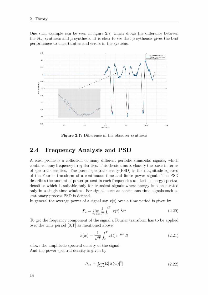
One such example can be seen in figure 2.7, which shows the difference betweenthe H∞ synthesis and µ synthesis. It is clear to see that µ sythensis gives the bestperformance to uncertainties and errors in the systems.

Figure 2.7: Difference in the observer synthesis

2.4 Frequency Analysis and PSDA road profile is a collection of many different periodic sinusoidal signals, whichcontains many frequency irregularities. This thesis aims to classify the roads in termsof spectral densities. The power spectral density(PSD) is the magnitude squaredof the Fourier transform of a continuous time and finite power signal. The PSDdescribes the amount of power present in each frequencies unlike the energy spectraldensities which is suitable only for transient signals where energy is concentratedonly in a single time window. For signals such as continuous time signals such asstationary process PSD is defined.In general the average power of a signal say x(t) over a time period is given by

Px = limT 7→∞

1T

∫ T

0|x(t)|2dt (2.20)

To get the frequency component of the signal a Fourier transform has to be appliedover the time period [0,T] as mentioned above.

x(w) = 1√T

∫ T

0x(t)e−jwtdt (2.21)

shows the amplitude spectral density of the signal.And the power spectral density is given by

Sxx = limT 7→∞

E[|x(w)|2] (2.22)

14

2. Theory

where, E is the expected value given by the Fourier transform

E[|x(w)|2] = 1T

∫ T

0

∫ T

0E[x∗(t)x(t′)]e−jw(t−t′)dtdt′ (2.23)

Eqn 2.23 represents the auto-correlation function of the signal x(t)

Rxx(τ) = (X(t)∗X(t+ τ)) (2.24)

PSD is defined by the auto-correlation function by

Sxx =∫ T

0Rxx(τ)e−jwτdτ = Rxx(w) (2.25)

provided Rxx(τ) is integrable.

15

2. Theory

16

3Methodology

3.1 Model Based Estimation AlgorithmThe design methodology implemented in this thesis is shown in figure 3.1.

Verticaldynamics

Road profileestimation

Transformationto space domain

Power spectraldensity

Classifier

Descisionlevel

Averagingwith moremeasurements

RoadClass

Profile Estimation

Frequency Analysis

ISO 8608Classfication

Cloud storage

Figure 3.1: Methodolgy

As seen from the figure above the process involves estimation of the road profile andclassification obtained from the sensor data of a vehicle with semi-active suspensionsystem

• Profile Estimation : To estimate the suspension parameters usingH∞observeras discussed in section 2 and thereafter estimate the road profile based on thestatic equation of the unsprung mass accelerations (2.8).

• Frequency analysis : By using the profile estimate in the time domain,Frequency components of the road signals is determined and the correspondingpower acquired in each frequency is determined.

• ISO 8608 Classification : Classification standard of the type of roads basedon power spectral densities. Given an idea about the road surface irregularity.

17

3. Methodology

The quarter car model represented as state space representation is used for theestimation of road profile. The best way to understand the performance of a modelfor respective inputs is through the singular value of frequency response of thesystem. The linear plant model dynamics with road and damper force as inputs canbe can be seen in figure 3.2.

10-1

100

101

102

103

-100

-50

0

50

100

150

200

250

semi-active suspesion

passive suspension

Singular Values

Frequency (Hz)

Sin

gula

r V

alu

es (

dB

)

Figure 3.2: System dynamic of semi active suspension with passive suspensionsystem

Figure 3.2 also shows the difference between the semi-active suspension and thepassive suspension system. Since the damper force is considered as a continuouslychanging input to the model and not included in the state space dynamic modelwe can observe the invariant peaks at two frequencies. The figure shows two plotsobtained from the two inputs. The plot with higher singular values is due to theroad input on body displacement and the other is due to the damper force input onthe body displacement. The transfer function between damper force input to thebody displacement and velocity has imaginary zeros with resonance at 73.84rad/s(12Hz), this frequency is called the wheel hop frequency. And the transfer functionbetween the suspension deflection and damper force produces imaginary zero withresonance at 20.82rad/s(3Hz) is called the rattle space frequency.

Hence in a semi-active suspension system it is assumed to have an actuator con-nected between unsprung and sprung mass to control the suspension over completebandwidth of the two frequencies, to provide a better ride performance. In case ofthe passive suspension system, since there is no assumption of controlled damperforce between the two masses, the peaks at the two frequencies are highly damped.

The overall estimation model of a closed loop structure with an observer as a feed-back and control inputs are estimated states as outputs is then built.

18

3. Methodology

Wzr

WFd

Wei

Wd

LTI plant model (G)

H∞observer(K)

zr

Fd

ze = x− x

nx

y

Systeminterconnection

Figure 3.3: H∞ Estimation method

Optimized observer is synthesized in order to make the H∞norm as low as possi-ble. To obtain this condition three weighting functions are added to the plant forloop shaping as shown in figure 3.3. A loop-shaping technique to design perfor-mance filters in the optimization setting is used for the observer design. This thesisdoes not deal with robustness issues with a controller design and focuses more onH∞optimization to the frequency dependant loop-shaping state observers. The op-timized state observer estimates the suspension parameters as control inputs fedback to the plant model which in turn minimizes the error dynamics and reducingthe effect of the measurement noise.

The filter specifications used in the design of H∞observer is explained below. Find-ing an appropriate weighting function is a crucial step in the robust control designwhich requires few trials.

From fig 3.3 the weighting matrix denoted by Wzr is the loop shaping transfer func-tion responsible to shape the irregularities of the road in the frequency band ofinterest. This is shown in 3.4. The road variability consists of slow changing profilesand high frequency irregularities, a relevant part of the road spectrum is a suitablechoice to affect the dynamics of the vehicle. The slow variability in the road profileless than 0.01 cycles/m (0.3Hz) or wavelength above 100 m and similarly the highfrequency irregularities greater that 5 cycles/m (30Hz) or wavelength below 0.5mare filtered out since it is difficult to measure high frequencies with the sensors usedand very low frequencies do not affect the vehicle dynamics, hence they are notincluded in the spectrum. The region covered with boundary in the red color showsthe region of interest.

19

3. Methodology

10-4

10-3

10-2

10-1

100

101

102

103

4

5

6

7

8

9

10

11

12

13

Road shaping filter

Wzr

Frequency (Hz)

Sin

gula

r V

alu

es (

dB

)

Region of interest

Figure 3.4: Road shaping filter

The actuator CCD model is an approximation of the behaviour the physical sys-tem which accounts for varying displacements and modelling errors. There existsa nominal behaviour with frequency dependant amount of uncertainty. At lowerfrequency around 0.1Hz a 40% uncertainty of the nominal model is applied and atfrequency greater than 3Hz the uncertainty is greater than 100% of the nominalvalue. An input multiplicative uncertainty model is developed as a weighting to theactuator which can be seen in figure 3.5. The nominal model is represented withblack color in the right half of the figure. The uncertainties shown are respectiveto that nominal model. These input uncertainties are included in the filter designsince factors such as change in current reading due to external parameters such astemperatures or small displacement errors in the deflection velocity brings changesin the damper force. Therefore to account for this changes an input multiplicativeuncertainty is considered for the actuator model.

10-2

10-1

100

101

102

103

104

105

-120

-100

-80

-60

-40

-20

0

20

nominal filter

unceratinty

Singular Values

Frequency (Hz)

Sin

gula

r V

alu

es (

dB

)

Figure 3.5: Actuator uncertainty model

Another weighting from the figure 3.3 represents the performance weightings. Itis used in the minimization of the estimation error in the frequency region of the

20

3. Methodology

suspension operation. To achieve a desired performance of noise reduction it isnecessary to satisfy the inequality condition ||Wei(I +GK)−1||∞ < 1. The singularvalues of the sensitivity function (I + GK)−1 must lie below the inverse of theweighting function ( 1

Wei) for all frequencies as shown in figure 3.6. Hence a precisely

tuned performance weighting has to be chosen

10-4

10-2

100

102

104

106

-60

-40

-20

0

20

40

60

80

100

120

Inverse performance

sensitivity

Singular Values

Frequency (Hz)

Sin

gula

r V

alu

es (

dB

)

Figure 3.6: Choice of performance weightings against the sensitivity

In general case, the measurement noise is a complementary sensitivity function froma classical closed loop transfer equation 3.1 which describes that less weightage isgiven to the noise signals which are generally present in the higher frequencies ofthe sensor signals.

y = (I +GK)−1GK︸ ︷︷ ︸T

r + (I +GK)−1︸ ︷︷ ︸S

Gdd− (I +GK)−1GK︸ ︷︷ ︸T

n (3.1)

100

102

104

-80

-70

-60

-50

-40

-30

-20

-10

Wn1

Frequency (Hz)

Sin

gula

r V

alu

es (

dB

)

100

102

104

-80

-70

-60

-50

-40

-30

-20

-10

Wn2

Frequency (Hz)

Sin

gula

r V

alu

es (

dB

)

100

102

104

-70

-60

-50

-40

-30

-20

-10

0

Wn3

Frequency (Hz)

Sin

gula

r V

alu

es (

dB

)

Figure 3.7: Weighted noise measurements

All these filters are used in support of loop shaping techniques to operate the systemin the frequency region of interest. Whereas, for lower frequencies which includes

21

3. Methodology

slower dynamics of the road it might account to small drift from an accelerometersensor. The structure of the open loop system is then interconnected with all theweightings. By taking into account the the performance outputs and weights given

[zy

]= P

d1d2u

(3.2)

Here d1 is an input to the weighting matrices Win = diag(WFd,Wzr), d2 is thedisturbance input to Wd and u = x the control input.By using the equations for inputs and outputs i.e the performance output and themeasurement output

z = WeiGWind1 −Weiu

y = GWind1 +Wdd2(3.3)

the interconnected block P will take the form[zy

]=[WeiGWin 0 −Wei

GWin Wd 0

] d1d2u

(3.4)

where,

P =[WeiGWin 0 −Wei

GWin Wd 0

](3.5)

The system interconnected block P is then used in the H∞ synthesis with measure-ments as inputs and estimated states as the number of outputs System interconnec-tion can also be done by using sysic command from the MATLAB.

3.2 Power Spectral DensityRoad profile data zr(t) is converted to frequency domain by using Fourier trans-formation to determine the frequency components of the signal. By knowing thevehicle velocity equivalent road profile zr(x) is determined in spatial domain andspatial angular frequency domain can also be determined, since space domain is thebest way to classify the roads according to ISO 8608 classification.

By using a Matlab function "pwelch" it is possible to determine the power spectraldensity of the spatial domain signal directly. This uses a similar method as explainedin section 2.4 The pwelch() method uses a moving window technique where FFT iscomputed and then PSD is computed as average of FFT’s over all windows. Thismethod is dependant on three parameters.

• Window length (N) : The convention of choosing the window size N is set tothe power of 2 greater than the length of the signal. But this procedure wouldmake it less efficient and faster implementation of the FFT. If N is less than

22

3. Methodology

the length of the signal then FFT will utilize only N samples to estimate thePSD. An effective utilization of the window size is to be chosen such that thenumber of windows used over the data is effective. This will help in obtaininga smooth PSD. Frequency resolution (distance between two frequency points)is another factor that should be taken care of such that important frequencycomponents are not lost.A suitable window size is chosen in this thesis considering 2000 samples persecond of signals of varying length. By using a window function such as Ham-ming window it is possible to have very less side-lobes and makes it betteroption for frequency selective analysis.

• Overlap percentage : The change in the overlap percentage varies the effectsof noise in the signal. Lower overlap percentage with 0% increases the overallnoise in the PSD, and with increase in the overlap percentage to 50% increasesthe number of windows and helps in the averaging of the effects of noise.Increasing it further to 100%, the correlation between the windows samplesincreases, thus averaging brings no effect on the noise.Therefore 50% noise is taken into consideration

• Number of FFT points : The number of FFT points chosen is equal to thelength of the window

3.2.1 ISO 8608 Classification

ISO is a worldwide federation of national standards designated to form standards ofrules for the specified work. The committee responsible for the document related toroad classification is "Mechanical vibration, shock and condition monitoring". Theroad profile classification is done by standards mentioned in the ISO 8608 [25]. Thepower spectral density of a road profile is defined by

Gq(n) = Gq(n0)(n

n0

)−w(3.6)

n is the spatial frequency and n0 is the reference spatial frequency of 0.1m−1 andGq(n) is the power spectral density at spatial frequency n. The reference PSDGq(n0) determines the differences in the road classes, where smallest value showsbetter roads and greater values the bad roads. w represents the waviness of theroad with greater values of w representing higher amplitudes and lower frequencyand smaller values of w representing higher frequency and lower amplitudes. ButISO 8608 uses w=2 as the waviness.The ISO road level definition is given by

23

3. Methodology

Road Class Gq(n0)10−6m3

A 16B 64C 256D 1024E 4096F 16,384

Table 3.1: Road level definition by ISO

The representation of all the classes from A to F with values given in table 3.1 canbe seen in the figure 3.8. The road profile estimates will be described by the PSDof its vertical displacement. As seen in the figure 3.8 the PSD is in m3 versus thespatial frequency in cycles/m are on the logarithmic scale. The below figure alsorepresents the fitted PSD which describes the region around the type of road.

Since the spatial frequency range is important for vehicle dynamics analysis, therange for which is chosen between nε[0.01 4]cycles/m.

Figure 3.8: Classification of roads from A to F

For the vehicle driven at a velocity of V ms−1 the spatial PSD can be transformedinto time domain PSD as in equation 3.7

Gq(f) = 1vGq(n) = Gq(n0)n2

0Vf 2 (3.7)

where f is the frequency in Hz. The relation between the excitation energy of thePSD coefficient Gq(n0)n2

0 and the vehicle velocity can be seen in 3.9. The figureshows that the increase in vehicle velocity increases the the roughness coefficient.Therefore, the vehicle velocity is directly proportional to the roughness coefficient.

24

3. Methodology

Figure 3.9: Roughness coefficient vs velocity

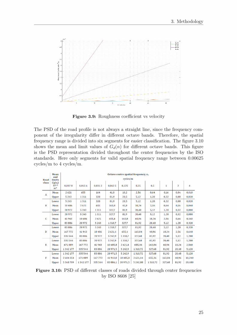
The PSD of the road profile is not always a straight line, since the frequency com-ponent of the irregularity differ in different octave bands. Therefore, the spatialfrequency range is divided into six segments for easier classification. The figure 3.10shows the mean and limit values of Gd(n) for different octave bands. This figureis the PSD representation divided throughout the center frequencies by the ISOstandards. Here only segments for valid spatial frequency range between 0.00625cycles/m to 4 cycles/m.

Figure 3.10: PSD of different classes of roads divided through center frequenciesby ISO 8608 [25]

25

3. Methodology

26

4Results

The results of the estimation and the classification for the roads are presented inthis section. Results are divided into simulation results i.e testing it on the Car-Maker and experimental results (sensor data collected by driving the vehicle on testtracks). High frequency roads and low frequency roads are both part of the experi-mental result structure. In the experimental data, the speed of the vehicle is almostmaintained as a constant. Later a classification study is done comparing the roadswith the ISO standard roads. The effect of these on the primary ride and secondaryride is also studied and definition of how it helps in the damping control is alsoanalyzed.The available tools and sensors used during this thesis are limited to existing vehiclesensors. The effect of this limitation is studied and the results are discussed.

4.1 Estimation Results

4.1.1 CarMakerCarMaker is a software tool which consists of entire vehicle dynamics comprisingof suspension, vertical, lateral, longitudinal and tire dynamics. Hence the obtainedresults will be considered to be behaving very close to the CarMaker data. Therefore,the roads are considered from this software for testing.The road models from CarMaker is used in order to test the estimation results.Several road conditions are included in order to determine the classification on thetype of the road to be determined. High frequency disturbance roads and roadshaving very slow change in the topography i.e low frequency disturbance are someof the roads used for the classification.Whilst having the road model built, there are certain parameters needed to be setin the CarMaker.

• Maneuvering : The speed at which the vehicle moves on the road profile is sethere. To account offset of the vehicle position is also set here.

• Road bumps : The road bumps are set in the parameters section. Beams orwaves is chosen to test in order to have single or multiple bumps. Anotheroption used is a CRG file i,e a built in model of certain roads which replicatethe real road scenario is also chosen.

• Vehicle Parameters : Mass of the vehicle, suspension parameters are neededto be set.

• Sensors : For obtaining the measurements from the maneuver of the vehicle,

27

4. Results

respective sensors such as body accelerometers and position sensors placed inthe vehicle are used.

4.1.2 Estimation of suspension parametersThe suspension parameters comprising of the states used to determine the road pro-file is estimated here. CarMaker software tool as explained above is used to verifyand analyze the estimated parameters of the suspension from the observations. Theobserver is built by considering measurements used from the vehicle sensor data.The mounted senors provide information about the suspension behaviour in realtime which is useful in validation and verification of the estimates. In order to firstvalidate the observer, measurements are chosen from the linear model and tested, theresults for which can be seen in figure 4.1. Different bumps and symmetrical/unsym-metrical roads are part of the result. The car in the simulation is run at a differentspeeds, On the wavy road (a) the vehicle speed is 50kmph, Unsymmetrical waves(b)at 35kmph, Road roughness(c) at 30kmph and on Belgian road(d) at 70kmph. Themeasurements sprung deflection and velocity and the sprung mass accelerations arechosen from the linear model and given as an input to the observer. The outputs arethe state estimates sprung mass displacements zs, sprung mass velocity ˆzs, unsprungmass displacement zus, and unsprung mass velocity ˆzus. The linear model outputsare shown in blue and the estimates are in red.

(a) Waves (b) Unsymmetrical Waves

(c) Road Roughness (d) Belgian Road

Figure 4.1: Estimates for CarMaker demo road surfaces with linear model

The same observer is tested with the non-linear model from the CarMaker, theresults for which can be seen below. The results show the states matches preciselywith that of the CarMaker sensor data. These are further used in estimation of theroad profile. Figure 4.2 shows the similar roads tested with the linear model. Thevehicle speed is the same as used for verification with the linear model.

28

4. Results

(a) Waves (b) Unsymmetrical Waves

(c) Road Roughness (d) Belgian Road

Figure 4.2: Estimates for CarMaker demo road surfaces with nonlinear model

Two roads are further chosen to compare and analyze the road estimate and thefrequency components of the profile. The roads chosen are the best example tostudy the effects of the road irregularities affecting the control of the damper as aresult of the ride quality. The two roads are given the names Road A and roadB. They have symmetrical and unsymmetrical wavelengths of profile irregularitieswhich could be distinguished by the frequency components.Road A has track width of 3m and driven on the center lane with no offset. Thelength of entire road is around 550m and the vehicle is driven at a speed of 65 kmph.Road B has a track width of 3m and driven on center lane without any offset. Thelength of the road is around 300m and speed of the vehicle is 70 kmph. Figures 4.3and 4.4 shows the state estimates of Road A and Road B in comparison with actualstate values from the CarMaker.

Figure 4.3: Suspension parameters estimate for road A

29

4. Results

Figure 4.4: Suspension parameters estimate for road B

Further these estimates are used to construct the road profile, which is presented inthe next section.

30

4. Results

4.1.3 Road Estimation ModelThe road estimation is done based on the estimations obtained from the observer.The profile estimate obtained is a proximity of the real road profile. Since theunsprung mass accelerometer is not a part of the observed vehicle measurement, Itis determined from the estimated states by taking the derivative of the unsprungvelocity and then filtered to obtain the data only from the range of interest.Equation 2.8 is used to estimate the road profile. The estimated unsprung massaccelerations ˆzus for the two roads A and B is shown in figure 4.5 and 4.6.

15 20 25 30 35 40 45 50 55

time(s)

-15

-10

-5

0

5

10

15

Unspru

ng m

ass a

ccele

rations (

m/s

^2)

Time Series Plot:

CarMaker unsprung acceleration

Estimated unsprung acceleration

37 38 39 40 41-6

-4

-2

0

2

4

Figure 4.5: Unsprung mass acceleration for road A

5 10 15 20 25 30 35 40 45 50 55 60

time(s)

-60

-50

-40

-30

-20

-10

0

10

20

Unspru

ng m

ass a

ccele

rations (

m/s

^2)

Time Series Plot:

CarMaker unsprung acceleration

Estimated unsprung acceleration

37 38 39 40 41-10

-5

0

5

10

15

Figure 4.6: Unsprung mass acceleration for road B

The road profile zr(t) shown is in the time domain, therefore, with the speed ofthe vehicle it is possible to determine an equivalent road profile zr(x) as a functionof the road length x. The estimate is then passed through a moving average filterwhich acts as a simple low pass(FIR) filter. A suitable filter length is chosen suchthat any important modulations in the profile data is not affected. Road estimatefor road A is shown in 4.7 and road B is shown in 4.8

31

4. Results

0 10 20 30 40 50 60

time (s)

-0.3

-0.25

-0.2

-0.15

-0.1

-0.05

0

0.05

0.1

Pro

file

Heig

ht (m

)

Estimated

road

Figure 4.7: Road profile estimate for road A

10 15 20 25 30 35 40 45 50 55

time (s)

-0.2

-0.15

-0.1

-0.05

0

0.05

0.1

0.15

0.2

0.25

Pro

file

Heig

ht (m

)

Estimated

road

Figure 4.8: Road profile estimate for road B

32

4. Results

4.2 Frequency Analysis and Power spectrum den-sity

Frequency analysis is carried out for the road estimates in the previous subsection4.1. It is necessary to study the frequency components of these roads as they buildthe notion of any prolonged disturbances from the road, which could be plausibleharm to the vehicle or human body. They even provide information for the controlof the vehicle suspension on a specific length of the road, helping in improving theride quality and the handling of the car. Human body is another such complexstructure with different organs resonating at different frequencies. Hence knowingthe frequency components of the road is vital aspect of vehicle dynamics.

10-1

100

cycles/m

10-9

10-8

10-7

10-6

10-5

10-4

10-3

10-2

10-1

100

PS

D(m

3)

CarMaker road profile PSD

Estimated road profile PSD

X: 0.05307

Y: 0.003141

Figure 4.9: PSD comparison for Road A

10-1

100

cycles/m

10-9

10-8

10-7

10-6

10-5

10-4

10-3

10-2

PS

D(m

3)

CarMaker road profile PSD

Estimated road profile PSDX: 0.03708

Y: 0.006862X: 0.06181

Y: 0.001513

Figure 4.10: PSD comparison for Road B

Since the scope of the thesis remains to classify these roads based on its condition,

33

4. Results

power spectral density is the best way to define the road’s spatial frequency compo-nent because it is independent of the velocity of the vehicle. The PSD for Road Ashown in figure 4.9 clearly represents a low frequency disturbance in the road with apeak around 0.053 cycles/m, with the vehicle moving at a velocity of 75 kmph andthe PSD for road B is shown in 4.10 with multiple frequency disturbances with peaksat 0.03 cycles/m and 0.06 cycles/m. The figures also show the comparison betweenthe real road profile from the CarMaker road sensor data and the estimated roadprofile. It is clear to see the similarities between the estimated spectral densities.

The vehicles travelling on a single lane won’t always be travelling in the same widthof the track. For example if a lane has a width of 3m, the vehicle might travel withsome offset of 0.5m, 1m or greater. A test is done to check the similar circumstance.Road A is considered for this. Figure 4.11 shows the vehicle travelled on the sametrack but having some offsets in the track position. The offset of 1m is set for thecar position. Although the PSD of the shown road profile almost remains the same.The power spectral density of road with an offset shown is for the left wheel, similarexperiment is carried out with an observer at the right wheel.

10-1

100

cycles/m

10-9

10-8

10-7

10-6

10-5

10-4

10-3

10-2

10-1

100

PS

D(m

3)

No track offset

1m track offset

Figure 4.11: PSD comparison for offsets

The spatial frequency is used in the ISO standard classification of the roads and theimportance of representing the spectral density in spatial frequency can be seen fromfigure 4.12. Road A is considered in this case as well. The vehicle is driven on thesame track at different speeds i.e 48kmph, 75kmph, 90kmph, 120kmph and 150kmph.Since moving at different speeds on the same road profiles would have different timedomain frequency disturbance, whereas the spatial frequency would show the samepeak for all varying velocities which is easy to understand and represent. Althoughthere arises few differences when vehicle is moving at higher speeds which is due tothe suspension settings on the vehicle. Comparison with the ISO standards is shownin the appendix.

34

4. Results

10-1

100

cycles/m

10-9

10-8

10-7

10-6

10-5

10-4

10-3

10-2

10-1

100

PS

D(m

3)

48kmph

75kmph

90kmph

120kmph

150kmph

Figure 4.12: PSD comparison at varying speeds

4.3 Experimental resultsSection 4.2 explains about the examples considering the measurements form the Car-Maker sensor data. This would still consider an ideal case in real world with veryless uncertainties and disturbances. Therefore, real world measurements are col-lected from the sensors placed on vehicle and driven on test tracks. Similar observermodel is used for estimation of the states using these sensor measurements withmore uncertainties and disturbances present in them. The measurements sprungmass accelerations zs and suspension deflection zdef from the sensors are sampled at2000Hz and an offline estimation is done in Simulink. These measurements sprungmass acceleration is low pass filtered at 30Hz to include the region of interest forthe dynamics. This filtered data in turn removes additional noise affecting the esti-mation. In turn the deflecting velocity of the suspension which is differentiated andfiltered from the suspension deflection data is another measurement passed as aninput to the observer.

Different examples of various roads are provided below. These are the roads from theexperimental test tracks. The suspension estimates and the respective road profilesare shown. The unsprung mass acceleration used in determining the road estimatesare obtained from the suspension estimates.

35

4. Results

Figure 4.13 and 4.14 represents the state and road estimates respectively for roadwith manholes on the left side of the track present at a distance of 40m approxi-mately. It shows that the amplitude is quite small which makes the sprung massmovement very negligible compared to the unsprung mass movement.

Figure 4.13: Suspension parameter estimate for manhole road

The road estimates shows very such small dips representing profile irregularity.

2 4 6 8 10 12

time(s)

-0.1

0

0.1

0.2

0.3

0.4

0.5

0.6

0.7

Pro

file

he

igh

t(m

)

Figure 4.14: Road estimate for manhole road

36

4. Results

Figure 4.15 and 4.16 represents the state and road estimates respectively for roadwith roll excitation on left side of the track. It shows a constant dip at an equidistantdistance. These roads create discomfort when the vehicle body rolls to the left. Sincethe measurements used are limited and the vehicle roll is not plotted here.

Figure 4.15: Suspension parameter estimate for roll excitation on Front left wheel

The road estimates shows the dips from the left wheel representing profile irregu-larity.

5 10 15 20 25 30 35

time(s)

-0.2

-0.15

-0.1

-0.05

0

0.05

0.1

0.15

0.2

Pro

file

he

igh

t(m

)

Figure 4.16: Road estimate for roll excitation on front left wheel

37

4. Results

Figure 4.17 and 4.18 represents the state and road estimates respectively for roadwith low dips at equidistant distance. These are the low frequency disturbancesaffecting the primary rides in vehicle dynamics. These roads are similar to road Aof the section 4.2.

Figure 4.17: Suspension parameter estimate for low frequency road

The road estimates shows the low frequency long dips representing profile irregular-ity.

5 10 15 20 25 30 35 40 45 50 55 60

time(s)

-1

-0.5

0

0.5

1

Pro

file

he

igh

t(m

)

Figure 4.18: Road estimate for low frequency road

38

4. Results

Figure 4.19 and 4.20 represents the state and road estimates respectively for roadwith high frequency disturbances which affects the secondary ride in vehicle dynam-ics. These roads have unsymmetric wavelengths of road profiles.

Figure 4.19: Suspension parameter estimate for high frequency road

The road estimates shows high frequency profile irregularity.

0 5 10 15 20 25 30 35 40 45 50

time(s)

-0.5

-0.4

-0.3

-0.2

-0.1

0

0.1

0.2

0.3

Pro

file

he

igh

t(m

)

Figure 4.20: Road estimate for high frequency road

39

4. Results

4.3.1 Frequency analysis and PSD for Experimental dataTwo roads representing low frequency and high frequency disturbance i.e road es-timates from figures 4.18 and 4.20 are considered. Frequency components of thesetwo roads can be seen below.

0 5 10 15 20 25 30

Frequency (Hz)

-20

-10

0

10

20

30

40

50

60

70

80

Magnitude (

dB

)

Magnitude Response (dB)

Frequency: 0.7324219

Magnitude: 51.07753

(a) Symmetric Wavelength

0 5 10 15 20 25 30 35 40 45

Frequency (Hz)

-30

-20

-10

0

10

20

30

40

50

60

Magnitude (

dB

)

Magnitude Response (dB)

Frequency: 14.03809

Magnitude: 36.62762

(b) Random wavelength

Figure 4.21: Primary and secondary ride roads

As already discussed the power spectral density in spatial domain is the region ofinterest, further results will feature comparison of the spectral density in units ofwavenumber. One road to easily compare the data from CarMaker and experimentaldata is the low frequency road. Figure 4.22 show the PSD of the roads, althoughat higher frequencies few uncertainties and different damping controls might be fewreasons of small differences. The peak obtained from CarMaker is at 0.058 cycles/mand the peak obtained from the experimental data is at 0.06 cycles/m which showsnot much difference between them. This would be an ideal case for the classificationof road.

Figure 4.22: Comparison between CarMaker PSD estimate and experimental PSDestimate

In order to verify power spectral density of the experimental data for high frequencyroad, the car is driven on the same track twice first at 60kmph and then 70kmph, theresult of which can be seen in the 4.23. The figure shows the PSD for the same roadwidth for left and right wheel. The result shows that the power spectral densities of

40

4. Results

the same road matches hence it could be useful for classification of the type of theroad.

10-1

100

cycles/m

10-10

10-9

10-8

10-7

10-6

10-5

10-4

10-3

10-2

10-1

PS

D(m

3)

PSD for left wheel

PSD for right wheel

Figure 4.23: PSD comparison when driven on same road back and forth

4.3.2 ISO ClassificationThe power spectral densities of the road estimates is compared to ISO standardsas explained in the section 3.2.1. This makes it easier to classify the roads atdifferent spatial frequency and provide an idea for the control of the dampers. Figure4.24 shows the PSD for low frequency roads on the fitted PSD classes of the ISOstandards. The low frequency road is the experimental road estimate representedin figure 4.18. The peak frequency in spatial domain is around 0.06 cycles/m or0.74Hz with the vehicle travelling at 15.5 m/s.

Figure 4.24: Displacement PSD of low frequency road

In figure 4.25(a) shows type of classes for all points of spectral density in spatial fre-quency range and 4.25(b) shows the peak frequency at a particular central frequency

41

4. Results

of in the spatial frequency octave bands. The central frequencies for division intofrequency segments is given in figure 3.10. The classification based on the centralfrequency will provide clear information for setting the damper control for primaryand the secondary ride. As it can be seen the the central frequency 0.06 cycles/mshows the peak for the low frequency disturbance.

0 0.5 1 1.5 2 2.5 3

cycles/m

ISO-A

ISO-B

ISO-C

ISO-D

ISO-E

ISO-F

ISO

road c

lasses

(a) PSD for specified frequencies

0 0.5 1 1.5 2 2.5 3 3.5 4 4.5

cycles/m

ISO-A

ISO-B

ISO-C

ISO-D

ISO-E

ISO-F

ISO

road c

lasses

(b) PSD only for central frequencies

Figure 4.25: Primary and secondary ride roads

The parameters for such classification can be seen in table 4.1. The standard of theroad is said to be ISO-C class at lower frequencies.

RMS speed 15.5 m/sPeak Frequency 0.74 HzSpatial frequency 0.06 cycles/m

Road Class ISO-C

Table 4.1: Parameters of low frequency road classification

Similarly, figure A.1 shows the PSD of high frequency road on the fitted ISO stan-dards, The high frequency road is the experimental road one shown in figure A.1.The peak frequency is at 1.075 cycles/m or 14.03 Hz. The velocity of the vehiclemoving is at 14 m/s.

42

4. Results

Figure 4.26: Displacement PSD of high frequency road

In figure 4.27(a) shows type of classes for all points of spectral density and 4.27(b)shows the peak frequency at a particular central frequency of in the spatial frequencyoctave bands. The parameters of such classification can be seen in table 4.2. It canbe seen that the peak can be seen for a central frequency of around 1 cycle/m.

0 0.5 1 1.5 2 2.5 3

cycles/m

ISO-A

ISO-B

ISO-C

ISO-D

ISO-E

ISO-F

ISO

road c

lasses

(a) Symmetric Wavelength

0 0.5 1 1.5 2 2.5 3 3.5 4 4.5

cycles/m

ISO-A

ISO-B

ISO-C

ISO-D

ISO-E

ISO-F

ISO

road c

lasses

(b) Random wavelength

Figure 4.27: Primary and secondary ride roads

The parameters for this classification can be seen in table 4.2. The standard of theroad is said to be ISO-F class at higher frequencies.

RMS speed 14 m/sPeak Frequency 14.03 HzSpatial frequency 1.075 cycles/m

Road Class ISO-F

Table 4.2: Parameters of high frequency road classification

Similarly, classification could be done for all the estimated road profile based on thePSD as given by the ISO standardization. Meanwhile the ISO standardized classi-fication considers the waviness of any type of road to be fixed at 2. A classification

43

4. Results

algorithm to include different waviness for different roads is included in the futurescope.

44

4. Results

4.3.3 Decision for Damper tuning for Primary and Secondaryride

The operation condition of a vehicle is subjected to many vibrations in the vehiclebody caused by many things at different frequencies. The vibration that createsdiscomfort to passengers can be distinguished by different ways as seen in figure4.28

Figure 4.28: Maneuvering frequency ranges

In automotive industry the ride behaviour is described by primary and secondaryride. The primary ride would describe the road with bumps having higher ampli-tudes and lower frequencies. Such topographic variation would be visible to thenaked eye whilst driving. Such riding conditions of the road is termed as the pri-mary ride. Which includes suspension movement over undulations related to thebound and rebound of the dampers.

Secondary ride is small irregularities with low amplitudes but higher frequenciesWhich is slightly difficult to be seen from the moving vehicle. Such irregularities aremainly due to combination of damper and bushing control. The tuning in secondaryride involves the dampers and bushings to work well.

The frequency content of the primary ride is less than 6Hz, with the wavelengthgreater than the wheel base of the vehicle. These roads mostly have symmetricprofile. An example of such road profile can be seen in figure 4.29(a) The fre-quency component of the secondary ride has medium frequency range around 8Hzand greater. The irregularities in the road profile is continuously varying in largespectrum of wavelengths. This can be seen in figure 4.29(b)

45

4. Results

(a) Symmetric Wavelength (b) Random wavelength

Figure 4.29: Primary and secondary ride roads

Influence of the low frequency and high frequency roads from the results on primaryand secondary ride can be

• Low frequency roads in the primary ride must have a suspension dampingincreased to get better damping at frequencies below 6Hz which eliminatesthe peak frequencies in that region and improves the ride quality. But withsame settings if the vehicle is driven on the high frequency roads then the ridequality is deteriorated causing a slower roll-off and harshness.

• High frequency roads in the secondary ride must have a suspension dampingdecreased to get better damping at higher frequencies from 8Hz to above elim-inating the peak frequencies improve the ride quality. If with same setting thevehicle is driven on low frequencies then it will have a large impact on thepassenger.

46

4. Results

4.4 Future Scope• The suspension parameter estimation uses a quarter car model which operates

in a lower frequency region where the accelerometer data tends to drift with avery slow varying slope, hence a full car model can be used to build an observerto handle the case of slow varying topographies.

• The estimated states can also be used to the control the damper force.• Here a classification is done using a continuous time observer model. An online

estimation can be done by discretising the model and the observer at a specificsampling rate.

• The ISO classification uses the waviness of the road to be 2 for all sets ofroad. A different classification standards could be considered for varying setsof waviness of the roads depending on the reference classes of the road.

47

4. Results

48

5Conclusion

The main objective of this thesis was to to estimate the road profile and classifythe road based on the roughness of the road. The first chapter introduced manytechniques used in the current market for estimation of the classes of the road androad profile. Response based road profile estimation was the one considered. Thesecond chapter gives insight into the vehicle modeling. The continuous damper inthe semi-active suspension model is explained along with a quarter car model ofthe left wheel suspension model. Road profile estimation model is also defined. Therobust observer H∞model is derived for the estimation of the suspension parameterslater used to estimate the road profile. The third chapter explains about the methodin which the estimation and classification is done. The choice of filter specificationsand loop shaping for the robust observer is explained. The ISO standards for classi-fication of the road profile based on power spectral density in the spatial frequencydomain is introduced. The last chapter is used to explain the results obtained fromthe simulations from Carmaker data and the experimental results from the sensordata collected from the measurements run on the test tracks.

49

5. Conclusion

50

Bibliography

[1] DGIP. EU road surfaces: Economic and safety impact of the lack of regularroad maintenance, study. Policy Department Structural and Cohesion Policies,European Parliament,2014.

[2] S. Gerwens. European Manifesto: Need for road maintenance. Pavement Preser-vation and Recycling, Summit, 2015.

[3] US department of transportation. Long-term pavement performance program[4] Z. Zhang, C. Sun, R. Bridgelall, et al. Application of a machine learn-

ing method to evaluate road roughness from connected vehicles. Journal ofTransportation Engineering, Part B: Pavements, 144(4):04018043, 2018. DOI:10.1061/jpeodx.0000074.

[5] R. Bridgelall, Y. Huang, Z. Zhang, et al. Precision enhancement of pavementroughness localization with connected vehicles. Measurement Science and Tech-nology, 27(2):025012, 2016. DOI: 10.1088/0957-0233/27/2/025012

[6] Y. Qin, M. Dong, F. Zhao, et al. Comprehensive analysis for influence of control-lable damper time delay on semi-active suspension control strategies. Journalof Vibration and Acoustics Transactions of ASME, 139(6):031006, 2017. DOI:10.1115/1.4035700.

[7] K. Mcghee. Automated pavement distress collection techniques. TransportationResearch Board, 2004.

[8] H. Imine, Y. Delanne, and N. K. M’sirdi. Road profile input estimation invehicle dynamics simulation. Vehicle System Dynamics, 44(4):285–303, 2006.DOI:10.1080/00423110500333840.

[9] Acuity AR600/RP: Laser displacement sensor for road profilometry.https://www.Acuitylaser.Com/Docs/Ar600-Road-Profiling.Pdf

[10] M. Ahmed and F. Svaricek. Preview optimal control of vehicle semi-active sus-pension based on partitioning of chassis acceleration and tire load spectra. Proc.of the Control Conference (ECC), 2014. DOI: 10.1109/ecc.2014.6862615.

[11] Z. Yuan, X. Zhang, S. Liu, et al. Laser line recognition for autonomous roadroughness measurement. Proc. of the Cyber Technology in Automation, Con-trol, and Intelligent Systems (Cyber), 2015. DOI: 10.1109/cyber.2015.7287977.

[12] M. Aki, T. Rojanaarpa, K. Nakano, et al. Road surface recognition using laserradar for automatic platooning. IEEE Transactions on Intelligent Transporta-tion Systems, 17(10):2800–2810, 2016. DOI: 10.1109/tits.2016.2528892.

[13] D. Hrovat and W. Tseng. Adaptive active vehicle suspension system. USPatents. 1995.

[14] K. Yi and B. Song. A new adaptive sky-hook control of vehiclesemi-active suspensions.Proc. of the Institution of Mechanical Engineers,

51

Bibliography

Part D: Journal of Automobile Engineering, 213(3):293–303, 1999. DOI:10.1243/0954407991526874.

[15] H. Imine, Y. Delanne, and N. K. M’sirdi. Road profile input estimation invehicle dynamics simulation. Vehicle System Dynamics, 44(4):285–303, 2006.DOI: 10.1080/00423110500333840

[16] D. Moustapha, V. Alessandro, A. Charara, et al. Estimation of road profile forvehicle dynamics motion: Experimental validation. American Control Confer-ence, San Francisco, CA, 2011. DOI: 10.1109/acc.2011.5991595.

[17] J. Tudon-Martinez, S. Fergani, O. Sename, et al. Adaptive road profile esti-mation in semiactive car suspensions. IEEE Transactions on Control SystemsTechnology, 23(6):2293– 2305, 2015. DOI: 10.1109/tcst.2015.2413937.

[18] S. Wang, S. Kodagoda, L. Shi, et al. Road-terrain classification for land vehi-cles: Employing an acceleration-based approach. IEEE Vehicular TechnologyMagazine, 12(3):34–41, 2017. DOI: 10.1109/mvt.2017.2656949.

[19] Y. Qin, Z. Wang, C. Xiang, et al. Speed independent road classifica-tion strategy based on vehicle response: Theory and experimental valida-tion. Mechanical Systems and Signal Processing, 117:653–666, 2019. DOI:10.1016/j.ymssp.2018.07.035.

[20] H. Ngwangwa, P. Heyns, H. Breytenbach, et al. Reconstruction of road defectsand road roughness classification using artificial neural networks simulationand vehicle dynamic responses: Application to experimental data. Journal ofTerramechanics, 53:1–18, 2014. DOI: 10.1016/j.jterra.2009.08.007.

[21] S. Kang, J. Kim, and G. Kim. Road roughness estimation based on discreteKalman filter with unknown input. Vehicle System Dynamics, 2018. DOI:10.1080/00423114.2018.1524151.

[22] Z. Wang, M. Dong, Y. Qin, et al. Road profile estimation for suspension systembased on the minimum model error criterion combining with kalman filter.Journal of Vibroengineering, 2017.

[23] G. Xue, H. Zhu, Z. Hu, et al.(2017) Pothole in the dark: Perceiving potholeprofiles with participatory urban vehicles. IEEE Transactions on Mobile Com-puting, 16(5):1408–1419, 2017. DOI: 10.1109/tmc.2016.2597839.2,

[24] A. Gonzalez, E. O’brien and K. Cashell. The use of vehicle acceleration measure-ments to estimate road roughness. Vehicle System Dynamics, 46(6):483–499,2008. DOI:10.1080/00423110701485050.6

[25] Mechanical vibration — Road surface profiles — Reporting of measured data,second edition ISO 8608:2016

52

AAppendix

The figure represents comparison of the PSD for road profile A at varying velocitieswith the ISO standard classification. Although most of the classification showssimilar classes for the roads at velocities 48kmph, 75kmph and 90kmph but athigher velocities at 120kmph and 150kmph the peak shows road class as Class D,the small uncertainties might be due to the coupling of the front and rear axles.

Figure A.1: Comparison of PSD for road profile A at varying velocities with ISOstandard classification

I