Numerical Simulations of Fling • Brief Review of Previous Work (2002 -2004) • Changes in Rupture Generators Robert Graves USGS Pasadena • Changes in Rupture Generators • Discussion of Limitations/Needs
Transcript
Numerical Simulations of Fling
• Brief Review of Previous Work (2002 - 2004)
• Changes in Rupture Generators
Robert Graves
USGS Pasadena
• Changes in Rupture Generators
• Discussion of Limitations/Needs
Previous Simulations (2002-2004)
• Strike-slip and reverse faults for magnitudes Mw 6.0 – 7.9
• 100 realizations for each magnitude, 5 hypocenters X 20 slip
distributions
• Full waveform (FK) Green’s functions computed for 1D velocity
structure (T > 0.3 sec)
• Sites located along profile perpendicular to fault strike: 0.5 km • Sites located along profile perpendicular to fault strike: 0.5 km
to 15 km for SS, -30 km to +30 km for RV
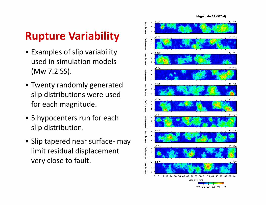
Rupture Variability
• Examples of slip variability
used in simulation models
(Mw 7.2 SS).
• Twenty randomly generated
slip distributions were used
for each magnitude.for each magnitude.
• 5 hypocenters run for each
slip distribution.
• Slip tapered near surface- may
limit residual displacement
very close to fault.
Residual Displacement
• Grows with increasing
magnitude.
• Generally decreases with
increasing distance except
very close to larger
magnitudes- slip taper(?).
• Variability increases with • Variability increases with
increasing magnitude.
• Variability decreases with
increasing distance.
• Pulse period lengthens as a function of increasing magnitude and distance
• Average pulse start time lengthens as a function of increasing magnitude
• Average pulse start time decreases as a function of increasing distance
(Mw > 7), and approaches the P-wave arrival time as a limiting (minimum)
value, consistent with elastic rebound theory.
• The key component in the numerical simulations is the
characterization of rupture.
• Residual displacement controlled by fault
displacement “near” the site.
• Pulse width controlled by rise-time, rupture velocity
and fault slip.and fault slip.
• Rupture generator methodologies have evolved since
time of initial fling simulations.
• Bykovtsev and Kramarovskii (1987 in Russian, 1988)
• Frankel (1991), Frankel (2009)
• Zeng, Anderson and Yu (1994)
• Guatteri, Mai and Beroza (2004)
Some Recently Proposed Kinematic
Rupture Generators:
• Guatteri, Mai and Beroza (2004)
• Graves and Pitarka (2004), Graves and Pitarka (2010)
• Liu, Archuleta and Hartzell (2006), Schmedes, Archuleta and
Lavallee (2010)
• Song and Somerville (2010)
• Aagaard, Graves, Schwartz, Ponce and Graymer (2010)
Currently available on SCEC Broadband Platform
Evolution of Rupture CharacterizationGraves and Pitarka 2004:
Weak timing perturbations
Graves and Pitarka 2010:
Strong timing perturbations
Significant reduction in
rupture coherence
Liu, Archuleta and Hartzell (2006)
• Slip distribution following Mai and
Beroza (2002) mapped to Cauchy
distribution
• Correlation between rupture velocity
and slip is set at 30%. Rupture velocity
has uniform distribution of 0.6 to 1.0 Vs
(average 80% Vs)
Correlated Random Source Parameters
(average 80% Vs)
• Correlation between rise time and slip
is set at 60%. Rise time has beta
distribution with τmin = 0.2 τmax and τmax
constrained to fit the high frequency
level of a Brune spectrum
Schmedes, Archuleta and Lavallee (2010)
• Extends Liu et al (2006) by utilizing
dynamic simulations to determine
correlations among kinematic parameters
• Slip function characterized by peak time
and rise time
• Rupture velocity not correlated with slip,
but has strong (negative) correlation with
Correlations inferred from Rupture Dynamics
but has strong (negative) correlation with
peak time
• Rise time has strong correlation with slip
• Are the existing numerical experiments still useful/relevant?
� Limited by outdated version of rupture characterization
• Should the design of these experiments be modified or
augmented to address additional issues?
� Magnitude range, station layout, rupture type?
• What are potential effects related to assumed Mag-Area
Discussion
• What are potential effects related to assumed Mag-Area
relation(s)?
• Should a completely new set of simulations be run (using
current methodologies)?
• Is the proposed “fling-pulse” model acceptable?
� Should additional parameters (beyond D, Tf, t1) be modeled?
• What about constraints from other simulation approaches, e.g.