LATE PLEISTOCENE GLACIAL HISTORY OF CENTRAL MARQUETTE AND NORTHERN DICKINSON COUNTIES, MICHIGAN By Robert S. Regis A DISSERTATION Submitted in partial fulfillment of the requirements for the degree of DOCTOR OF PHILOSOPHY (Geology) MICHIGAN TECHNOLOGICAL UNIVERSITY 1997
Transcript
LATE PLEISTOCENE GLACIAL HISTORY OF CENTRAL MARQUETTE ANDNORTHERN DICKINSON COUNTIES, MICHIGAN
By
Robert S. Regis
A DISSERTATION
Submitted in partial fulfillment of the requirements
for the degree of
DOCTOR OF PHILOSOPHY
(Geology)
MICHIGAN TECHNOLOGICAL UNIVERSITY
1997
This dissertation, "Late-Pleistocene Glacial History of Central Marquette and Northern
Dickinson Counties, Michigan", is hereby approved in partial fulfillment of the
requirements for the degree of DOCTOR OF PHILOSOPHY in the field of geology.
DEPARTMENT: Geological Engineerinjand Sciences
Thesis Advisor
HewroT Department
April 28, 1997Date
PREFACE
Glacial processes affected broad regions in the northern part of North America and
many parts of the world, yet in many areas, little is known about the details of glacier
movements. To better understand the glacial history of the central Upper Peninsula of
Michigan and to identify new techniques that will help improve interpretations of the
glacial history in any region, three related studies were conducted. The first study used
diverse digital datasets and computer image processing techniques in place of traditional
maps and aerial photographs for interpreting and mapping the spatial distribution of glacial
landscape features. The second study incorporated field and laboratory data with the
interpretations made in the first study to describe the movements of glacial ice within the
central Upper Peninsula. The third study explored a relationship between drumlin
orientation and form to underlying bedrock geology that was first recognized in the image
processing study.
In the first study, several diverse digital datasets were pre-processed so that they
could be easily combined. Image processing algorithms such as the Intensity-Hue-
Saturation (IHS) transformation were applied to the dataset combinations to test their
utility for interpreting and mapping glacial landforms. Digital elevation model (DEM),
Side-Looking Airborne Radar (SLAR), Thematic Mapper (TM), and several ancillary
datasets proved to be effective replacements for traditional interpretation tools such as
aerial photographs and topographic maps. From this study, it was concluded that digital
image processing of diverse datasets can be used to effectively analyze glacial landscapes
and in many cases, replace traditional interpretation tools.
The second study was undertaken to interpret the movements of glacial ice
through the central Upper Peninsula region utilizing information from the image
processing study combined with field and laboratory studies of sediments and geomorphic
features. The stratigraphy of geomorphic features identified in the image processing study
was examined and sediment samples were collected, and analyzed in the lab to determine
texture and lithology. From this study, it was interpreted that two ice lobes initially
advanced across the region and then retreated into the Lake Superior basin. In the
northern and northwestern parts of the study area, the Michigamme lobe moved forward
from the northeast. In the southeast and southern parts of the study area, the Green Bay
lobe moved initially toward the southwest, but refracted so that it finally moved in a
westward direction. After they retreated, the Superior lobe advanced and deposited a
large moraine and outwash plain that parallels the modern Lake Superior shoreline about
10 km inland. The lobe retreated into the Lake Superior basin and the ice never returned.
A compelling relationship between drumlin form and orientation with bedrock
geology is the subject of the third chapter. When Side-looking Airborne Radar (SLAR)
data was combined with a scanned geologic map, it was noted that characteristics of
drumlins change precisely at the contact between Ordovician limestone (east) and
Cambrian sandstone (west). Drumlins over limestone have mean length/width ratios of
6.0 and are oriented toward the south-west, those over sandstone have length/width ratios
of about 4.0 and are oriented toward the west. Variation in porewater pressure in the
subglacial sediments, which affected their shear strength, is thought to be responsible for
the differences.
Ill
ACKNOWLEDGMENTS
Most of all, I would like to thank my major advisor, Jackie Huntoon. Jackie led
me through my graduate tenure with grace. She always seemed to know when to give me
some words of encouragement. Even though the editing process must have been a real
chore at first, because of the poorly written text I imposed upon her, her commitment to
my success was always apparent. This dissertation was improved immeasurably by your
suggestions. I can't thank you enough.
I would also like to express thanks to Steve Shetron. Steve became a mentor and
friend early in my research. Thank you for the invigorating discussions, field trips, and for
your library. You always kept me "on my toes" by pointing out alternatives to my
explanations, which improved this dissertation greatly, and made a better researcher out of
me.
Ann Maclean deserves a lot of thanks for this dissertation because she helped to
improve my methodology for delineating glacial landforms. From the beginning of my
research, she provided me with an "open door" to her image processing lab, and to her
expertise. Because of that, my research was improved substantially. Thank you, Ann.
To the fourth member of my advisory committee, Bill Rose, thank you for listening
to, and for critical review of potential dissertation proposals, and for allowing me the
freedom to "march to my own drummer". Also, thank you for your support, especially in
the important first year of the program. I'm sure that you were instrumental in acquiring
most of my funding.
IV
I would also like to recognize others who helped me through the program. First of
all, I want to thank Neil Hutzler, who volunteered to serve on my written and oral
qualifying exam committees, and for helping me to sustain funding through the GEM
grant. Thank you John Gierke and Sue Beske-Diehl for volunteering to serve on my
written and oral qualifying exam committees, and to John Hughes for serving on my
written qualifying exam committee, for being a mentor and friend, and for inspiring me to
undertake the study of glacial geology.
A special thank you goes to Bonnie Gagnon, who sheltered me from institutional
bureaucracies and red tape, made sure my records were submitted in the right order, even
though they weren't always prepared in the right sequence, and generally made the
administrative chores less painful.
Thank you to all of the faculty in the Department of Geography, Earth Science,
Conservation, and Planning at Northern Michigan University, especially Pat Farrell and
Fred Joyal. Your support by hiring me before completing this dissertation was greatly
appreciated. Your support also got me through some rough times while trying to perform
my full-time job with many new classes, at the same time setting up and maintaining a new
computer lab, all the while trying to find time to complete this dissertation.
This project benefitted from intellectual discussions with many people during my
research. Thank you to faculty members Ted Bornhorst, Jimmy Diehl, Doug McDowell,
Bill Gregg, Chuck Young, and Alex Mayer, and to fellow graduate students Dave
Schneider and Drew Pilant. Thanks also to Bob McCarthy for help with laboratory work.
Last, but not least, thanks to my family. To my wife Monica, and to Brent and
Stephanie, who followed me to three different universities, sometimes with enough
resources to barely cover the moving expenses, we can finally look back on the rough
times, the good times, and see humor. I wouldn't trade them for anything. Finally, I want
to thank my parents, George and Becky, who instilled the perception that if I believed in
my own capabilities, success would surely follow. As usual, they were right.
VI
TABLE OF CONTENTS
Chapter 1: Use of DEM, SLAR, and TM Data for Interpreting and MappingGlacial Landscape Units, Central Upper Peninsula, Michigan.
ABSTRACT 2
INTRODUCTION 4
BACKGROUND 6Study Area 6Surface Geology 6
SYSTEM 8
DATA 9Digital Elevation Model (DEM) 9Thematic Mapper 11Side-Looking Airborne Radar 11Digital Geologic Map 12Other Digital Datasets 12
METHODOLOGY 13Digital Elevation Model Derivatives 13
DATA 64Topography 64Sediments 67Moraines, ice contact features, and outwash plains 73Interlobate deposits 85Proglacial lake landforms 89Ablation hills 93Drumlins 95Loess 96
TEMPORAL MOVEMENTS OF GLACIAL ICE 96Retreat from the late Sagola and Republic moraines 98Retreat from the Green Hills and Ishpeming positions 100Gribben Interstadial 102Gribben forest 103Marquette Stadial 112
CORRELATION 122
CONCLUSIONS 127
REFERENCES 130
vm
Chapter 3: Bedrock Control of Drumlin Morphology and Orientation
ABSTRACT 135
INTRODUCTION 137
STUDY AREA 143
METHODOLOGY 147
DRUMLIN MORPHOLOGY AND ORIENTATION 149Relationship to bedrock geology 149
STATISTICS 153
DRUMLIN SEDIMENTOLOGY AND STRATIGRAPHY 154
NON-DRUMLIN LANDFORMS 160Troughs between drumlins 160Transverse feature 163Outwash fan and tunnel channel 166
BEDROCK CONTROL ON WATER PRESSURE 169
DISCUSSION 179
CONCLUSIONS 182
REFERENCES 184
IX
LIST OF FIGURES
Chapter 1.
Egure1. Study area location and size 72. Methodology flowchart 233. IHS transformation (DEM, relief; east and north illumination) 254. IHS transformation (DEM, SLAR, PCI) 275. IHS transformation (PC 1, DEM, relief) 296. IHS transformation (geology, PCI, SLAR) 307. Perspective view, DEM with relief (westerly look direction) 338a. Classification image: 3-band 378b. Classification image: 4-band 388c. Classification image: 5-band 408d. Classification image: 8-band 41
Chapter 2.
Figure1. Study area location and size 522. Bedrock geology of the study area 613. Contour and perspective view maps of bedrock topography 624. Perspective view of surface topography 655. West-east surface profile across the study area 666. Textural triangle showing till samples 697. Ternary plot: percentage of lithologic components in till 708. Contour map showing distribution of lithologic components 729. Photo of sediment exposure: outwash sand over till 76lOa. Photo of sediment exposure: foliated till over outwash 77lOb. Close-up of from area just to right of Figure 10(a) 7911. Tributary (parallel) channels of the Escanaba River 8112. Green Hills topographic map (north part) 8613. Portion of the Cataract Basin topographic quadrangle 8814. Boulder train 9015. Green Hills topographic map (south part) 9216. Portion of the Sands topographic quadrangle 9417. Loess filling a small postglacial channel 9718. Interpretation of ice marginal positions 9919. Location and size of trees unearthed in the Gribben Basin in 1978 10520. Photo of in situ spruce tree unearthed in the Gribben pit 110
Chapter 2. (continued)
21 . Cross section showing sediments and standing trees 1 1 122. Location of the Gribben forest 1 1323. Locations and C14 dates of organic materials 1 1424. Ponding of water in front of advancing Marquette ice 11625. Maximum position of Marquette ice 11726. Position of ice while outer Marquette moraine formed 1 1 827. Position of ice while inner Marquette moraine formed 12028 . Map of Marquette moraines 1 2 129. Regional correlation of moraines 1 23
Plate
1 . Glacial landscape units in pocket
Chapter 3.
Figure1 . Drumlin formation resulting from rheological differences 1392. Impact of porewater pressure on subglacial sediments 1413. Study area 1444. Generalized bedrock geology 1455. Overburden thickness/geology/drumlin relationship 1486. SLAR/geologic map combined image 1507. An example of some drumlin forms 1 528. Photo of gravel pit exposing a drumlin interior 1 569. Close-up view to the right of Figure 8 1 5710. Drumlin interior exposure 1 591 1 . Topographic map (Northland, MI quadrangle) 1611 2. Photo of gravel pit 1 6213. Cross section of asymmetrical drumlins 1 6414. Cross section through transverse (to ice flow) feature 1651 5. Close-up of contorted strata 1 671 6. Landsat TM image 1 6817. SEFTRAN finite element numerical groundwater model output 1 78
XI
LIST OF TABLES
Chapter 1.
Table1. Data characteristics 102. Datasets and their information content 213. Maximum-likelihood classifier accuracy assessment 35
Use of DEM, SLAR, and TM Data for Interpreting and MappingGlacial Landscape Units, Central Upper Peninsula, Michigan
ABSTRACT
New techniques for mapping glacial landscape units located in the central Upper
Peninsula of Michigan were developed using image processing software. Digital Elevation
Model (DEM), Side-Looking Airborne Radar (SLAR), Landsat Thematic Mapper (TM)
and overburden thickness (OBT) datasets were used. Many combinations of the DEM,
SLAR, and TM datasets using the Intensity-Hue-Saturation (IHS) and Principal
Components Analysis (PCA) transformations were valuable for visual interpretation of
glacial landscape units. Such combinations showed relative elevations of landscape units,
relief variations, and surface cover types in a single image. Also in the study, relief images
and three-dimensional perspective views derived from the DEM were used to map ice-
marginal positions and interpret how glacial ice receded from the area. The stair-step
appearance of glacial outwash terraces at progressively lower elevations toward the east
became evident using the perspective view technique. Visualization of glaciated terrain
using these datasets in an image processor proved to be more effective for interpreting
glacial landscapes than traditional topographic map or aerial photograph analyses.
Texture analysis of the DEM was used to provide a measure of terrain ruggedness
(or roughness) as input to a supervised maximum likelihood classification algorithm.
Standard deviation of the DEM was assessed as a measure of texture in four moving
windows of the following sizes; 64 pixels2, 32 pixels2, 16 pixels2, and 3 pixels2. Windows
of different sizes were used to match the frequency of natural variation in size and spacing
of features that comprise each of the landscape units in the study area. Texture files were
combined with the TM, DEM, and OBT datasets into a single multi-band file. The
3
maximum likelihood classification algorithm was then applied to the multiple-dataset file.
The algorithm was first applied only to the two principal components (PCI and PC2) of
the TM's six non-thermal bands, then each remaining dataset was added, one at a time, and
the algorithm was re-applied until all eight datasets (PCI, PC2, DEM, OBT, and the four
texture datasets) were used. When compared to ground truth data, classification accuracy
utilizing all eight datasets reached a maximum of 68.6% correctly classified pixels.
Without any textural measure included in the classification (only using PC's, DEM, and
OBT), overall accuracy was 54.2%. The addition of each dataset significantly improved
the overall performance, suggesting that when classifying glacial landscape units, land
cover, topography, overburden thickness, and a measure of surface roughness improves
the accuracy of glacial landscape classification.
INTRODUCTION
Identification and classification of landscapes is based on the premise that areas of
the earth's surface may be characterized by a unique set of internally homogeneous
properties such as slope, form, hydrologic characteristics, etc. (Townshend, 1981). Such
areas are composed of assemblages of feature types that collectively form a landscape unit.
In the heavily-wooded, glaciated Superior Upland province of North America, landscape
units are mapped via relief, topographic form of individual features, associations of
multiple features, vegetation patterns, and distribution of soils.
Topographic maps and stereoscopic aerial photographs are traditionally the
primary sources of information for geologists and physical geographers who interpret and
map glacial landscapes. These types of data provide researchers with inexpensive, readily
accessible spatial (X,Y and Z) information for interpretation and feature identification.
However, there are some problems associated with using these media types. To interpret
topographic maps, isolines of elevation on the map must be mentally converted to a three-
dimensional image of the terrain. The visualization and interpretation of earth surface
features made from isolines is a subjective process that is often associated with error,
particularly if the analyst is not highly trained. Aerial photographs, when used for
mapping land use/cover, also present interpretation problems since they are often acquired
"leaf-on". The vegetation masks subtleties of geomorphic form, making accurate landform
interpretation difficult. Another problem specific to interpreting glacial landscapes with
each of these tools is that much of the geomorphic detail is lost as the scale of the map
and/or photograph becomes smaller.
In contrast to topographic maps and aerial photographs, a computer-assisted
image processing system provides the hardware and software necessary for improved
visualization and analysis of geomorphic terrains when used with digital data. Image
processing and geographic information system (CIS) techniques may be used to
manipulate large digital datasets and to improve interpretability of the data. The
computer-assisted approach reduces interpreter subjectivity and biases inherent in
interpretations of topographic maps and aerial photographs. However, to adequately
characterize a glacial landscape using image processing techniques, the selection of proper
datasets, and the selection of appropriate processing algorithms are critical.
In a geomorphological context, many studies have shown that landforms can be
identified through the surrogate of vegetation using spectral data alone (Siegal and Goetz,
1977; Mussakowski et al., 1991). However, interpretation or classification of geomorphic
landscape units based solely on satellite spectral imagery is inadequate because not all of
the features comprising the whole unit (relative elevation and relief, for example) are
expressed. It is necessary to incorporate geomorphic and topographic parameters with the
satellite imagery to accurately map the landscape units. Digital Elevation Model (DEM)
and Side-Looking Airborne Radar (SLAR) data provide topographic and/or relief
information about surface features at a spatial resolution required for discrimination of
small landforms. Additionally, these datasets cover a sufficiently large surface area
necessary to characterize glacial landscape units.
BACKGROUND
Study Area
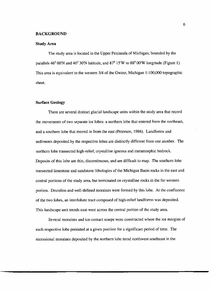
The study area is located in the Upper Peninsula of Michigan, bounded by the
parallels 46° OO'N and 46° 30'N latitude, and 87° 15'W to 88° OO'W longitude (Figure 1).
This area is equivalent to the western 3/4 of the Gwinn, Michigan 1:100,000 topographic
sheet.
Surface Geology
There are several distinct glacial landscape units within the study area that record
the movements of two separate ice lobes: a northern lobe that entered from the northeast,
and a southern lobe that moved in from the east (Peterson, 1986). Landforms and
sediments deposited by the respective lobes are distinctly different from one another. The
northern lobe transected high-relief, crystalline igneous and metamorphic bedrock.
Deposits of this lobe are thin, discontinuous, and are difficult to map. The southern lobe
transected limestone and sandstone lithologies of the Michigan Basin rocks in the east and
central portions of the study area, but terminated on crystalline rocks in the far western
portion. Drumlins and well-defined moraines were formed by this lobe. At the confluence
of the two lobes, an interlobate tract composed of high-relief landforms was deposited.
This landscape unit trends east-west across the central portion of the study area.
Several moraines and ice-contact scarps were constructed where the ice margins of
each respective lobe persisted at a given position for a significant period of time. The
recessional moraines deposited by the northern lobe trend northwest-southeast in the
UPPER PENINSULA
DF MICHIGAN
BEDROCKOUTCROPS
DRUMLINSAND FLUTES
ICE LDBEMOVEMENTS
MORAINES ANDICE-CONTACT SCARPS
DUTWASH PLAINS
STUDY AREA WITHGLACIAL FEATURES
L A K E S U P E R I O R
Figure 1. Study area. The study area comprises about 3300 sq. km in the central Upper Peninsula of Michigan.Features near KI Sawyer (KIS) Air Force base are younger than those to the west.
northern part of the study area. They become discontinuous between the bedrock knobs
prevalent in that region. In the southern half of the area, recessional moraines deposited
by the southern lobe trend approximately north-south and are curvilinear (concave toward
the east). Successively younger recessional moraines of both lobes occupy lower
topographic positions because the regional slope is toward the north and east in the
direction of ice margin retreat. Low-relief, large outwash plains accumulated beyond the
margins of each moraine. Continuous outwash plains join pairs of time-equivalent
moraines, one formed by each of the ice lobes, suggesting both lobes retreated uniformly
from the area. The moraine-outwash plain combinations form a distinct "stairstep" pattern
decreasing in elevation toward the north and east. Additionally, a single lobe deposited a
final, large moraine-outwash plain combination is found in the extreme northeastern
portion of the study area (Figure 1).
SYSTEM
An IBM compatible personal computer supporting Earth Resources Data Analysis
System (ERDAS®) software was the main system used in the analysis. The system
included a 48 x 36 inch (active-area) digitizer, an Eikonics digital color scanner (4096
pixels2), and a high-resolution (1024 pixels2) 24-bit color monitor. The ERDAS software
is a raster-based application that has the capability of both image processing and GIS
functions.
DATA
Several commercially available digital datasets and photo-products were used in
the study. Their characteristics are described below and are summarized in Table 1.
Additionally, a digital geologic dataset was created from a scanned analog geologic map,
and an overburden thickness dataset was constructed from water-well drilling records,
geophysical, and bedrock outcrop data.
Digital Elevation Model (DEM)
The west half of the Marquette, Michigan 3-arcsecond DEM was used in this
study. It is a level 3 product of the USGS. Each pixel of the data in its raw form
represents about 80 m2 of ground area. Absolute elevation accuracy of these data is Vz the
contour interval (50 feet) of the parent topographic map product at a 90% confidence
level (U.S.G.S., 1987). For this study, it equates to nominal elevation accuracy of
approximately ±8 m. Relative elevation accuracies within a region, however, are generally
much better (U.S.G.S., 1987). This is advantageous for the present study because
absolute elevation is not as important as changes in elevation (relief) for identification of
glacial landscapes.
10
Table 1. Data and characteristics.
DATA TYPE
Digital Data
DEM
SLAR (Aeroservice)
SOURCE
U.S. Geological Survey
U.S. Geological Survey
LANDS AT TM EOSAT Corp.
Photo Products
SLAR U.S. Geological Survey
LANDSAT TM EOSAT Corp.
CHARACTERISTICS
1:250,000 (3-arcsecond)approx. 80x78 m pixelsMarquette, MI (west Vi)
X-Band (2.5 cm wavelength)HH polarizationSouth lookFar rangeapprox. 10m2 pixelsAcquisition date 6-88
(X,Y, and thickness) were entered into a spreadsheet software program, exported into a
software package (Surfer) and kriged to produce a regularly-spaced grid of output values
(dimensions = 500 lines by 500 columns) to encompass the entire study area. Finally, the
data were converted to ERDAS image format. The data were then resampled using the
cubic convolution spatial interpolation technique before incorporation into classification
and enhancement procedures. The dataset that resulted from this procedure is a
generalization of overburden thickness, because the distribution of data points across the
study area was non-uniform. However, it is thought to be an acceptable representation of
overburden thickness conditions because in this study, glacial landscape units are defined
13
by only a few thickness classes (for example, "thin overburden" of 0-10 m, "moderate
thickness" of 10-20m, and "thick overburden" of >20 m).
METHODOLOGY
Digital Elevation Model Derivatives
Texture images
Textural analysis was performed to assess variations in spatial homogeneity of the
DEM. Texture is defined as "virtually any type of spatial variation" (Townshend, 1981).
With textural analysis, a movable window centers on each pixel and a user-defined
mathematical function is applied to the digital numbers (DN's) of all the pixels within the
window. The size of the window (specified in units of number of pixels but equated to
ground units, or distance) assessed at one time is also selected by the analyst. Various
algorithms may be applied within the window as measures of texture, such as minimum-
maximum difference or standard deviation of the elevation values.
The derivation of textural information from digital datasets has been shown to
greatly improve classification performance when using a DEM or spectral data such as
Landsat Multispectral Scanner (MSS, which has 4 bands of spectral data). Franklin
(1987) reported improvement in classification of subarctic landscapes by adding five
geomorphic derivatives (elevation, convexity, relief, slope, and incidence) of a DEM to
MSS data. When using MSS data alone for nine landscape classes, overall accuracy was
46%. However, when the DEM data and its derivatives were added to the spectral data,
classification accuracy rose to 75%. In a similar study, applied explicitly to a DEM,
14
Franklin and Peddle (1987) presented a C-language program for textural analysis, and
applied it to a DEM of a mountainous region in Canada. They concluded that texture
information provides an independent measure of surfaces, and can be interpreted alone.
Franklin (1989), continuing his work on terrain analysis via image processor,
demonstrated that classification accuracy for land systems mapping improved from 40%
using only MSS data to 85%, simply by including elevation and slope data derived from a
DEM. Shih and Schowengerdt (1983), in a study of terrain units in Arizona, showed that
texture measures were extremely valuable for classifying geologic/geomorphic surfaces.
However, they only used Landsat MSS data as the source for texture analysis.
Hutchinson (1982) summarized the advantages and disadvantages of several methods for
combining spectral (MSS) and ancillary datasets. For natural resource applications, the
author suggested the use of ancillary datasets with computer-assisted classification
techniques holds "much promise". However, in contrast to most other studies, he
stipulates that "the simple addition of new observations increases computer time and does
not appear to improve classification accuracy with any consistency" (p. 128). As
microprocessor speeds increase, computer time required for classification of large, multi-
band datasets becomes less of an issue. Classification accuracies are, however, heavily
weighted by the quality of training samples selected to represent the classes involved, and
the spectral and ancillary datasets selected for the study at hand. Weszka et al. (1976)
cited a 90% classification accuracy of geologic features using only the textural derivatives
from a series of scanned black & white air photos. The authors compared three
approaches to derive textural information from the photos (Fourier transform, second-
15
order grey-level statistics, and first order grey-level statistics). In general, the Fourier
transform performed poorly. The reason cited was that terrain characteristics are usually
not periodic. Second and first-order grey-level statistics were found to perform well. In
fact, the simpler, first-order statistics such as standard deviation, consistently out-
performed more complex second-order statistics, such as convexity. Evans (1972, p.31),
in a discussion of statistical methods for measuring geomorphometry, states that "it is
logical that relief...should be measured by the standard deviation of altitude".
Standard deviation (S.D.) of the DEM was used to measure terrain ruggedness
(relief) in the present study. Standard deviation has been shown to be an effective
measure of relief, but using only one window size (corresponding to a finite area on the
ground) emphasizes landscape features that are about the same size as the window. For
example, a window designed to emphasize outwash plains would not be useful for
delineating a drumlin field because individual drumlins are much smaller than an outwash
plain. The use of several different areas of coverage for a complete relief analysis within a
region have been suggested in the literature, but not specifically for use in the image
processing context. Trewartha and Smith (1941), for example, suggested that the size, or
area of coverage, should be adjusted to match areas of different topographic frequency. In
a similar manner, Clark and Boulton (1989) showed how multi-scale remote sensor
datasets were necessary to match the frequency of natural variation of surface glacial
features and that a single dataset would be insufficient. In this study, four different
window sizes were applied to the DEM dataset to measure texture of the land surface
(relief). The size of the windows were designed to match the frequency and size of natural
16
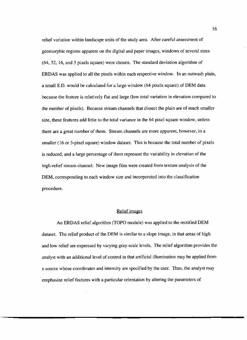
relief variation within landscape units of the study area. After careful assessment of
geomorphic regions apparent on the digital and paper images, windows of several sizes
(64, 32, 16, and 3 pixels square) were chosen. The standard deviation algorithm of
ERDAS was applied to all the pixels within each respective window. In an outwash plain,
a small S.D. would be calculated for a large window (64 pixels square) of DEM data
because the feature is relatively flat and large (low total variation in elevation compared to
the number of pixels). Because stream channels that dissect the plain are of much smaller
size, these features add little to the total variance in the 64 pixel square window, unless
there are a great number of them. Stream channels are more apparent, however, in a
smaller (16 or 3-pixel square) window dataset. This is because the total number of pixels
is reduced, and a large percentage of them represent the variability in elevation of the
high-relief stream channel. New image files were created from texture analysis of the
DEM, corresponding to each window size and incorporated into the classification
procedure.
Relief images
An ERDAS relief algorithm (TOPO module) was applied to the rectified DEM
dataset. The relief product of the DEM is similar to a slope image, in that areas of high
and low relief are expressed by varying gray-scale levels. The relief algorithm provides the
analyst with an additional level of control in that artificial illumination may be applied from
a source whose coordinates and intensity are specified by the user. Thus, the analyst may
emphasize relief features with a particular orientation by altering the parameters of
17
illumination. In the present study, low-altitude illumination from east and north azimuths
were used because the regional slope is toward the northeast. East and north-facing
slopes (such as moraines and ice contact scarps) were brightly illuminated using these
parameters, while outwash plains (that slope toward the west) were darker-toned.
Perspective Views
Perspective views of digital datasets aid interpretations by allowing visualization of
relative spatial changes in Z-values across a surface. Perspective views that are created
from a DEM are a manifestation of the terrain. When a relief image is "draped" over a
perspective view, variations in tone that correspond to degree of slope further enhance the
separation between low-elevation and high-elevation areas.
Perspective views eliminate many problems inherent in other methods of
geomorphic interpretation. Data are displayed in a form that the analyst can easily
perceive, with geomorphic features emphasized by variations in grey-scale tones. Thus,
the investigator can spend more time analyzing the image, and less time converting
information from another format such as topographic maps. In the present study,
perspective views of the DEM were used to analyze the spatial associations (relative
elevations and relief) between moraines and outwash plains, interlobate regions, bedrock-
controlled topography regions, and reconstruction of dissected outwash plains.
18
Thematic Mapper Derivatives
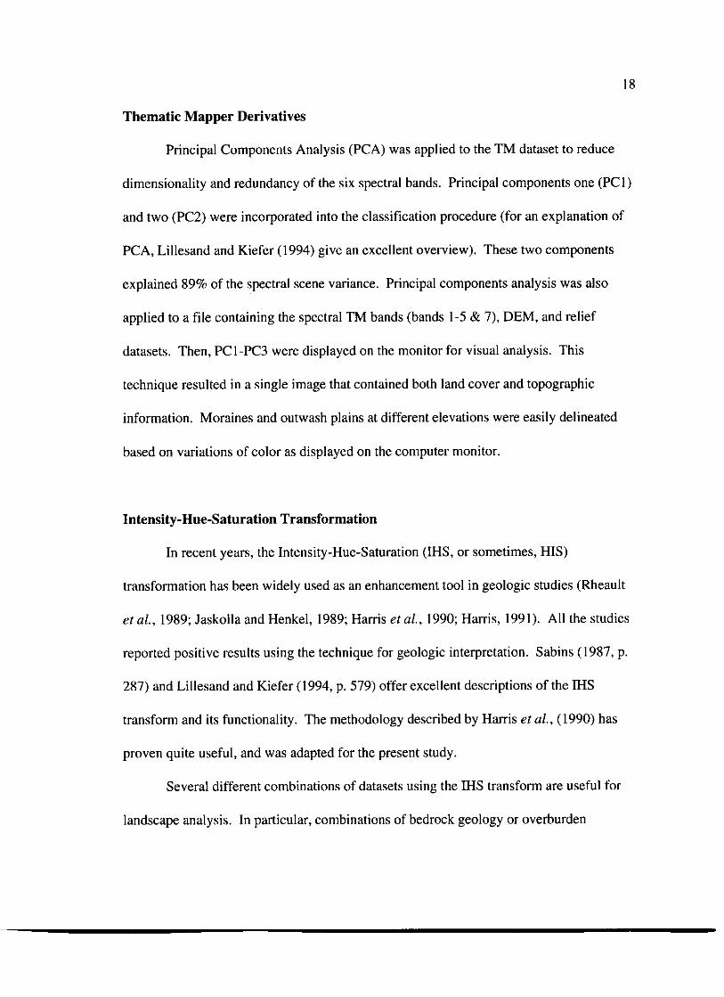
Principal Components Analysis (PCA) was applied to the TM dataset to reduce
dimensionality and redundancy of the six spectral bands. Principal components one (PCI)
and two (PC2) were incorporated into the classification procedure (for an explanation of
PCA, Lillesand and Kiefer (1994) give an excellent overview). These two components
explained 89% of the spectral scene variance. Principal components analysis was also
applied to a file containing the spectral TM bands (bands 1-5 & 7), DEM, and relief
datasets. Then, PC 1-PC3 were displayed on the monitor for visual analysis. This
technique resulted in a single image that contained both land cover and topographic
information. Moraines and outwash plains at different elevations were easily delineated
based on variations of color as displayed on the computer monitor.
Intensity-Hue-Saturation Transformation
In recent years, the In tensity-Hue-Saturation (IHS, or sometimes, HIS)
transformation has been widely used as an enhancement tool in geologic studies (Rheault
etal., 1989; Jaskolla and Henkel, 1989; Harris et «/., 1990; Harris, 1991). All the studies
reported positive results using the technique for geologic interpretation. Sabins (1987, p.
287) and Lillesand and Kiefer (1994, p. 579) offer excellent descriptions of the IHS
transform and its functionality. The methodology described by Harris et a/., (1990) has
proven quite useful, and was adapted for the present study.
Several different combinations of datasets using the IHS transform are useful for
landscape analysis. In particular, combinations of bedrock geology or overburden
19
thickness with SLAR and TM datasets clearly shows relationships that would otherwise
not be apparent. Also, IMS combinations of DEM with relief images provided valuable
information for reconstructing outwash plains that formed contemporaneously but are now
dissected by stream valleys. Combinations of the DEM and SLAR with TM through the
IHS transformation expressed topographic information the TM does not provide, allowing
more accurate interpretation of moraines, outwash plains, and drumlinized terrain.
Additional Image Transformations
Simple algebraic manipulations of SLAR and TM datasets are quite useful for
enhancing geomorphic forms and aiding interpretations. For example, one of the most
useful enhancements for studying the drumlin landscape found in the southeast quadrant of
the study area was multiplication of the single SLAR dataset with three separate TM
bands (7,5,4 or 5,4,3 in R,G,B) to produce an enhanced color-composite image.
Mussakowski et at. (1991) reported similar findings. This technique preserves the original
spectral information of the TM data, but the benefits of the SLAR data (relief information)
are incorporated. Distribution of surface features, such as vegetative associations, rivers,
and lakes are clearly apparent in the TM data, but not easily perceived by viewing the
SLAR data alone. The data mutually compliment each other.
The application of edge-enhancing filters improved the visual appearance and
information content of nearly all datasets. DEM and TM datasets were improved by
passing a 5x5 non-directional edge-enhancing filter over them. The SLAR data, which has
a very high spatial frequency, was improved by first applying a 5x5 high-pass filter to
20
further increase the spatial frequency, and then applying a 3x3 low-pass filter to smooth
the dataset. The procedure retains the general spatial variations in the SLAR data that
correspond to landforms, but smooths the dataset by decreasing the high spatial contrast
between adjacent pixels.
Classification
The "logical channel" approach (Strahler et al., 1978), also called the
"probabalistic method" (Franklin, 1989), of classification was used in this study. This
involves the simple addition of ancillary data (in the present study, DEM, texture
measures, and overburden thickness) to spectral (TM) data in a statistical classification
procedure. A maximum likelihood (Mahalanobis) supervised classification algorithm was
applied to a file containing the eight datasets in Table 2. These datasets were chosen
because each represents a unique component of glacial landscape units. For example, the
DEM data was used to delineate outwash plains and moraines at different elevations.
Textural measures aided separation of landscape units with differing topographic
frequencies. Principal components added spectral response information
for separability based mainly on vegetation changes. The overburden thickness
information helped the classifier to differentiate between moraine (thick deposits of
sediment) and thin drift classes (such as thin drift over bedrock). Both of these classes
21
Table 2. Datasets and their information content for analyzing GLU's.
DATASET INFORMATION CONTENT
1)DEM2) Texture (642 pixel SD of DEM)3) Texture (322 pixel SD of DEM)4) Texture (162 pixel SD of DEM)5) Texture (32 pixel SD of DEM)6) Overburden Thickness7)TMPC18) TM PC2
Elevation and reliefLarge-area relief variationsMedium-area relief variationsMedium-area relief variationsSmall-area relief variationsThickness of sediment depositsLand cover typesLand cover types not in (7).
have similar relief characteristics, are located at comparable elevations, and have similar
land cover types.
Eleven distinctly different geomorphic units (classes) were identified through use
of the hard copy TM product and SLAR, topographic maps, and field reconnaissance. At
least three characteristic areas of each class were identified and digitized into polygons and
saved as training areas. Statistics were extracted for use in the classification algorithm.
The maximum likelihood classification algorithm was systematically applied to
various combinations of the datasets to assess their utility in classification of glacial
landscape units. Using the work of Franklin (1987, 1989) and Franklin etal. (1987) as a
guide, many combinations were tried and assessed visually before a standardized
procedure was established. First, only the principal components pair of datasets (TM PC 1
and PC2) were classified by extracting statistics from training area polygons in those two
"bands", then applying the classification algorithm to those "bands" only. The resulting
file was identified by the name "2-Band". Training area polygons were then applied to
22
PCI and PC2 with the DEM added (3-Band). Statistics were extracted and the scene was
classified. The same procedure was applied to combinations of PCI, PC2, DEM with
OBT added (4-Band), with PCI, PC2, DEM, OBT, and the 64 pixel2 S.D. textural
measure added (5-Band). The procedure was continued by adding individual texture
datasets until finally, the area was classified using the entire, eight-band dataset (8-Band).
A single accuracy assessment table was produced for evaluation of all classified
scenes. Five hundred (software maximum) stratified random pixels (software-selected)
were displayed on the monitor. Interactively, with "ground truth" such as topographic
maps and aerial photographs, and with field verification, "correct" classes were assigned to
each reference pixel. Accuracy of each classified scene using the different band
combinations was assessed through comparison of the reference and classified pixels.
A flowchart (Figure 2) shows the procedure for analysis of the datasets. All data
were registered to a common geographic coordinate system (Universal Transverse
Mercator, UTM), bounding coordinates, and pixel size. This allowed combinations and
interactions between the datasets to be performed freely. The DEM, TM, and overburden
thickness data were rectified and resampled to 56x54 m2 per pixel as a compromise
between the coarse resolution of the DEM and the finer resolution of the other datasets,
and so the entire (non-square) study area could be displayed on the 10242 pixel resolution
monitor without reduction. For more detailed analysis in specific areas, the TM and
SLAR datasets were rectified and resampled to 28.5 m2. The DEM dataset was not used
in those analyses.
PERSPECTIVEVIEWS
!HSTRANSFORM
GEOLOGIC MAP
CLASSIFICATIONACCURACY
ASSESSMENT
Figure 2. Methodology flowchart. Datasets used as input are enclosed in ellipses, functions performed on those data setsare within the small rectangular boxes (GCP = ground control points), outputs are in large rectangular boxes. The mainoutputs were perspective view images, images from the IHS transformation, and classified images.
to
24
IDENTIFICATION OF GLACIAL LANDSCAPE UNITS
In particular, the DEM dataset and its derivatives proved extremely valuable for
analyzing glacial geomorphic features and landscape units. The prime determinant of any
geomorphic form is spatial change in elevation (relief), justifying the use of DEM. The
raw DEM is useful by itself for initial landscape characterization, but is most useful after
application of a high-pass (edge-enhancing) filter. A filtered IMS transform combination
of DEM and relief images (east and north-illumination) emphasizes the assets of both. An
example of the IHS combination is shown in Figure 3; absolute elevation is portrayed as
gray-scale tones, with lower elevations as dark tones, high elevations in light tones. High-
relief features appear relatively bright because they are displayed in both the intensity
(north-illumination relief image) and saturation (east-illumination relief image) bands.
Outwash plains and other low-slope areas are represented by uniform-toned areas on the
image.
Most outwash plains at their respective elevation are bounded on the southeast and
northeast by linear, high-relief features. These are moraines and ice-contact scarps that
are expressions of the ice margin position at the time the corresponding outwash plain was
being constructed. The occurrence and spatial relationships of these features are evidence
that two ice lobes entered the area, one from the northeast, the other from the east, as
previously suggested by Peterson (1986). Continuous outwash plains bounded by the
moraine pairs indicate that two separate lobes were in place simultaneously, both
contributing to the formation of the plain.
25
46'30'
46°00'87*15'
54321O 5 10Kilometers
Figure 3. IHS transformation applied to DEM and relief datasets.
26
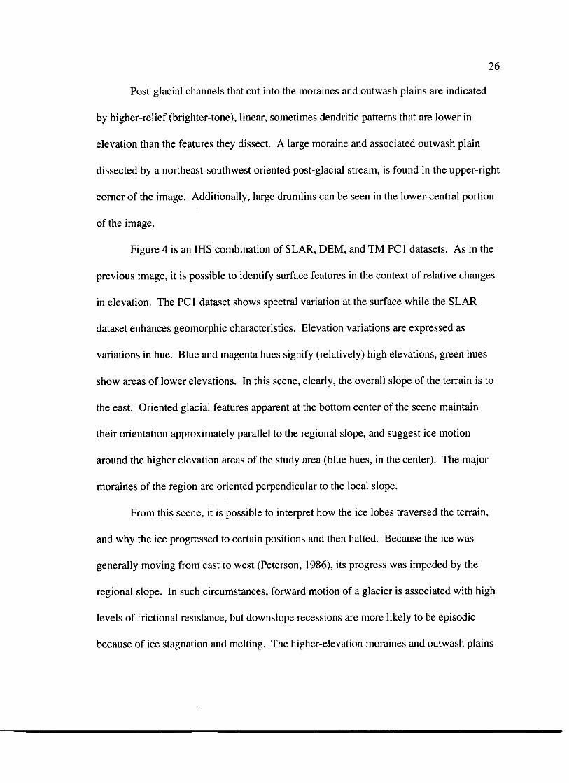
Post-glacial channels that cut into the moraines and outwash plains are indicated
by higher-relief (brighter-tone), linear, sometimes dendritic patterns that are lower in
elevation than the features they dissect. A large moraine and associated outwash plain
dissected by a northeast-southwest oriented post-glacial stream, is found in the upper-right
corner of the image. Additionally, large drumlins can be seen in the lower-central portion
of the image.
Figure 4 is an IHS combination of SLAR, DEM, and TM PCI datasets. As in the
previous image, it is possible to identify surface features in the context of relative changes
in elevation. The PCI dataset shows spectral variation at the surface while the SLAR
dataset enhances geomorphic characteristics. Elevation variations are expressed as
variations in hue. Blue and magenta hues signify (relatively) high elevations, green hues
show areas of lower elevations. In this scene, clearly, the overall slope of the terrain is to
the east. Oriented glacial features apparent at the bottom center of the scene maintain
their orientation approximately parallel to the regional slope, and suggest ice motion
around the higher elevation areas of the study area (blue hues, in the center). The major
moraines of the region are oriented perpendicular to the local slope.
From this scene, it is possible to interpret how the ice lobes traversed the terrain,
and why the ice progressed to certain positions and then halted. Because the ice was
generally moving from east to west (Peterson, 1986), its progress was impeded by the
regional slope. In such circumstances, forward motion of a glacier is associated with high
levels of frictional resistance, but downslope recessions are more likely to be episodic
because of ice stagnation and melting. The higher-elevation moraines and outwash plains
27
46'30'
88=00'
5 4 3 2 1 OMiles 10
543210 5 10Kilometers
15
N
Figure 4. IHS transformation of SLAR, DEM and TM PCI datasets.
28
in the west are evidence of earlier, more vigorous advances spared destruction by later
advances, or burial by sedimentation during retreat, because of the sloping terrain.
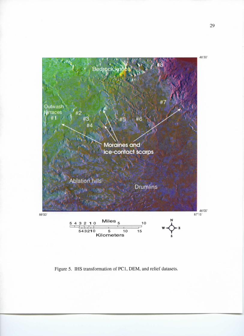
Combining the DEM and relief images with PCI provides the user with relief,
elevation, and spectral information. In Figure 5, an IHS transformation of PCI, DEM,
and relief, not only are relief features and absolute elevation apparent, as in Figure 4, but
the spatial relationships between surface land cover types and relief and elevation are
evident. The analyst can distinguish relationships between the distribution of deciduous
vegetation (brighter tones) and high relief (therefore usually drier) glacial features.
Likewise, poorly drained areas support moisture-tolerant species (spruce, cedar, etc.) and
are dark-toned on the image. Red and Jack pine dominate on outwash plains and appear
as an intermediate tone. The utility of using vegetation as a surrogate to surface geologic
and soils mapping has long been recognized (Tomlinson and Brown, 1962; Siegal and
Goetz, 1977). The combination of these datasets provides the capability of viewing
several different types of information at once. Thus, a more accurate interpretation may
result. For instance, in the right-center portion of the image is an interlobate tract of high-
relief ice-contact deposits. That feature is separable, in terms of relief, elevation, and
vegetation, from the terrain to the north or south. Also, stagnant-ice features in the
southwestern part of the study area (lower left) are clearly high-relief, deciduous-
supporting features.
Figure 6 shows another application of diverse data combination through use of the
IHS transformation. In this image, the scanned geologic map is represented by variations
in hue, consistent with the colors of bedrock lithologic units as portrayed on the original
,f I
Bedrock
Outwash 'terraces
1 #1 ;,'« SI #3
i^
Moraines and *'tee-contact Scarps
Ablation hillsDrumiins
88"00'
5 4 3 2 1 O MileS
54321O 5 1OKilometers
10N
15w-O-
46'00'87°15'
Figure 5. IHS transformation of PCI, DEM, and relief datasets.
Cambrian
30
. 46°30'
Mefasedtmenis
88°00'
r 1 r i i5 4 3 2 1 0 MHeS 5
543210 5 10Kilometers
10
15
OrdovicianLimestone
Dfumlins46W
87° 15'
N
Figure 6. IHS transformation applied to geology, TM PCI, and SLAR datasets.
31
map. The intensity and saturation components are represented by PCI and SLAR. The
original values of PC1 are retained, while relationships between the surface features and
bedrock geology become apparent. The orientation of drumlins (the small, linear forms in
the south-central part of the image) change from southwest/northeast in the eastern half of
the study area to northwest/southeast in the western half. The change in orientation
occurs over the contact between Ordovician limestone and Cambrian sandstone bedrock
lithologies (indicated by hue change). This is significant in that spatial variations in
bedrock geology are expressed through surface morphology. Drumlins are subglacially
formed features oriented in the direction of ice motion. Apparently, the bedrock geology
may have played a role in the formative processes of the drumlins. For field geologists,
exploration geologists, and geomorphologists, this finding is encouraging. Once more is
known about the processes of subglacial bedform construction and specifically, the effect
bedrock may have on their formation, remote sensing techniques may aid in mapping of
bedrock geology in glaciated terrain where other types of data are scarce. Although this
technique has been applied in an analog fashion in the past (map overlays), it is doubtful
that the data would show this relationship as clearly. Also, problems with the analog
method, such as combining maps of different scale, are less of an issue when using digital
image processing.
Perspective views
The combination of DEM with relief through the 3-D, or perspective view
functions of the image processor provide yet another way to perceive and analyze glacial
32
landscape units. Figure 7 is a perspective image of the DEM overlain by an east-
illumination relief image. The view direction is from south-southeast toward the north-
northwest. Through this function, terrain is represented in a visually familiar way. Mental
conversions are not necessary to perceive elevation changes, or relationships between
features. The outwash plains described previously are apparent at several, successively
lower elevations on this image. In this image, at least six separate levels are recognized,
indicating six or more separate stillstands (or minor re-advances) of the ice fronts.
Because the outwash plains at each level are continuous across the deposits of both ice
lobes, they are interpreted to have formed contemporaneously. In order for the glaciers to
construct outwash plains of this extent, it is interpreted that the ice must have persisted at
their respective positions for a significant period of time. The series of stair-stepped
outwash plains is also meaningful, as it records the recession of the ice masses
northeastward into the Lake Superior basin. Thus, it is interpreted that the recession of
glacier ice from the region was not uniform, and the intervals between adjustment to a
new equilibrium position are noteworthy.
Valleys of streams flowing eastward, that are currently dissecting the outwash
plains and moraines, are displayed as bright areas typical of rugged topography. In many
areas these stream valleys dissect the outwash plain to the extent that only separated,
remnant terraces remain. The perspective images are very useful in reconstructing the
former extent of outwash plains from isolated outwash terraces. On topographic maps or
aerial photographs, it is extremely difficult to mentally visualize these features. Most
often, only a portion of one remnant terrace may be found on a single topographic map.
Figure 7. Perspective view, DEM with relief (westerly look direction). Note the terraces at progressively lower elevationstoward the east (toward the viewer). Terrace numbers are described in the text.
34
Reconstruction of the entire terrace from isolated bits of information requires a good deal
of experience and imagination. On the computer image, however, the relationships
between disjointed terraces become very apparent.
Also on Figure 7, large hills are seen at a position where the two ice lobes met
(right-central part of the image, called the Green Hills on local topographic maps). They
formed where runoff of supraglacial meltwater was concentrated. These are ice-contact
interlobate deposits and comprise a distinct glacial landscape unit (based on relief and
spatial association).
Classification
Classification procedures applied to the datasets proved useful for automatically
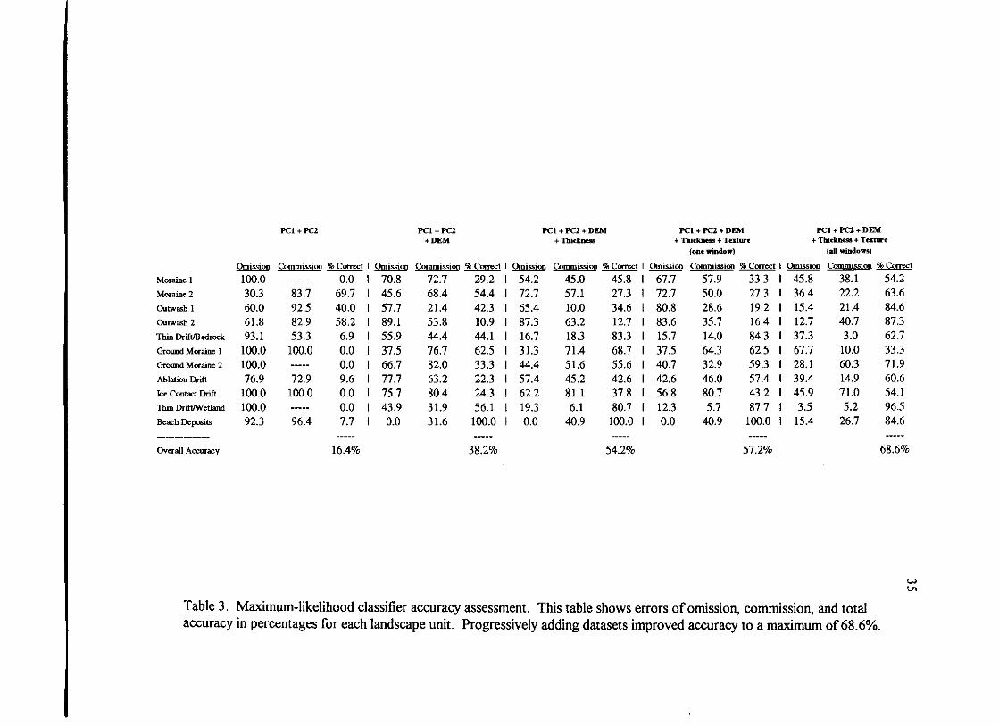
mapping glacial landscapes. Table 3 provides a classification summary for each class and
combination of datasets. The maximum likelihood classifier yielded only 16.4% accuracy
in errors of omission (pixels that should have been included in a category but were
omitted) using only PCI and PC2 (identified as "2-Band"). Errors of commission and
percent correct, also shown in Table 3, are those associated with pixels that were
improperly included in a class (Lillesand and Kiefer, 1994). The moraine/outwash plain
separability was adequate using "2-Band", probably because those features support
completely different vegetation. When PCI, PC2, and DEM was used, classification
accuracy rose to 38.2% ("3-Band"). Significant improvements were realized in the
identification of all landscape unit classes except the moraine and outwash classes. These
became worse because of confusion with other classes (for example, pixels that should
Table 3. Maximum-likelihood classifier accuracy assessment. This table shows errors of omission, commission, and totalaccuracy in percentages for each landscape unit. Progressively adding datasets improved accuracy to a maximum of 68.6%.
36
have been classified as moraine, but were classified as something else). When overburden
thickness was added ("4-Band"), classification accuracy increased 16%, to 54.2%. The
two "thin drift" classes gained most from the addition of this dataset. A slight
improvement in overall accuracy (54-58%) was realized by the addition of any one
textural dataset (the greatest improvement using a single textural measure was gained by
using the 64 pixel2 window dataset; "5-Band"). In fact, accuracy decreased in some
classes due to errors of omission. When all datasets were classified ("8-Band"), the
overall accuracy level in classifying glacial landscapes escalated to 68.6%. The most
significant gains were realized in the outwash and moraine classes, where errors of
omission were reduced by as much as 70%. One class, ground moraine 1, actually fell
significantly with the addition of the textural measures. The classifier confused pixels with
the similar, and spatially adjacent, ground moraine 2.
Figure 8 (a-d) shows the classified images "3-Band", "4-band", "5-band", and "8-
Band" for the entire study area. The classified images "2-Band", "6-Band", and "7-Band"
have little additional value, and are omitted. Color-coding of the classes is indicated by
the legend, and is consistent for all the images. Refer to Plate 1 as a comparison for
"correct" landscape units. Note in Figure 8(a) that very little of the scene is clustered into
homogeneous areas that reflect individual landscape types. The DEM imparts a
dominance to the classification that is apparent through the northeast-southwest oriented
linearity of classes, because elevation generally increases to the northwest. Individual
cover-types are emphasized, rather than homogeneous landscape units. In Figure 8(b),
grouping of pixels into contiguous landscape units is more apparent. The addition of
37
46°30'
8800'
• [Moraine 1
I Moraine 2
I Outwash 1
i Outwash 2
5 4 3 2 10
Thin Drift/Bedrock
I Ablation Drift
1i Ice Contact Drift
Miles ,-
Ground Moraine 1
Ground Moraine 2
Thin Drift/wetland
Shoreline Deposits
10
N
543210 5 10Kilometers
15
Figure 8(a). 3-Band: PC 1, PC2 & DEM. This combination yielded only 38.2%classification accuracy for delineating glacial landscape units.
46° 30'
88°00'
I
aine 1 I 1 Thin Drift/Bedrock
mine 2 ! Ablation Drift
wash 1 I I Ice Contact Drift
wash 2
5 4 3 2 10 Mlles 5 10' 'i — i — i — i — i — i 1 1 1
Ground Moraine 1
Ground Moraine 2
Thin Drift/wetland
Shoreline Deposits
N
W - « V
YS
543210 5 10Kilometers
Figure 8(b). 4-Band: PCi, PC2, DEM &OBT. This combination yielded 54.2%classification accuracy for delineating glacial landscape units.
39
overburden thickness to the classification emphasizes the importance this dataset has in
discriminating glacial landscapes. For instance, moraines and thin drift with bedrock near
the surface are difficult to discriminate based on spectral or textural data alone. Both are
high-relief landscapes and support similar vegetation. The inclusion of the overburden
thickness dataset adds a necessary component to the classification decision rule that
further homogenizes pixels into contiguous groupings (landscapes).
When a single textural measure is added to the classification (Figure 8c), the
overall accuracy level increases only slightly. A single window size is thought to be
inadequate for discriminating homogeneous glacial landscapes because different types of
glacial landforms have many different sizes and have unique relief characteristics.
Drumlins, for example, are generally small, individual features separated by short
distances. They occur in groups called "swarms" that collectively comprise a landscape.
Conversely, ablation features are typically large, individual mounds of till that melted-out
as the ice receded. The size and separation distance between these features are far greater
than drumlins, and comprise a distinctly different landscape unit based on size and relief.
A single-window textural measure is inadequate to automatically discriminate both
landscape units. Windows must be designed to match the frequency of natural variation,
and several individual window sizes are needed to account for most glacial landscapes.
When four windows were added to the routine to match the different glacial landscapes of
the study area (Figure 8d), overall classification accuracy improved to 68.6%. Note the
improvements in the moraine/outwash plain discrimination by addition of the textural
measures. Also, the delineation of landscapes formerly difficult to classify, such as the
Figure 8(d). 8-Band: PCI, PC2, DEM, OBT and four texture windows. Thiscombination yielded 68.6% accuracy for delineating glacial landscape units.
42
two ground moraine classes were improved. Boundaries between all classes became more
accurately positioned.
It is recognized that per-pixel classifiers are not entirely adequate for landscape
mapping because they ignore the inherent high-degree of spatial correlation typical of
pixels of satellite imagery (Franklin and Wilson, 1992). Single pixels are classified based
on parametric statistics without regard to surrounding pixels. The maximum likelihood
classifier is the best commonly available algorithm for general classification, but results are
not satisfactory for landscape delineation unless datasets such as the textural measures
incorporated into this study are used. Techniques based on the layer-classifier principle
hold promise for improved automatic classification of spatially related phenomenon such
as glacial landscape units (Graff and Usury, 1993).
CONCLUSIONS
Glacial landscape units may be differentiated and classified using several digital
datasets and techniques. Glacial landscape units are characterized through variations in
surface features, elevation, overburden thickness, and relief (texture). Both visualization
and automatic classification routines are useful for glacial geomorphic mapping with the
datasets and techniques described. Perspective views using 3-arcsecond DEM, overlain
by relief images, clearly show outwash plains at different elevations. It is interpreted that
the features are indicative of temporal variations in the position of the ice margin.
Correlations of terraces at the same elevation, now widely separated by post-glacial
erosion, are better than the interpreted correlation based on topographic maps. Terraces
43
at the same elevation have similar tonal intensities when they are displayed in 3-D
perspective views or as relief images on the image display monitor. Thus, they are much
easier to perceive than isolines and numbers on maps. Also, the processor subdues much
of the "noisy" details (such as stream valleys) that may obscure the desired information.
Combination of datasets through the IHS transformation (such as DEM with relief images,
DEM combined with TM and SLAR, or the scanned geologic map with TM)
quantitatively and qualitatively express variations in form, and elevation, of glacial
landscapes and show relationships difficult to perceive when viewing only one dataset.
Classification of glacial landscapes requires several datasets to provide sufficiently
accurate results. DEM, TM, overburden thickness, and textural information are needed.
Textural information must account for variations in scale of internal features that comprise
the individual landscapes within the study area. It is necessary to measure the size and
separation distance between features in the landscape, and design window sizes to match
those landscape regions. When the first two principal components, DEM, overburden
thickness, and four different-window size textural measures were used in a maximum
likelihood classification algorithm, landscape units were correctly classified 68.6% of the
time. Accuracy levels dropped significantly with removal of any of the datasets.
Image processing provides a useful tool for landscape mapping. Combinations of
these datasets clearly show relationships between surface form, cover types, and geology
that comprise a landscape unit. These techniques help by portraying the earth surface in a
way that is both quantitative (absolute elevations may be extracted) and qualitative
(relationships between features).
44
REFERENCES
Clark, C.D., and Boulton, G.S., 1989, Geomorphic patterns produced by the lastCanadian ice sheet: Matching the scales of remote sensing with the frequency ofvariation: Proceedings of the IGARSS, Vancouver, B.C., Canada, p. 97-100.
Evans, I.S., 1972, General Geomorphometry, Derivatives of Altitude, and DescriptiveStatistics: in Chorley, RJ. (ed.), Spatial Analysis in Geomorphology, Harper andRow, New York, 393 p.
Franklin, S.E., 1987, Terrain analysis from digital patterns in geomorphometry andLandsat MSS spectral response: Photogrammetric Engineering and RemoteSensing, v. 53, p. 59-65.
Franklin, S.E., and Peddle, D.R., 1987, Texture analysis of digital image data usingspatial coocurrence: Computers and Geosciences, v. 13, p. 293-311.
Franklin, S.E., Rogerson, R.J., and Moulton, J.E., 1987, Interpretation of high relief,glaciated environment using digital spectral and geomorphic data: Proceedings,11th Canadian Symposium on Remote Sensing, p. 419-427.
Franklin, S.E., 1989, Ancillary data input to satellite remote sensing of complex terraindata: Computers and Geosciences, v. 15, p. 799-808.
Franklin, S.E. and Wilson, B.A., 1992, A three-stage classifier for remote sensing ofmountain environments: Photogrammetric Engineering and Remote Sensing,58(4), p. 449-454.
Graff, L.H., and Usery, E.L., 1993, Automated Classification of Generic Terrain Featuresin Digital Elevation Models: Photogrammetric Engineering and Remote Sensing,59(9), p. 1409-1417.
Granneman, N.G., 1984, Hydrogeology and effects of tailings basins on the hydrology ofthe Sands Plain, Marquette County, Michigan: U.S. Geological Survey WaterResources Investigations Report 84- 4114, 98 p.
Harris, J.R., Murray, R., and Hirose, T., 1990, IHS transform for the integration of radarimagery with other remotely sensed data: Photogrammetric Engineering andRemote Sensing, v. 56, p. 1631-1641.
Harris, J.R., 1991, Mapping of regional structure of eastern Nova Scotia using remotelysensed imagery: Implications for regional tectonics and gold exploration:Canadian Journal of Remote Sensing, 17(2), p. 122-135.
45
Harrison, W. et ai, 1982, Geology, Hydrology, and Mineral Resources of CrystallineRock Areas of the Lake Superior Region, United States: Argonne NationalLaboratory/ES-134, Part 2, maps.
Hutchinson, C.F., 1982, Techniques for combining Landsat and ancillary data for digitalclassification improvement: Photogrammetric Engineering and Remote Sensing,v.48,p. 123-130.
Jaskolla, F. and Henkel, J., 1989, A new concept of digital processing of multispectralremote sensing data for geological applications: Proceedings of the SeventhThematic Conference on Remote Sensing for Exploration Geology, Calgary,Alberta, Canada, p. 877-889.
Lillesand, T.M. and Kiefer, R.W., 1994, Remote Sensing and Image Interpretation:Wiley,N.Y.,750p.
Mussakowski, R., Trowell, N.F., and Heather, K.B., 1991, Digital integration of remotesensing and geoscience data for the Goureau-Lohalsh area, Wawa, Ontario:Canadian Journal of Remote Sensing, v.17, p. 162-173.
Peterson, W.L., 1986, Late Wisconsinan glacial history of northeastern Wisconsin andwestern Upper Michigan: U.S. Geological Survey Bulletin 1652, 14 p.
Rheault, M., Simard, R., Garneau, C., and Slaney, V.R., 1989, SAR Landsat TM-Geophysical data integration utility of value- added products in geologicexploration: Canadian Journal of Remote Sensing, 17(2), p. 185-190.
Sabins, F.F., Jr., 1987, Remote sensing: Principles and Interpretation: Freeman, NewYork, 449 p.
Shin, E.H.H., and Showengerdt, R.A., 1983, Classification of arid geomorphic surfacesusing Landsat spectral and textural features: Photogrammetric Engineering andRemote Sensing, v. 49, p. 337-347.
Siegal, B.S. and A.F.H. Goetz, 1977, Effect of vegetation on rock and soil typediscrimination: Photogrammetric Engineering and Remote Sensing, 43(2), p.191-196.
Strahler, A.H., Logan, T.L., and Bryant, N.A., 1978; Improving forest coverclassification accuracy from LANDSAT by incorporating topographicinformation: in International Symposium on Remote Sensing of theEnvironment, Ann Arbor, Michigan, p. 927-942.
46
Stuart, W.A., Brown, E.A., and Rhodehamel, E.G., 1954, Groundwater investigations ofthe Marquette iron mining district: Michigan Department of ConservationTechnical Report 3, 92 p.
Tomlinson, R.F. and Brown, W.G.E., 1962, The use of vegetation analysis in the photointerpretation of surface material: Photogrammetric Engineering, 28(4), p. 584-592.
Townshend, J.R.G., ed.t 1981, Terrain analysis and remote sensing: George Allen andUnwin, London, 232 p.
Trewartha, G.T., and Smith, G.H., 1941, Surface configuration of the driftless cuestaformhill land: Annals of the Association of American Geographers, v. 31, p. 25-45.
U.S.G.S., 1987, Data Users Guide 5, Digital Elevation Models: U.S. Geological Survey,Reston, 38 p.
Weszka, J.S., Dyer, C.R., and Rosenfeld, A., 1976, A comparative study of texturemeasures for terrain classification: IEEE Transactions on Systems, Man, andCybernetics, v. SMC-6, p. 269-285.
Young, C.T., Rogers, J.C., and Simms, J., 1982, D.C. Resistivity measurements UpperPeninsula, Michigan: Report submitted to GTE Products Corp., ContractN00039-82-C-015l,78p.