RoboMozart:Generating music using LSTM networks trainedper-tick on a MIDI collection with short music

segments as input.

Joseph Weel10321624

Bachelor thesisCredits: 18 EC

Bachelor Opleiding Kunstmatige Intelligentie

University of AmsterdamFaculty of ScienceScience Park 904

1098 XH Amsterdam

SupervisorDr. E. Gavves

QUVA LabFaculty of Science

University of AmsterdamScience Park 904

1098 XH Amsterdam

June 26th, 2016

1

Abstract

Many studies have gone into developing methods for automated music composition, but fewhave used neural networks. This thesis used a Long Short-Term Memory (LSTM) networkand, through prediction of what musical pitches are most probable to follow a segment of inputmusic, generated new music. The network trained on a dataset of 74 Led Zeppelin songs in MIDIformat. All MIDI files were converted into 2-dimensional arrays which mapped to musical pitchand MIDI tick. The content of the arrays was sequentially selected in batches for training, andfour different methods of selection were explored, including a method where periods of silencein songs were removed. Four input songs were used as input from which music was generated,and the musical structure in the generated music was analyzed. This, in combination with asurvey where participants were asked to listen to some samples of the generated music and rateit by pleasantness, showed that the method where silence was removed from the dataset fortraining was the most successful in generating music. The network struggled to learn how totransition between musical structures, and some methods are proposed to improve the resultsin future research, including significantly increasing the size of the dataset.

2

Contents

1 Introduction 4

1.1 Prior Research . . . . . . . . . . . . . . . . . . . . . . . . . . . . . . . . . . . . 4

1.2 Scope . . . . . . . . . . . . . . . . . . . . . . . . . . . . . . . . . . . . . . . . . 5

2 Method 6

2.1 Dataset . . . . . . . . . . . . . . . . . . . . . . . . . . . . . . . . . . . . . . . . 6

2.2 MIDI Tick Array . . . . . . . . . . . . . . . . . . . . . . . . . . . . . . . . . . . 6

2.2.1 MIDI Format . . . . . . . . . . . . . . . . . . . . . . . . . . . . . . . . . 6

2.2.2 Encoding . . . . . . . . . . . . . . . . . . . . . . . . . . . . . . . . . . . 7

2.2.3 Decoding . . . . . . . . . . . . . . . . . . . . . . . . . . . . . . . . . . . 8

2.3 LSTM Network . . . . . . . . . . . . . . . . . . . . . . . . . . . . . . . . . . . . 9

2.3.1 Background . . . . . . . . . . . . . . . . . . . . . . . . . . . . . . . . . . 9

2.3.2 Implementation . . . . . . . . . . . . . . . . . . . . . . . . . . . . . . . . 12

2.4 Variants . . . . . . . . . . . . . . . . . . . . . . . . . . . . . . . . . . . . . . . . 13

2.5 Prediction . . . . . . . . . . . . . . . . . . . . . . . . . . . . . . . . . . . . . . . 13

2.6 Post-processing . . . . . . . . . . . . . . . . . . . . . . . . . . . . . . . . . . . . 14

3 Results 15

3.1 Standard Batch Selection . . . . . . . . . . . . . . . . . . . . . . . . . . . . . . . 15

3.2 Removing Zero Vectors . . . . . . . . . . . . . . . . . . . . . . . . . . . . . . . . 17

3.3 Larger Sequence Sizes . . . . . . . . . . . . . . . . . . . . . . . . . . . . . . . . . 20

3.4 Random Batch Selection . . . . . . . . . . . . . . . . . . . . . . . . . . . . . . . 22

3.5 Evaluation . . . . . . . . . . . . . . . . . . . . . . . . . . . . . . . . . . . . . . . 24

3.6 Survey . . . . . . . . . . . . . . . . . . . . . . . . . . . . . . . . . . . . . . . . . 25

4 Discussion 26

5 Conclusion 27

3

1 Introduction

Music composition has been a human hobby since ancient times, dating back to the Seikilosepitaph of Ancient Greece, 200 BC1. In more recent history, people have sought ways to au-tomate the process of music composition, the earliest study on this having been published in1960 [1]. The act of composing music may be justified by the notion that people listen to musicfor entertainment and to regulate their mood [2]. Composing music is a time-intensive task,making automation valuable.

There are many approaches to automated music composition, including using grammar modelswith language processing tools [3], or stochastic methods [4], with varying levels of success.With the recent success of deep learning in many fields of science [5], a deep neural network-based approach to automated music composition may be warranted. For this reason, this thesisdescribes an attempt to automatically compose (generate) music using deep learning.

1.1 Prior Research

There is little prior research into music generation using deep learning.

Chen and Miikkulainen (2001) sought to find a neural network that could be used to find struc-ture in music [6]. To find it, an evolutionary algorithm was used, with the goal of maximizing theprobability of good predictions. Tonality and rhythm shaped the evolutionary algorithm. Thenetwork that was found could generate melodies that adhered to a correct structure. However,the music was rather simple, and the system could not work with multiple instruments.

Eck and Schmidhuber (2002) explored the problems that most recurrent neural networks havehad with music generation in the past, and justified using Long Short-Term (LSTM) Networksin music generation by finding that these networks have been successful in other fields [7]. Theythen used LSTM networks to generate blues music successfully, with input music representedas chords. Emphasis was placed on how the network generated music that correctly adhered tothe correct structure and rhythm of the used blues music.

Franklin (2006) examined the importance of relying on past events for music generation [8]. Thisjustified the use of recurrent neural networks. The goal of this study was not specifically musicgeneration, but instead music reproduction and computation. By using LSTMs, music wasreproduced, and with reharmonization, new music was successfully generated. This involvedsubstituting learned chords with other learned chords (that fit the overall structure), which ledto newly generated music.

Sak, Senior and Beaufays (2014) explored speech recognition using recurrent neural networks[9]. The implementation was very successful at speech recognition. This is relevant because thisprovides a method for adapting a network to work with raw audio, as opposed to convertingtext-based representations of audio in the other mentioned studies.

Johnston (2016) used LSTM recurrent networks to generate music by training on a collectionof music (in the form of text in ABC notation), and taking all previous characters (in the musicfiles) as input on which to base a prediction of the next character [10]. By doing this contin-uously, new songs were generated, with each new character being fed back into the recurrentnetwork. Different types of architecture were tested, but music could be generated. However,the method was only successful with very simple songs, as more complicated, polyphonic songscan not be notated in the correct format that can be interpreted by the neural network. Whilesome time was also spent looking at an implementation using raw audio instead of files withABC notation, this was not successful.

1See for example Music in Ancient Greece and Rome by Landels, J. G. (2001), http://www.jstor.org/stable/1089135.

4

By building on the successful parts of all the simple implementations for neural network-basedmusic generation provided by these five studies, a solid foundation for the implementation of aproposed LSTM network for music generation may be created. However, this thesis also aimsto have its music generation be based on segments of input music. It will also not be using agrammar-based model, as MIDI files will be used instead. The most similar study worked onlywith monophonic music, whereas the system used in this thesis should allow for polyphonicmusic. It may also serve as another example of what is possible in the quickly growing field ofdeep machine learning, and provide a foundation for future work in this area.

1.2 Scope

The goal of this thesis is to create a program that can automatically generate music basedon a few seconds of a melody. It should have trained a neural network on a collection ofother music files. Based on the input melody, it should predict what musical pitches are mostlikely to continue the melody, using the weights the network learned from the music collection.Appending the prediction and the input melody then forms an input for the next prediction.By repeating these steps, music may be generated.

Of note is the way in which music is encoded. Most types of audio files have their contentencoded in a system that describes periods of musical pitch triggered at specific timestamps.While with a large enough dataset a network may be able to learn how to work within thissystem, it is worthwhile to convert it into a system that is much easier to learn, as this mayimprove accuracy and greatly reduce time spent training. For example, as was mentionedearlier, many approaches to music generation define grammars in which to encode the musicused in their studies. Most of the studies described in the literature review did this as well. Themusic used in this thesis is encoded in MIDI format, which because of its relative representationis difficult to learn. However, an algorithm may be written that should convert the content ofthe files into a system that the network can learn more easily and reproduce more accurately.

The MIDI file format will be properly described in Section 2.2, but what is most relevant is thatit encodes music in such a way that an interpreter knows when to play which pitch based on arelative relation between encoded pitches, with time represented in ticks. The algorithm thattransforms these files into a system (specifically, an array) that can be entered into a neuralnetwork must rewrite this relative representation of time into an absolute representation, witheach time period being one tick.

The neural network that is used in this thesis is a Long Short-Term Memory (LSTM) network,a special form of a recurrent neural network. This will be thoroughly explained in Section 2.3.This type of neural network is used because it allows a sequential structure of input, output, andany computational nodes in-between. This is important because music is sequential: certainmusical pitches follow other musical pitches, and this generally happens in sequential patterns(for example, hooks and choruses) as well.

The dataset of files used for this thesis is the topic of Section 2.1. After explaining the MIDIencoding system and the neural network implementation, some variations are outlined in Sec-tion 2.4, followed by the process of predicting new music in Section 2.5, and post-processingin Section 2.6. The results of the thesis are evaluated in Section 3, after which there will be adiscussion of the thesis in Section 4 and a conclusion is given in Section 5.

With all this in mind, this research topic follows:

Generating music using LSTM networks trained per-tick on a MIDI collection with shortmusic segments as input.

5

It is hypothesized that with a properly encoded system, it should be possible to generatepolyphonic music from any MIDI file using LSTM-based machine learning, and that differentways of handling the converted dataset will affect the quality of the generated music.

2 Method

2.1 Dataset

For this thesis, a collection of 74 Led Zeppelin songs was used to create the dataset. Every songis encoded in a type 1 MIDI file (discussed in the next subsection). The files were obtainedfrom zeppelinmidi.com, which provides instructions on how to download the files. Of thesefiles, only the vocal tracks were processed, because vocal tracks generally encompass expressiveparts of songs. This was chosen because this may lead to more expressive features in machinelearning, which may make music easier to learn and reproduce. The machine learning may alsobe aided by having chosen to only use one band, as this may lead to less variance than whenusing different artists and bands.

After training is completed, the prediction is made using the beginning of 4 different files (seeSection 3). The first of these was created by hand and only contains 4 notes. The second fileis the trance song Let the Light Shine In (Arty Remix) by Darren Tate vs. Jono Grant, whichwas chosen because of its simple repetitive structure. Next was a more complicated song, thejazz track Stella by Starlight by Washington & Young. Finally, Stairway to Heaven, one of thesongs in the dataset, was used. The content of files is shown in the appendix.

2.2 MIDI Tick Array

2.2.1 MIDI Format

The MIDI file format encodes songs by having a collection of events which describe what kindof audio is playing. These events are all relative to each other, separated by ticks, which arethe measure of time for MIDI files (this is further influenced by the MIDI resolution, whichsignifies the number of pulses per quarter note, and the tempo, which is the beats per minute).This format cannot be entered into the deep learning framework that is used for this thesis,so it must be represented in a different way. For this reason, an algorithm was created thatconverts this format into a two-dimensional array, where one axis maps every tick of the song(absolutely instead of relatively), and the other maps the pitch that is being played. The pointsin this array correspond to how loud a pitch is being played (the velocity).

There are many different types of events in MIDI files, including meta events which containinformation about the song (e.g. the name). The meta information is not relevant for thisthesis, which is why only the events that handle actual audio are processed: NoteEvents, Con-trolChangeEvents, PitchWheelEvents, SysExEvents, ProgramChangeEvents and EndOfTrack-Events. The number of ticks asserted by every event of these types is added together in orderto obtain the appropriate size for the array.

NoteEvents are events that send the command to play music for a specified pitch at a specifiedvelocity (NoteOn) or send the command to stop playing on that pitch (NoteOff ). The otherevents are used to manipulate the way the audio issued by events that follow it will sound(for example, to have events sound like a different instrument). The array is created for onlyone instrument, which means that changes made by these other events are ignored. Still, theirnumber of ticks is stored, in order to maintain correct temporal structure.

6

Note that this also forces all audio to be played by the same instrument. The MIDI formatknows three different types, which define how to format handles parallel tracks. A track is asequence of events, and with type 1 MIDI files, every instrument used in a song will have itsown track. Type 0 MIDI files have every instrument on one track, handled through extensiveuse of non-NoteEvents. Type 2 files are rarely used, and use a system of appended tracks.Since all files in the dataset are MIDI type 1, it does not matter that all audio is forced to oneinstrument, because only a single track (with one instrument) is processed, which is already oneinstrument. The encoding system can also be used on type 0 files (not in the dataset), whichcreates a somewhat more cluttered array than when used on type 1 files.

2.2.2 Encoding

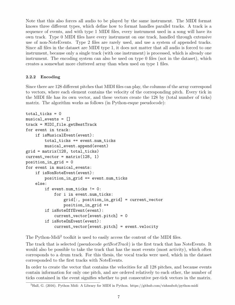
Since there are 128 different pitches that MIDI files can play, the columns of the array correspondto vectors, where each element contains the velocity of the corresponding pitch. Every tick inthe MIDI file has its own vector, and these vectors create the 128 by (total number of ticks)matrix. The algorithm works as follows (in Python-esque pseudocode):

total_ticks = 0

musical_events = []

track = MIDI_file.getBestTrack

for event in track:

if isMusicalEvent(event):

total_ticks += event.num_ticks

musical_event.append(event)

grid = matrix(128, total_ticks)

current_vector = matrix(128, 1)

position_in_grid = 0

for event in musical_events:

if isNonNoteEvent(event):

position_in_grid += event.num_ticks

else:

if event.num_ticks != 0:

for i in event.num_ticks:

grid[:, position_in_grid] = current_vector

position_in_grid ++

if isNoteOffEvent(event):

current_vector[event.pitch] = 0

if isNoteOnEvent(event):

current_vector[event.pitch] = event.velocity

The Python-Midi2 toolkit is used to easily access the content of the MIDI files.

The track that is selected (pseudocode getBestTrack) is the first track that has NoteEvents. Itwould also be possible to take the track that has the most events (most activity), which oftencorresponds to a drum track. For this thesis, the vocal tracks were used, which in the datasetcorresponded to the first tracks with NoteEvents.

In order to create the vector that contains the velocities for all 128 pitches, and because eventscontain information for only one pitch, and are ordered relatively to each other, the number ofticks contained in the event signifies whether to put consecutive per-tick vectors in the matrix.

2Hall, G. (2016). Python Midi: A Library for MIDI in Python. https://github.com/vishnubob/python-midi

7

Figure 1: A visualization of a MIDI file. The darkness of the blue cells indicates the velocity (volume)of the tone. Only twelve of 128 possible pitches are depicted. In this image, each bar is 1 tick.

Figure 2: An example of MIDI events converted to a 2 dimensional matrix. For demonstrativepurposes, only the first 5 pitches (instead of 128) are shown. The rest is all zeros.

Vectors are added when the number of ticks in an event does not equal zero, because this meansthat this event (relative to the previous event) is triggered later, so vectors are copied for thisduration. Once vector placement is handled, the vectors can be changed for the next event. Avelocity of 0 means that sound that was playing previously will no longer play. This is usuallyhandled by a NoteOffEvent, but it is also possible to do this by having a NoteOnEvent with0 velocity. The final line in the pseudo-code simply places the velocity of an event’s specifiedpitch in the to-be-placed vector, covering both cases. See Figures 1 and 2 for an example.

This algorithm encodes the MIDI file into a two dimensional array. This array can then be fedinto the LSTM network described in Section 2.3.2.

2.2.3 Decoding

The array can also be decoded back into a MIDI file. The algorithm for this process is usedafter predictions are made, and converts a matrix of predicted ticks into a MIDI file, so thatit can be played back. This prediction process is described in Section 2.5. The algorithm fordecoding the arrays is (once again in Python-esque pseudocode) shown below:

track = newMIDITrack()

previous_vector = grid[0] # first vector

for note_index in previous_vector:

if note_velocity != 0:

track.append(NoteOnEvent(0, previousvector[note_index], note_index))

tickoffset = 0

for vector in grid:

if previousvector == vector:

tickoffset ++

else:

for note_index in previous_vector:

if previousvector[note_index] == vector[note_index]:

8

continue

if previousvector[note_index] != 0 and vector[note_index] == 0:

track.append(NoteOffEvent(tickoffset, note_index))

else:

track.append(NoteOnEvent(0, vector[noteindex], note_index))

tickoffset = 0

tickoffset ++

previousvector = vector

The decoding algorithm starts by taking the content of the first vector in the array and triggeringall corresponding events (for all non-zero elements). Afterwards, using a tickoffset, all vectors areiterated and compared. When consecutive vectors are identical, the tickoffset simply increases.Otherwise, the content is compared. Any elements that are not equal will trigger another event.This is either a NoteOffEvent if a pitch in the previous vector was non-zero and in the currentvector is zero, or a NoteOnEvent otherwise. The tickoffset must be reset after any possiblechange within one vector, in order to maintain a relative relation between events.

2.3 LSTM Network

2.3.1 Background

A recurrent neural network (RNN) is a type of network that uses memory, as it learns to encodethe transitions in temporal, sequential data. This is done by having nodes combine informationfrom previous time steps with information in their current input. However, this type of networkstruggles with learning long-term dependency [11], meaning that relations learned relatively longago tend to have low weights, as the weights decrease over time. This problem is solved in LongShort-Term Memory (LSTM) networks.

Figure 3: A visualization of a module in an average LSTM. The cell state is the top horizontal line.It receives information from the second state, the line through the bottom. Both states received

input from the previous module, but the second state receives additional input (Xt) and providestemporary output (ht). The image is from a 2015 blog by C. Olah3.

3 Olah, C. (2015). Understanding LSTM Networks. http://colah.github.io/posts/2015-08-Understanding-LSTMs/

9

Like regular recurrent neural networks, LSTM networks are built from neural network chains.The difference is that in regular RNNs, the networks are built from a simple structure (such asa module containing one layer that performs a computation between nodes), while in LSTMsthe modules are built around a cell state, which is one of two managed states in the module(see Figure 3). The cell state contains the memory of the RNN. It is created by forwarding theoutput of the previous module, and receives information from the second state before forwardingitself to the cell state of the next module. The second state takes input (this is the input givento regular neural networks) and performs specific computations that determine what part of thenew input is fed into the cell state (the memory), and to determine what part is then returnedas momentary output. The exact computations may differ between LSTM implementations,but the standard framework is as follows:

• A calculation determines what information in the cell state should be forgotten, so thatnew information can take its place (this could for example be determined by calculatingvariance). This is the forget gate. In a standard LSTM network, this can be calculatedwith:

ft = σ(Wf · [ht, xt] + bf )

Where σ refers to a sigmoid function. f determines what is being forgotten. Since asigmoid is used, this value is between 0 and 1, and this range corresponds to how much isforgotten: the smaller the value, the more is forgotten (removed from the cell state). W isthe corresponding weight of the neural network node. x and h are inputs, x correspondingto new input and h being forwarded from the previous module. b is a constant.

Figure 4: This illustration depicts the forget gate.

• A combination of determining what information in the cell state will be updated, anddetermining what information (from the input) then overwrites it in the cell state. This isthe input gate. The result of these combinations are then added (mathematical addition)on to the new cell state. This addition solves the problem of vanishing gradients whichoccurs in different types of (recurrent) neural networks, as instead of possibly multiplyingvery small numbers (leading too smaller numbers, and thus the vanishing gradient), theyare added. In a standard LSTM network, the calculations are:

it = σ(Wi · [ht−1, xt] + bi)C̃t = tanh(WC · [ht−1, xt] + bC)

10

Figure 5: These illustrations depict the input gate.

This determines which part is updated. Here i is the information that is being input toreplace what was previously forgotten, C is the new cell state. tanh can be used to geta value between −1 and 1, if the network is built for such a range. With these values,updating the cell state follows:

Ct = ft ∗ Ct−1 + it ∗ C̃t

The f calculated previously is multiplied by the previous cell state, and then added to anew cell state i ∗ C̃.

• A combination of calculating what part from the second process is outputted and whatpart of the cell state. These calculations are multiplied, and the result is sent to theoutput, as well as to the second process of the next module. This is the output gate. In astandard LSTM network, this is calculated as:

ot = σ(Wo[ht−1, xt] + bo)ht = ot ∗ tanh(Ct)

Here o is the proposed output, which when multiplied by the cell state creates a statewhich can be sent to the output node of the network, and is also sent to the next module(where the entire process starts again).

Figure 6: This illustration depicts the output gate.

While the exact order of these gates may differ between LSTM implementations, the forgetgate generally comes before the input gate, as otherwise the network may forget what it just

11

learned. By having the output gate last, modules output what was learned during their owncycle.

What has been described above is the standard LSTM network, and the one that is used inthis thesis. It is implemented in Python using the Keras4 and Theano [13] frameworks.

2.3.2 Implementation

The network was made up of 3 layers, as shown in Figure 7. The input was entered into anLSTM layer with 512 nodes. Next, dropout regularization was used in order to reduce overfitting[14], after which there was another LSTM layer with 512 nodes. A Dense layer then lowered thenumber of nodes to 128 (corresponding to 128 possible pitches), which was sent to the output.This structure was determined through experimentation. Mean squared error was used as lossfunction for training, with linear activation. RMSProp optimization [12] was used to speed upthe training of the network.

Figure 7: A visualization of the layers of the neural network. The first LSTM layer with 512 nodes isgiven 2-dimensional arrays created from encoded MIDI files. Dropout regularization is performedafterwards, followed by another LSTM layer with 512 nodes. A dense layer then connects these

nodes into 128x1 vectors, for output.

The network trains on a collection of MIDI files. Each of these files is converted into a matrix asdescribed in the previous section. The content of these matrices is then copied into sequencesof input vectors each with a corresponding label vector. The length of these sequences shouldbe sufficiently large so that the input vectors encompass different pitches (ideally, a change inmelody), but not so large that it fails to find relation between input and label (leading to highloss in the loss function). The label vector is the vector that is one column further than thelast of the sequence vectors in the matrix.

Figure 8: A visualization of selecting the input and label vectors from a converted MIDI matrix. Inred, a sequence of vectors are selected for input (with sequence length 9). In blue, the label vector is

selected.

4 Chollet, F. (2016). Keras: Deep Learning library for Theano and TensorFlow. http://keras.io//

12

Although specific sequence sizes were determined through experimentation, it is worthwhile touse multitudes of 12, because (as was mentioned earlier) the ticks in MIDI format correspondthrough MIDI resolution to number of pulses per quarter note, and 12 can be divided by both4 and 6, which allow different musical tempos to be incorporated. However, the music in thedataset could be incorporated using multitudes of 4, which was why all sequences sizes usedwere multitudes of 4.

After selecting one sequence of input and label vectors, the selection moves a specified step sizeof columns to the right and then selects the next sequence of input vectors and the correspondinglabel vector. These sequences and vectors are added to two lists. Once all files in the datasethave been processed, batches of the sequences and label vectors are entered into the neuralnetwork. Doing this in batches is necessary because of hardware limitation, as processing toomany sequences at once will quickly overflow CPU RAM. The network trained 50 epochs on eachbatch. Training and predicting was done on the Distributed ASCI Supercomputer 4 (DAS-4)5.

2.4 Variants

Four different variations for handling the previously described batches were implemented, inorder to gauge how these would affect the quality of the generated music.

• Regular/standard batch selection: Batches were selected consecutively from the encodedmusic arrays. The size of each batch/sequence was 64 vectors. This means that all possiblesequences of 64 vectors (plus one label vector for each sequence) in a song are learned bythe neural network.

• Removing zero vectors: Music sometimes involves periods of silence, and this is particularlycommon in vocal tracks (including the vocal tracks from the dataset). In an encoded array,these periods are represented by consecutive zero vectors. While learning silent periods(and the transition to and from these) may be useful (especially with significantly largerdatasets), it may also lead to the network favoring the predicting of long periods of silencebecause of how similar the sequence and corresponding label vector will be. For thisreason, a variation on the handling of batches for training is to remove all zero vectorsfrom the encoded array.

• Larger sequence sizes: Different sizes for the sizes of the selected batches/sequences wereimplemented (mainly because of an issue with looping predictions that will be describedin Section 3). Sequence sizes of 96 (medium) and 160 (large) were used, in an attempt tolower overfitting and learn larger musical structures.

• Random batch selection: Instead of using a step size between consecutive batches ofvectors, this variation on handling batch selection selected 1000 random batches from anencoded array, for every musical file in the dataset, in another attempt to reduce possibleoverfitting, and perhaps bolster the creativity of the network. With a sequence size of 64,most files in the dataset contained between 3 and 5 thousand possible batches, meaningthat the network trained significantly less than when using regular batch selection. Thus,another variation took 3000 random batches instead of 1000.

2.5 Prediction

Once training is complete, the prediction process can begin. This is based on a small segmentof an input song, in the same per-tick array format that was used for the songs during training.

5 DAS-4: A six-cluster wide-area distributed system for researchers. http://www.cs.vu.nl/das4/

13

The same sequence length used then is used now to determine the size of the segment. Withthis as a matrix and the learned weights, a new vector is predicted, corresponding to the nexttick of music. The values of these vectors should be those that the network deemed most likelyto follow the segment (determined by the loss function during training).

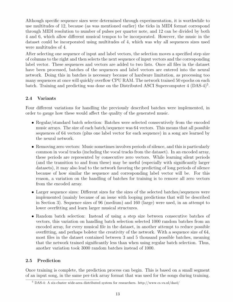
After a vector has been predicted, every vector in the array that corresponded to the inputsegment is pushed one position (column-wise) to the left, and its first vector is removed. Thepredicted vector then becomes the last vector (furthest to the right) in the array. With thisarray, another vector is then predicted, and the array is adjusted again. By repeating thisprocess, sequential music may be generated.

Figure 9: A visualization of predicting a vector that follows an array. The vectors are pushed to theleft and the predicted vector joins the array. Another new vector can then be predicted, leading to

another changed array. The sequence length here is 5.

Every predicted vector is stored in a separate list so that the entire prediction, as an array, canthen be converted into a MIDI file. The values inside the vectors may need to be clipped, tonot be lower than 0 or higher than 127, due to the nature of the linear-based neural network.

2.6 Post-processing

After predicting has finished, some post-processing may be necessary, in order to smooth pre-dicted vectors so that minor differences in pitches are replaced by consecutive same pitches,which sounds better. This is done by looking at every velocity for every vector in the arrayof predictions. For every possible pitch, the highest occurring velocity over the entire array isfound and stored.

Next, the velocity values of every pitch for every vector is compared to the highest occurringvelocity on that pitch. If the difference between the two velocities is higher than 10% of thehighest occurring velocity on that pitch, the velocity for that pitch in the corresponding vectoris set to 0. Otherwise, the velocity is set to 100. This causes all velocity values in the eventualfile to be 100, which is a velocity that is used commonly in MIDI files (most of the files in thedataset used in this thesis only contain velocity values of 100).

Using this percentage-based comparison is necessary to capture pitches that were deemed lesslikely during prediction but still somewhat important to the melody (e.g. a supporting melody

14

on the background). Using a constant comparison threshold would fail to capture these, orcause high velocity values to become single long pitches (due to small differences being seen asinsignificant and thus being smoothed).

In addition to this method of smoothing, very low velocity values are removed altogether. Thesevalues correspond to the network determining that a pitch is extremely unlikely. If left in thearray, it becomes soft background noise. By using the highest occurring velocity value for everypitch, it is easy to determine whether or not a pitch contains any relevant music. If the highestoccurring velocity is lower than 5, all velocity values on that pitch for every vector in the arrayare set to 0.

Figure 10: A visualization of a predicted song before and after post-processing.

It is worth noting that with more training and especially with a larger dataset, the amount ofpost-processing required may be greatly reduced.

3 Results

Evaluation is difficult for this thesis, as music is subjective. Nevertheless, the predicted musicmay be analyzed and apparent structure through common occurrences may be inferred, whichwill be handled first: The results of four variants of batch selection are examined, and this isfollowed by an analysis.

Afterwards, an empiric study in the form of a survey is processed, with the goal to objectivelyanalyze the subjective music.

3.1 Standard Batch Selection

With standard batch selection, structured music appeared to be generated with the example.midfile as input (see Figure 11). The generation starts out with a short period of disorganized noise,which also happens when using jono.mid and stella.mid as input (Figure 12). These two fileshowever fail to generate anything other than silence with extremely low velocity values whichare filtered out during post-processing. With stair.mid (Figure 13), the generation resemblesthe beginning of Stairway to Heaven for approximately 288 ticks, until it becomes disorganizednoise. While it eventually breaks out of this and begins a structured melody, this does notresemble the original song.

15

Note that in the following figures, the input music (in the first 64 ticks) may not completelyresemble the content of the input music as can be found in the Appendix. This is becauseduring post-processing, some parts of the input may have been filtered out. This does notmean that it was not completely used during generation, however, as post-processing occursafter the prediction process has finished.

Figure 11: A visualization of the predicted music using regular batch selection with example.mid asinput. The segments separated by grey vertical lines contain 32 ticks. The input music is shown inthe first 64 ticks. The generated music (which begins on tick 64) starts out noisy and disorganized,

before settling into a melody on tick 135.

Figure 12: Visualization using regular batch selection with jono.mid (left) and stella.mid (right) asinput. Both contain only a short sequence of disorganized noise, and failed to generate further.

16

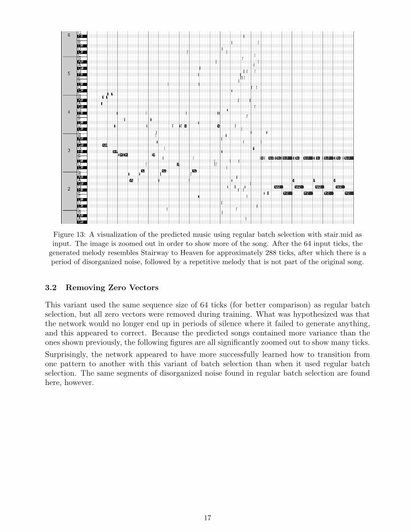
Figure 13: A visualization of the predicted music using regular batch selection with stair.mid asinput. The image is zoomed out in order to show more of the song. After the 64 input ticks, the

generated melody resembles Stairway to Heaven for approximately 288 ticks, after which there is aperiod of disorganized noise, followed by a repetitive melody that is not part of the original song.

3.2 Removing Zero Vectors

This variant used the same sequence size of 64 ticks (for better comparison) as regular batchselection, but all zero vectors were removed during training. What was hypothesized was thatthe network would no longer end up in periods of silence where it failed to generate anything,and this appeared to correct. Because the predicted songs contained more variance than theones shown previously, the following figures are all significantly zoomed out to show many ticks.

Surprisingly, the network appeared to have more successfully learned how to transition fromone pattern to another with this variant of batch selection than when it used regular batchselection. The same segments of disorganized noise found in regular batch selection are foundhere, however.

17

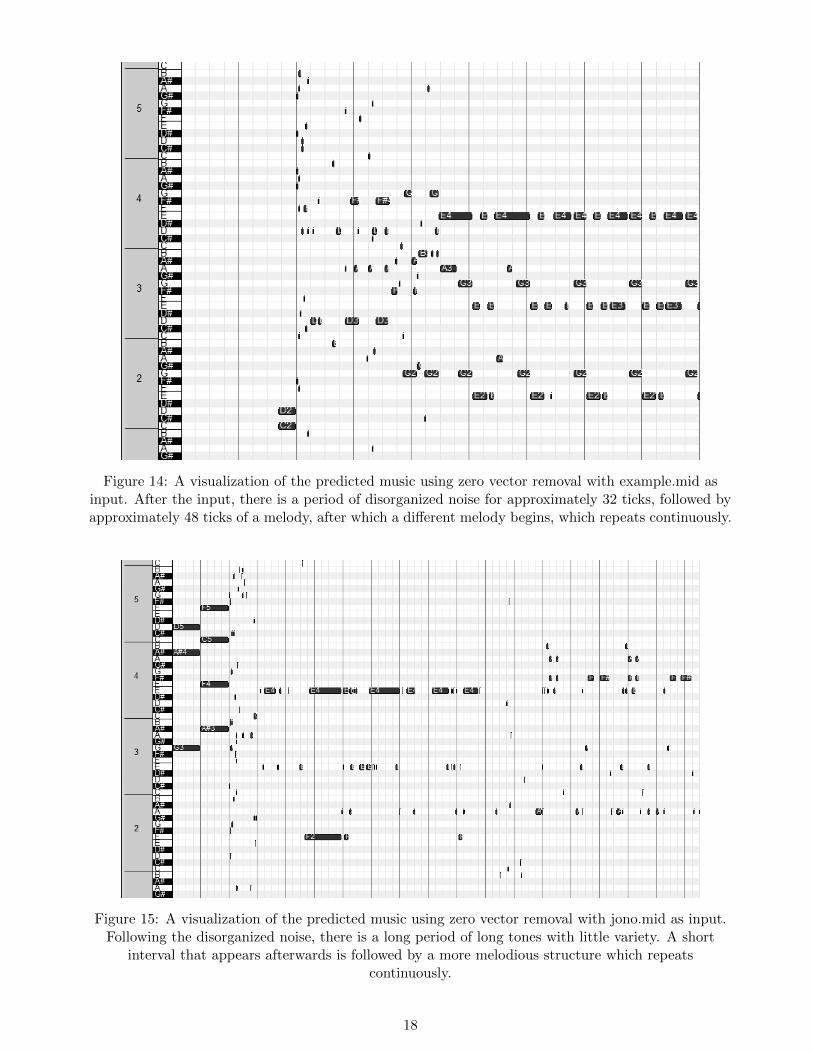
Figure 14: A visualization of the predicted music using zero vector removal with example.mid asinput. After the input, there is a period of disorganized noise for approximately 32 ticks, followed byapproximately 48 ticks of a melody, after which a different melody begins, which repeats continuously.

Figure 15: A visualization of the predicted music using zero vector removal with jono.mid as input.Following the disorganized noise, there is a long period of long tones with little variety. A short

interval that appears afterwards is followed by a more melodious structure which repeatscontinuously.

18

Figure 16: A visualization of the predicted music using zero vector removal with stella.mid as input.While a lot is generated (once again after a very short period of disorganized noise), it is very

repetitive and filled with outliers.

Figure 17: A visualization of the predicted music using zero vector removal with stair.mid as input.The prediction resembles Stairway to Heaven only in the very beginning for 96 ticks. A simplepattern follows, there is a very melodious segment for 160 ticks before transitioning back to the

simple pattern. This melody is not part of the original song, however.

19

3.3 Larger Sequence Sizes

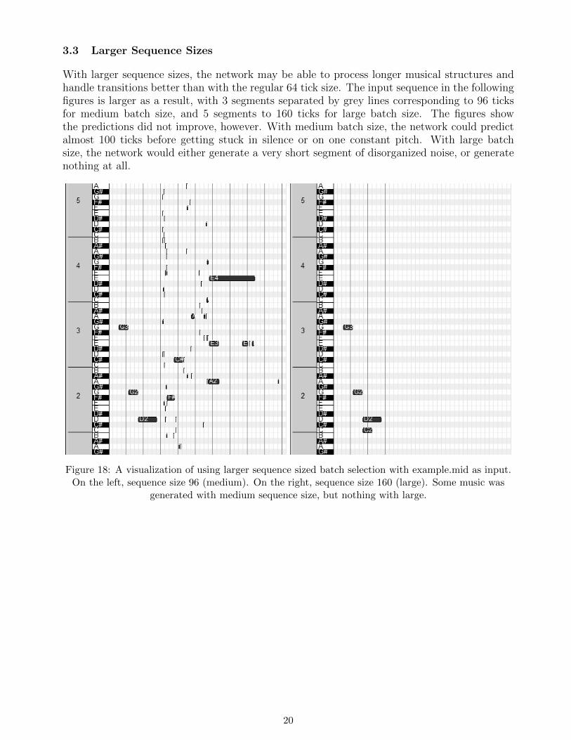
With larger sequence sizes, the network may be able to process longer musical structures andhandle transitions better than with the regular 64 tick size. The input sequence in the followingfigures is larger as a result, with 3 segments separated by grey lines corresponding to 96 ticksfor medium batch size, and 5 segments to 160 ticks for large batch size. The figures showthe predictions did not improve, however. With medium batch size, the network could predictalmost 100 ticks before getting stuck in silence or on one constant pitch. With large batchsize, the network would either generate a very short segment of disorganized noise, or generatenothing at all.

Figure 18: A visualization of using larger sequence sized batch selection with example.mid as input.On the left, sequence size 96 (medium). On the right, sequence size 160 (large). Some music was

generated with medium sequence size, but nothing with large.

20

Figure 19: A visualization of using larger sequence sized batch selection with jono.mid as input. Onthe left, sequence size 96 (medium). On the right, sequence size 160 (large). Medium sequence sizegenerated some structure (with pitches being turned sporadically on and off). Large sequence size

generated mostly noise, before stopping generation altogether.

Figure 20: A visualization of using larger sequence sized batch selection with stella.mid as input. Onthe left, sequence size 96 (medium). On the right, sequence size 160 (large). Again, little is

generated, with medium sequence size getting stuck on one constant pitch, and large generating afew sporadic tones.

21

Figure 21: A visualization of using larger sequence sized batch selection with stair.mid as input. Onthe left, sequence size 96 (medium). On the right, sequence size 160 (large). With medium sequence

size, the prediction slightly resembles the original song only in the very beginning. With largesequence size, only noise is generated.

3.4 Random Batch Selection

This variant of batch selection was attempted with 1000 randomly selected batches as well as3000. Because the network failed to predict anything with many input songs for both of theseattempts, only three of the results are shown in the following figures. Large batch size was usedfor all these, which means the input size is 160 ticks and corresponds to 5 segments separatedby grey vertical lines.

Figure 22: A visualization of the predicted music using 1000 randomly selected batches withjono.mid as input. The prediction gets stuck on the same pitches and predicts these continuously.

22

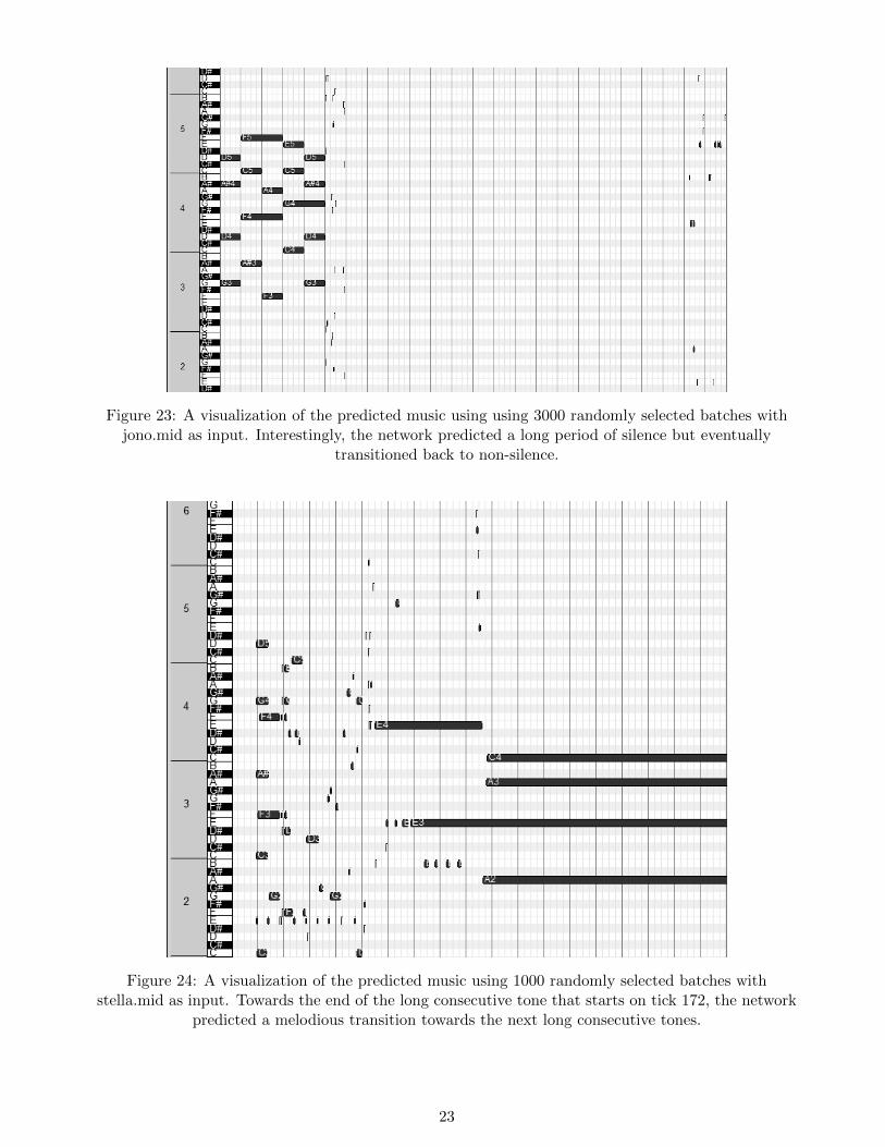
Figure 23: A visualization of the predicted music using using 3000 randomly selected batches withjono.mid as input. Interestingly, the network predicted a long period of silence but eventually

transitioned back to non-silence.

Figure 24: A visualization of the predicted music using 1000 randomly selected batches withstella.mid as input. Towards the end of the long consecutive tone that starts on tick 172, the network

predicted a melodious transition towards the next long consecutive tones.

23

3.5 Evaluation

With regular batch selection, both the generation that used jono.mid and the generation thatused stella.mid were unable to generate much beyond the small segments of disorganized noise.This may have been because of the vocal tracks that were used for training. Vocal tracks containlong periods of silence, which may have led to the network ending up stuck in a sequence ofcontinuing predicted silence, as its memory is not large enough to enclose transition into non-silence again. The batch selection variant where zero vectors are removed was created as apossible way to address this.

A possible explanation for the generation of disorganized noise (found in all of the variants ofbatch selection) is that the LSTM network failed to find a connection between its short memoryof input ticks and what it had learned during training from the dataset, as the input music iseither in a key that no music in the dataset is ever in, or is not in a key at all (in the caseof example.mid, which is just a few random tones). Since the network does not recognize thekey, it fails to find one likely pitch, and instead returns many unlikely ones. This is continueduntil a pattern emerges which the network can recognize, and a learned structure follows. Thisexplanation is backed up by the fact that with regular batch selection, the network did not havetrouble continuing Stairway to Heaven (until as the generation continued, it became harder andharder to further the original song), as it recognizes the key in the input music, which is in thedataset.

With regular batch selection, the generations eventually end up with a repeating structure aftera period of disorganized noise. While this may imply that the network correctly learned musicalstructure, an infinite repetition of a very short melody is monotonous, and not somethingfound in songs in the dataset. Ideally, the network should transition into different melodiousstructures. The reason this happens may be that certain structures that were learned duringtraining fit exactly into the specified sequence size (batch): If a melodious structure occursconsecutively in a dataset, and one occurrence fits exactly within the sequence size, then atthe end of having predicted the structure, the network may find it likely that this is the firstoccurrence, and that it should repeat it. Since the sequence size determines the memory of thenetwork, it is incapable of remembering that it has already predicted the structure multipletimes. Larger sequence sizes however failed to generate much music due to large segments ofdisorganized noise, so it is difficult to say with these results whether larger sequence sizes willhelp reduce repetition and inspire transition.

In general, with larger sequence sizes, specifically with a size of 160 ticks, the network hada much more difficult time generating music (it did not generate anything at all with theexample.mid file). This may mean that finding the correct musical key gets more importantthe larger the sequence size is. It may also be possible that because the example file is not longenough to make up the entire 160 tick input segment and zero vectors had to be appended,that the network had too many zero vectors in its input, and generated only silence because ofthis. This does not explain the issues with the other files, however.

With random batch selection, the number of periods of disorganized noise was much smallerthan with other variants of batch selection. However, in the few cases that the network didmanage to predict music, the prediction would often get stuck on the same pitches. This may bebecause transitions are more difficult to learn when randomly selecting batches. While, one ofthe generated songs did contain a melodious transition of one structure to another, this may justbe the result of having randomly found some structure with this transition that also occurredin other randomly selected batches during training. It is difficult to interpret the results of therandom selection when it failed to predict music so often.

Many of the predicted songs (with all variants of batch selection) contained outliers. While

24

it may be possible to filter some of these out using different threshold values during post-processing, it should be noted that the pitches of these outliers were always still close to thepitches of whatever main pattern the predicted songs created. No pitch was ever further than20 pitches away from the highest pitch found in its main pattern. This may not imply that thenetwork had started learning how to work within musical key, but it did learn that extremepitches are very unlikely in music, or at least in the type of music that fits the dataset.

From these results, removing zero vectors appears to have led to the best predictions. Musicalstructure appear melodious and there are transitions between patterns. However, music remainssubjective, and while the generated music from zero vector removal may look structurallycorrect, it is still up to people to decide the subjective quality of the songs.

3.6 Survey

Ten participants were asked to listen to samples of 9 generated songs:

1. Regular batch selection with example.mid

2. Regular batch selection with stair.mid

3. Zero vector removal with example.mid

4. Zero vector removal with jono.mid

5. Zero vector removal with stella.mid

6. Zero vector removal with stair.mid

7. Medium sized batch selection with jono.mid

8. Medium sized batch selection with stair.mid

9. Random batch selection with stella.mid

For each sample, participants were asked to grade the pleasantness of the sample on a grade of1 to 5, with 5 being most pleasant. The average grade of each sample was:

example.mid jono.mid stella.mid stair.mid

Regular 2.9 3.3Zero Vector Removal 3.3 3.6 2.3 2.0Medium Batch Size 2.3 2.4Random Batch Selection 3.2

Zero vector removal received the highest individual average grade, while medium sized batchselection received the lowest grades averaged over its two samples. This is consistent with theexamination of the structure of the predictions, where predictions using zero vector removalappeared the most melodious. The network failed to generate much music with larger batchsize selection, and what it did generate was often very noisy, so this is also consistent.

25

4 Discussion

While the created format for representing MIDI files can be successfully implemented in theLSTM network, it can only handle one channel (MIDI channels usually represent differentinstruments). In order to handle multiple channels, the algorithm would either need to berewritten to construct a higher dimensional grid (one dimension is added, with the differentchannels as its axis), or the values in the 2-dimensional grid that is used now (the velocity(loudness) of the notes) need to have a system where ranges of values map to different channels.A possible method for doing this would involve having each channel receive its 128 notes, wherehigher channels start with a value 128 higher than the previous channel. Then the channel thatthe value maps to can be found by dividing by 128, and the value by using the modulo operatorwith 128.

The MIDI encoding system cannot handle consecutive same-velocity and same-pitch tones.While such tones are rare (it is impossible for acoustic music, as no human can stop and startplaying an instrument at the same time), it does occur in some electronic music. These tones,after being encoded, become one continuous tone. This is a limitation of the algorithm. Apossible solution would involve pre-processing where MIDI files are checked for this behavior,and manually setting the sequence of velocity values one higher or lower than the previoussequence.

The Keras framework was used because it enables high level implementations of difficult con-cepts. This meant that more time could be spent on other parts of the thesis. However, theframework is stuck with a somewhat fixed system of relation between input and output (e.g. thesequence length must remain constant throughout). This could be circumvented by changingsource code manually, which defeats the purpose of saving time because it would take a lot oftime to understand. This fixed system meant that various experiments, such as experimentingwith alternating sequence lengths, or having output that were longer than one vector (arraysas output), were not possible. Some RNN implementations rely on output sequences, whichare not possible in Keras, but may be beneficial for the topic of this thesis and future work.Thus, future research should experiment with different frameworks that allow more sequentialoutput.

Though different variants of batch selection were explored, they all ignored the use of a variablestep size between batches. Random batch selection does not use a step size at all, and the othervariants all used a step size of 1. Early on during experimentation a step size of 1 appeared tomore successful than larger step sizes, which led to future experimenting with other step sizesbecoming an afterthought. Nevertheless, it may be worthwhile to do more experimentationwith larger step sizes on different datasets. In particular, this may be effective for songs withhighly repetitive structure, as batches may skip over some of these parts. It may also helpin lowering the likelihood of music generation getting stuck in loops, albeit at the risk of lesslearned structure. Also of note is that larger step sizes will reduce the total number of trainedbatches, which may greatly reduce the time the network has to spend training.

Post-processing proved useful in filtering out noise and in smoothing velocity values. However,in many predictions, some very short tones (usually of only one tick) still occurred sporadicallythroughout the entire predicted song. These tones were almost always off-key. While exper-imenting further with the current method of post-processing (increasing the minimum valuethreshold, and increasing the percentage of allowed difference between the highest and the pro-cessed velocity values) may result in better results, adding a new step to post-processing mayalso be beneficial. This new step would involve filtering out off-key velocity values. This wouldinclude determining the most recent key, and calculating whether predicted non-zero velocityvalues for pitches that had zero velocity values during the sequence are off-key compared to

26

the recent key. If they are, there can be another check to see if the vector could belong toa new sequence where the value would be in-key. If it fails both checks, the velocity can beset to 0. This will require a non-trivial function that determines whether a pitch is off-key orin-key given a sequence. However, there is some research into techniques for key detection [15].For the second check, defining whether a vector belongs to a new sequence may simply involvechecking further in the predicted array, as all this will be done in post-processing, which meansthat any vectors further into the array are already available.

Instead of doing the aforementioned during post-processing, it may also be interesting to makekey detection a primary focus for a future automated music generation study. If a neuralnetwork can use the sequence of musical keys detected in a dataset of songs for training, it maybe able to then randomly generate music in-key and then use the learned sequence transitionsto transition various keys into melodies and songs. While this does make the research moresimilar to other studies that have worked with grammars that already encapsulate a sequencebetween which pitches must remain (essentially a key), doing this with MIDI files may still beinnovative.

While the results of increasing sequence length and of using random batch selection to collecttraining sequences with corresponding label vectors were less than satisfactory, it is possiblethat increasing the size of the training set may significantly improve the results. With only 74files in the dataset, it becomes more difficult to find structure in longer sequences. In fact, alarger dataset may improve the results of all methods of training. The dataset may simply betoo small for the network to learn any generalizable structure. As explained in Section 2.1, thesmall dataset was chosen because of an expected similarity between songs when using only oneband or artists. Nevertheless, experimenting with much larger datasets may be worthwhile.

Another variant for batch selection that was briefly tested during experimentation was the use ofbinary velocity values. All non-zero velocity values in an encoded array would be set to 1. Thereasoning behind this at the time was that it may lower loss during training. This was scrappedwhen no immediate more successful predictions were made with this method than without it.However, it may still be interesting to look into this, as it may allow for a classification taskinstead of regression, where every pitch is a class. This would then allow more experimentationwith different loss functions and activations in the neural network as well.

Also, the variations on batch selection may be combined. While combinations such as selectingrandom batches after removing zero vectors from an encoded array were not attempted for thisthesis, they may provide interesting results. More experimentation with this may serve as abasis for future research.

For empirical evaluation with the survey, only a limited number of participants reviewed theselection of samples of predicted songs. Given the subjective nature of music and the problemswith justifying generalizing results of small samples to larger populations, it may be worthwhileto repeat the survey or create new surveys with a larger number of participants.

5 Conclusion

It was hypothesized that with a dataset of songs encoded in MIDI format that are properlyconverted to a system that a recurrent neural network can use for training, it should be possibleto generate polyphonic music from any MIDI file. Furthermore, the ways of handling theconverted dataset may affect the quality of the generated music.

A dataset of 74 Led Zeppelin songs in MIDI format was encoded into arrays and used by anLSTM network with three layers for training. After training, the network could predict how

27

an input song should continue. There were four different methods of selecting data from thearrays, which affected how well the network could generate music. The most successful of thesewas where periods of silence in the songs in the dataset were removed. The structure of thegenerated songs with this method appeared the most melodious. This was consistent with asurvey taken where the subjective quality of samples of generated music was better with thismethod than with the other methods. However, the generated music contains noise in theform of pitch outliers and the network struggles with repetitiveness, and this is reflected in themediocre grades the generated music received in the survey. While it is definitely possible togenerate music using LSTM networks trained per-tick on a MIDI collection with short musicsegments as input, as was the topic of this thesis, the algorithms should be improved uponbefore declaring that all musicians will soon be out of jobs.

References

[1] Zaripov, R. X. (1960). Об алгоритмическом описании процесса сочинения музыки (Onthe algorithmic description of the process of composing music). In Доклады АН СССР (Vol.132).

[2] Lonsdale, A. J., & North, A. C. (2011). Why do we listen to music? A uses and gratificationsanalysis. British Journal of Psychology, 102(1), 108-134.

[3] McCormack, J. (1996). Grammar based music composition. Complex systems, 96, 321-336.

[4] Fox, R., & Crawford, R. (2016). A Hybrid Approach to Automated Music Composition. InArtificial Intelligence Perspectives in Intelligent Systems (pp. 213-223). Springer InternationalPublishing.

[5] Schmidhuber, J. (2015). Deep learning in neural networks: An overview. Neural Networks,61, 85-117.

[6] Chen, C. C. J., & Miikkulainen, R. (2001). Creating melodies with evolving recurrent neuralnetworks. In Neural Networks, 2001. Proceedings. IJCNN’01. International Joint Conferenceon (Vol. 3, pp. 2241-2246). IEEE.

[7] Eck, D., & Schmidhuber, J. (2002). A first look at music composition using lstm recurrentneural networks. Istituto Dalle Molle Di Studi Sull Intelligenza Artificiale, 103. Chicago

[8] Franklin, J. A. (2006). Recurrent neural networks for music computation. INFORMS Journalon Computing, 18(3), 321-338.

[9] Sak, H., Senior, A. W., & Beaufays, F. (2014, September). Long short-term memoryrecurrent neural network architectures for large scale acoustic modeling. In INTERSPEECH(pp. 338-342).

[10] Johnston, L. (2016). Using LSTM Recurrent Neural Networks for Music Generation.

[11] Hochreiter, S., Bengio, Y., Frasconi, P., & Schmidhuber, J. (2001). Gradient flow inrecurrent nets: the difficulty of learning long-term dependencies.

[12] Dauphin, Y. N., de Vries, H., Chung, J., & Bengio, Y. (2015). RMSProp and equilibratedadaptive learning rates for non-convex optimization. arXiv preprint arXiv:1502.04390.

28

[13] Team, T. T. D., Al-Rfou, R., Alain, G., Almahairi, A., Angermueller, C., Bahdanau, D., ...& Belopolsky, A. (2016). Theano: A Python framework for fast computation of mathematicalexpressions. arXiv preprint arXiv:1605.02688. http://deeplearning.net/software/theano/

[14] Srivastava, N., Hinton, G., Krizhevsky, A., Sutskever, I., & Salakhutdinov, R. (2014).Dropout: A simple way to prevent neural networks from overfitting. The Journal of MachineLearning Research, 15(1), 1929-1958.

[15] Zhu, Y., Kankanhalli, M. S., & Gao, S. (2005, January). Music key detection for musicalaudio. In 11th International Multimedia Modelling Conference (pp. 30-37). IEEE.

Appendix

Input Files

Now follows a visualization for each of the four input files used for prediction.

Example File (example.mid)

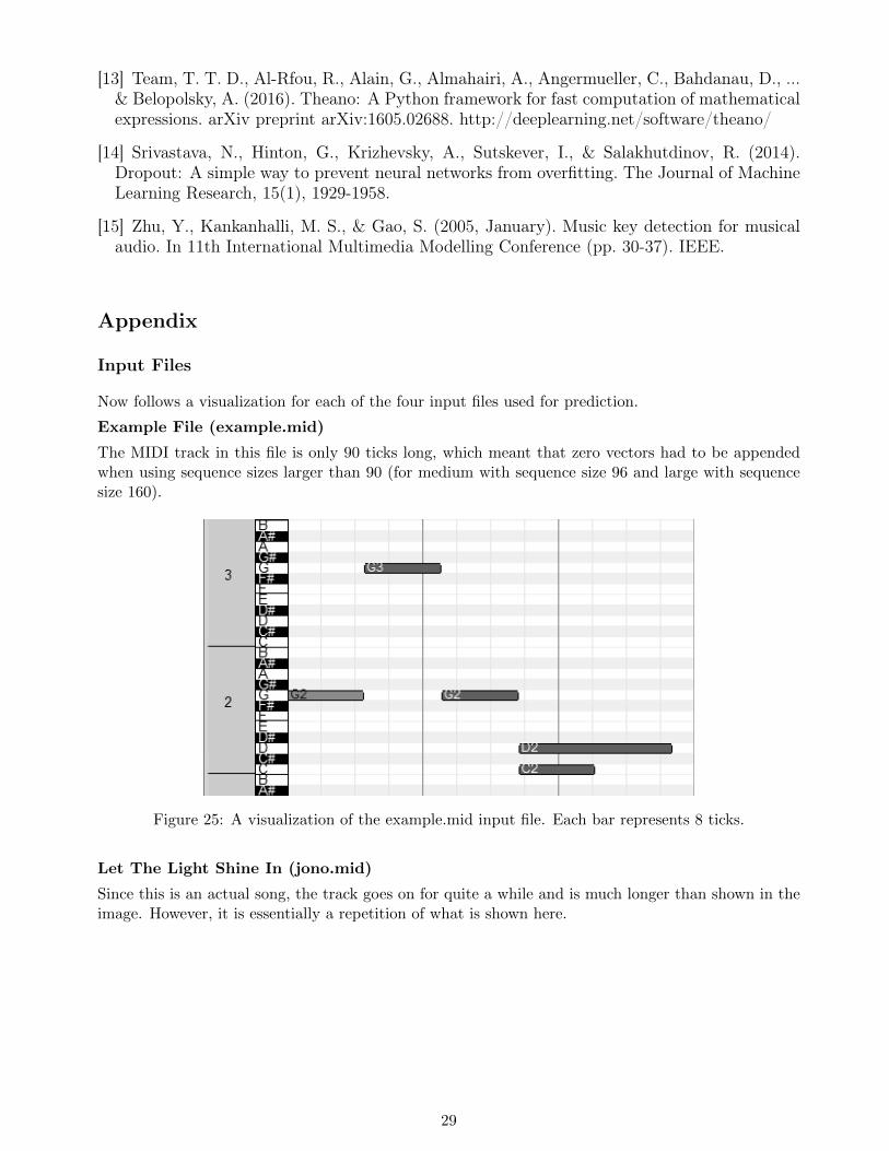
The MIDI track in this file is only 90 ticks long, which meant that zero vectors had to be appendedwhen using sequence sizes larger than 90 (for medium with sequence size 96 and large with sequencesize 160).

Figure 25: A visualization of the example.mid input file. Each bar represents 8 ticks.

Let The Light Shine In (jono.mid)

Since this is an actual song, the track goes on for quite a while and is much longer than shown in theimage. However, it is essentially a repetition of what is shown here.

29

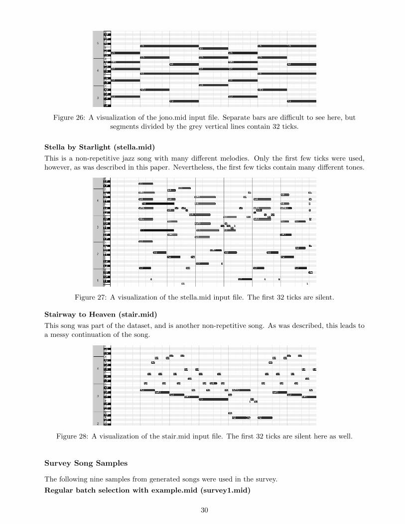
Figure 26: A visualization of the jono.mid input file. Separate bars are difficult to see here, butsegments divided by the grey vertical lines contain 32 ticks.

Stella by Starlight (stella.mid)

This is a non-repetitive jazz song with many different melodies. Only the first few ticks were used,however, as was described in this paper. Nevertheless, the first few ticks contain many different tones.

Figure 27: A visualization of the stella.mid input file. The first 32 ticks are silent.

Stairway to Heaven (stair.mid)

This song was part of the dataset, and is another non-repetitive song. As was described, this leads toa messy continuation of the song.

Figure 28: A visualization of the stair.mid input file. The first 32 ticks are silent here as well.

Survey Song Samples

The following nine samples from generated songs were used in the survey.

Regular batch selection with example.mid (survey1.mid)

30

Zero vector removal with example.mid (survey2.mid)

Zero vector removal with jono.mid (survey3.mid)

Medium sequence size batch selection with jono.mid (survey4.mid)

31

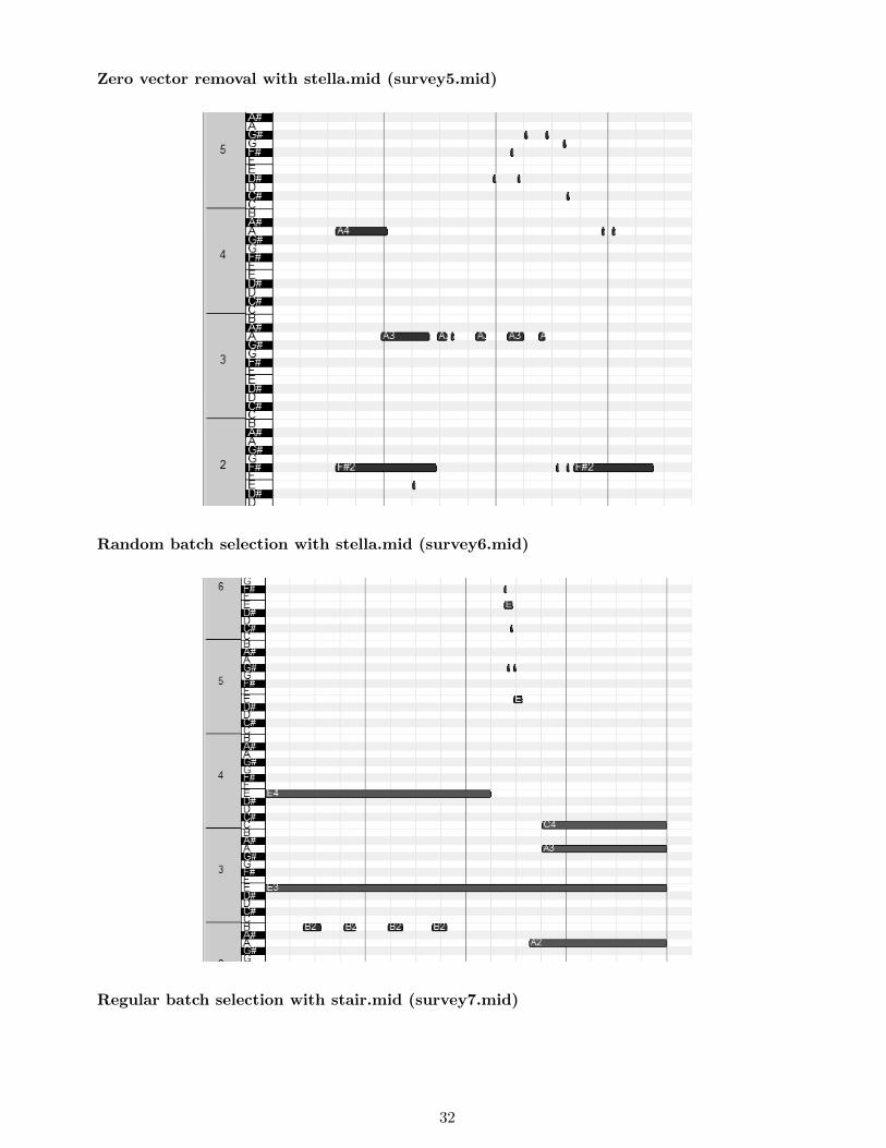
Zero vector removal with stella.mid (survey5.mid)

Random batch selection with stella.mid (survey6.mid)

Regular batch selection with stair.mid (survey7.mid)

32

Zero vector removal with stair.mid (survey8.mid)

Medium sequence size batch selection with stair.mid (survey9.mid)

33