Robot Manipulators Position, Orientation and Coordinate Transformations Fig. 1: Programmable Universal Manipulator Arm (PUMA) A robot manipulator is an electronically controlled mechanism, consisting of multiple segments, that performs tasks by interacting with its environment. They are also commonly referred to as robotic arms. Robot manipulators are extensively used in the industrial manufacturing sector and also have many other specialized applications (for example, the Canadarm was used on space shuttles to manipulate payloads). The study of robot manipulators involves dealing with the positions and orientations of the several segments that make up the manipulators. This module introduces the basic concepts that are required to describe these positions and orientations of rigid bodies in space and perform coordinate transformations.
Transcript
Robot Manipulators Position, Orientation and Coordinate Transformations
Fig. 1: Programmable Universal Manipulator Arm (PUMA)
A robot manipulator is an electronically controlled mechanism, consisting of multiple segments,
that performs tasks by interacting with its environment. They are also commonly referred to as
robotic arms. Robot manipulators are extensively used in the industrial manufacturing sector
and also have many other specialized applications (for example, the Canadarm was used on
space shuttles to manipulate payloads). The study of robot manipulators involves dealing with
the positions and orientations of the several segments that make up the manipulators. This
module introduces the basic concepts that are required to describe these positions and
orientations of rigid bodies in space and perform coordinate transformations.
Manipulators
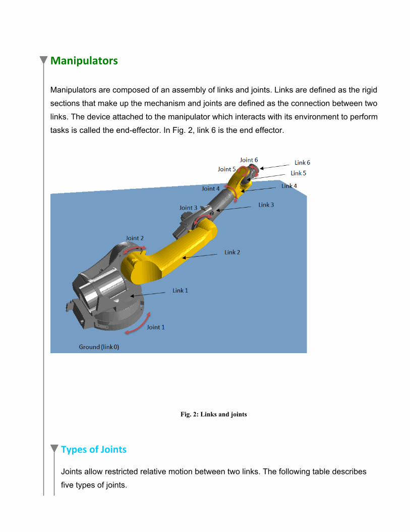
Manipulators are composed of an assembly of links and joints. Links are defined as the rigid
sections that make up the mechanism and joints are defined as the connection between two
links. The device attached to the manipulator which interacts with its environment to perform
tasks is called the end-effector. In Fig. 2, link 6 is the end effector.
Fig. 2: Links and joints
Types of Joints
Joints allow restricted relative motion between two links. The following table describes
five types of joints.
Table 1: Types of joints
Name of joint Representation
Description
Revolute Allows relative rotation about one axis.
Cylindrical Allows relative rotation and translation about one axis.
Prismatic Allows relative translation about one axis.
Spherical Allows three degrees of rotational freedom about the center of the joint. Also known as a ball-and-socket joint.
Planar Allows relative translation on a plane and relative rotation about an axis perpendicular to the plane.
Some Classification of Manipulators
Manipulators can be classified according to a variety of criteria. The following are two of
these criteria:
By Motion Characteristics
Planar manipulator: A manipulator is called a planar manipulator if all the moving
links move in planes parallel to one another.
Spherical manipulator: A manipulator is called a spherical manipulator if all the links
perform spherical motions about a common stationary point.
Spatial manipulator: A manipulator is called a spatial manipulator if at least one of
the links of the mechanism possesses a general spatial motion.
By Kinematic Structure
Open-loop manipulator (or serial robot): A manipulator is called an open-loop
manipulator if its links form an open-loop chain.
Parallel manipulator: A manipulator is called a parallel manipulator if it is made up of
a closed-loop chain.
Hybrid manipulator: A manipulator is called a hybrid manipulator if it consists of
open loop and closed loop chains.
Degrees of Freedom
The number of degrees of freedom of a mechanism are defined as the number of
independent variables that are required to completely identify its configuration in space.
The number of degrees of freedom for a manipulator can be calculated as
... Eq. (1)
where is the number of links (this includes the ground link), is the number of joints,
is the number of degrees of freedom of the joint and is for planar mechanisms and for spatial mechanisms.
Vector Kinematics and Coordinate Transformations
This section covers the concepts required to specify the location of an object in space. This
involves specifying the position of a point on the object and the orientation of the object with
respect to a reference frame.
Description of a Position
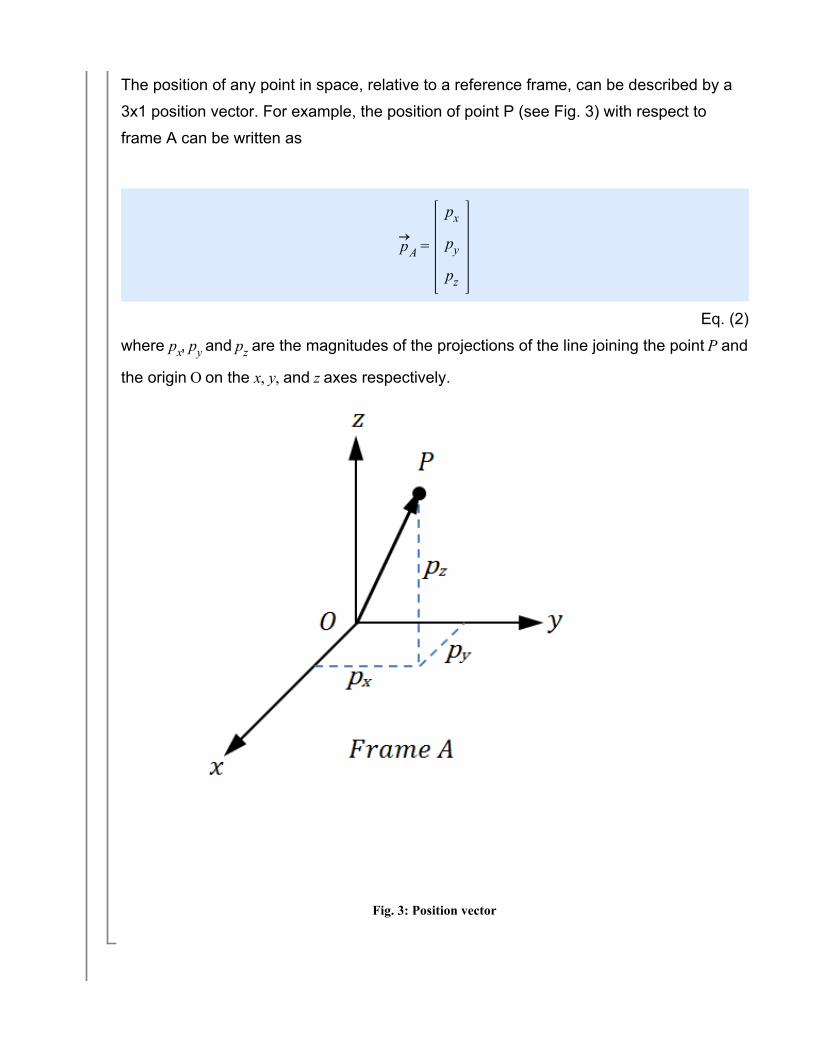
The position of any point in space, relative to a reference frame, can be described by a
3x1 position vector. For example, the position of point P (see Fig. 3) with respect to
frame A can be written as
Eq. (2)
where , and are the magnitudes of the projections of the line joining the point and
the origin on the and axes respectively.
Fig. 3: Position vector
Description of an Orientation
The orientation of a body in space can be described by attaching a coordinate system to
it and then describing the vectors of its coordinate axes relative to a known frame of
reference. For example, the coordinate axes of Frame B (see Fig. 4) can be described
relative to a known coordinate system A by the following unit vectors:
... Eq. (3)
These three vectors can be combined to achieve a 3x3 matrix called a rotation matrix.
... Eq. (4)
3. 3.
1. 1.
2. 2.
Fig. 4: Components of the rotation matrix of Frame B w.r.t Frame A
Rotation Matrix Properties
All the columns of a rotation matrix are orthogonal to each other.
The determinant of a rotation matrix is 1.
The inverse of a rotation matrix is equal to its transpose.
... Eq. (5)
This means that the rotation matrix of Frame B with respect to Frame A is equal to the
inverse and the transpose of the rotation matrix of Frame A with respect to Frame B.
Principal Rotation Matrices
Rotation about the z-axis
If a reference frame (Frame A) is rotated by an angle about the z-axis to obtain a
new frame (Frame B), the rotation matrix of the new frame is
... Eq. (6)
Fig. 5: Rotation about the z-axis
Rotation about the y-axis
If a reference frame (Frame A) is rotated by an angle about the y-axis to obtain a
new frame (Frame B), the rotation matrix of the new frame is
... Eq. (7)
Fig. 6: Rotation about the y-axis
Rotation about the x-axis
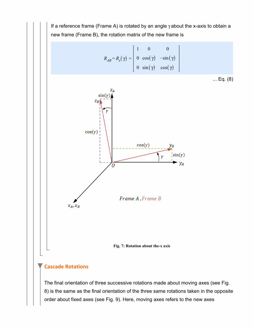
If a reference frame (Frame A) is rotated by an angle about the x-axis to obtain a
new frame (Frame B), the rotation matrix of the new frame is
... Eq. (8)
Fig. 7: Rotation about the-x axis
Cascade Rotations
The final orientation of three successive rotations made about moving axes (see Fig.
8) is the same as the final orientation of the three same rotations taken in the opposite
order about fixed axes (see Fig. 9). Here, moving axes refers to the new axes
obtained after each rotation.
Fig. 8: Three rotations about moving axes
Fig. 9: Three rotations about fixed axes
Mathematically,
... Eq. (9)
The following video shows a comparison of the final orientations of a coordinate
system after three successive rotations made about fixed and moving axes in the
same order. The frame on the right is rotated about its moving axes and the frame on
the left is rotated about fixed axes. The red axis corresponds to the x-axis, the green
axis corresponds to the y-axis and the blue axis corresponds to the z-axis (order of
rotations: 0.5 rad about z-axis, 0.75 rad about y-axis, 1 rad about x-axis).
Video Player
Video 1: Rotations about fixed and moving axes (some order).
As discussed above, since one frame rotates about its moving axes and the other
rotates about fixed axes, the two final orientations are different.
The next video also shows a comparison of the final orientations of a coordinate
system after three successive rotations made about fixed and moving axes. However,
for this case, the order of rotations for the frame rotating about fixed axes is the
opposite to the order for the frame rotating about its moving axes. The frame on the
right is rotated about its moving axes and the frame on the left is rotated about fixed
axes. Once again, the red axis corresponds to the x-axis, the green axis corresponds
to the y-axis and the blue axis corresponds to the z-axis (order of rotations for the
frame rotating about moving axes: 0.5 rad about z-axis, 0.75 rad about y-axis, 1 rad
about x-axis).
Video Player
Video 1: Rotations about fixed and moving axes (some order).
For this case, the orientations of both frames are the same at the end.
Steps to create the simulations
Euler Angle Representations
The Euler angle representations are commonly used representations that describe
orientations. These representations describe an orientation using three successive
rotations. Since rotation is a motion with three degrees of freedom, a set of three
independent parameters are sufficient to describe an orientation in space.
Roll-Pitch-Yaw Angles
This representation describes an orientation using a set of three successive
rotations about a fixed frame.
Fig. 14: Three rotations about fixed axes
The angle (rotation about the x-axis) is called the roll angle, the angle (rotation
about the y-axis) is called the pitch angle and the angle (rotation about the z
axis) is called the yaw angle.
The resulting rotation matrix of the three rotations is
... Eq. (10)
Since the multiplication of matrices do not usually commute, the order of the
rotations is important.
If a rotation matrix is given, the roll-pitch-yaw angles can be calculated using the
following equations:
... Eqs. (11) to (13)
where corresponds to the term in the row and column of the rotation
matrix.
z-y-z Euler Angles
This representation describes an orientation using a set of three successive rotations about moving axes.
Fig. 15: Three rotations about moving axes (z-y-z angles)
The resulting rotation matrix of the three rotations is
... Eq. (14)
If a rotation matrix is given, the z-y-z angles can be calculated using the following
equations:
... Eqs. (15) to (17)
Example 1: Euler Angles
(2.2.4.3.4)(2.2.4.3.4)
(2.2.4.3.1)(2.2.4.3.1)
(2.2.4.3.3)(2.2.4.3.3)
(2.2.4.3.2)(2.2.4.3.2)
(2.2.4.3.5)(2.2.4.3.5)
Problem Statement: The rotation matrix of Frame B with respect to a reference
frame A is . Find the roll-pitch-yaw angles and the z-y-z
angles.
Solution:The rotation matrix is:
The roll, pitch and yaw angles are (in rad):
1.099543058
1.410139396
0.7853981634
The z-y-z angles are (in rad):
1.244011150
0.5663241952
(2.2.4.3.6)(2.2.4.3.6)0.3457940165
Coordinate Transformations
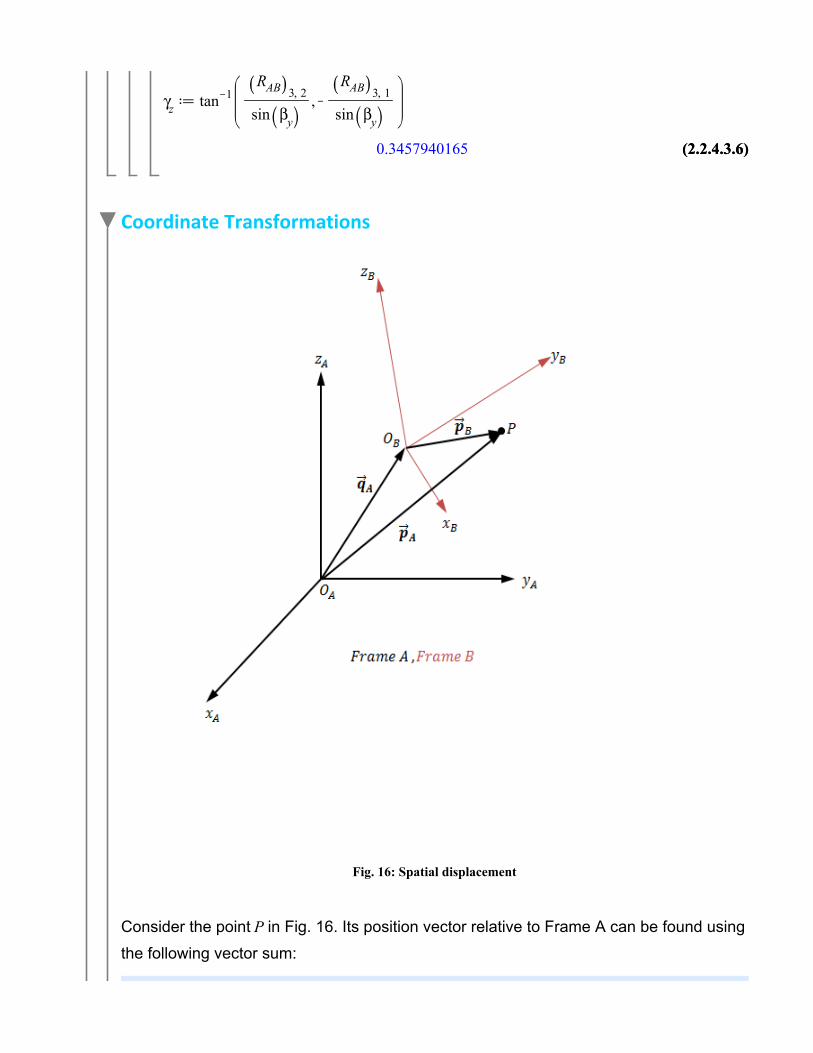
Fig. 16: Spatial displacement
Consider the point in Fig. 16. Its position vector relative to Frame A can be found using
the following vector sum:
... Eq. (18)
This can be written as
... Eq. (19)
where is the rotation matrix of Frame B with respect to Frame A, is the position
vector of the origin of Frame B with respect to Frame A and is the position vector
of point with respect to Frame B. This is the general transformation of a position vector
from one frame to another. To make this equation more compact, the concepts of
homogeneous coordinates and homogeneous transformation matrix are introduced.
Homogeneous Transformation Matrix
The homogeneous transformation matrix is a 4x4 matrix that is defined for mapping a
position vector from one coordinate system to another. The matrix has the following
form
... Eq. (20)
Using this matrix we can rewrite Eq. (19) as
... Eq. (21)
Here and are 4 dimensional vectors that are called
homogeneous position vectors. They simply allow for the transformations to be written
and computed in a compact form. The first three elements of a homogeneous position
vector are the components of the corresponding position vector and the fourth
element is 1. By introducing a new notation to represent homogeneous vectors, Eq.
(21) can be written as
... Eq. (22)
Inverse of a Homogeneous Transformation Operator
... Eq. (23)
Successive Transformations
Fig. 17: Three reference frames
Consider the point in Fig. (17). The homogeneous position vector of point with
respect of Frame C is . To find the position vector of the point with respect to Frame
B, the following transformation is required
... Eq. (24)
Similarly, to find the position vector of point with respect to Frame C, the following
transformations are required
... Eq. (25)
This means that
... Eq. (26)
These steps show that multiplying the transformation matrices is equivalent to taking
successive transformations. The following is the transformation matrix for two
successive transformations.
... Eq. (27)
Example 2: Robot Arm (with MapleSim)
Fig. 18: Three segment robotic arm
Problem Statement: A robot arm (see Fig. 18), consisting of three segments, has end
fixed to the ground and end free to perform tasks. The arm has three joints and each one
has its own frame of reference. The orientation of Frame B with respect to Frame A is
, the position vector of the origin of Frame B with respect to Frame A
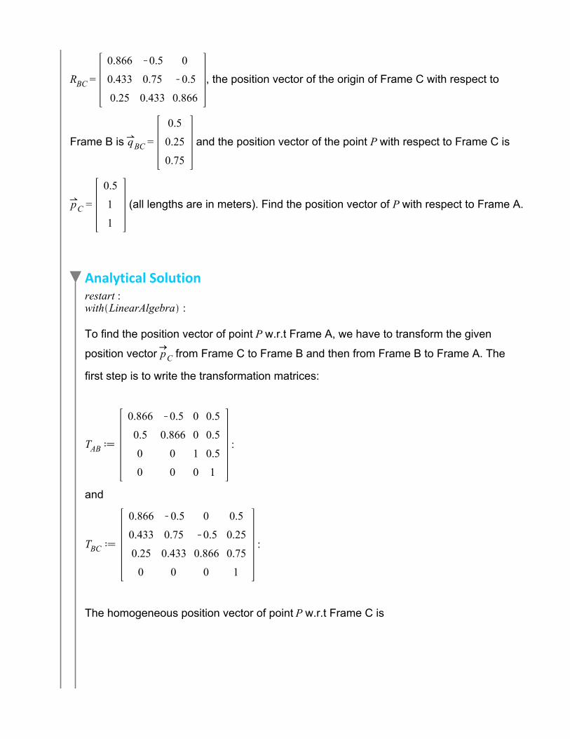
is , the orientation of Frame C with respect to Frame B is
, the position vector of the origin of Frame C with respect to
Frame B is and the position vector of the point with respect to Frame C is
(all lengths are in meters). Find the position vector of with respect to Frame A.
Analytical Solution
To find the position vector of point w.r.t Frame A, we have to transform the given
position vector from Frame C to Frame B and then from Frame B to Frame A. The
first step is to write the transformation matrices:
and
The homogeneous position vector of point w.r.t Frame C is
(3.1.1)(3.1.1)
1. 1.
Now, these three matrices can be multiplied to obtain the homogeneous position vector
of point w.r.t Frame A.
Therefore, the position vector of point with respect to Frame A is (m).
Solution with MapleSim
Constructing the model
Step 1: Insert component
Drag the following components into the workspace:
Table 3: Components and locations
Component Location
Multibody > Bodies and
Frames
2. 2.
(3 required)
Multibody > Bodies and
Frames
(3 required)
Multibody > Visualization
Multibody > Sensors
Copy the Axes subsystem created in the Cascade Rotations subsection and
paste it twice into the workspace (or follow the steps provided in that subsection
to create the subsystem again).
Step 2: Connect components
Connect the subsystems as shown in the following diagram.
3. 3.
4. 4.
2. 2.
1. 1.
5. 5.
Fig. 19: Robot arm component diagram
Step 3: Set the component parameters
Click the Rigid Body Frame component connected to the Fixed Frame
component and enter for the x,y,z offset ( ).
Select Rotation Matrix in the drop-down menu for TypeR and enter
for [R]. This is the transpose (and the inverse) of . A Rigid
Body Frame component provides a frame of reference (frame_b) that has a
fixed displacement ( ) and a fixed orientation ( [R] ) relative to another frame
of reference (frame_a).
Click the next Rigid Body Frame component in the chain and enter for
the x,y,z offset ( ).
Select Rotation Matrix in the drop-down menu for TypeR and enter
for [R]. This is the transpose (and the inverse) of .
Click the third Rigid Body Component and enter
3. 3.
4. 4.
1. 1.
5. 5.
2. 2.
6. 6.
for the x,y,z offset (
).
Click the Absolute Translation sensor component and select Inertial in the
Frame drop-down menu. Frame A is the ground frame and coincides with the
inertial frame (to measure the position of the point relative to another frame a
Relative Translation sensor component can be used).
Step 4: Run the Simulation
Attach a Probe to the r port of the Absolute Translation Sensor component.
Click the Probe and select 1, 2, and 3 in the Inspector Pane.
Change the Simulation duration ( ) in the Settings Pane to 0.1 s or any other
small value. Since there is no motion involved the duration of the simulation is
not important.
Click Run Simulation ( ).
This simulation outputs three plots that give the position of the point with respect to
Frame A (see Fig. 20). Since the model does not move, the plots will show horizontal
lines. The results of these plots match the results obtained analytically.
Fig. 20: Simulation results
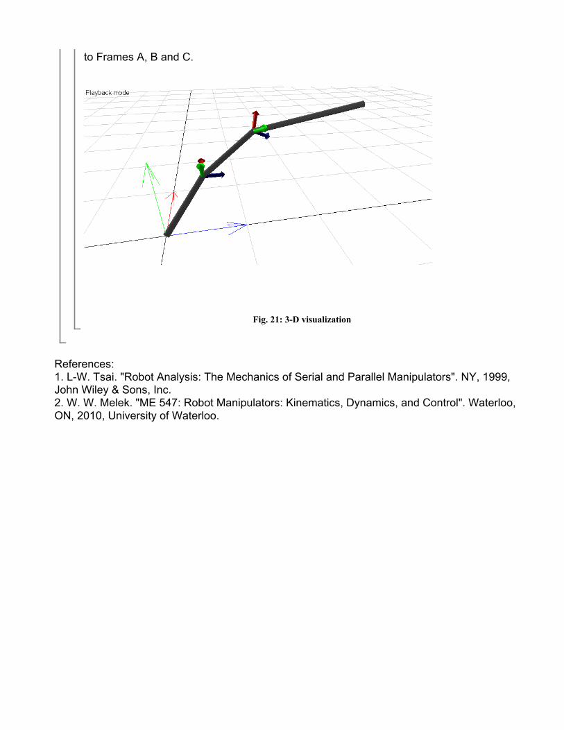
Fig. 21 shows the 3-D visualization of the robot arm. The three sets of axes correspond
5. 5.
to Frames A, B and C.
Fig. 21: 3-D visualization
References:1. L-W. Tsai. "Robot Analysis: The Mechanics of Serial and Parallel Manipulators". NY, 1999, John Wiley & Sons, Inc.2. W. W. Melek. "ME 547: Robot Manipulators: Kinematics, Dynamics, and Control". Waterloo, ON, 2010, University of Waterloo.