1

Robot Perception Continued

Visual Perception

  Visual Odometry   Reconstruction   Recognition

CS 685 11

Range Sensing strategies

  Active range sensors   Ultrasound   Laser range sensor

Slides adopted from Siegwart and Nourbakhsh

Range Sensors (time of flight) (1)

  Range distance measurement: called range sensors   Range information:

  key element for localization and environment modeling

  Ultrasonic sensors as well as laser range sensors make use of propagation speed of sound or electromagnetic waves respectively. The traveled distance of a sound or electromagnetic wave is given by

  d = c . t   Where

  d = distance traveled (usually round-trip)   c = speed of wave propagation   t = time of flight.

4.1.6

Range Sensors (time of flight) (2)

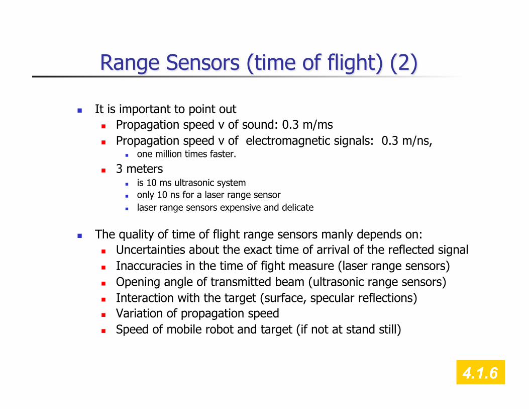
  It is important to point out   Propagation speed v of sound: 0.3 m/ms   Propagation speed v of electromagnetic signals: 0.3 m/ns,

  one million times faster.

  3 meters   is 10 ms ultrasonic system   only 10 ns for a laser range sensor   laser range sensors expensive and delicate

  The quality of time of flight range sensors manly depends on:   Uncertainties about the exact time of arrival of the reflected signal   Inaccuracies in the time of fight measure (laser range sensors)   Opening angle of transmitted beam (ultrasonic range sensors)   Interaction with the target (surface, specular reflections)   Variation of propagation speed   Speed of mobile robot and target (if not at stand still)

4.1.6

Ultrasonic Sensor (sound) (1)

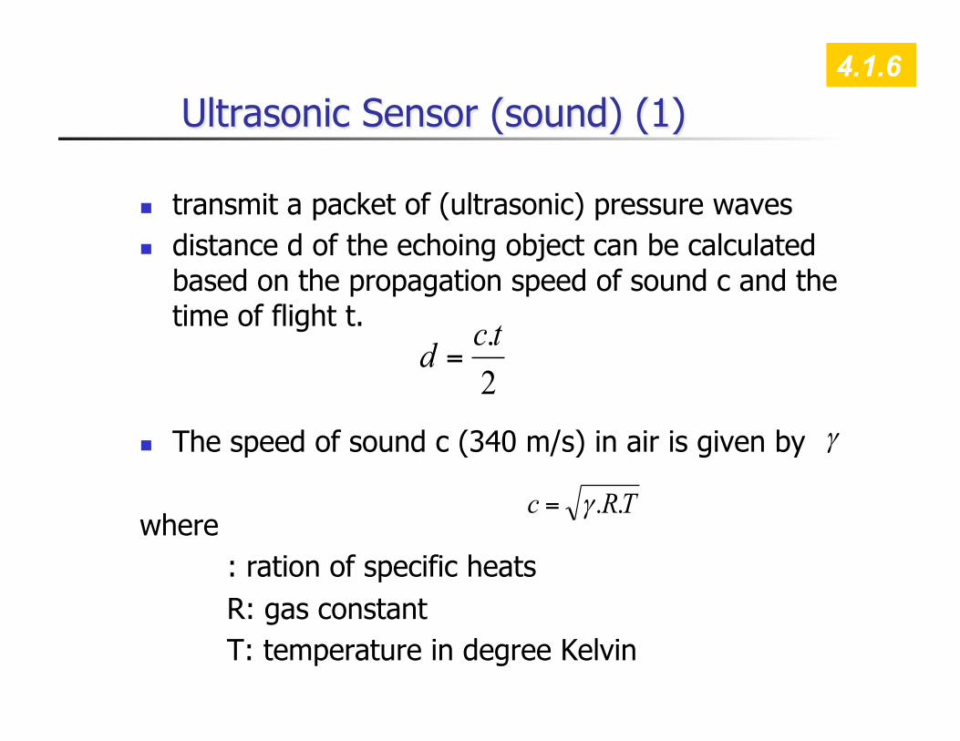
  transmit a packet of (ultrasonic) pressure waves   distance d of the echoing object can be calculated

based on the propagation speed of sound c and the time of flight t.

  The speed of sound c (340 m/s) in air is given by

where : ration of specific heats R: gas constant T: temperature in degree Kelvin

TRc ..γ=

2.tcd =

γ

4.1.6

Ultrasonic Sensor (sound) (3)

  typically a frequency: 40 - 180 kHz   generation of sound wave: piezo transducer

  transmitter and receiver separated or not separated   sound beam propagates in a cone like manner

  opening angles around 20 to 40 degrees   regions of constant depth   segments of an arc (sphere for 3D)   Effective range 12cm, 5m   Accuracy between 98-99%

Typical intensity distribution of a ultrasonic sensor

-30°

-60°

0°30°

60°

Amplitude [dB]

measurement cone

4.1.6

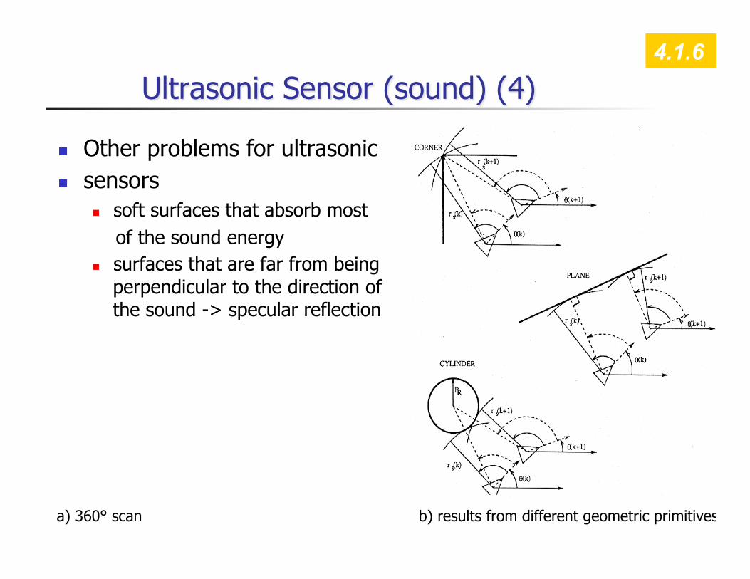
Ultrasonic Sensor (sound) (4)

  Other problems for ultrasonic   sensors

  soft surfaces that absorb most of the sound energy   surfaces that are far from being

perpendicular to the direction of the sound -> specular reflection

a) 360° scan b) results from different geometric primitives

4.1.6

Sources of Error

  Opening angle   Crosstalk   Specular reflection

Slide adopted from C. Stachniss

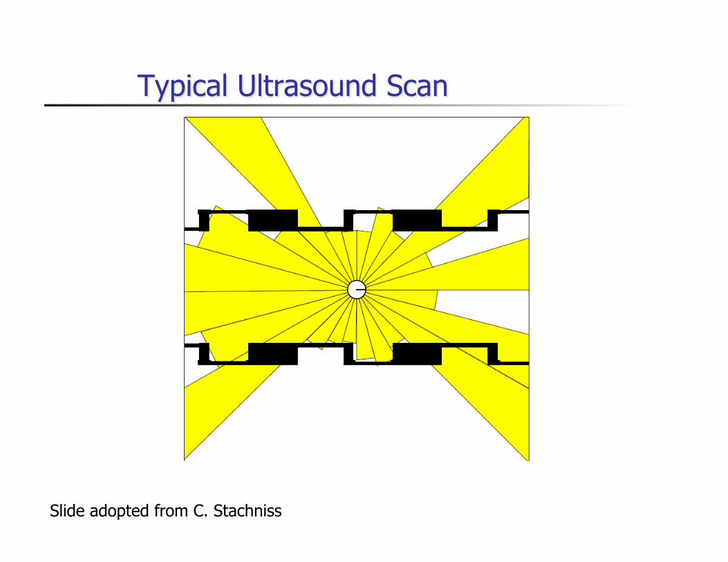
Typical Ultrasound Scan

Slide adopted from C. Stachniss

Parallel Operation

  Given a 15 degrees opening angle, 24 sensors are needed to cover the whole 360 degrees area around the robot.

  Let the maximum range we are interested in be 10m.

  The time of flight then is 2*10/330 s=0.06 s

  A complete scan requires 1.45 s

  To allow frequent updates (necessary for high speed) the sensors have to be fired in parallel.

  This increases the risk of crosstalk

Slide adopted from C. Stachniss

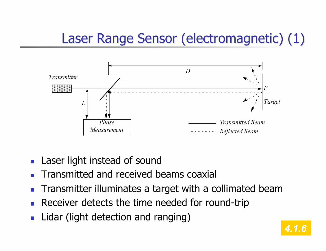
Laser Range Sensor (electromagnetic) (1)

  Laser light instead of sound   Transmitted and received beams coaxial   Transmitter illuminates a target with a collimated beam   Receiver detects the time needed for round-trip   Lidar (light detection and ranging)

PhaseMeasurement

Target

D

L

Transmitter

Transmitted BeamReflected Beam

P

4.1.6

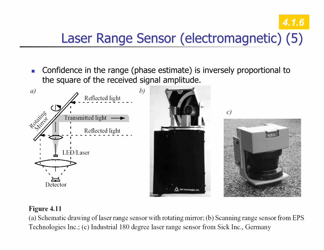
Laser Range Sensor (electromagnetic) (5)

  Confidence in the range (phase estimate) is inversely proportional to the square of the received signal amplitude.   Hence dark, distant objects will not produce such good range

estimated as closer brighter objects …

4.1.6

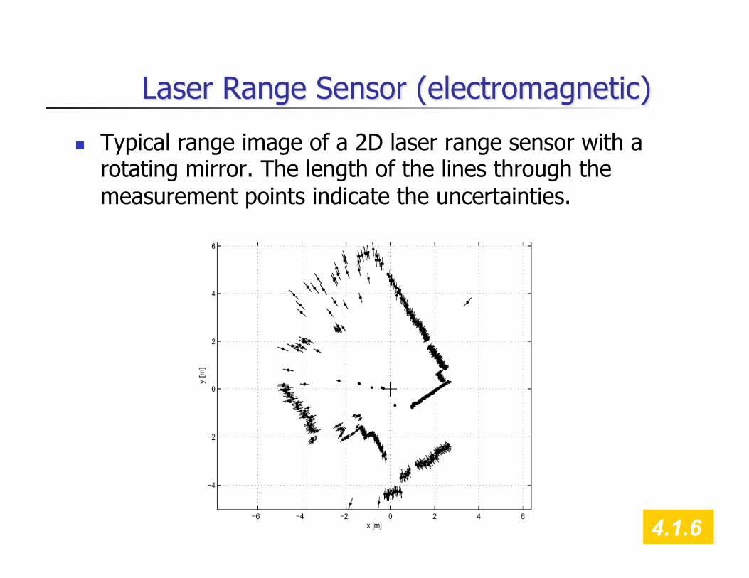
Laser Range Sensor (electromagnetic)

  Typical range image of a 2D laser range sensor with a rotating mirror. The length of the lines through the measurement points indicate the uncertainties.

4.1.6

29

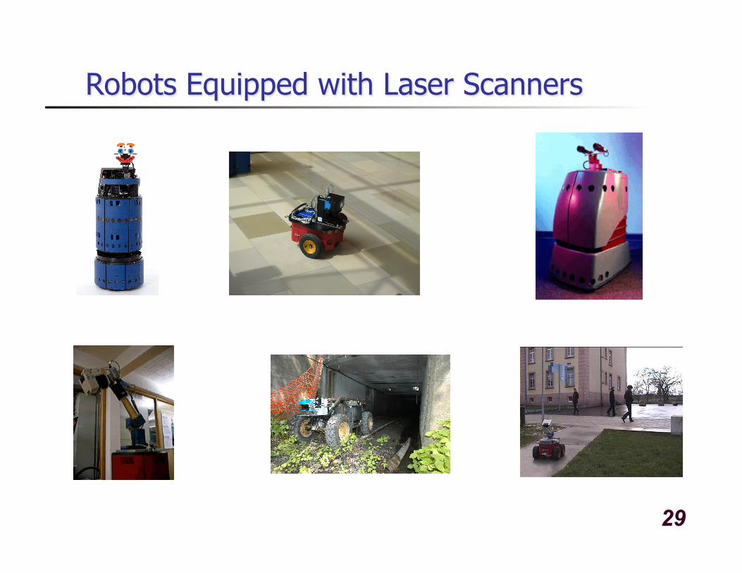
Robots Equipped with Laser Scanners

30

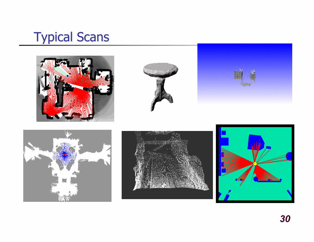
Typical Scans

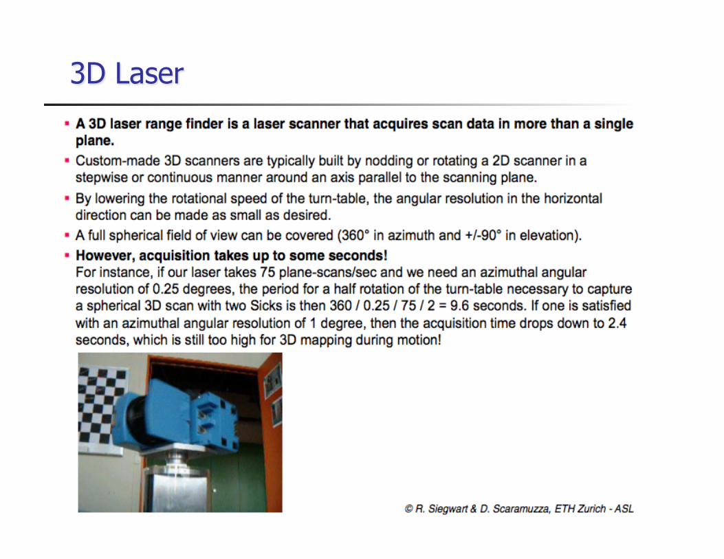
3D Laser

3D Laser

Heading Sensors

  Heading sensors can be proprioceptive (gyroscope, inclinometer) or exteroceptive (compass).

  Used to determine the robots orientation and inclination.

  Allow, together with an appropriate velocity information, to integrate the movement to an position estimate.   This procedure is called dead reckoning (ship navigation)

4.1.4

Compass

  Since over 2000 B.C.   when Chinese suspended a piece of naturally magnetite

from a silk thread and used it to guide a chariot over land.   Magnetic field on earth

  absolute measure for orientation.   Large variety of solutions to measure the earth magnetic field

  mechanical magnetic compass   direct measure of the magnetic field (Hall-effect,

magnetoresistive sensors)   Major drawback

  weakness of the earth field   easily disturbed by magnetic objects or other sources   not feasible for indoor environments

4.1.4

Gyroscope

  Heading sensors, that keep the orientation to a fixed frame   absolute measure for the heading of a mobile system.

  Two categories, the mechanical and the optical gyroscopes   Mechanical Gyroscopes

  Standard gyro   Rated gyro

  Optical Gyroscopes   Rated gyro

4.1.4

Global Positioning System (GPS) (1)   Developed for military use   Recently it became accessible for commercial applications   24 satellites (including three spares) orbiting the earth every

12 hours at a height of 20.190 km.   Four satellites are located in each of six planes inclined 55

degrees with respect to the plane of the earth’s equators   Location of any GPS receiver is determined through a time

of flight measurement

  Technical challenges:   Time synchronization between the individual satellites and

the GPS receiver   Real time update of the exact location of the satellites   Precise measurement of the time of flight   Interferences with other signals

4.1.5

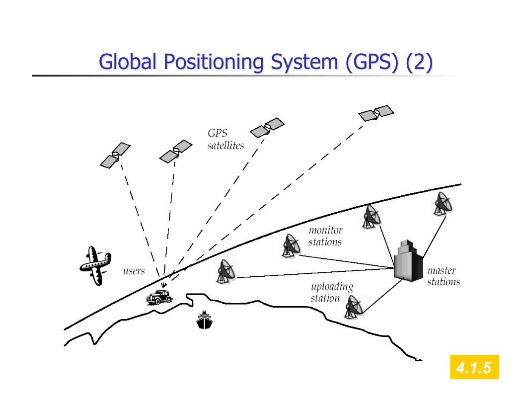
Global Positioning System (GPS) (2)

4.1.5

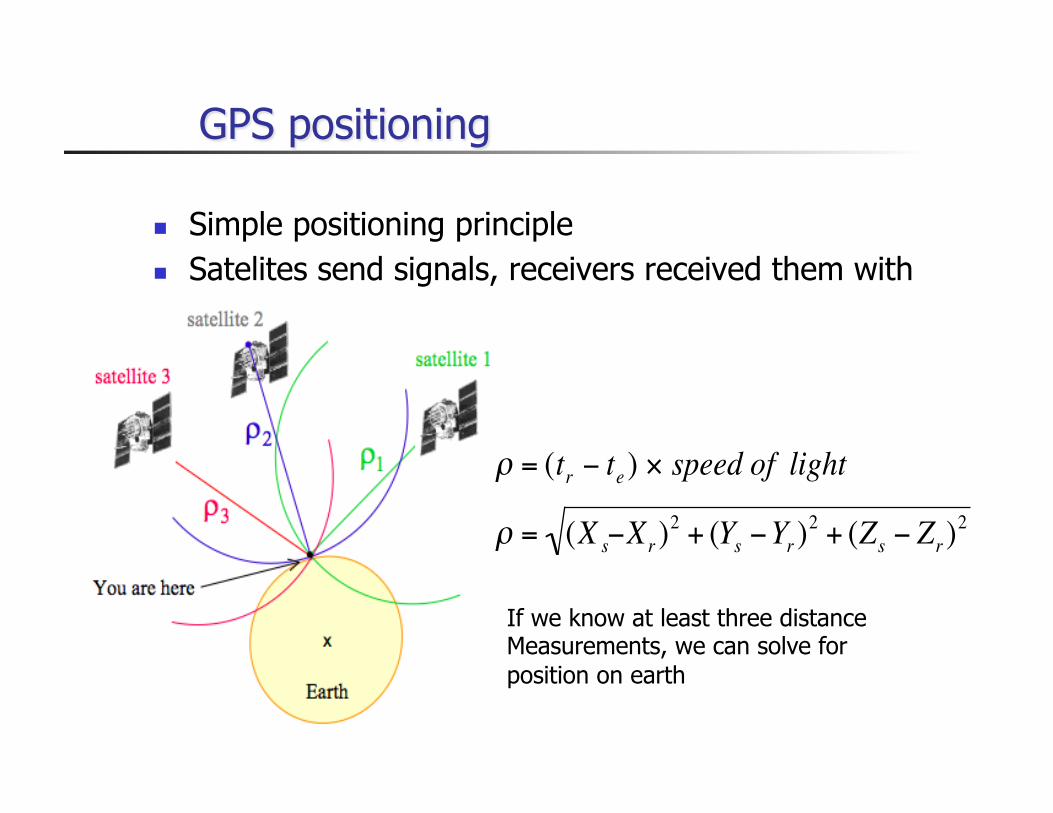
GPS positioning

  Simple positioning principle   Satelites send signals, receivers received them with

delay

€

ρ = (tr − te ) × speed of light

€

ρ = (X s−Xr )2 + (Ys −Yr )

2 + (Zs − Zr )2

If we know at least three distance Measurements, we can solve for position on earth

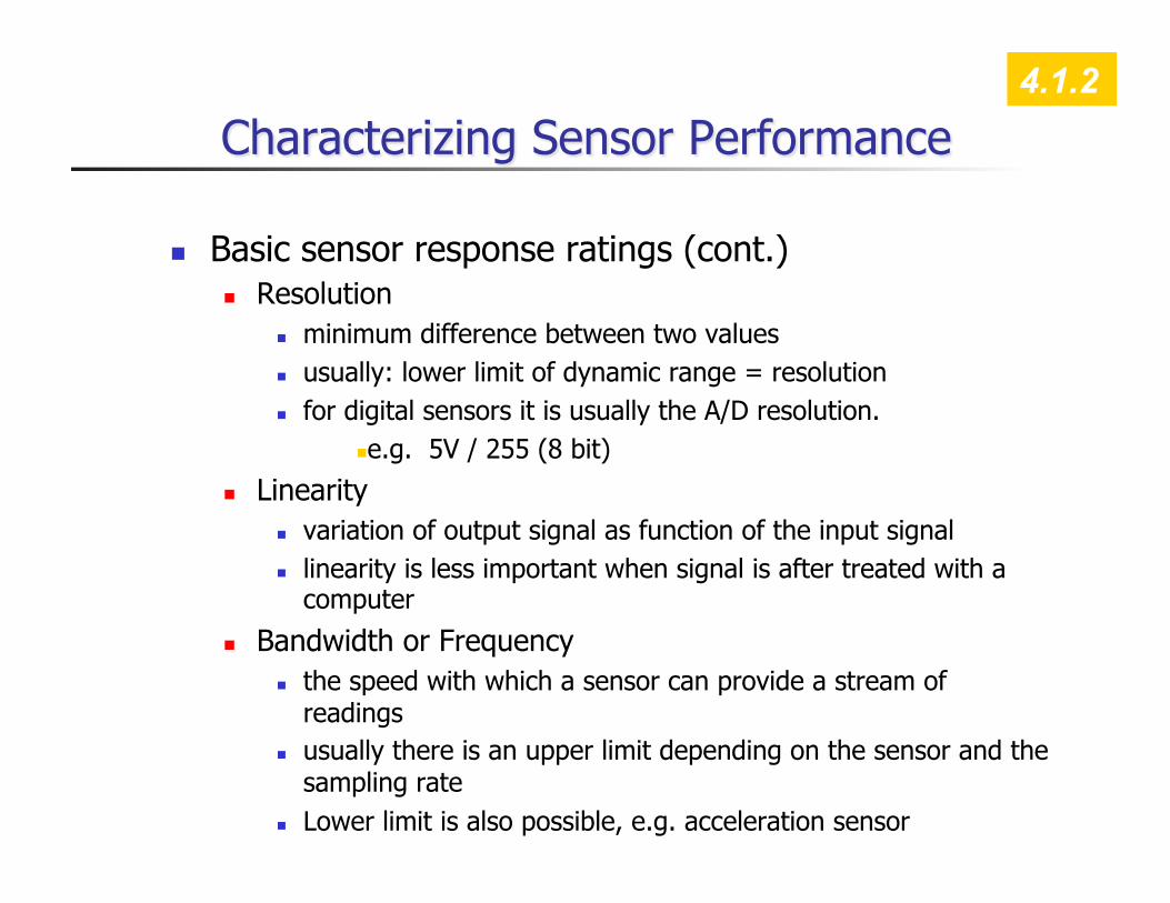
Characterizing Sensor Performance

  Basic sensor response ratings (cont.)   Resolution

  minimum difference between two values   usually: lower limit of dynamic range = resolution   for digital sensors it is usually the A/D resolution.

 e.g. 5V / 255 (8 bit)

  Linearity   variation of output signal as function of the input signal   linearity is less important when signal is after treated with a

computer

  Bandwidth or Frequency   the speed with which a sensor can provide a stream of

readings   usually there is an upper limit depending on the sensor and the

sampling rate   Lower limit is also possible, e.g. acceleration sensor

4.1.2

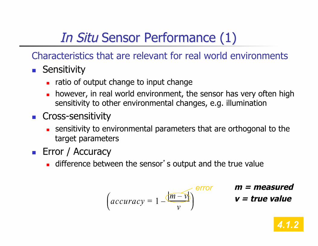
In Situ Sensor Performance (1) Characteristics that are relevant for real world environments   Sensitivity

  ratio of output change to input change   however, in real world environment, the sensor has very often high

sensitivity to other environmental changes, e.g. illumination

  Cross-sensitivity   sensitivity to environmental parameters that are orthogonal to the

target parameters

  Error / Accuracy   difference between the sensor’s output and the true value

m = measured v = true value

error

4.1.2

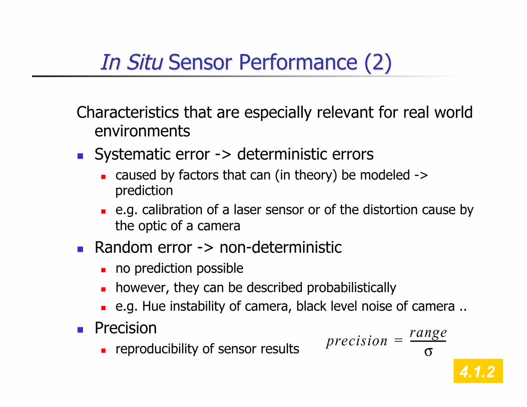
In Situ Sensor Performance (2)

Characteristics that are especially relevant for real world environments

  Systematic error -> deterministic errors   caused by factors that can (in theory) be modeled ->

prediction   e.g. calibration of a laser sensor or of the distortion cause by

the optic of a camera

  Random error -> non-deterministic   no prediction possible   however, they can be described probabilistically   e.g. Hue instability of camera, black level noise of camera ..

  Precision   reproducibility of sensor results

4.1.2

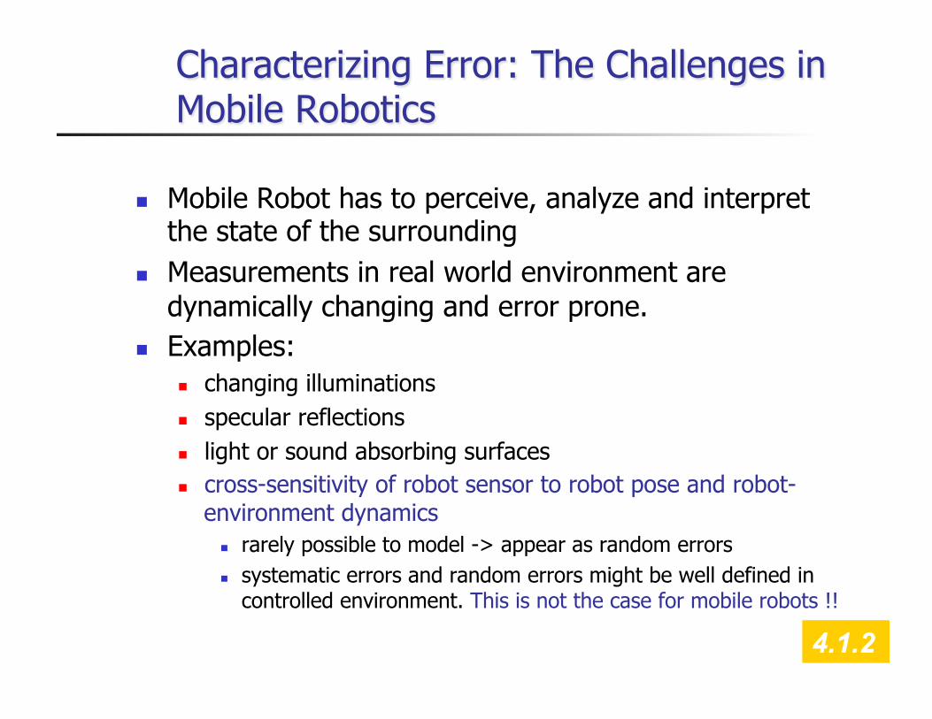
Characterizing Error: The Challenges in Mobile Robotics

  Mobile Robot has to perceive, analyze and interpret the state of the surrounding

  Measurements in real world environment are dynamically changing and error prone.

  Examples:   changing illuminations   specular reflections   light or sound absorbing surfaces   cross-sensitivity of robot sensor to robot pose and robot-

environment dynamics   rarely possible to model -> appear as random errors   systematic errors and random errors might be well defined in

controlled environment. This is not the case for mobile robots !!

4.1.2

Multi-Modal Error Distributions: The Challenges in …

  Behavior of sensors modeled by probability distribution (random errors)   usually very little knowledge about the causes of random

errors   often probability distribution is assumed to be symmetric or

even Gaussian   however, it is important to realize how wrong this can be!   Examples:

  Sonar (ultrasonic) sensor might overestimate the distance in real environment and is therefore not symmetric

- Thus the sonar sensor might be best modeled by two modes: - mode for the case that the signal returns directly - mode for the case that the signals returns after multi-path reflections.

  Stereo vision system might correlate to images incorrectly, thus causing results that make no sense at all 4.1.2