Robotica · Robotica, Systems Control,”

Roboticahttp://journals.cambridge.org/ROB

Additional services for Robotica:

Email alerts: Click hereSubscriptions: Click hereCommercial reprints: Click hereTerms of use : Click here

Distributed formation control of networked mobile robots in environments with obstacles

Whye Leon Seng, Jan Carlo Barca and Y. Ahmet Şekercioğlu

Robotica / Volume 34 / Issue 06 / June 2016, pp 1403 - 1415DOI: 10.1017/S0263574714002380, Published online: 15 October 2014

Link to this article: http://journals.cambridge.org/abstract_S0263574714002380

How to cite this article:Whye Leon Seng, Jan Carlo Barca and Y. Ahmet Şekercioğlu (2016). Distributed formation control of networked mobilerobots in environments with obstacles. Robotica, 34, pp 1403-1415 doi:10.1017/S0263574714002380

Request Permissions : Click here

Downloaded from http://journals.cambridge.org/ROB, IP address: 195.83.155.55 on 03 May 2016

http://journals.cambridge.org Downloaded: 03 May 2016 IP address: 195.83.155.55

Robotica (2016) volume 34, pp. 1403–1415. © Cambridge University Press 2014doi:10.1017/S0263574714002380

Distributed formation control of networked mobilerobots in environments with obstaclesWhye Leon Seng†∗, Jan Carlo Barca‡ andY. Ahmet Sekercioglu††Department of Electrical and Computer Systems Engineering, Monash University, Melbourne,Australia. E-mail: [email protected]‡Clayton School of Information Technology, Monash University, Melbourne, Australia.E-mail:, [email protected]

(Accepted August 18, 2014. First published online: October 15, 2014)

SUMMARYA distributed control mechanism for ground moving nonholonomic robots is proposed. It enablesa group of mobile robots to autonomously manage formation shapes while navigating throughenvironments with obstacles. The mechanism consists of two stages, with the first being formationcontrol that allows basic formation shapes to be maintained without the need of any inter-robotcommunication. It is followed by obstacle avoidance, which is designed with maintaining theformation in mind. Every robot is capable of performing basic obstacle avoidance by itself. However,to ensure that the formation shape is maintained, formation scaling is implemented. If the formationfails to hold its shape when navigating through environments with obstacles, formation morphinghas been incorporated to preserve the interconnectivity of the robots, thus reducing the possibility oflosing robots from the formation.

The algorithm has been implemented on a nonholonomic multi-robot system for empiricalanalysis. Experimental results demonstrate formations completing an obstacle course within 12 swith zero collisions. Furthermore, the system is capable of withstanding up to 25% sensor noise.

KEYWORDS: Robot networks; Formation control; Swarm robotics.

1. IntroductionIn recent years there has been an increasing interest in automated control and coordination of multirobot systems. The advancement in technology and increasing safety awareness have pushed for thedevelopment of such systems, particularly in tasks where human lives are at stake such as in searchand rescue operations, environmental sensing, or reconnaissance. Existing solutions are often costly,require nearly continuous monitoring from a base station, and/or only deploy small numbers of robotswith limited geographical coverage, therefore severely reducing their effectiveness. One solution tothis problem is to introduce a distributed swarm-based system. With multiple, structurally identicallesser robots working as a group, a swarm is capable of performing tasks beyond the capabilities ofa single robot. Such a system would significantly drive down the cost of deployment as each robotonly requires the most basic sensor equipment. It also allows the system to be scalable and possessself-repairing abilities should several robots within the swarm fail. This translates to a much higherreliability and reduced risk of mission failure.1

Several investigations on this issue have been considered.2, 3 Shao et al.2 consider a one-leader constraint formation control, which produces a non-rigid formation control graph. Itemploys adjacency and parameter matrices which simplifies the definitions of local leader-followerrelationships and the overall formation shape. However, non-rigid formation control does not allow theformation shape to be maintained as the formation moves. The obstacle avoidance method considered

* Corresponding author. E-mail: [email protected]

http://journals.cambridge.org


1404 Distributed formation control

is also insufficient in dealing with more complex obstacles and may cause robots to be trapped behindobstacles. Formation control with both one-leader and two-leaders constraints was presented in.3

Their work focuses on how transitions between formations can be realized via a transition matrix.How control graphs can be classified on the basis of the number of followers with one and two leadersis also investigated. However, as in,2 they do not explain how one can select ideal formation shapesin environments with obstacles.

We have also looked into several obstacle avoidance methods in this research. Obstacles areregarded as virtual leaders in,4, 5 forcing robots to maintain a distance from obstacles, in a mannersimilar to how the robots maintain formation shapes by keeping a distance from their Local Leaders(LL). The downside is that the formation may no longer be rigid as robots may have to sever theconnections with their LLs in order to apply the distance constraints for the obstacles. A behavior-based formation control is proposed in,6 where a swarm of robots navigates about obstacles simplyby rotating and scaling the overall formation. However, rotating a formation of nonholonomic robotscan be time consuming and inefficient. Kuppan et al. proposes that on detection of an obstacle,the robot is elected as the temporary Formation Leader (FL), allowing it to steer the formationaway from the obstacle.7 The drawback with this approach is that selecting the temporary leaderscomplicates the control process significantly when the formation detects multiple obstacles fromdifferent directions. A semi-rigid obstacle avoidance approach is presented in,8 where the follower isallowed to vary the angle constraint from the leader in order to steer clear of obstacles. The downsidewith this approach is that robots are unable to tackle obstacles efficiently when they have two or moreLLs, with multiple distance constraints to abide by. Another technique is to utilize potential fieldswhere interaction between robots and obstacles are represented by repulsive and attractive forces.9–12

However, the algorithms only considered the distances of the obstacles in determining the magnitudeof repulsive forces, which may cause the robots to slow down excessively even when the obstaclesare not necessarily blocking them.

The common problem with the techniques discussed above is that they have not been implementedon real robots,1–6, 9–12 where issues such as sensor noise and kinematics must be considered in orderto accurately evaluate the performance of control mechanisms for the robots. The second problemis the negligence of additional constraints posed by nonholonomic robots. The solutions to obstacleavoidance are presented as net force vectors in,10–12 indicating the instantaneous velocity that arobot should take. However, nonholonomic robots are not capable of switching from one state toanother arbitrary one immediately. In our work, we have explicitly detailed the algorithm and itsoutput in meaningful physical terms such as velocities and angular velocities, which can be includedeffortlessly in the control systems of existing robots. We have implemented the control mechanismson the eBug multi robot system13 to properly evaluate the algorithm. Parameters for the algorithmwere determined more conservatively to minimize the impact of issues such as sensor noise, wheelslippage and a noisy wireless channel.

In Section 2, the proposed formation control method is described. Section 3 introduces theimplemented obstacle avoidance techniques, followed by a discussion of formation rebuilding inSection 4. The performance of the algorithm measured from conducted experiments is discussed inSection 5. Section 6 concludes the paper as well as the possible future research work that can bedone.

2. Formation ControlThe proposed formation control algorithm is an improvement on the work presented in.14 It employsgraph theory based formation structures that branches out from a FL to Follower Robots (FR), whichare each assigned LLs according to their allocated positions in the formation, or Formation Position(FP).

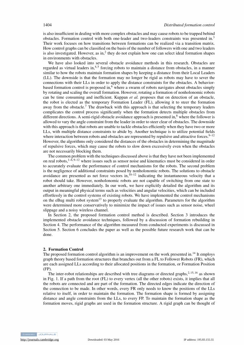
The inter-robot relationships are described with tree diagrams or directed graphs,2, 15, 16 as shownin Fig. 1. If a path from the root (FL) to every vertex (all the other robots) exists, it implies that allthe robots are connected and are part of the formation. The directed edges indicate the direction ofthe connection to be made. In other words, every FR only needs to know the positions of the LLsrelative to itself, in order to maintain the formation. The formation shape is formed by assigningdistance and angle constraints from the LLs, to every FP. To maintain the formation shape as theformation moves, rigid graphs are used in the formation structure. A rigid graph can be thought of



Distributed formation control 1405

Fig. 1. Inter-robot relationships are represented as a directed graph, where the directed edges go from thefollower robots to their local leaders.

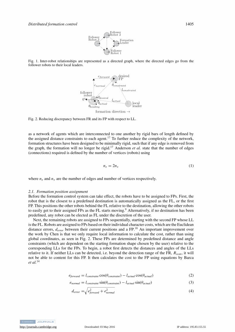
Fig. 2. Reducing discrepancy between FR and its FP with respect to LL.

as a network of agents which are interconnected to one another by rigid bars of length defined bythe assigned distance constraints to each agent.17 To further reduce the complexity of the network,formation structures have been designed to be minimally rigid, such that if any edge is removed fromthe graph, the formation will no longer be rigid.17 Anderson et al. state that the number of edges(connections) required is defined by the number of vertices (robots) using

ne = 2nv (1)

where ne and nv are the number of edges and number of vertices respectively.

2.1. Formation position assignmentBefore the formation control system can take effect, the robots have to be assigned to FPs. First, therobot that is the closest to a predefined destination is automatically assigned as the FL, or the firstFP. This positions the other robots behind the FL relative to the destination, allowing the other robotsto easily get to their assigned FPs as the FL starts moving.9 Alternatively, if no destination has beenpredefined, any robot can be elected as FL under the discretion of the user.

Next, the remaining robots are assigned to FPs sequentially, starting with the second FP whose LLis the FL. Robots are assigned to FPs based on their individual character costs, which are the Euclideandistance errors, derror between their current positions and a FP.18 An important improvement overthe work by Chen is that we only require local information to calculate the cost, rather than usingglobal coordinates, as seen in Fig. 2. These FPs are determined by predefined distance and angleconstraints (which are dependent on the starting formation shape chosen by the user) relative to thecorresponding LLs for the FPs. To begin, a robot first detects the distances and angles of the LLsrelative to it. If neither LLs can be detected, i.e. beyond the detection range of the FR, Rscan, it willnot be able to content for this FP. It then calculates the cost to the FP using equations by Barcaet al.14

eforward = lconstraint cos(θconstraint) − lactual cos(θactual) (2)

enormal = lconstraint sin(θconstraint) − lactual sin(θactual) (3)

derror =√

e2forward + e2

normal (4)




where

eforward : distance error in direction of formation movement,enormal : distance error in direction perpendicular to formation movement,lconstraint : required distance between robot and LL for this FP,lactual : actual distance between robot and LL for this FP,θconstraint : required angle from robot to LL for this FP,θactual : actual angle from robot to LL for this FP, andderror : Euclidean distance error from robot to this FP.

Note that the angles under the formation control section are all measured with respect to the oppositedirection of where the formation is heading. This process is performed by every robot that has notbeen assigned a FP and the FP is finally assigned to the robot with the lowest derror for that FP.If a FP requires two LLs, the robots content for the FP with the average derror from both LLs.The aforementioned steps are then repeated for the next FP, with its associated distance and angleconstraints. The assignments of FP are recorded in an adjacency matrix which describes the leader-follower relationships, and a parameter matrix which stores the assigned constraints. These matricesare described in detail by.2, 3

2.2. Control systemTo maintain the shape of the formation as it moves, the FRs first calculates the eforward and enormal totheir FPs (Eqs. (2) and (3)). These values are then used by a Velocity Controller (VC) and an AngularVelocity Controller (AVC) to calculate the required responses for reducing derror between a FR andits FP.

2.2.1. Velocity controller. Velocities are calculated with a non-linear controller

v ={

Vleader log10(eforward + 1) cos(θdesired − θheading) if eforward ≥ 0Vleader log10(−eforward + 1) cos(θdesired − θheading) otherwise

(5)

where

v : velocity output,Vleader : maximum velocity of formation leader,eforward : distance error in direction of formation movement,θdesired : angle of FP measured from FR, andθheading : heading angle of FR,

to provide rapid convergence towards the desired FP. A cosine multiplier which considers the angle thatthe FR faces is added to reduce unnecessary movements in the direction perpendicular to formationmovement.

2.2.2. Angular velocity controller. The AVC has two states, which are

ω ={

Kωα if derror > Rdzone

Kω

(β − (β − α) derror

Rdzone

)otherwise

(6)

with

α = θdesired − θheading (7)

β = 180◦ − θheading (8)




where

θdesired : angle from FR to its FP,θheading : heading angle of FR,ω : angular velocity output,Kω : angular velocity constant for angular velocity control,derror : Euclidean distance error from FR to the its FP, andRdzone : radius of dead zone.

When the FR is at a Rdzone distance away from its FP, the controller steers the FR directly towardsthe FP. However, as it enters the dead zone, the controller attempts to steer the FR in the directionthat the formation is travelling in. This second state is introduced to reduce the oscillations that arisefrom the tendency of the AVC to overcorrect the heading angle of the FR when it is too close to theFP. Rdzone should only be slightly wider than the diameter of a FR as the main function of AVC is tomaintain the formation shape by keeping the FR as close to its FP as possible.

3. Obstacle AvoidanceOur implementation of obstacle avoidance technique is detailed in this section. We first describe thebasic potential field based technique, followed by how it can be used to support formation scaling andmorphing, wall following and escaping from local minima. To better explain our obstacle avoidancetechnique, we define three new zones around the robot with the radii being

Ravoid : robot starts avoiding detected obstacles,Rwf : robot takes more evasive measures such as wall-following, andRstop : robot stops entirely as the output of VC is 0.

Obstacles detected in these zones will trigger the robot to behave differently as described above. Theradii of the three zones are dependent on the size of the robot and the formation velocity to ensurethat the robots have sufficient distance to perform obstacle avoidance.

3.1. Potential field based obstacle avoidanceThe potential field based obstacle avoidance technique in9–12 considers two parameters:

1. how close the obstacle is to the robot (magnitude of repulsion force), and2. where the obstacle is located in terms of angle relative to the robot (direction of repulsion force).

These parameters result in a net repulsion force with a magnitude and a direction. However, it isdifficult to expect a nonholonomic robot to react to the repulsion force by moving in the repulseddirection instantaneously. Hence, in the following subsections, we provide the details of somemodifications to the VC and AVC that allow a nonholonomic robot to react as if there is a repulsionforce acting on it. Note that these modifications are only applied when the robot is required to performobstacle avoidance.

Obstacle avoidance is performed in two stages by considering the distance, dobject and the angle ofan object, θobject measured from the robot. The stages are:

1. Reducing velocity, and2. Turning away

An object is deemed blocking the robot if it is within Ravoid from the robot, and is in the forward 180◦arc of the robot. Forward is defined to be either at the front of the robot if the VC output is positive,or back of the robot if the VC output is negative. In the first stage, the robot only considers the closestobject and reduces its velocity with a multiplier

vmultiplier1 = 1 − e− Krise

Ravoid(dobject−Rwf ) (9)




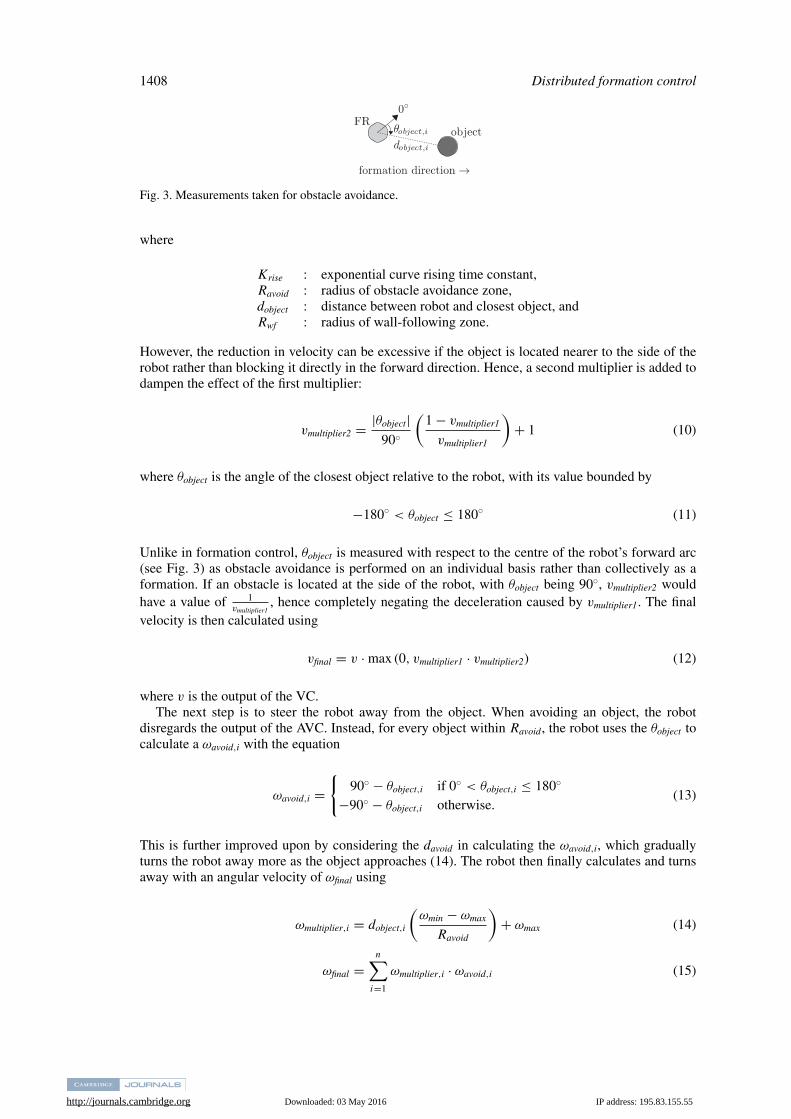
Fig. 3. Measurements taken for obstacle avoidance.

where

Krise : exponential curve rising time constant,Ravoid : radius of obstacle avoidance zone,dobject : distance between robot and closest object, andRwf : radius of wall-following zone.

However, the reduction in velocity can be excessive if the object is located nearer to the side of therobot rather than blocking it directly in the forward direction. Hence, a second multiplier is added todampen the effect of the first multiplier:

vmultiplier2 = |θobject|90◦

(1 − vmultiplier1

vmultiplier1

)+ 1 (10)

where θobject is the angle of the closest object relative to the robot, with its value bounded by

−180◦ < θobject ≤ 180◦ (11)

Unlike in formation control, θobject is measured with respect to the centre of the robot’s forward arc(see Fig. 3) as obstacle avoidance is performed on an individual basis rather than collectively as aformation. If an obstacle is located at the side of the robot, with θobject being 90◦, vmultiplier2 wouldhave a value of 1

vmultiplier1, hence completely negating the deceleration caused by vmultiplier1. The final

velocity is then calculated using

vfinal = v · max (0, vmultiplier1 · vmultiplier2) (12)

where v is the output of the VC.The next step is to steer the robot away from the object. When avoiding an object, the robot

disregards the output of the AVC. Instead, for every object within Ravoid, the robot uses the θobject tocalculate a ωavoid,i with the equation

ωavoid,i ={

90◦ − θobject,i if 0◦ < θobject,i ≤ 180◦

−90◦ − θobject,i otherwise.(13)

This is further improved upon by considering the davoid in calculating the ωavoid,i, which graduallyturns the robot away more as the object approaches (14). The robot then finally calculates and turnsaway with an angular velocity of ωfinal using

ωmultiplier,i = dobject,i

(ωmin − ωmax

Ravoid

)+ ωmax (14)

ωfinal =n∑

i=1

ωmultiplier,i · ωavoid,i (15)




where

θobject,i : angle from robot to object i,dobject,i : distance between robot and objecti,ωmin : minimum angular velocity output,ωmax : maximum angular velocity output,Ravoid : radius of obstacle avoidance zone, andωfinal : final angular velocity output.

3.2. Formation scalingFormation scaling reduces the size of the formation when confronted with external objects. Thisreduces the repulsive forces experienced by the formation and allows the robots to maintain theiroriginal formation shape for a longer period. Scaling is triggered whenever any robot detects obstacleswithin Rscan. This information is conveyed to all other robots within the formation and the distanceconstraints on the robots are continuously reduced by a factor of Kscale till a minimum value ofKscale min is reached, as expressed by

lconstraint(t + 1) ={

lconstraint(t) · Kscale if lconstraint(t)Kscale min

> lconstraint(0)

lconstraint(t) · Kscale min otherwise(16)

where

lconstraint(t) : required distance between robot and its LL at time t,Kscale : rate at which formation size scales, andKscale min : minimum formation scaling factor.

Kscale min is selected such that the robots do not get within Ravoid of other robots. When no obstaclesare detected, the process is reversed using

lconstraint(t + 1) ={

lconstraint(t)Kscale

if lconstraint(t)Kscale

< lconstraint(0)

lconstraint(0) otherwise(17)

Kscale governs the rate at which the formation size scales, hence its value is empirically determinedbased on the environment layout.

3.3. Formation morphingWhen subjected to environments with obstacles, repulsive forces from objects cause the robotsto deviate from their ideal FPs even with formation scaling. This may lead to some FRs beingdisconnected from their LLs. Formation morphing is introduced as a fail-safe should formationscaling fails to maintain the formation structure. The use of character costs and character set matrixfor every formation shape forms the basis of the implemented formation morphing solution as in.17

Whenever a robot detects an object within Ravoid, it broadcasts a signal to trigger the considerationfor formation morphing. The robots go through the same sequence as when assigning FPs (see Section2.1) multiple times for all predefined formation shapes. For every formation shape, the distance errorto ideal FPs of each robot is shared so that the total distance error for every formation shape iscalculated and recorded. The robots then select the shape that has the lowest distance error andthe new FP constraints are assigned to them. To ensure that formation morphing occurs successfullywithout the risk of losing any robots, a transition matrix is applied to the adjacency matrix as describedin.3

However, experiments show that the formation may alternate rapidly between two formation shapeswhich have similar total distance errors. Two mechanisms are introduced to prevent this issue. Thefirst mechanism is a morph timer which prevents the formation from morphing to another shape ifthe elapsed time of the morph timer is less than Tmorph. This timer resets whenever the formationsuccessfully morphs to a different shape. The second mechanism makes use of hysteresis whendeciding on a new formation shape to morph to. The formation will only morph to a new shape if the




Fig. 4. Situation where a robot may not be able to move forward.

(a) (b) (c)

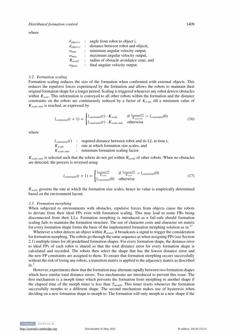
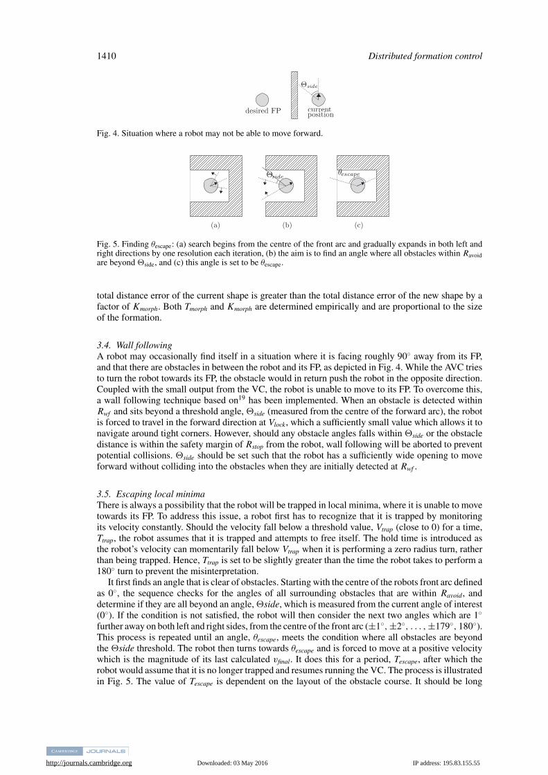
Fig. 5. Finding θescape: (a) search begins from the centre of the front arc and gradually expands in both left andright directions by one resolution each iteration, (b) the aim is to find an angle where all obstacles within Ravoidare beyond �side, and (c) this angle is set to be θescape.

total distance error of the current shape is greater than the total distance error of the new shape by afactor of Kmorph. Both Tmorph and Kmorph are determined empirically and are proportional to the sizeof the formation.

3.4. Wall followingA robot may occasionally find itself in a situation where it is facing roughly 90◦ away from its FP,and that there are obstacles in between the robot and its FP, as depicted in Fig. 4. While the AVC triesto turn the robot towards its FP, the obstacle would in return push the robot in the opposite direction.Coupled with the small output from the VC, the robot is unable to move to its FP. To overcome this,a wall following technique based on19 has been implemented. When an obstacle is detected withinRwf and sits beyond a threshold angle, �side (measured from the centre of the forward arc), the robotis forced to travel in the forward direction at Vlock, which a sufficiently small value which allows it tonavigate around tight corners. However, should any obstacle angles falls within �side or the obstacledistance is within the safety margin of Rstop from the robot, wall following will be aborted to preventpotential collisions. �side should be set such that the robot has a sufficiently wide opening to moveforward without colliding into the obstacles when they are initially detected at Rwf .

3.5. Escaping local minimaThere is always a possibility that the robot will be trapped in local minima, where it is unable to movetowards its FP. To address this issue, a robot first has to recognize that it is trapped by monitoringits velocity constantly. Should the velocity fall below a threshold value, Vtrap (close to 0) for a time,Ttrap, the robot assumes that it is trapped and attempts to free itself. The hold time is introduced asthe robot’s velocity can momentarily fall below Vtrap when it is performing a zero radius turn, ratherthan being trapped. Hence, Ttrap is set to be slightly greater than the time the robot takes to perform a180◦ turn to prevent the misinterpretation.

It first finds an angle that is clear of obstacles. Starting with the centre of the robots front arc definedas 0◦, the sequence checks for the angles of all surrounding obstacles that are within Ravoid, anddetermine if they are all beyond an angle, �side, which is measured from the current angle of interest(0◦). If the condition is not satisfied, the robot will then consider the next two angles which are 1◦further away on both left and right sides, from the centre of the front arc (±1◦, ±2◦, . . . , ±179◦, 180◦).This process is repeated until an angle, θescape, meets the condition where all obstacles are beyondthe �side threshold. The robot then turns towards θescape and is forced to move at a positive velocitywhich is the magnitude of its last calculated vfinal. It does this for a period, Tescape, after which therobot would assume that it is no longer trapped and resumes running the VC. The process is illustratedin Fig. 5. The value of Tescape is dependent on the layout of the obstacle course. It should be long




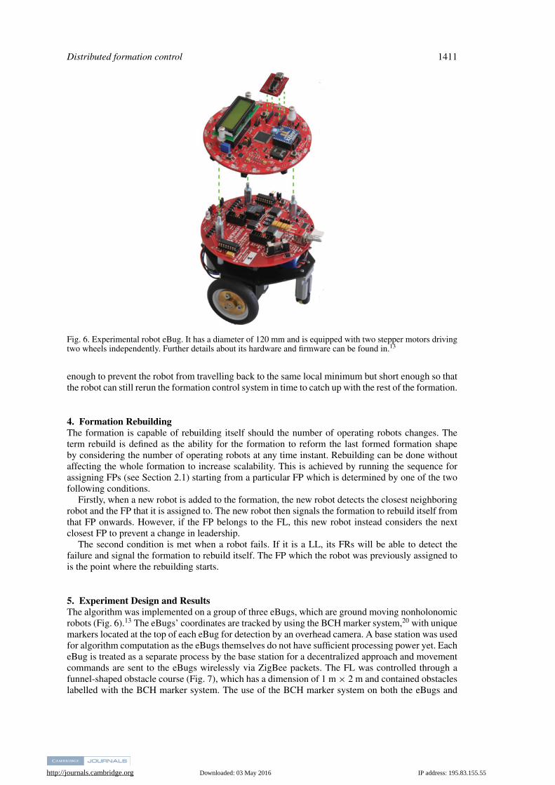
Fig. 6. Experimental robot eBug. It has a diameter of 120 mm and is equipped with two stepper motors drivingtwo wheels independently. Further details about its hardware and firmware can be found in.13

enough to prevent the robot from travelling back to the same local minimum but short enough so thatthe robot can still rerun the formation control system in time to catch up with the rest of the formation.

4. Formation RebuildingThe formation is capable of rebuilding itself should the number of operating robots changes. Theterm rebuild is defined as the ability for the formation to reform the last formed formation shapeby considering the number of operating robots at any time instant. Rebuilding can be done withoutaffecting the whole formation to increase scalability. This is achieved by running the sequence forassigning FPs (see Section 2.1) starting from a particular FP which is determined by one of the twofollowing conditions.

Firstly, when a new robot is added to the formation, the new robot detects the closest neighboringrobot and the FP that it is assigned to. The new robot then signals the formation to rebuild itself fromthat FP onwards. However, if the FP belongs to the FL, this new robot instead considers the nextclosest FP to prevent a change in leadership.

The second condition is met when a robot fails. If it is a LL, its FRs will be able to detect thefailure and signal the formation to rebuild itself. The FP which the robot was previously assigned tois the point where the rebuilding starts.

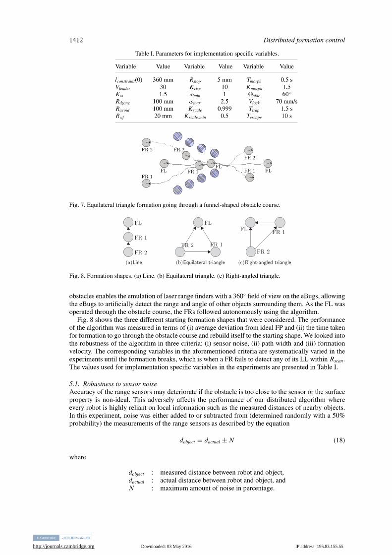
5. Experiment Design and ResultsThe algorithm was implemented on a group of three eBugs, which are ground moving nonholonomicrobots (Fig. 6).13 The eBugs’ coordinates are tracked by using the BCH marker system,20 with uniquemarkers located at the top of each eBug for detection by an overhead camera. A base station was usedfor algorithm computation as the eBugs themselves do not have sufficient processing power yet. EacheBug is treated as a separate process by the base station for a decentralized approach and movementcommands are sent to the eBugs wirelessly via ZigBee packets. The FL was controlled through afunnel-shaped obstacle course (Fig. 7), which has a dimension of 1 m × 2 m and contained obstacleslabelled with the BCH marker system. The use of the BCH marker system on both the eBugs and




Table I. Parameters for implementation specific variables.

Variable Value Variable Value Variable Value

lconstraint(0) 360 mm Rstop 5 mm Tmorph 0.5 sVleader 30 Krise 10 Kmorph 1.5Kω 1.5 ωmin 1 �side 60◦Rdzone 100 mm ωmax 2.5 Vlock 70 mm/sRavoid 100 mm Kscale 0.999 Ttrap 1.5 sRwf 20 mm Kscale min 0.5 Tescape 10 s

Fig. 7. Equilateral triangle formation going through a funnel-shaped obstacle course.

(a)Line (b)Equilateral triangle (c)Right-angled triangle

Fig. 8. Formation shapes. (a) Line. (b) Equilateral triangle. (c) Right-angled triangle.

obstacles enables the emulation of laser range finders with a 360◦ field of view on the eBugs, allowingthe eBugs to artificially detect the range and angle of other objects surrounding them. As the FL wasoperated through the obstacle course, the FRs followed autonomously using the algorithm.

Fig. 8 shows the three different starting formation shapes that were considered. The performanceof the algorithm was measured in terms of (i) average deviation from ideal FP and (ii) the time takenfor formation to go through the obstacle course and rebuild itself to the starting shape. We looked intothe robustness of the algorithm in three criteria: (i) sensor noise, (ii) path width and (iii) formationvelocity. The corresponding variables in the aforementioned criteria are systematically varied in theexperiments until the formation breaks, which is when a FR fails to detect any of its LL within Rscan.The values used for implementation specific variables in the experiments are presented in Table I.

5.1. Robustness to sensor noiseAccuracy of the range sensors may deteriorate if the obstacle is too close to the sensor or the surfaceproperty is non-ideal. This adversely affects the performance of our distributed algorithm whereevery robot is highly reliant on local information such as the measured distances of nearby objects.In this experiment, noise was either added to or subtracted from (determined randomly with a 50%probability) the measurements of the range sensors as described by the equation

dobject = dactual ± N (18)

where

dobject : measured distance between robot and object,dactual : actual distance between robot and object, andN : maximum amount of noise in percentage.




17

18

19

20

21

22

23

24

25

0 5 10 15 20 25

Pos

itio

nal E

rror

(m

m)

Noise (%)

LineEquilateral Triangle

Right Angled Triangle

(a) Average distance between actual and ideal FPs

90

100

110

120

130

140

150

160

0 5 10 15 20 25

Com

plet

ion

Tim

e (s

)

Noise (%)



(b) Time taken to complete the obstacle course

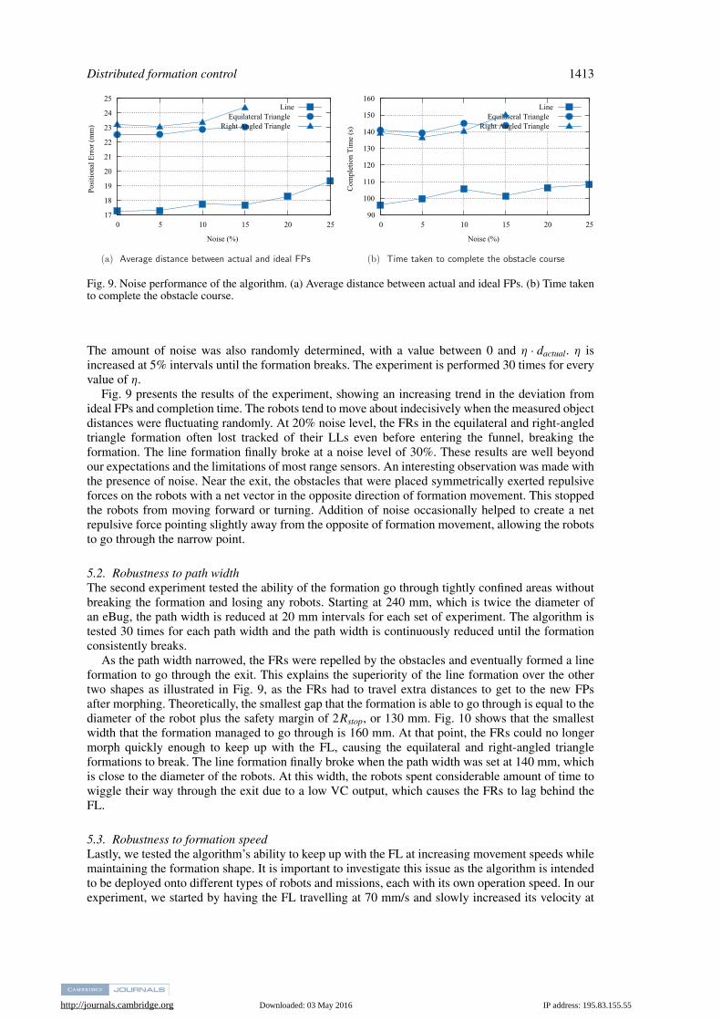
Fig. 9. Noise performance of the algorithm. (a) Average distance between actual and ideal FPs. (b) Time takento complete the obstacle course.

The amount of noise was also randomly determined, with a value between 0 and η · dactual. η isincreased at 5% intervals until the formation breaks. The experiment is performed 30 times for everyvalue of η.

Fig. 9 presents the results of the experiment, showing an increasing trend in the deviation fromideal FPs and completion time. The robots tend to move about indecisively when the measured objectdistances were fluctuating randomly. At 20% noise level, the FRs in the equilateral and right-angledtriangle formation often lost tracked of their LLs even before entering the funnel, breaking theformation. The line formation finally broke at a noise level of 30%. These results are well beyondour expectations and the limitations of most range sensors. An interesting observation was made withthe presence of noise. Near the exit, the obstacles that were placed symmetrically exerted repulsiveforces on the robots with a net vector in the opposite direction of formation movement. This stoppedthe robots from moving forward or turning. Addition of noise occasionally helped to create a netrepulsive force pointing slightly away from the opposite of formation movement, allowing the robotsto go through the narrow point.

5.2. Robustness to path widthThe second experiment tested the ability of the formation go through tightly confined areas withoutbreaking the formation and losing any robots. Starting at 240 mm, which is twice the diameter ofan eBug, the path width is reduced at 20 mm intervals for each set of experiment. The algorithm istested 30 times for each path width and the path width is continuously reduced until the formationconsistently breaks.

As the path width narrowed, the FRs were repelled by the obstacles and eventually formed a lineformation to go through the exit. This explains the superiority of the line formation over the othertwo shapes as illustrated in Fig. 9, as the FRs had to travel extra distances to get to the new FPsafter morphing. Theoretically, the smallest gap that the formation is able to go through is equal to thediameter of the robot plus the safety margin of 2Rstop, or 130 mm. Fig. 10 shows that the smallestwidth that the formation managed to go through is 160 mm. At that point, the FRs could no longermorph quickly enough to keep up with the FL, causing the equilateral and right-angled triangleformations to break. The line formation finally broke when the path width was set at 140 mm, whichis close to the diameter of the robots. At this width, the robots spent considerable amount of time towiggle their way through the exit due to a low VC output, which causes the FRs to lag behind theFL.

5.3. Robustness to formation speedLastly, we tested the algorithm’s ability to keep up with the FL at increasing movement speeds whilemaintaining the formation shape. It is important to investigate this issue as the algorithm is intendedto be deployed onto different types of robots and missions, each with its own operation speed. In ourexperiment, we started by having the FL travelling at 70 mm/s and slowly increased its velocity at




90

100

110

120

130

140

150

160 170 180 190 200 210 220 230 240

Pos

itio

nal E

rror

(m

m)

Path Width (mm)




17

18

19

20

21

22

23

24

160 170 180 190 200 210 220 230 240

Com

plet

ion

Tim

e (s

)

Path Width (mm)




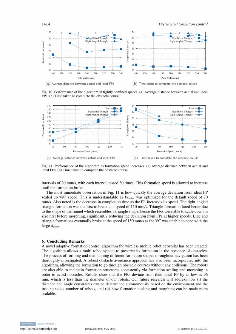
Fig. 10. Performance of the algorithm in tightly confined spaces. (a) Average distance between actual and idealFPs. (b) Time taken to complete the obstacle course.

80

100

120

140

160

180

200

220

240

260

280

70 80 90 100 110 120 130

Pos

itio

nal E

rror

(m

m)

Formation Speed (mm/s)




12

14

16

18

20

22

24

70 80 90 100 110 120 130

Com

plet

ion

Tim

e (s

)

Formation Speed (mm/s)




Fig. 11. Performance of the algorithm as formation speed increases. (a) Average distance between actual andideal FPs. (b) Time taken to complete the obstacle course.

intervals of 20 mm/s, with each interval tested 30 times. This formation speed is allowed to increaseuntil the formation broke.

The most immediate observation in Fig. 11 is how quickly the average deviation from ideal FPscaled up with speed. This is understandable as Vleader was optimized for the default speed of 70mm/s. Also noted is the decrease in completion time as the FL increases its speed. The right-angledtriangle formation was the first to break at a speed of 110 mm/s. Triangle formation fared better dueto the shape of the funnel which resembles a triangle shape, hence the FRs were able to scale down insize first before morphing, significantly reducing the deviation from FPs at higher speeds. Line andtriangle formations eventually broke at the speed of 150 mm/s as the VC was unable to cope with thelarge derror.

6. Concluding RemarksA novel adaptive formation control algorithm for wireless mobile robot networks has been created.The algorithm allows a multi robot system to preserve its formation in the presence of obstacles.The process of forming and maintaining different formation shapes throughout navigation has beenthoroughly investigated. A robust obstacle avoidance approach has also been incorporated into thealgorithm, allowing the formation to go through obstacle courses without any collisions. The robotsare also able to maintain formation structures consistently via formation scaling and morphing inorder to avoid obstacles. Results show that the FRs deviate from their ideal FP by as low as 96mm, which is less than the diameter of our robots. Our future research will address how (i) thedistance and angle constraints can be determined autonomously based on the environment and theinstantaneous number of robots, and (ii) how formation scaling and morphing can be made morescalable.




AcknowledgmentsThis research was supported in part by the Lise and Arnfinn Hejes Grant for Education and Research.

Supplementary materialTo view supplementary material for this article, please visit https://dl.dropboxusercontent.com/u/5574096/Distributed%20Formation%20Control%20of%20Networked%20Mobile%20Robots%20in%20Environments%20with%20Obstacles.wmv

References1. J. C. Barca and Y. A. Sekercioglu, “Swarm robotics reviewed,” Robotica (2012).2. J. Shao, G. Xie and L. Wang, “Leader following formation control of multiple mobile vehicles,” IET Control

Theory Appl. 1(2), 545–552 (2007).3. J. P. Desai, J. P. Ostrowski and V. Kumar, “Modeling and control of formations of nonholonomic mobile

robots,” IEEE Trans. Robot. Autom. 17(6), 905–908 (Dec. 2001).4. M. N. Soorki, H. A. Talebi and S. K. Y. Nikravesh, “A Robust Dynamic Leader-Follower Formation

Control with Active Obstacle Avoidance, IEEE International Conference on Systems, Man, and Cybernetics,Anchorage, Alaska, USA (2011) pp. 1932–1937.

5. M. N. Soorki, H. A. Talebi and S. K. Y. Nikravesh, “A Robust Leader-Obstacle Formation Control,” IEEEInternational Conference on Control Applications (2011) pp. 489–494.

6. S. Hou, C. Cheah and J. Slotine, “Dynamic Region Following Formation Control for a Swarm of Robots,”IEEE International Conference on Robotics and Automation (2009) pp. 1929–1934.

7. C. R. M. Kuppan, M. Singaperumal and T. Nagarajan, “Distributed Planning and Control of MultirobotFormations with Navigation and Obstacle Avoidance,” IEEE Recent Advances in Intelligent ComputationalSystems (2011) pp. 621–626.

8. A. S. Brandao, M. Sarcinelli-Filho, R. Carelli and T. F. Bastos-Filho, “Decentralized Control of Leader-Follower Formations of Mobile Robots with Obstacle Avoidance,” IEEE International Conference onMechatronics (2009) pp. 1–6.

9. J. C. Barca and Y. A. Sekercioglu, “Generating Formations with a Template based Multi-Robot System,”Australasian Conference on Robotics and Automation (2011).

10. Y. Liang and H.-H Lee, “Decentralized Formation Control and Obstacle Avoidance for Multiple Robotswith Nonholonomic Constraints,” American Control Conference (2006).

11. J. Wang, X.-B. Wu and Z.-L. Xu, “Decentralized Formation Control and Obstacles Avoidance basedon Potential Field Method,” International Conference on Machine Learning and Cybernetics (2006) pp.803–808.

12. J. P. Desai, J. P. Ostrowski and V. Kumar, “Formation Control and Obstacle Avoidance Algorithm ofMultiple Autonomous Underwater Vehicles (auvs) based on Potential Function and Behavior Rules,” IEEEInternational Conference on Automation and Logistics (2007) pp. 569–573.

13. N. D’Ademo, W. H. Li, D. Lui, Y. A. Sekercioglu and T. Drummond, “ebug - an Open Robotics Platformfor Teaching and Research, Australasian Conference on Robotics and Automation (2011).

14. J. C. Barca, Y. A. Sekercioglu and A. Ford, “Controlling Formations of Robots with Graph Theory,” 12thInternational Conference on Intelligent Autonomous Systems (2012) pp. 1–8.

15. P. Ogren and N. E. Leonard, “Obstacle Avoidance in Formation,” IEEE International Conference onRobotics and Automation, vol. 2 (2003) pp. 2492–2497.

16. A. K. Das, R. Fierro, V. Kumar, J. P. Ostrowski, J. Spletzer and C. J. Taylor, “A vision-based formationcontrol framework,” IEEE Trans. Robot. Autom. 18(5), 813–825 (2002).

17. B. Anderson, C. Yu, B. Fidan and J. Hendrickx, “Rigid graph control architectures for autonomousformations,” IEEE Control Syst. 28(6), 48–63 (2008).

18. Y.-C. Chen and Y.-T. Wang, “Obstacle Avoidance and Role Assignment Algorithms for Robot FormationControl,” IEEE/RSJ International Conference on Intelligent Robots and Systems (2007) pp. 4201–4206.

19. F. Yang, F. Liu, S. Liu and C. Zhong, “Hybrid Formation Control of Multiple Mobile Robots with ObstacleAvoidance,” 8th World Congress on Intelligent Control and Automation (2010) pp. 1039–1044.

20. Artoolkitplus. URL: http://studierstube.icg.tugraz.at/handheld ar/artoolkitplus.php.


Date post:	01-Apr-2020
Category:	Documents
Upload:	others
View:	40 times
Download:	1 times

Robotica · Robotica, Systems Control,”

Documents