69
Robots and Jobs: Evidence from US labor markets. Daron Acemoglu 1 Pascual Restrepo 2 1 MIT: [email protected] 2 Yale and Boston University [email protected] October 2016
| Date post: | 06-Apr-2018 |
| Category: |
Documents |
| Upload: | truongquynh |
| View: | 217 times |
| Download: | 2 times |
Robots and Jobs:
Evidence from US labor markets.
Daron Acemoglu 1 Pascual Restrepo 2
1MIT: [email protected]
2Yale and Boston University [email protected]
October 2016
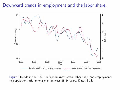
Downward trends in employment and the labor share.
.56
.58
.6.6
2.6
4.6
6Lab
or s
har
e
.8.8
5.9
.95
Em
plo
ymen
t ra
te
1955 1965 1975 1985 1995 2005 2015Year
Employment rate for prime-age men Labor share in nonfarm business
Figure: Trends in the U.S. nonfarm business sector labor share and employmentto population ratio among men between 25-54 years. Data: BLS.
Is automation responsible?
Mounting evidence that automation affects labor markets:
◮ Wage inequality and employment polarization (Autor, Levy &Murnane, 2003; Michaels, Natraj & Van Reenen, 2014).
◮ Firms that use new technologies demand different skills (Bartel,Ichniowski, & Shaw, 2007).
It is (or will soon be) feasible to automate many jobs.
◮ In the next 20 years, 50% of US jobs could be automated (Frey &Osborne, 2013; World Bank, 2016).
But does automation reduce employment and wages inequilibrium?
This paper
We estimate the employment and wage effects of industrialrobots on US labor markets.
◮ The International Federation of Robotics (IFR) defines them as:
“an automatically controlled, reprogrammable, and multipurpose[machine] that can be programmed in three or more axes for use inindustrial applications”
◮ Machines that do not need a human operator, and that can beprogrammed to perform several manual tasks such as welding,painting, assembling, sorting, handling materials, or packaging.
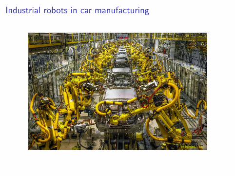
Industrial robots in car manufacturing
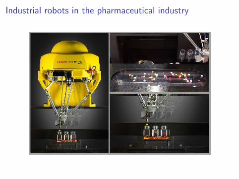
Industrial robots in the pharmaceutical industry
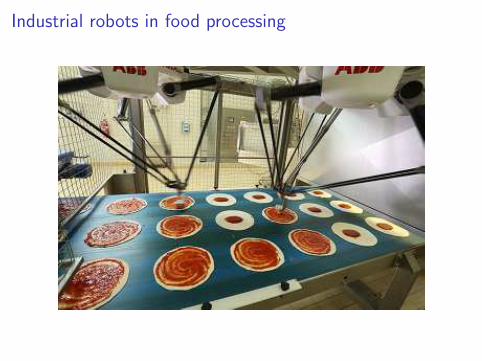
Industrial robots in food processing
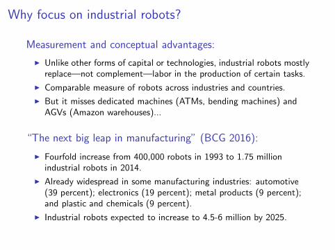
Why focus on industrial robots?
Measurement and conceptual advantages:
◮ Unlike other forms of capital or technologies, industrial robots mostlyreplace—not complement—labor in the production of certain tasks.
◮ Comparable measure of robots across industries and countries.
◮ But it misses dedicated machines (ATMs, bending machines) andAGVs (Amazon warehouses)...
“The next big leap in manufacturing” (BCG 2016):
◮ Fourfold increase from 400,000 robots in 1993 to 1.75 millionindustrial robots in 2014.
◮ Already widespread in some manufacturing industries: automotive(39 percent); electronics (19 percent); metal products (9 percent);and plastic and chemicals (9 percent).
◮ Industrial robots expected to increase to 4.5-6 million by 2025.
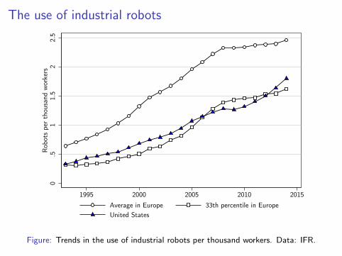
The use of industrial robots
0.5
11.
52
2.5
Rob
ots
per
thou
sand w
orke
rs
1995 2000 2005 2010 2015
Average in Europe 33th percentile in Europe
United States
Figure: Trends in the use of industrial robots per thousand workers. Data: IFR.
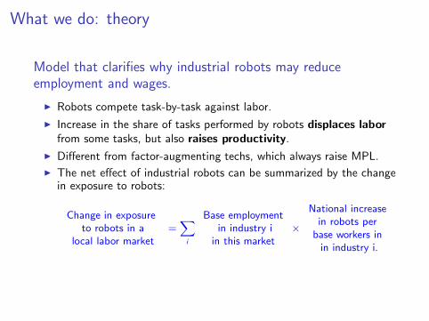
What we do: theory
Model that clarifies why industrial robots may reduceemployment and wages.
◮ Robots compete task-by-task against labor.
◮ Increase in the share of tasks performed by robots displaces labor
from some tasks, but also raises productivity.
◮ Different from factor-augmenting techs, which always raise MPL.
◮ The net effect of industrial robots can be summarized by the changein exposure to robots:
Change in exposureto robots in a
local labor market=∑
i
Base employmentin industry i
in this market×
National increasein robots perbase workers inin industry i.
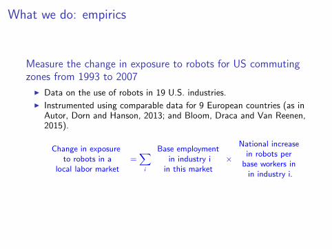
What we do: empirics
Measure the change in exposure to robots for US commutingzones from 1993 to 2007
◮ Data on the use of robots in 19 U.S. industries.
◮ Instrumented using comparable data for 9 European countries (as inAutor, Dorn and Hanson, 2013; and Bloom, Draca and Van Reenen,2015).
Change in exposureto robots in a
local labor market=∑
i
Base employmentin industry i
in this market×
National increasein robots perbase workers inin industry i.
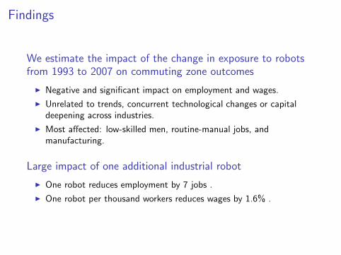
Findings
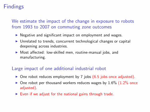
We estimate the impact of the change in exposure to robotsfrom 1993 to 2007 on commuting zone outcomes
◮ Negative and significant impact on employment and wages.
◮ Unrelated to trends, concurrent technological changes or capitaldeepening across industries.
◮ Most affected: low-skilled men, routine-manual jobs, andmanufacturing.
Large impact of one additional industrial robot
◮ One robot reduces employment by 7 jobs .
◮ One robot per thousand workers reduces wages by 1.6% .
Findings
We estimate the impact of the change in exposure to robotsfrom 1993 to 2007 on commuting zone outcomes
◮ Negative and significant impact on employment and wages.
◮ Unrelated to trends, concurrent technological changes or capitaldeepening across industries.
◮ Most affected: low-skilled men, routine-manual jobs, andmanufacturing.
Large impact of one additional industrial robot
◮ One robot reduces employment by 7 jobs (6.5 jobs once adjusted).
◮ One robot per thousand workers reduces wages by 1.6% (1.2% onceadjusted).
◮ Even if we adjust for the national gains through trade.
Aggregate implications
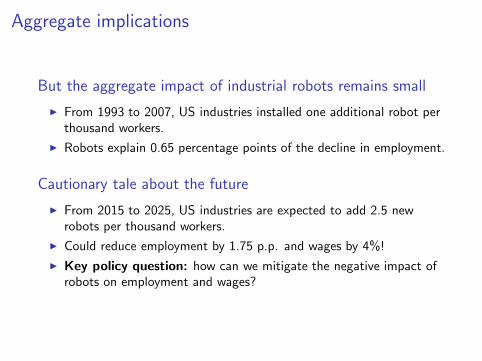
But the aggregate impact of industrial robots remains small
◮ From 1993 to 2007, US industries installed one additional robot perthousand workers.
◮ Robots explain 0.65 percentage points of the decline in employment.
Cautionary tale about the future
◮ From 2015 to 2025, US industries are expected to add 2.5 newrobots per thousand workers.
◮ Could reduce employment by 1.75 p.p. and wages by 4%!
◮ Key policy question: how can we mitigate the negative impact ofrobots on employment and wages?
Related literature
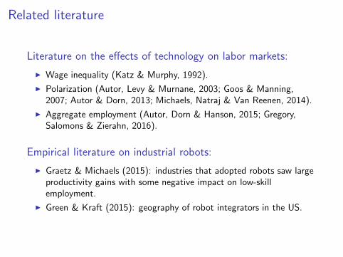
Literature on the effects of technology on labor markets:
◮ Wage inequality (Katz & Murphy, 1992).
◮ Polarization (Autor, Levy & Murnane, 2003; Goos & Manning,2007; Autor & Dorn, 2013; Michaels, Natraj & Van Reenen, 2014).
◮ Aggregate employment (Autor, Dorn & Hanson, 2015; Gregory,Salomons & Zierahn, 2016).
Empirical literature on industrial robots:
◮ Graetz & Michaels (2015): industries that adopted robots saw largeproductivity gains with some negative impact on low-skillemployment.
◮ Green & Kraft (2015): geography of robot integrators in the US.
Outline for the rest of the talk
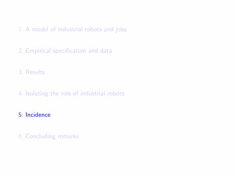
1. A model of industrial robots and jobs
2. Empirical specification and data
3. Results
4. Isolating the role of industrial robots
5. Incidence
6. Concluding remarks
1. A model of industrial robots and jobs
2. Empirical specification and data
3. Results
4. Isolating the role of industrial robots
5. Incidence
6. Concluding remarks
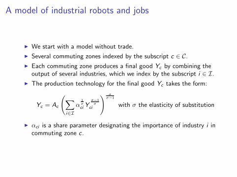
A model of industrial robots and jobs
◮ We start with a model without trade.
◮ Several commuting zones indexed by the subscript c ∈ C.
◮ Each commuting zone produces a final good Yc by combining theoutput of several industries, which we index by the subscript i ∈ I.
◮ The production technology for the final good Yc takes the form:
Yc = Ac
(∑
i∈I
α1σ
ciY
σ−1σ
ci
) σ
σ−1
with σ the elasticity of substitution
◮ αci is a share parameter designating the importance of industry i incommuting zone c .
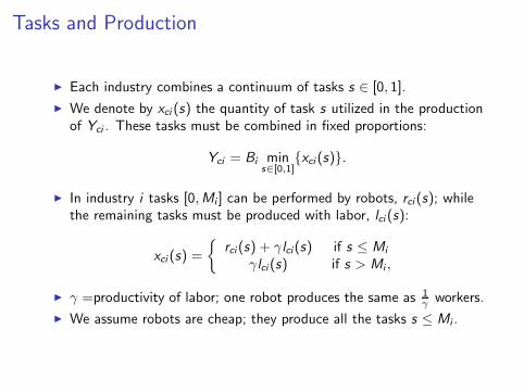
Tasks and Production
◮ Each industry combines a continuum of tasks s ∈ [0, 1].
◮ We denote by xci (s) the quantity of task s utilized in the productionof Yci . These tasks must be combined in fixed proportions:
Yci = Bi mins∈[0,1]
{xci (s)}.
◮ In industry i tasks [0,Mi ] can be performed by robots, rci (s); whilethe remaining tasks must be produced with labor, lci (s):
xci (s) =
{rci (s) + γlci(s) if s ≤ Mi
γlci (s) if s > Mi ,
◮ γ =productivity of labor; one robot produces the same as 1γworkers.
◮ We assume robots are cheap; they produce all the tasks s ≤ Mi .
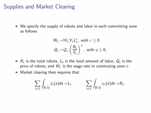
Supplies and Market Clearing
◮ We specify the supply of robots and labor in each committing zoneas follows
Wc =WcYcLε
c, with ε ≥ 0.
Qc =Qc
(Rc
Yc
)η
, with η ≥ 0,
◮ Rc is the total robots, Lc is the total amount of labor, Qc is theprice of robots, and Wc is the wage rate in commuting zone c .
◮ Market clearing then requires that
∑
i∈I
∫
[0,1]
lci (s)ds =Lc∑
i∈I
∫
[0,1]
rci (s)ds =Rc .
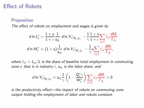
Effect of Robots
PropositionThe effect of robots on employment and wages is given by
d ln L∗c=
1 + η
1 + ε
1
scLd lnYc |Rc ,Lc
−1
γ
1 + η
1 + ε
∑
i∈I
ℓcidMi
ΓiL
d lnW ∗c= (1 + η)
1
scLd lnYc |Rc ,Lc
−1
γη∑
i∈I
ℓcidMi
ΓiL,
where ℓci = Lci/L is the share of baseline total employment in commutingzone c that is in industry i , scL is the labor share, and
d lnYc |Rc ,Lc= scL
1
γ
(1−
Q∗cγ
W ∗c
)∑
i∈I
ℓcidMi
ΓiL> 0
is the productivity effect—the impact of robots on commuting zoneoutput holding the employment of labor and robots constant.
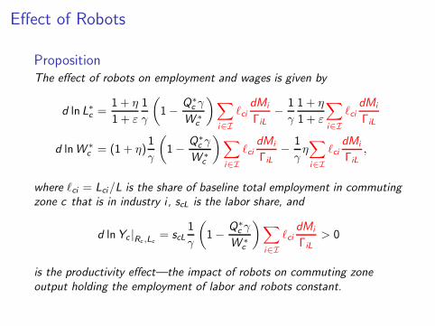
Effect of Robots
PropositionThe effect of robots on employment and wages is given by
d ln L∗c =1 + η
1 + ε
1
γ
(1−
Q∗cγ
W ∗c
)∑
i∈I
ℓcidMi
ΓiL−
1
γ
1 + η
1 + ε
∑
i∈I
ℓcidMi
ΓiL
d lnW ∗c= (1 + η)
1
γ
(1−
Q∗cγ
W ∗c
)∑
i∈I
ℓcidMi
ΓiL−
1
γη∑
i∈I
ℓcidMi
ΓiL,
where ℓci = Lci/L is the share of baseline total employment in commutingzone c that is in industry i , scL is the labor share, and
d lnYc |Rc ,Lc= scL
1
γ
(1−
Q∗cγ
W ∗c
)∑
i∈I
ℓcidMi
ΓiL> 0
is the productivity effect—the impact of robots on commuting zoneoutput holding the employment of labor and robots constant.
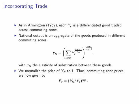
Incorporating Trade
◮ As in Armington (1969), each Yc is a differentiated good tradedacross commuting zones.
◮ National output is an aggregate of the goods produced in differentcommuting zones:
YN =
(∑
c∈C
YσN−1
σN
c
) σN
σN−1
,
with σN the elasticity of substitution between these goods.
◮ We normalize the price of YN to 1. Thus, commuting zone pricesare now given by
Pc = (YN/Yc)1
σN .
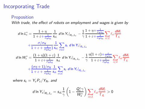
Incorporating Trade
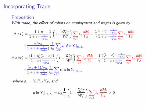
PropositionWith trade, the effect of robots on employment and wages is given by
d ln L∗c =
1 + η
1 + ε+ 1σN scL
1
scLd lnYc |Rc ,Lc
−1
γ
1 + η+ 1σN scL
1 + ε+ 1σN scL
∑
i∈I
ℓcidMi
ΓiL
+σ/σN
1 + ε+ 1σN scL
)
1
scL
∑
c∈C
sc d lnYc |Rc ,Lc
d lnW ∗c =
(1 + η)(1 + ε)
1 + ε+ 1σN scL
1
scLd lnYc |Rc ,Lc
−1
γ
η(1 + ε)+ ε
σN scL
1 + ε+ 1σN scL
∑
i∈I
ℓcidMi
ΓiL
+(ση + 1)/σN
1 + ε+ 1σN scL
1
scL
∑
c∈C
sc d lnYc |Rc ,Lc
where sc = YcPc/YN , and
d lnYc |Rc ,Lc= scL
1
γ
(1−
Q∗c γ
W ∗c
)∑
i∈I
ℓcidMi
ΓiL> 0
Incorporating Trade
PropositionWith trade, the effect of robots on employment and wages is given by
d lnL∗c =
1 + η
1 + ε+ 1σN scL
1
γ
(1−
Q∗c γ
W ∗c
)∑
i∈I
ℓcidMi
ΓiL
−1
γ
1 + η+ 1σN scL
1 + ε+ 1σN scL
∑
i∈I
ℓcidMi
ΓiL
+σ/σN
1 + ε+ 1σN scL
)
1
scL
∑
c∈C
sc d lnYc |Rc ,Lc
d lnW ∗c =
(1 + η)(1 + ε)
1 + ε+ 1σN scL
1
γ
(1−
Q∗c γ
W ∗c
)∑
i∈I
ℓcidMi
ΓiL
−1
γ
η(1 + ε)+ ε
σN scL
1 + ε+ 1σN scL
∑
i∈I
ℓcidMi
ΓiL
+(ση + 1)/σN
1 + ε+ 1σN scL
1
scL
∑
c∈C
sc d lnYc |Rc ,Lc
where sc = YcPc/YN , and
d lnYc |Rc ,Lc= scL
1
γ
(1−
Q∗c γ
W ∗c
)∑
i∈I
ℓcidMi
ΓiL> 0
1. A model of industrial robots and jobs
2. Empirical specification and data
3. Results
4. Isolating the role of industrial robots
5. Incidence
6. Concluding remarks
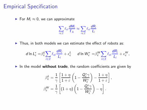
Empirical Specification
◮ For Mi ≈ 0, we can approximate
∑
i∈I
ℓcidMi
ΓiL
≈∑
i∈I
ℓcidRi
Li
◮ Thus, in both models we can estimate the effect of robots as:
d ln L∗c =βL
c
∑
i∈I
ℓcidRi
Li+ ǫLc d lnW ∗
c =βW
c
∑
i∈I
ℓcidRi
Li+ ǫWc ,
◮ In the model without trade, the random coefficients are given by
βL
c =1
γ
[1 + η
1 + ε
(1−
Q∗cγ
W ∗c
)−
1 + η
1 + ε
],
βW
c=
1
γ
[(1 + η)
(1−
Q∗c γ
W ∗c
)− η
].
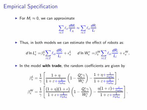
Empirical Specification
◮ For Mi ≈ 0, we can approximate
∑
i∈I
ℓcidMi
ΓiL
≈∑
i∈I
ℓcidRi
Li
◮ Thus, in both models we can estimate the effect of robots as:
d ln L∗c =βL
c
∑
i∈I
ℓcidRi
Li+ ǫLc d lnW ∗
c =βW
c
∑
i∈I
ℓcidRi
Li+ ǫWc ,
◮ In the model with trade, the random coefficients are given by
βL
c =1
γ
[1 + η
1 + ε+ 1σN scL
(1−
Q∗cγ
W ∗c
)−
1 + η+ 1σN scL
1 + ε+ 1σN scL
],
βW
c =1
γ
[(1 + η)(1 + ǫ)
1 + ǫ+ 1σN scL
(1−
Q∗c γ
W ∗c
)−
η(1 + ε)+ ε
σN scL
1 + ε+ 1σN scL
].
Data
Data for 722 US commuting zones:
◮ Commuting zones≈local labor markets.
◮ Census (or ACS) data for 722 commuting zones: employment,wages, and demographics for 1970, 1990, 2007.
◮ CBP data aggregated to the commuting zone level. Yearly from1988-2014.
◮ Complemented with IRS data on income and nonwage income.
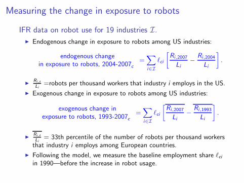
Measuring the change in exposure to robots
IFR data on robot use for 19 industries I.
◮ Endogenous change in exposure to robots among US industries:
endogenous changein exposure to robots, 2004-2007c
=∑
i∈I
ℓci
[Ri ,2007
Li−
Ri ,2004
Li
].
◮Ri,t
Li
=robots per thousand workers that industry i employs in the US.
◮ Exogenous change in exposure to robots among US industries:
exogenous change inexposure to robots, 1993-2007c
=∑
i∈I
ℓci
[Ri ,2007
Li−
Ri ,1993
Li
].
◮Ri,t
Li
= 33th percentile of the number of robots per thousand workersthat industry i employs among European countries.
◮ Following the model, we measure the baseline employment share ℓciin 1990—before the increase in robot usage.
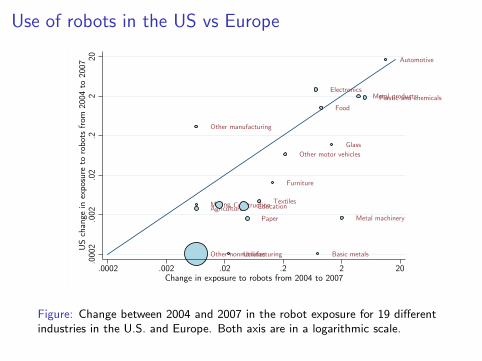
Use of robots in the US vs Europe
Agriculture
Automotive
ConstructionEducation
Electronics
Food
Furniture
Glass
Other manufacturing
Basic metals
Metal machinery
Metal products
Mining
Other nonmanufacturing
Paper
Plastic and chemicals
Textiles
Utilities
Other motor vehicles
.000
2.0
02.0
2.2
220
US c
han
ge in e
xpos
ure
to
robot
s from
200
4 to
200
7
.0002 .002 .02 .2 2 20Change in exposure to robots from 2004 to 2007
Figure: Change between 2004 and 2007 in the robot exposure for 19 differentindustries in the U.S. and Europe. Both axis are in a logarithmic scale.
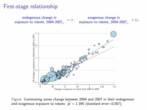
First-stage relationship
endogenous change inexposure to robots, 2004-2007
c
= π ·exogenous change in
exposure to robots, 2004-2007c
+ νc .
0.5
11.
52
US C
han
ge in e
xpos
ure
to
robot
s from
200
4 to
200
7
0 .25 .5 .75 1 1.25 1.5Change in exposure to robots from 2004 to 2007
Figure: Commuting zones change between 2004 and 2007 in their endogenousand exogenous exposure to robots. pi = 1.395 (standard error=0.057).
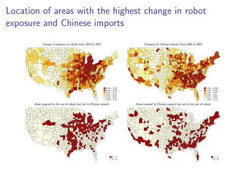
Location of areas with the highest change in robot
exposure and Chinese imports
0.93 − 2.880.70 − 0.930.55 − 0.700.41 − 0.550.28 − 0.410.09 − 0.28
Change in exposure to robots from 1993 to 2007
2.56 − 10.361.57 − 2.561.05 − 1.570.64 − 1.050.21 − 0.64-0.03 − 0.21
Exposure to Chinese imports from 1990 to 2007
0 − 10 − 0
Areas exposed to the use of robots but not to Chinese imports
0 − 10 − 0
Areas exposed to Chinese imports but not to the use of robots
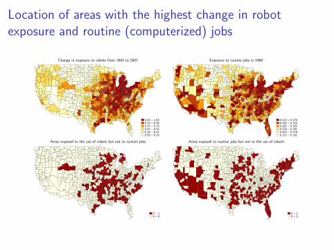
Location of areas with the highest change in robot
exposure and routine (computerized) jobs
0.93 − 2.880.70 − 0.930.55 − 0.700.41 − 0.550.28 − 0.410.09 − 0.28
Change in exposure to robots from 1993 to 2007
0.323 − 0.3780.305 − 0.3230.291 − 0.3050.279 − 0.2910.262 − 0.2790.222 − 0.262
Exposure to routine jobs in 1990
0 − 10 − 0
Areas exposed to the use of robots but not to routine jobs
0 − 10 − 0
Areas exposed to routine jobs but not to the use of robots
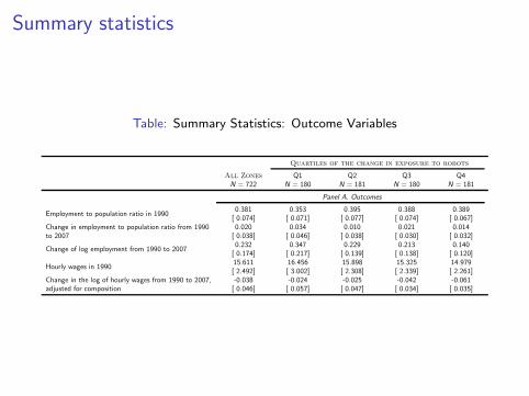
Summary statistics
Table: Summary Statistics: Outcome Variables
Quartiles of the change in exposure to robots
All Zones Q1 Q2 Q3 Q4N = 722 N = 180 N = 181 N = 180 N = 181
Panel A. Outcomes
Employment to population ratio in 19900.381 0.353 0.395 0.388 0.389[ 0.074] [ 0.071] [ 0.077] [ 0.074] [ 0.067]
Change in employment to population ratio from 1990to 2007
0.020 0.034 0.010 0.021 0.014[ 0.038] [ 0.046] [ 0.038] [ 0.030] [ 0.032]
Change of log employment from 1990 to 20070.232 0.347 0.229 0.213 0.140[ 0.174] [ 0.217] [ 0.139] [ 0.138] [ 0.120]
Hourly wages in 199015.611 16.456 15.898 15.325 14.979[ 2.492] [ 3.002] [ 2.308] [ 2.339] [ 2.261]
Change in the log of hourly wages from 1990 to 2007,adjusted for composition
-0.038 -0.024 -0.025 -0.042 -0.061[ 0.046] [ 0.057] [ 0.047] [ 0.034] [ 0.035]
1. A model of industrial robots and jobs
2. Empirical specification and data
3. Results
4. Isolating the role of industrial robots
5. Incidence
6. Concluding remarks
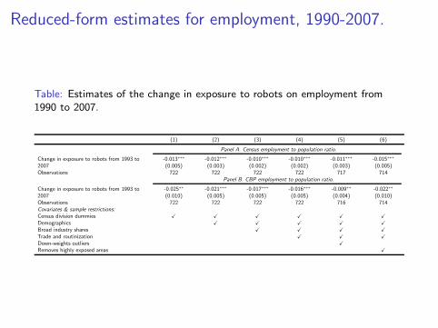
Reduced-form estimates for employment, 1990-2007.
Table: Estimates of the change in exposure to robots on employment from1990 to 2007.
(1) (2) (3) (4) (5) (6)
Panel A. Census employment to population ratio.
Change in exposure to robots from 1993 to2007
-0.013∗∗∗ -0.012∗∗∗ -0.010∗∗∗ -0.010∗∗∗ -0.011∗∗∗ -0.015∗∗∗
(0.005) (0.003) (0.002) (0.002) (0.003) (0.005)Observations 722 722 722 722 717 714
Panel B. CBP employment to population ratio.
Change in exposure to robots from 1993 to2007
-0.025∗∗ -0.021∗∗∗ -0.017∗∗∗ -0.016∗∗∗ -0.009∗∗ -0.022∗∗
(0.010) (0.005) (0.005) (0.005) (0.004) (0.010)Observations 722 722 722 722 716 714Covariates & sample restrictions:Census division dummies X X X X X X
Demographics X X X X X
Broad industry shares X X X X
Trade and routinization X X X
Down-weights outliers X
Removes highly exposed areas X
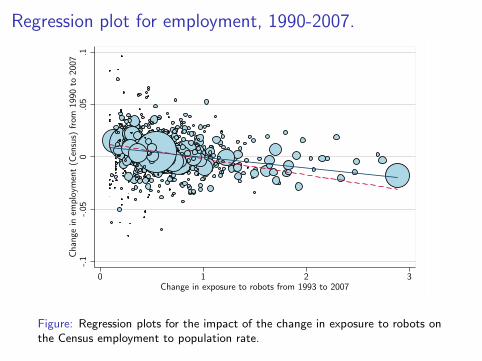
Regression plot for employment, 1990-2007.
-.1
-.05
0.0
5.1
Chan
ge in e
mplo
ymen
t (C
ensu
s) fro
m 1
990
to 2
007
0 1 2 3Change in exposure to robots from 1993 to 2007
Figure: Regression plots for the impact of the change in exposure to robots onthe Census employment to population rate.
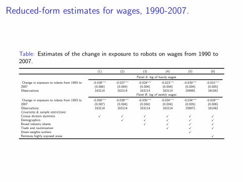
Reduced-form estimates for wages, 1990-2007.
Table: Estimates of the change in exposure to robots on wages from 1990 to2007.
(1) (2) (3) (4) (5) (6)
Panel A. log of hourly wages
Change in exposure to robots from 1993 to2007
-0.038∗∗∗ -0.027∗∗∗ -0.024∗∗∗ -0.023∗∗∗ -0.030∗∗∗ -0.031∗∗∗
(0.006) (0.004) (0.004) (0.004) (0.004) (0.005)Observations 163114 163114 163114 163114 159991 161042
Panel B. log of weekly wages
Change in exposure to robots from 1993 to2007
-0.050∗∗∗ -0.039∗∗∗ -0.035∗∗∗ -0.034∗∗∗ -0.034∗∗∗ -0.039∗∗∗
(0.007) (0.004) (0.004) (0.004) (0.005) (0.006)Observations 163114 163114 163114 163114 159671 161042Covariates & sample restrictions:Census division dummies X X X X X X
Demographics X X X X X
Broad industry shares X X X X
Trade and routinization X X X
Down-weights outliers X
Removes highly exposed areas X
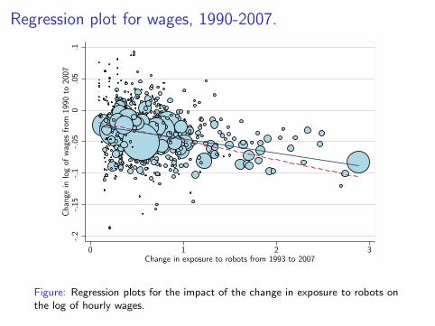
Regression plot for wages, 1990-2007.
-.2
-.15
-.1
-.05
0.0
5.1
Chan
ge in log
of w
ages
fro
m 1
990
to 2
007
0 1 2 3Change in exposure to robots from 1993 to 2007
Figure: Regression plots for the impact of the change in exposure to robots onthe log of hourly wages.
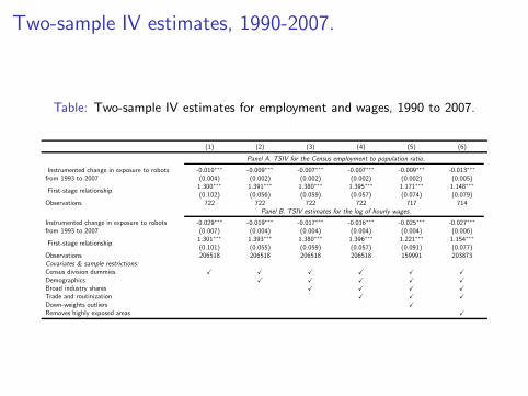
Two-sample IV estimates, 1990-2007.
Table: Two-sample IV estimates for employment and wages, 1990 to 2007.
(1) (2) (3) (4) (5) (6)
Panel A. TSIV for the Census employment to population ratio.
Instrumented change in exposure to robotsfrom 1993 to 2007
-0.010∗∗∗ -0.009∗∗∗ -0.007∗∗∗ -0.007∗∗∗ -0.009∗∗∗ -0.013∗∗∗
(0.004) (0.002) (0.002) (0.002) (0.002) (0.005)
First-stage relationship1.300∗∗∗ 1.391∗∗∗ 1.380∗∗∗ 1.395∗∗∗ 1.171∗∗∗ 1.148∗∗∗
(0.102) (0.056) (0.059) (0.057) (0.074) (0.079)Observations 722 722 722 722 717 714
Panel B. TSIV estimates for the log of hourly wages.
Instrumented change in exposure to robotsfrom 1993 to 2007
-0.029∗∗∗ -0.019∗∗∗ -0.017∗∗∗ -0.016∗∗∗ -0.025∗∗∗ -0.027∗∗∗
(0.007) (0.004) (0.004) (0.004) (0.004) (0.006)
First-stage relationship1.301∗∗∗ 1.393∗∗∗ 1.380∗∗∗ 1.396∗∗∗ 1.221∗∗∗ 1.154∗∗∗
(0.101) (0.055) (0.059) (0.057) (0.091) (0.077)Observations 206518 206518 206518 206518 159991 203873Covariates & sample restrictions:Census division dummies X X X X X X
Demographics X X X X X
Broad industry shares X X X X
Trade and routinization X X X
Down-weights outliers X
Removes highly exposed areas X
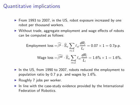
Quantitative implications
◮ From 1993 to 2007, in the US, robot exposure increased by onerobot per thousand workers.
◮ Without trade, aggregate employment and wage effects of robotscan be computed as follows:
Employment loss =βL · Ec
∑
i∈I
ℓcidRi
Li= 0.07× 1 = 0.7p.p.
Wage loss =βW · Ec
∑
i∈I
ℓcidRi
Li= 1.6%× 1 = 1.6%.
◮ In the US, from 1990 to 2007, robots reduced the employment topopulation ratio by 0.7 p.p. and wages by 1.6%.
◮ Roughly 7 jobs per worker.
◮ In line with the case-study evidence provided by the InternationalFederation of Robotics.
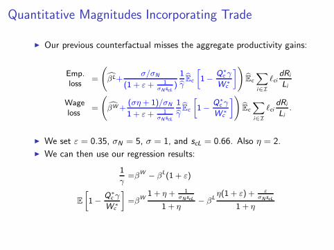
Quantitative Magnitudes Incorporating Trade
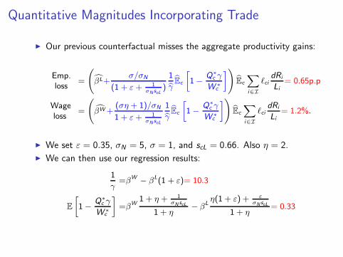
◮ Our previous counterfactual misses the aggregate productivity gains:
Emp.loss
=
(βL+
σ/σN
(1 + ε+ 1σN scL
)
1
γEc
[1−
Q∗c γ
W ∗c
])Ec
∑
i∈I
ℓcidRi
Li
Wageloss
=
(βW+
(ση + 1)/σN
1 + ε+ 1σN scL
1
γEc
[1−
Q∗c γ
W ∗c
])Ec
∑
i∈I
ℓcidRi
Li
.
◮ We set ε = 0.35, σN = 5, σ = 1, and scL = 0.66. Also η = 2.
◮ We can then use our regression results:
1
γ=βW − βL(1 + ε)
E
[1−
Q∗c γ
W ∗c
]=βW
1 + η + 1σN scL
1 + η− βL
η(1 + ε) + ε
σN scL
1 + η
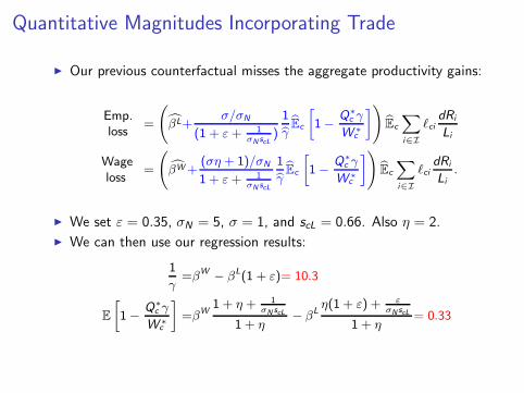
Quantitative Magnitudes Incorporating Trade
◮ Our previous counterfactual misses the aggregate productivity gains:
Emp.loss
=
(βL+
σ/σN
(1 + ε+ 1σN scL
)
1
γEc
[1−
Q∗c γ
W ∗c
])Ec
∑
i∈I
ℓcidRi
Li
Wageloss
=
(βW+
(ση + 1)/σN
1 + ε+ 1σN scL
1
γEc
[1−
Q∗c γ
W ∗c
])Ec
∑
i∈I
ℓcidRi
Li
.
◮ We set ε = 0.35, σN = 5, σ = 1, and scL = 0.66. Also η = 2.
◮ We can then use our regression results:
1
γ=βW − βL(1 + ε)= 10.3
E
[1−
Q∗c γ
W ∗c
]=βW
1 + η + 1σN scL
1 + η− βL
η(1 + ε) + ε
σN scL
1 + η= 0.33
Quantitative Magnitudes Incorporating Trade
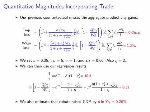
◮ Our previous counterfactual misses the aggregate productivity gains:
Emp.loss
=
(βL+
σ/σN
(1 + ε+ 1σN scL
)
1
γEc
[1−
Q∗c γ
W ∗c
])Ec
∑
i∈I
ℓcidRi
Li
= 0.65p.p
Wageloss
=
(βW+
(ση + 1)/σN
1 + ε+ 1σN scL
1
γEc
[1−
Q∗c γ
W ∗c
])Ec
∑
i∈I
ℓcidRi
Li
= 1.2%.
◮ We set ε = 0.35, σN = 5, σ = 1, and scL = 0.66. Also η = 2.
◮ We can then use our regression results:
1
γ=βW − βL(1 + ε)= 10.3
E
[1−
Q∗c γ
W ∗c
]=βW
1 + η + 1σN scL
1 + η− βL
η(1 + ε) + ε
σN scL
1 + η= 0.33
Quantitative Magnitudes Incorporating Trade
◮ Our previous counterfactual misses the aggregate productivity gains:
Emp.loss
=
(βL+
σ/σN
(1 + ε+ 1σN scL
)
1
γEc
[1−
Q∗c γ
W ∗c
])Ec
∑
i∈I
ℓcidRi
Li
= 0.65p.p
Wageloss
=
(βW+
(ση + 1)/σN
1 + ε+ 1σN scL
1
γEc
[1−
Q∗c γ
W ∗c
])Ec
∑
i∈I
ℓcidRi
Li
= 1.2%.
◮ We set ε = 0.35, σN = 5, σ = 1, and scL = 0.66. Also η = 2.
◮ We can then use our regression results:
1
γ=βW − βL(1 + ε)= 10.3
E
[1−
Q∗c γ
W ∗c
]=βW
1 + η + 1σN scL
1 + η− βL
η(1 + ε) + ε
σN scL
1 + η= 0.33
◮ We also estimate that robots raised GDP by d lnYN = 0.26%
1. A model of industrial robots and jobs
2. Empirical specification and data
3. Results
4. Isolating the role of industrial robots
5. Incidence
6. Concluding remarks
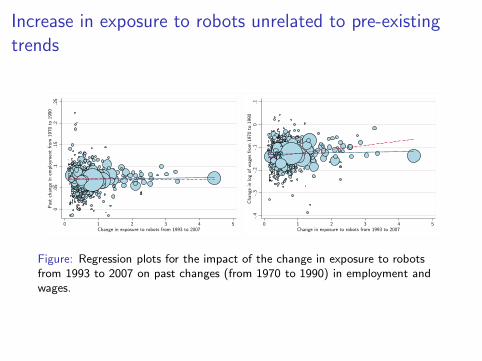
Increase in exposure to robots unrelated to pre-existing
trends0
.05
.1.1
5.2
.25
Pas
t ch
ange
in e
mplo
ymen
t from
197
0 to
199
0
0 1 2 3 4 5Change in exposure to robots from 1993 to 2007
-.4
-.3
-.2
-.1
0.1
Chan
ge in log
of w
ages
fro
m 1
970
to 1
990
0 1 2 3 4 5Change in exposure to robots from 1993 to 2007
Figure: Regression plots for the impact of the change in exposure to robotsfrom 1993 to 2007 on past changes (from 1970 to 1990) in employment andwages.
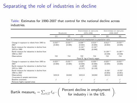
Separating the role of industries in decline
Table: Estimates for 1990-2007 that control for the national decline acrossindustries.
Industries in decline Industries in decline
Baseline 1970-1990 1990-2007
(1) (2) (3) (4) (5) (6)
Panel A. Census private employment to population ratio.
Change in exposure to robots from 1993 to2007
-0.010∗∗∗ -0.015∗∗∗ -0.009∗∗∗ -0.014∗∗∗ -0.012∗∗∗ -0.018∗∗∗
(0.002) (0.005) (0.002) (0.005) (0.002) (0.005)Bartik measure for industries in decline from1970 to 1990
-0.116∗∗ -0.110∗∗
(0.048) (0.048)Bartik measure for industries in decline from1990 to 2007
-0.139∗∗∗ -0.138∗∗∗
(0.039) (0.038)Observations 722 714 722 714 722 714
Panel B. log of hourly wages.
Change in exposure to robots from 1993 to2007
-0.023∗∗∗ -0.031∗∗∗ -0.022∗∗∗ -0.030∗∗∗ -0.025∗∗∗ -0.033∗∗∗
(0.004) (0.005) (0.004) (0.006) (0.004) (0.005)Bartik measure for industries in decline from1970 to 1990
-0.097 -0.083(0.117) (0.118)
Bartik measure for industries in decline from1990 to 2007
-0.155∗ -0.153∗
(0.083) (0.081)Observations 163114 161042 163114 161042 163114 161042Covariates & sample restrictions:Baseline covariates X X X X X X
Removes highly exposed areas X X X
Bartik measurec =∑
i∈Iℓci ·
(Percent decline in employment
for industry i in the US.
).
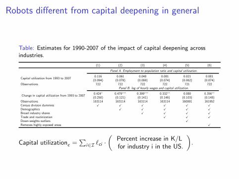
Robots different from capital deepening in general
Table: Estimates for 1990-2007 of the impact of capital deepening acrossindustries.
(1) (2) (3) (4) (5) (6)
Panel A. Employment to population ratio and capital utilization.
Capital utilization from 1993 to 20070.116 0.061 0.048 0.081 0.021 0.081(0.094) (0.078) (0.069) (0.074) (0.062) (0.074)
Observations 722 722 722 722 721 722Panel B. log of hourly wages and capital utilization.
Change in capital utilization from 1993 to 20070.424∗ 0.479∗∗∗ 0.399∗∗∗ 0.332∗∗ 0.080 0.356∗∗
(0.250) (0.121) (0.141) (0.146) (0.103) (0.148)Observations 163114 163114 163114 163114 160001 161952Census division dummies X X X X X X
Demographics X X X X X
Broad industry shares X X X X
Trade and routinization X X X
Down-weights outliers X
Removes highly exposed areas X
Capital utilizationc=∑
i∈Iℓci ·
(Percent increase in K/Lfor industry i in the US.
).
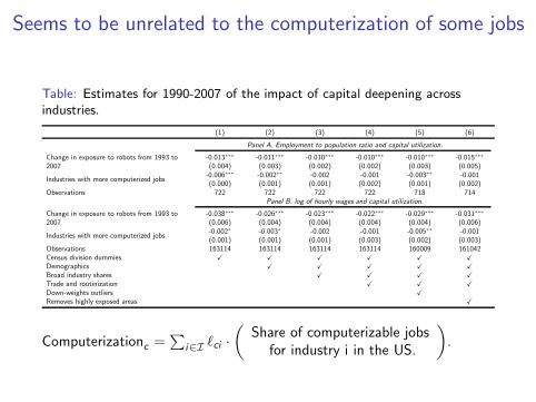
Seems to be unrelated to the computerization of some jobs
Table: Estimates for 1990-2007 of the impact of capital deepening acrossindustries.
(1) (2) (3) (4) (5) (6)
Panel A. Employment to population ratio and capital utilization.
Change in exposure to robots from 1993 to2007
-0.013∗∗∗ -0.011∗∗∗ -0.010∗∗∗ -0.010∗∗∗ -0.010∗∗∗ -0.015∗∗∗
(0.004) (0.003) (0.002) (0.002) (0.003) (0.005)
Industries with more computerized jobs-0.006∗∗∗ -0.002∗∗ -0.002 -0.001 -0.003∗∗ -0.001(0.000) (0.001) (0.001) (0.002) (0.001) (0.002)
Observations 722 722 722 722 718 714Panel B. log of hourly wages and capital utilization.
Change in exposure to robots from 1993 to2007
-0.038∗∗∗ -0.026∗∗∗ -0.023∗∗∗ -0.022∗∗∗ -0.029∗∗∗ -0.031∗∗∗
(0.006) (0.004) (0.004) (0.004) (0.004) (0.006)
Industries with more computerized jobs-0.002∗ -0.003∗ -0.002 -0.001 -0.005∗∗ -0.001(0.001) (0.001) (0.001) (0.003) (0.002) (0.003)
Observations 163114 163114 163114 163114 160009 161042Census division dummies X X X X X X
Demographics X X X X X
Broad industry shares X X X X
Trade and routinization X X X
Down-weights outliers X
Removes highly exposed areas X
Computerizationc =∑
i∈Iℓci ·
(Share of computerizable jobs
for industry i in the US.
).
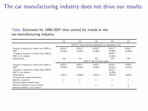
The car manufacturing industry does not drive our results
Table: Estimates for 1990-2007 that control for trends in thecar-manufacturing industry.
(1) (2) (3) (4) (5)
Panel A. Census private employment to population ratio.
Change in exposure to robots from 1993 to2007
-0.010∗∗∗ -0.015∗∗∗ -0.018∗∗∗ -0.021∗∗∗ -0.020∗∗∗
(0.002) (0.005) (0.005) (0.004) (0.005)Change in exposure to robots from 1993 to2007 in car industry
-0.009∗∗∗
(0.002)Observations 722 714 722 722 722
Panel B. log of hourly wages.
Change in exposure to robots from 1993 to2007
-0.023∗∗∗ -0.031∗∗∗ -0.024∗∗ -0.031∗∗∗ -0.026∗∗
(0.004) (0.005) (0.012) (0.011) (0.011)Change in exposure to robots from 1993 to2007 in car industry
-0.021∗∗∗
(0.004)Observations 163114 161042 163114 163114 162551Covariates & sample restrictions:Baseline covariates X X X X X
Removes highly exposed areas X
Removes exposure to auto industry X X X
Removes people in auto industry X
1. A model of industrial robots and jobs
2. Empirical specification and data
3. Results
4. Isolating the role of industrial robots
5. Incidence
6. Concluding remarks
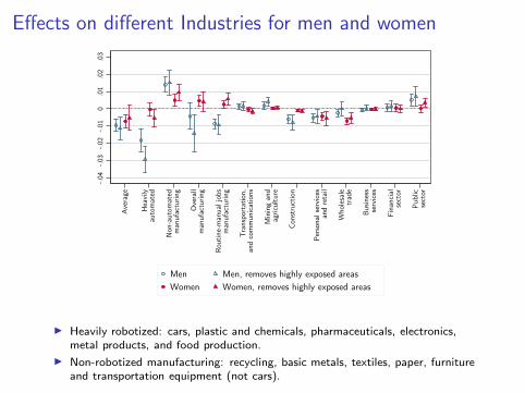
Effects on different Industries for men and women
-.04
-.03
-.02
-.01
0.0
1.0
2.0
3
Ave
rage
Hea
vily
auto
mat
ed
Non
-auto
mat
edm
anufa
cturing
Ove
rall
man
ufa
cturing
Rou
tine-
man
ual
job
sm
anufa
cturing
Tra
nsp
orta
tion
, a
nd c
omm
unic
atio
ns
Min
ing
and
agricu
lture
Con
stru
ctio
n
Per
sonal
ser
vice
san
d r
etai
l
Whol
esal
etr
ade
Busines
sse
rvic
es
Fin
anci
alse
ctor
Public
sect
or
Men Men, removes highly exposed areas
Women Women, removes highly exposed areas
◮ Heavily robotized: cars, plastic and chemicals, pharmaceuticals, electronics,metal products, and food production.
◮ Non-robotized manufacturing: recycling, basic metals, textiles, paper, furnitureand transportation equipment (not cars).
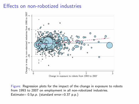
Effects on non-robotized industries
-.1
-.05
0.0
5.1
Chan
ge in e
mp. in
non
-rob
otiz
ed indust
ries
fro
m 1
990
to 2
007
0 1 2 3Change in exposure to robots from 1993 to 2007
Figure: Regression plots for the impact of the change in exposure to robotsfrom 1993 to 2007 on employment in all non-robotized industries.Estimate= 0.5p.p. (standard error=0.37 p.p.)
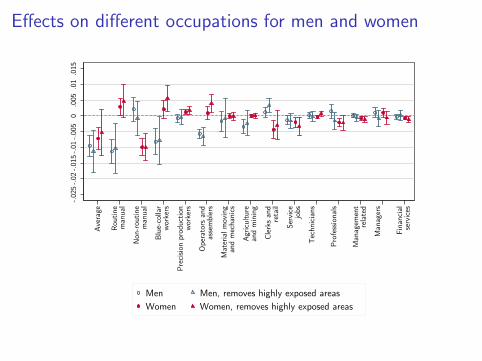
Effects on different occupations for men and women
-.02
5-.02
-.01
5-.01
-.00
50
.005
.01
.015
Ave
rage
Rou
tine
man
ual
Non
-rou
tine
man
ual
Blu
e-co
llar
wor
kers
Pre
cision
pro
duct
ion
wor
kers
Oper
ator
s an
das
sem
ble
rs
Mat
eria
l m
ovin
gan
d m
echan
ics
Agr
iculture
and m
inin
g
Cle
rks
and
reta
il
Ser
vice
jobs
Tec
hnic
ians
Pro
fess
ional
s
Man
agem
ent
rela
ted
Man
ager
s
Fin
anci
alse
rvic
es
Men Men, removes highly exposed areas
Women Women, removes highly exposed areas

Effects on workers with different skills
-.03
-.02
-.01
0.0
1.0
2
Ave
rage
Les
s th
anhig
hsc
hoo
l
Com
ple
ted
hig
hsc
hoo
l
Som
eco
llege
Com
ple
ted
colle
ge
Mas
ters
deg
ree
Men Men, removes highly exposed areas
Women Women, removes highly exposed areas
1. A model of industrial robots and jobs
2. Empirical specification and data
3. Results
4. Isolating the role of industrial robots
5. Incidence
6. Concluding remarks
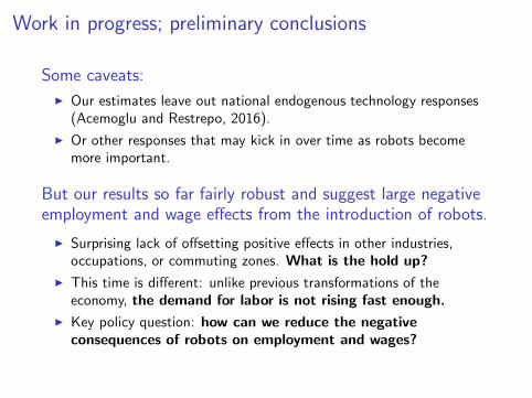
Work in progress; preliminary conclusions
Some caveats:
◮ Our estimates leave out national endogenous technology responses(Acemoglu and Restrepo, 2016).
◮ Or other responses that may kick in over time as robots becomemore important.
But our results so far fairly robust and suggest large negativeemployment and wage effects from the introduction of robots.
◮ Surprising lack of offsetting positive effects in other industries,occupations, or commuting zones. What is the hold up?
◮ This time is different: unlike previous transformations of theeconomy, the demand for labor is not rising fast enough.
◮ Key policy question: how can we reduce the negative
consequences of robots on employment and wages?

Additional results: full placebo estimates
Table: Placebo test that explores if the exposure to robots is related to pastchanges in employment from 1970 to 1990.
(1) (2) (3) (4) (5) (6)
Panel A. Census private employment to population ratio (1970-1990).
Change in exposure to robots from 1993 to2007
-0.001 -0.001 0.001 0.001 -0.005 -0.001(0.003) (0.002) (0.002) (0.002) (0.003) (0.005)
Observations 722 722 722 722 718 714Panel B. log of hourly wages (1970-1990).
Change in exposure to robots from 1993 to2007
-0.014∗ -0.013∗ -0.004 0.003 -0.002 0.018(0.007) (0.007) (0.008) (0.008) (0.007) (0.015)
Observations 96487 96487 96487 96487 94804 95109Covariates & sample restrictions:Census division dummies X X X X X X
Demographics X X X X X
Broad industry shares X X X X
Trade and routinization X X X
Down-weights outliers X
Removes highly exposed areas X
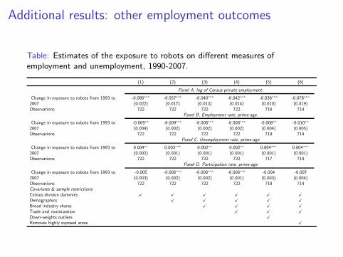
Additional results: other employment outcomes
Table: Estimates of the exposure to robots on different measures ofemployment and unemployment, 1990-2007.
(1) (2) (3) (4) (5) (6)
Panel A. log of Census private employment.
Change in exposure to robots from 1993 to2007
-0.086∗∗∗ -0.057∗∗∗ -0.040∗∗∗ -0.042∗∗∗ -0.036∗∗∗ -0.078∗∗∗
(0.022) (0.017) (0.013) (0.014) (0.010) (0.019)Observations 722 722 722 722 716 714
Panel B. Employment rate, prime-age.
Change in exposure to robots from 1993 to2007
-0.009∗∗ -0.009∗∗∗ -0.008∗∗∗ -0.008∗∗∗ -0.008∗∗ -0.010∗∗
(0.004) (0.002) (0.002) (0.002) (0.004) (0.005)Observations 722 722 722 722 719 714
Panel C. Unemployment rate, prime-age
Change in exposure to robots from 1993 to2007
0.004∗∗ 0.003∗∗∗ 0.002∗∗ 0.002∗∗ 0.004∗∗∗ 0.004∗∗∗
(0.002) (0.001) (0.001) (0.001) (0.001) (0.001)Observations 722 722 722 722 717 714
Panel D. Participation rate, prime-age
Change in exposure to robots from 1993 to2007
-0.005 -0.006∗∗∗ -0.006∗∗∗ -0.006∗∗∗ -0.004 -0.007(0.003) (0.002) (0.002) (0.001) (0.003) (0.004)
Observations 722 722 722 722 718 714Covariates & sample restrictions:Census division dummies X X X X X X
Demographics X X X X X
Broad industry shares X X X X
Trade and routinization X X X
Down-weights outliers X
Removes highly exposed areas X
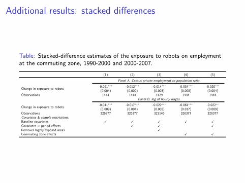
Additional results: stacked differences
Table: Stacked-difference estimates of the exposure to robots on employmentat the commuting zone, 1990-2000 and 2000-2007.
(1) (2) (3) (4) (5)
Panel A. Census private employment to population ratio.
Change in exposure to robots-0.021∗∗∗ -0.012∗∗∗ -0.014∗∗∗ -0.034∗∗∗ -0.020∗∗∗
(0.004) (0.002) (0.003) (0.008) (0.004)Observations 1444 1444 1429 1444 1444
Panel B. log of hourly wages.
Change in exposure to robots-0.041∗∗∗ -0.017∗∗∗ -0.022∗∗∗ -0.061∗∗∗ -0.022∗∗
(0.009) (0.004) (0.008) (0.017) (0.009)Observations 326377 326377 323146 326377 326377Covariates & sample restrictions:Baseline covariates X X X X X
Covariates × period effects X X X
Removes highly exposed areas X
Commuting zone effects X X
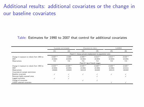
Additional results: additional covariates or the change in
our baseline covariates
Table: Estimates for 1990 to 2007 that control for additional covariates
Lagged outcomes Change in covs. LASSO
(1) (2) (3) (4) (5) (6)
Panel A. Census private employment to population ratio.
Change in exposure to robots from 1993 to2007
-0.007∗∗∗ -0.008∗ -0.009∗∗∗ -0.013∗∗∗ -0.012∗∗∗ -0.018∗∗∗
(0.002) (0.004) (0.002) (0.004) (0.003) (0.004)Observations 722 714 722 714 722 714
Panel B. log of hourly wages.
Change in exposure to robots from 1993 to2007
-0.023∗∗∗ -0.029∗∗∗ -0.025∗∗∗ -0.028∗∗∗ -0.026∗∗∗ -0.025∗∗
(0.004) (0.005) (0.004) (0.006) (0.006) (0.011)Observations 134404 132624 163114 161042 163114 161042Covariates & sample restrictions:Baseline covariates X X X X X X
Removes highly exposed areas X X X
Lagged outcomes X X
Change of covariates X X
LASSO selected covariates X X
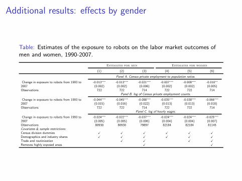
Additional results: effects by gender
Table: Estimates of the exposure to robots on the labor market outcomes ofmen and women, 1990-2007.
Estimates for men Estimates for women
(1) (2) (3) (4) (5) (6)
Panel A. Census private employment to population ratios.
Change in exposure to robots from 1993 to2007
-0.013∗∗∗ -0.013∗∗∗ -0.021∗∗∗ -0.007∗∗∗ -0.008∗∗∗ -0.010∗∗
(0.002) (0.002) (0.006) (0.002) (0.002) (0.005)Observations 722 722 714 722 722 714
Panel B. log of Census private employment counts.
Change in exposure to robots from 1993 to2007
-0.044∗∗∗ -0.045∗∗∗ -0.088∗∗∗ -0.035∗∗∗ -0.038∗∗∗ -0.066∗∗∗
(0.015) (0.016) (0.022) (0.013) (0.013) (0.018)Observations 722 722 714 722 722 714
Panel C. log of hourly wages.
Change in exposure to robots from 1993 to2007
-0.024∗∗∗ -0.022∗∗∗ -0.037∗∗∗ -0.024∗∗∗ -0.024∗∗∗ -0.025∗∗∗
(0.005) (0.005) (0.006) (0.004) (0.004) (0.007)Observations 80930 80930 79897 82184 82184 81145Covariates & sample restrictions:Census division dummies X X X X X X
Demographics and industry shares X X X X X X
Trade and routinization X X X X
Removes highly exposed areas X X
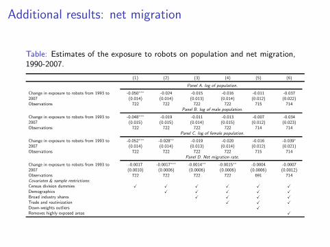
Additional results: net migration
Table: Estimates of the exposure to robots on population and net migration,1990-2007.
(1) (2) (3) (4) (5) (6)
Panel A. log of population.
Change in exposure to robots from 1993 to2007
-0.050∗∗∗ -0.024 -0.015 -0.016 -0.011 -0.037(0.014) (0.014) (0.013) (0.014) (0.012) (0.022)
Observations 722 722 722 722 715 714Panel B. log of male population.
Change in exposure to robots from 1993 to2007
-0.048∗∗∗ -0.019 -0.011 -0.013 -0.007 -0.034(0.015) (0.015) (0.014) (0.015) (0.012) (0.023)
Observations 722 722 722 722 714 714Panel C. log of female population.
Change in exposure to robots from 1993 to2007
-0.052∗∗∗ -0.028∗∗ -0.019 -0.020 -0.016 -0.039∗
(0.014) (0.014) (0.013) (0.014) (0.012) (0.021)Observations 722 722 722 722 715 714
Panel D. Net migration rate.
Change in exposure to robots from 1993 to2007
-0.0017 -0.0017∗∗∗ -0.0014∗∗ -0.0015∗∗ -0.0004 -0.0007(0.0010) (0.0006) (0.0006) (0.0006) (0.0006) (0.0012)
Observations 722 722 722 722 691 714Covariates & sample restrictions:Census division dummies X X X X X X
Demographics X X X X X
Broad industry shares X X X X
Trade and routinization X X X
Down-weights outliers X
Removes highly exposed areas X
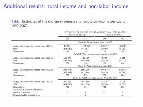
Additional results: total income and non-labor income
Table: Estimates of the change in exposure to robots on income per capita,1990-2007.
Estimates for income and transfers from 1990 to 2007
Change in levels Change in logs
(1) (2) (3) (4)
Panel A. Total income from the IRS
Change in exposure to robots from 1993 to2007
85.154 -170.963 -0.021∗∗∗ -0.028∗∗
(284.637) (413.671) (0.007) (0.012)Observations 722 714 722 714
Panel B. Total non-wage income from the IRS
Change in exposure to robots from 1993 to2007
190.476 20.637 0.008 0.015(118.649) (185.896) (0.013) (0.022)
Observations 722 714 722 714Panel C. Total income from the BEA
Change in exposure to robots from 1993 to2007
-985.376∗ -1686.296∗∗ -0.040∗∗∗ -0.049∗∗∗
(563.588) (812.698) (0.010) (0.015)Observations 722 714 722 714
Panel C. Total non-wage income from the BEA
Change in exposure to robots from 1993 to2007
250.025 441.995 -0.001 0.008(404.350) (711.930) (0.020) (0.037)
Observations 722 714 721 713Covariates & sample restrictions:Baseline covariates X X X X
Removes highly exposed areas X X
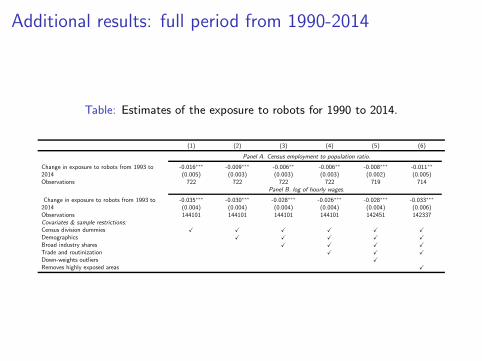
Additional results: full period from 1990-2014
Table: Estimates of the exposure to robots for 1990 to 2014.
(1) (2) (3) (4) (5) (6)
Panel A. Census employment to population ratio.
Change in exposure to robots from 1993 to2014
-0.016∗∗∗ -0.009∗∗∗ -0.006∗∗ -0.006∗∗ -0.008∗∗∗ -0.011∗∗
(0.005) (0.003) (0.003) (0.003) (0.002) (0.005)Observations 722 722 722 722 719 714
Panel B. log of hourly wages.
Change in exposure to robots from 1993 to2014
-0.035∗∗∗ -0.030∗∗∗ -0.028∗∗∗ -0.026∗∗∗ -0.028∗∗∗ -0.033∗∗∗
(0.004) (0.004) (0.004) (0.004) (0.004) (0.006)Observations 144101 144101 144101 144101 142451 142337Covariates & sample restrictions:Census division dummies X X X X X X
Demographics X X X X X
Broad industry shares X X X X
Trade and routinization X X X
Down-weights outliers X
Removes highly exposed areas X
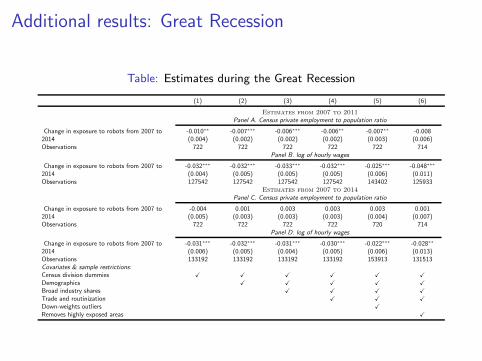
Additional results: Great Recession
Table: Estimates during the Great Recession
(1) (2) (3) (4) (5) (6)
Estimates from 2007 to 2011
Panel A. Census private employment to population ratio
Change in exposure to robots from 2007 to2014
-0.010∗∗ -0.007∗∗∗ -0.006∗∗∗ -0.006∗∗ -0.007∗∗ -0.008(0.004) (0.002) (0.002) (0.002) (0.003) (0.006)
Observations 722 722 722 722 722 714Panel B. log of hourly wages
Change in exposure to robots from 2007 to2014
-0.032∗∗∗ -0.032∗∗∗ -0.033∗∗∗ -0.032∗∗∗ -0.025∗∗∗ -0.048∗∗∗
(0.004) (0.005) (0.005) (0.005) (0.006) (0.011)Observations 127542 127542 127542 127542 143402 125933
Estimates from 2007 to 2014
Panel C. Census private employment to population ratio
Change in exposure to robots from 2007 to2014
-0.004 0.001 0.003 0.003 0.003 0.001(0.005) (0.003) (0.003) (0.003) (0.004) (0.007)
Observations 722 722 722 722 720 714Panel D. log of hourly wages
Change in exposure to robots from 2007 to2014
-0.031∗∗∗ -0.032∗∗∗ -0.031∗∗∗ -0.030∗∗∗ -0.022∗∗∗ -0.028∗∗
(0.006) (0.005) (0.004) (0.005) (0.006) (0.013)Observations 133192 133192 133192 133192 153913 131513Covariates & sample restrictions:Census division dummies X X X X X X
Demographics X X X X X
Broad industry shares X X X X
Trade and routinization X X X
Down-weights outliers X
Removes highly exposed areas X
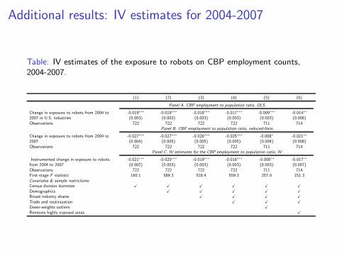
Additional results: IV estimates for 2004-2007
Table: IV estimates of the exposure to robots on CBP employment counts,2004-2007.
(1) (2) (3) (4) (5) (6)
Panel A. CBP employment to population ratio, OLS.
Change in exposure to robots from 2004 to2007 in U.S. industries
-0.019∗∗∗ -0.019∗∗∗ -0.018∗∗∗ -0.017∗∗∗ -0.009∗∗∗ -0.014∗∗
(0.003) (0.003) (0.003) (0.003) (0.003) (0.006)Observations 722 722 722 722 711 714
Panel B. CBP employment to population ratio, reduced-form.
Change in exposure to robots from 2004 to2007
-0.027∗∗∗ -0.027∗∗∗ -0.026∗∗∗ -0.025∗∗∗ -0.008∗ -0.021∗∗
(0.004) (0.005) (0.005) (0.005) (0.004) (0.008)Observations 722 722 722 722 711 714
Panel C. IV estimates for the CBP employment to population ratio, IV.
Instrumented change in exposure to robotsfrom 2004 to 2007
-0.021∗∗∗ -0.020∗∗∗ -0.019∗∗∗ -0.018∗∗∗ -0.008∗∗ -0.017∗∗
(0.002) (0.003) (0.003) (0.003) (0.003) (0.007)Observations 722 722 722 722 711 714First-stage F statistic 160.1 589.3 518.4 559.3 257.0 151.3Covariates & sample restrictions:Census division dummies X X X X X X
Demographics X X X X X
Broad industry shares X X X X
Trade and routinization X X X
Down-weights outliers X
Removes highly exposed areas X


