Robust and LPV control of MIMO systems Part 3: Robustness ...o.sename/docs/robusta.pdf · Robust...

Robust and LPV control of MIMO systemsPart 3: Robustness analysis

Olivier Sename

GIPSA-Lab

Tecnologico de Monterrey, July 2016

Olivier Sename (GIPSA-Lab) Robust and LPV control - part 3 Tecnologico de Monterrey, July 2016 1 / 28

1. Introduction

2. Representation of uncertainties

3. Definition of Robustness analysis

4. Robustness analysis: the unstructured case

5. Robustness analysis: the structured case

6. Robust control design

O. Sename [GIPSA-lab] 2/28

Introduction

Introduction

• A control system is robust if it is insensitive to differences between the actual system and themodel of the system which was used to design the controller

• How to take into account the difference between the actual system and the model ?• A solution: using a model set BUT : very large problem and not exact yet

A method: these differences are referred as model uncertainty.The approach

1 determine the uncertainty set: mathematical representation2 check Robust Stability3 check Robust Performance

Lots of forms can be derived according to both our knowledge of the physical mechanism thatcause the uncertainties and our ability to represent these mechanisms in a way that facilitatesconvenient manipulation.Several origins :

• Approximate knowledge and variations of some parameters• Measurement imperfections (due to sensor)• At high frequencies, even the structure and the model order is unknown (100• Choice of simpler models for control synthesis• Controller implementation

Two classes: parametric uncertainties / neglected or unmodelled dynamics


Representation of uncertainties

Example 1: uncertainties

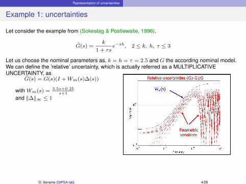
Let consider the example from (Sokestag & Postlewaite, 1996).

G(s) =k

1 + τse−sh, 2 ≤ k, h, τ ≤ 3

Let us choose the nominal parameters as, k = h = τ = 2.5 and G the according nominal model.We can define the ’relative’ uncertainty, which is actually referred as a MULTIPLICATIVEUNCERTAINTY, as


G(s) = G(s)(I +Wm(s)∆(s))

with Wm(s) = 3.5s+0.25s+1

and ‖∆‖∞ ≤ 1


Example 2: unmodelled dynamcis


10-8 10-6 10-4 10-2 100 102 104-250

-200

-150

-100

-50

0

Mag

nitu

de (

dB)

Bode Diagram

Frequency (rad/s)

(Greal-Gnom)/Gnom

Wm

Let us consider the system:

G(s) = G(s)1

1 + τs, τ ≤ τmax

This can be modelled as:

G(s) = G0(s)(I +Wm(s)∆(s))

with Wm(s) = τmaxjω1+τmaxjω

and ‖∆‖∞ ≤ 1

This can be represented as

with

N(s) =

[N11(s) N12(s)N21(s) N22(s)

]=

(0 I

G0Wm(s) G0(s)

)


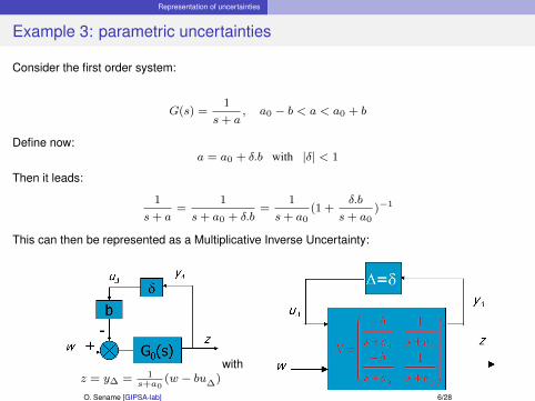
Example 3: parametric uncertainties

Consider the first order system:

G(s) =1

s+ a, a0 − b < a < a0 + b

Define now:a = a0 + δ.b with |δ| < 1

Then it leads:

1

s+ a=

1

s+ a0 + δ.b=

1

s+ a0(1 +

δ.b

s+ a0)−1

This can then be represented as a Multiplicative Inverse Uncertainty:


withz = y∆ = 1

s+a0(w − bu∆)


Example 3 (cont.) same example with state space formulation

Let us first the transfer function G(s) = 1s+a

as

G :

{x = (−a0 − δ.b)x+ wz = x

(1)

In order to use an LFT, let us define the uncertain input:

u∆ = δx,

Then the previous system can be rewritten in the following LFR:


where ∆ and y∆ are given as:

∆ =[δ], y∆ = (x)

and N given by the state space representation:

N :

x = −a0x− bu∆ + wy∆ = xz = x

(2)


Example 4: parametric uncertainties in state space equations

Let us consider the following uncertain system:

G :

x1 = (−2 + δ1)x1 + (−3 + δ2)x2

x2 = (−1 + δ3)x2 + uy = x1

(3)

In order to use an LFT, let us define the uncertain inputs:

u∆1= δ1x1, u∆2

= δ2x2, u∆3= δ3x2

Then the previous system can be rewritten in the following LFR:


where ∆ and y∆ are given as:

∆ =

δ1 0 00 δ2 00 0 δ3

, y∆ =

x1

x2

x2

and N given by the state space representation:

N :

x1

x2

==

−2x1 − 3x2 + u∆1+ u∆2

−x2 + u+ u∆3

y = x1

(4)


Towards LFR (LFT)

The previous computations are in fact the first step towards an unified representation of theuncertainties: the Linear Fractional Representation (LFR).Indeed the previous schemes can be rewritten in the following general representation as:

Figure: N∆ structure

This LFR gives then the transfer matrix from w to z, and is referred to as the upper LinearFractional Transformation (LFT) :

Fu(N,∆) = N22 +N21∆(I −N11∆)−1N12

This LFT exists and is well-posed if (I −N11∆)−1 is invertible



LFT definition

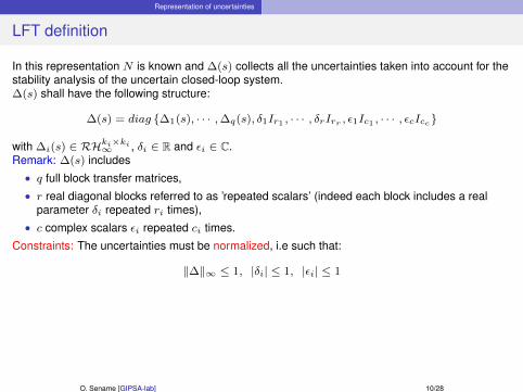
In this representation N is known and ∆(s) collects all the uncertainties taken into account for thestability analysis of the uncertain closed-loop system.∆(s) shall have the following structure:

∆(s) = diag {∆1(s), · · · ,∆q(s), δ1Ir1 , · · · , δrIrr , ε1Ic1 , · · · , εcIcc}

with ∆i(s) ∈ RHki×ki∞ , δi ∈ R and εi ∈ C.Remark: ∆(s) includes

• q full block transfer matrices,• r real diagonal blocks referred to as ’repeated scalars’ (indeed each block includes a real

parameter δi repeated ri times),• c complex scalars εi repeated ci times.

Constraints: The uncertainties must be normalized, i.e such that:

‖∆‖∞ ≤ 1, |δi| ≤ 1, |εi| ≤ 1



Uncertainty types

We have seen in the previous examples the two important classes of uncertainties, namely:• UNSTRUCTURED UNCERTAINTIES: we ignore the structure of ∆, considered as a full

complex perturbation matrix, such that ‖∆‖∞ ≤ 1.We then look at the maximal admissible norm for ∆, to get Robust Stability and Performance.This will give a global sufficient condition on the robustness of the control scheme.This may lead to conservative results since all uncertainties are collected into a single matrixignoring the specific role of each uncertain parameter/block.

• STRUCTURED UNCERTAINTIES: we take into account the structure of ∆, (always such that‖∆‖∞ ≤ 1).The robust analysis will then be carried out for each uncertain parameter/block.This needs to introduce a new tool: the Structured Singular Value. We then can obtain morefine results but using more complex tools.

The analysis is provided in what follows for both cases.In Matlabthis analysis is provided in the tools robuststab and robustperf.


Definition of Robustness analysis

Robustness analysis: problem formulation

Since the analysis will be carried you for a closed-loop system, N should be defined as theconnection of the plant and the controller. Therefore, in the framework of the H∞ control, thefollowing extended General Control Configuration is considered:

Figure: P − K − ∆ structure

and N is such that

N = Fl(P,K)



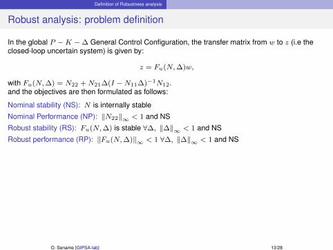
Robust analysis: problem definition

In the global P −K −∆ General Control Configuration, the transfer matrix from w to z (i.e theclosed-loop uncertain system) is given by:

z = Fu(N,∆)w,

with Fu(N,∆) = N22 +N21∆(I −N11∆)−1N12.and the objectives are then formulated as follows:

Nominal stability (NS): N is internally stable

Nominal Performance (NP): ‖N22‖∞ < 1 and NS

Robust stability (RS): Fu(N,∆) is stable ∀∆, ‖∆‖∞ < 1 and NS

Robust performance (RP): ‖Fu(N,∆)‖∞ < 1 ∀∆, ‖∆‖∞ < 1 and NS



Towards Robust stability analysis

Robust Stability= with a given controller K, we determine wether the system remains stable for allplants in the uncertainty set.According to the definition of the previous upper LFT, when N is stable, the instability may onlycome from (I −N11∆). Then it is equivalent to study the M −∆ structure, given as:

Figure: M − ∆ structure

This leads to the definition of the Small Gain Theorem

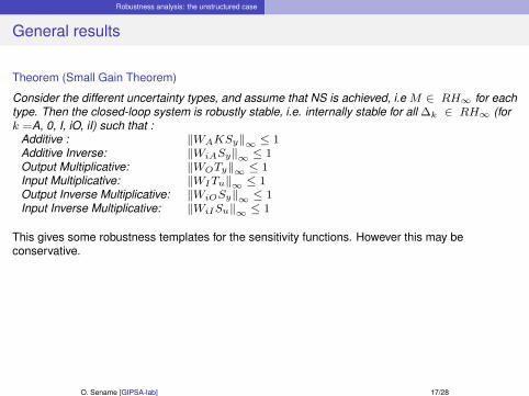
Theorem (Small Gain Theorem)

Suppose M ∈ RH∞. Then the closed-loop system in Fig. 3 is well-posed and internally stablefor all ∆ ∈ RH∞ such that :

‖∆‖∞ ≤ δ(resp. < δ) if and only if ‖M(s)‖∞ < 1/δ(resp. ‖M(s)‖∞ ≤ 1)


Robustness analysis: the unstructured case

Definition of the uncertainty types

Figure: 6 uncertainty representations



Robust stability analysis: additive case

Objective: applying the Small Gain Theorem to these unstructured uncertainty representations.


Let us consider the following simple controlscheme as:

Figure: Control scheme

The objective is to obtain:

Additive case:G(s) = G(s) +WA(s)∆A(s).Computing the N −∆ form gives

N(s) =

(−WAKSy WAKSy

Sy Ty

)Output Multiplicative uncertainties:G(s) = (I +WO(s)∆O(s))G(s).Then it leads

N(s) =

(−WOTy WOTySy Ty

)


General results

Theorem (Small Gain Theorem)

Consider the different uncertainty types, and assume that NS is achieved, i.e M ∈ RH∞ for eachtype. Then the closed-loop system is robustly stable, i.e. internally stable for all ∆k ∈ RH∞ (fork =A, 0, I, iO, iI) such that :

Additive : ‖WAKSy‖∞ ≤ 1Additive Inverse: ‖WiASy‖∞ ≤ 1Output Multiplicative: ‖WOTy‖∞ ≤ 1Input Multiplicative: ‖WITu‖∞ ≤ 1Output Inverse Multiplicative: ‖WiOSy‖∞ ≤ 1Input Inverse Multiplicative: ‖WiISu‖∞ ≤ 1

This gives some robustness templates for the sensitivity functions. However this may beconservative.



Illustration on the SISO case

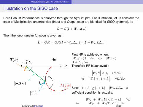
Here Robust Stability is analyzed through the Nyquist plot. For illustration, let us consider the caseof Multiplicative uncertainties (Input and Output case are identical for SISO systems), i.e

G = G(I +Wm∆m)

Then the loop transfer function is given as:

L = GK = GK(I +Wm∆m) = L+WmL∆m;


According to the Nyquist theorem, RS isachieved the the closed-loop system isstable for any L should not encircle, i.e Lshould not encircle -1 for all uncertainties.According to the figure, a sufficient conditionis then:

|WmL| < |1 + L| , ∀ω⇔∣∣∣WmL

1+L

∣∣∣ < 1, ∀ω⇔ |WmT | < 1 ∀ω


A first insight in Robust Performance

Objective: applying the Small Gain Theorem to these unstructured uncertainty representations.


Let us consider the following simple controlscheme as:

Figure: Control scheme

Case of Output Multiplicative uncertainties:G(s) = (I +WO(s)∆O(s))G(s).Computing the N −∆ form gives

N(s) =

[N11(s) N12(s)N21(s) N22(s)

]=

(−WOTy WOTy−WeSy WeSy

)

We wish to get:The objectives are then formulated asfollows:

NS: N is internally stable

NP: ‖WeSy‖∞ < 1 and NS

RS: ‖WOTy‖∞ < 1 and NS

RP: ‖Fu(N,∆)‖∞ < 1 ∀∆, ‖∆‖∞ < 1,Sufficient condition: NS andσ(WOTy) + σ(WeSy) < 1, ∀ω


Illustration on the SISO case

Here Robust Performance is analyzed through the Nyquist plot. For illustration, let us consider thecase of Multiplicative uncertainties (Input and Output case are identical for SISO systems), i.e

G = G(I +Wm∆m)

Then the loop transfer function is given as:

L = GK = GK(I +Wm∆m) = L+WmL∆m;


First NP is achieved when:|WeS| < 1 ∀ω, ⇔ |We| <|1 + L| , ∀ω.Therefore RP is achieved if∣∣∣WeS

∣∣∣ < 1, ∀S,∀ω

⇔ |We| <∣∣∣1 + L

∣∣∣ , ∀L, ∀ωSince

∣∣∣1 + L∣∣∣ ≥ |1 + L| − |WmL∆m|, a

sufficient condition is actually:

|We|+ |WmL| < |1 + L| , ∀ω⇔ |WeS|+ |WmT | < 1, ∀ω

Robustness analysis: the structured case

The structured case

∆ = {diag{∆1, · · · ,∆q , δ1Ir1 , · · · , δrIrr , ε1Ic1 , · · · , εcIcc} ∈ Ck×k} (5)

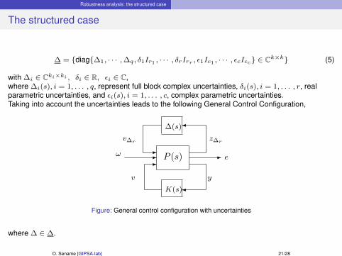
with ∆i ∈ Cki×ki , δi ∈ R, εi ∈ C,where ∆i(s), i = 1, . . . , q, represent full block complex uncertainties, δi(s), i = 1, . . . , r, realparametric uncertainties, and εi(s), i = 1, . . . , c, complex parametric uncertainties.Taking into account the uncertainties leads to the following General Control Configuration,

�

---

�

-

∆(s)

K(s)

y

e

z∆r

ω

v

P (s)

v∆r

Figure: General control configuration with uncertainties

where ∆ ∈ ∆.



The structured singular value

To handle parametric uncertainties, we need to introduce µ, the structured singular value, definedas:

Definition (µ)

For M ∈ Cn×n, the structure singular value is defined as:

µ∆(M) :=1

min{σ(∆) : ∆ ∈ ∆, det(I −∆M) 6= 0}

In other words, it allows to find the smallest structured ∆ which makes det(I −M∆) = 0.

Theorem (The structured Small Gain Theorem)

Let M(s) be a MIMO LTI stable system and ∆(s) a LTI uncertain stable matrix, (i.e. ∈ RH∞).The system in Fig. 3 is stable for all ∆(s) in (5) if and only if:

∀ω ∈ R µ∆ (M(jω)) ≤ 1, with M(s) := Nzv(s)

More generally both following statements are equivalent• For µ ∈ R, N(s) and ∆(s) belong to RH∞, and

∀ω ∈ R, µ∆ (M(jω)) ≤ µ

• the system represented in figure 3 is stable for any uncertainty ∆(s) of the form (5) such that :

||∆(s)| |∞ < 1/µO. Sename [GIPSA-lab] 22/28


Build the whole control scheme



Introduction of a fictive block

Usually only real parametric uncertainties (given in ∆r) are considered for RS analysis. RPanalysis also needs a fictive full block complex uncertainty, as below,

- -

-

�

?

�∆f

∆(s)

∆r

N(s)ω e

v∆rz∆r

N(s)

Figure: N∆

where N(s) =

[N11(s) N12(s)N21(s) N22(s)

], and the closed-loop transfer matrix is:

Tew(s) = N22(s) +N21(s)∆(s)(I −N11(s))−1N12(s) (6)



Robust analysis theorem

For RS, we shall determine how large ∆ (in the sense of H∞) can be without destabilizing thefeedback system. From (6), the feedback system becomes unstable if det(I −N11(s) = 0 forsome s ∈ C,<(s) ≥ 0. The result is then the following.

Theorem ([?])

Assume that the nominal system New and the perturbations ∆ are stable. Then the feedbacksystem is stable for all allowed perturbations ∆ such that ||∆(s)| |∞ < 1/β if and only if∀ω ∈ R, µ∆ (N11(jω)) ≤ β.

Assuming nominal stability, RS and RP analysis for structured uncertainties are therefore suchthat:

NP ⇔ σ(N22) = µ∆f(N22) ≤ 1, ∀ω

RS ⇔ µ∆r (N11) < 1, ∀ω

RP ⇔ µ∆(N) < 1, ∀ω, ∆ =

[∆f 00 ∆r

]Finally, let us remark that the structured singular value cannot be explicitly determined, so that themethod consists in calculating an upper bound and a lower bound, as closed as possible to µ.



Summary

The steps to be followed in the RS/RP analysis for structured uncertainties are then:• Definition of the real uncertainties ∆r and of the weighting functions• Evaluation of µ(N22)∆f

, µ(N11)∆rand µ(N)∆

• Computation of the admissible intervals for each parameter

Remark: The Robust Performance analysis is quite conservative and requires a tight definition ofthe weighting functions that do represent the performance objectives to be satisfied by theuncertain closed-loop system. Therefore it is necessary to distinguish the weighting functionsused for the nominal design from the ones used for RP analysis.


Robust design

Outline

1. Introduction

2. Representation of uncertainties

3. Definition of Robustness analysis

4. Robustness analysis: the unstructured case

5. Robustness analysis: the structured case

6. Robust control design


Robust design

Brief overview

In order to design a robust control, i.e. a controller for which the synthesis actually accounts foruncertainties, some of the methods are:

• Unstructured uncertainties: Consider an uncertainty weight (unstructured form), andinclude the Small Gain Condition through a new controlled output. For example, robustnessface to Ouptut Multiplicative Uncertainties can be considered into the design procedureadding the controlled output ey = WOy, which, when tracking performance is expected, leadsto the condition ‖WOTy ‖∞≤ 1.

• Structured uncertainties: the design of a robust controller in the presence of suchuncertainties is the µ− synthesis. It is handled through an interactive procedure, referred toas the DK iteration. This procedure is much more involved than a "simple" H∞ controldesign and often leads to an increase of the order of the controller (which is already the sumof the order of the plant and of the weighting functions).

• Use other mathematical representation of parametric uncertainties, [?], as for instance thepolytopic model. In that case the set of uncertain parameters is assumed to be a polytope(i.e. a convex) set. The stability issue in that framework is referred to as the ’Quadraticstability’ i.e find a single Lyapunov function for the uncertainty set. While in the general casethis is an unbounded problem, in the polytopic case (or in the affine case), the stability is to beanalyzed only at the vertices of the polytope, which is a finite dimensional problem.This approach can then be applied to find a single controller, valid over the potyopic set. Notethat this approach gives rise to the LPV design for polytopic systems, as described next.


Date post:	23-May-2018
Category:	Documents
Upload:	dinhnhi
View:	215 times
Download:	0 times

Robust and LPV control of MIMO systems Part 3: Robustness ...o.sename/docs/robusta.pdf · Robust...

Documents