Journal of Machine Learning Research 18 (2017) 1-40 Submitted 12/16; Revised 11/17; Published 12/17 Robust and Scalable Bayes via a Median of Subset Posterior Measures Stanislav Minsker [email protected]Department of Mathematics University of Southern California Los Angeles, CA 90089, USA Sanvesh Srivastava [email protected]Department of Statistics and Actuarial Science University of Iowa Iowa City, IA 52242, USA Lizhen Lin [email protected]Department of Applied and Computational Mathematics and Statistics The University of Notre Dame Notre Dame, IN 46556, USA David B. Dunson [email protected]Departments of Statistical Science, Mathematics, and ECE Duke University Durham, NC 27708, USA Editor: David Blei Abstract We propose a novel approach to Bayesian analysis that is provably robust to outliers in the data and often has computational advantages over standard methods. Our technique is based on splitting the data into non-overlapping subgroups, evaluating the posterior distribution given each independent subgroup, and then combining the resulting measures. The main novelty of our approach is the proposed aggregation step, which is based on the evaluation of a median in the space of probability measures equipped with a suitable collection of distances that can be quickly and efficiently evaluated in practice. We present both theoretical and numerical evidence illustrating the improvements achieved by our method. Keywords: Big data, geometric median, distributed computing, parallel MCMC, Wasser- stein distance 1. Introduction Contemporary data analysis problems pose several general challenges. One is resource limitations: massive data require computer clusters for storage and processing. Another problem occurs when data are severely contaminated by “outliers” that are not easily iden- c 2017 Stanislav Minsker, Sanvesh Srivastava, Lizhen Lin and David B. Dunson. License: CC-BY 4.0, see https://creativecommons.org/licenses/by/4.0/. Attribution requirements are provided at http://jmlr.org/papers/v18/16-655.html.
Transcript
Journal of Machine Learning Research 18 (2017) 1-40 Submitted 12/16; Revised 11/17; Published 12/17
Robust and Scalable Bayes via a Median of Subset PosteriorMeasures
Stanislav Minsker [email protected] of MathematicsUniversity of Southern CaliforniaLos Angeles, CA 90089, USA
Sanvesh Srivastava [email protected] of Statistics and Actuarial ScienceUniversity of IowaIowa City, IA 52242, USA
Lizhen Lin [email protected] of Applied and Computational Mathematics and StatisticsThe University of Notre DameNotre Dame, IN 46556, USA
Departments of Statistical Science, Mathematics, and ECE
Duke University
Durham, NC 27708, USA
Editor: David Blei
Abstract
We propose a novel approach to Bayesian analysis that is provably robust to outliers inthe data and often has computational advantages over standard methods. Our techniqueis based on splitting the data into non-overlapping subgroups, evaluating the posteriordistribution given each independent subgroup, and then combining the resulting measures.The main novelty of our approach is the proposed aggregation step, which is based onthe evaluation of a median in the space of probability measures equipped with a suitablecollection of distances that can be quickly and efficiently evaluated in practice. We presentboth theoretical and numerical evidence illustrating the improvements achieved by ourmethod.
Contemporary data analysis problems pose several general challenges. One is resourcelimitations: massive data require computer clusters for storage and processing. Anotherproblem occurs when data are severely contaminated by “outliers” that are not easily iden-
tified and removed. Following Box and Tiao (1968), an outlier can be defined as “being anobservation which is suspected to be partially or wholly irrelevant because it is not generatedby the stochastic model assumed.” While the topic of robust estimation has occupied animportant place in the statistical literature for several decades and significant progress hasbeen made in the theory of point estimation, robust Bayesian methods are not sufficientlywell-understood.
Our main goal is to take a step towards solving these problems, proposing a general Bayesianapproach that is
(i) provably robust to the presence of outliers in the data without any specific assumptionson their distribution or reliance on preprocessing;
(ii) scalable to big data sets through allowing computational algorithms to be implementedin parallel for different data subsets prior to an efficient aggregation step.
The proposed approach consists in splitting the sample into disjoint parts, implementingMarkov chain Monte Carlo (MCMC) or another posterior sampling method to obtain drawsfrom each “subset posterior” in parallel, and then using these draws to obtain weightedsamples from the median posterior (or M-Posterior), a new probability measure which is a(properly defined) median of a collection of subset posterior distributions. We show that,despite the loss of “interactions” among the data in different groups, the final result stilladmits strong guarantees; moreover, splitting the data gives certain advantages in terms ofrobustness to outliers.
In particular, we demonstrate that the M-Posterior is a probability measure centered at the“robust” estimator of the unknown parameter, the associated credible sets are often of thesame “width” as the credible sets obtained from the usual posterior distribution and admitstrong “frequentist” coverage guarantees (see Section 3.2 for exact statements).
The paper is organized as follows: Section 1.1 contains an overview of the existing literatureand explains the goals that we aim to achieve in this work. Section 2 introduces themathematical background and key facts used throughout the paper. Section 3 describes themain theoretical results for the median posterior. Section 4 presents details of algorithms,implementation, and numerical performance of the median posterior for several models. Thesimulation study and analysis of data examples convincingly show the robustness propertiesof the median posterior. In particular, we have used M-Posterior for scalable nonparametricBayesian modeling of joint dependence in the multivariate categorical responses collectedby the General Social Survey (gss.norc.org). Proofs that are omitted in the main textare contained in the supplementary material.
1.1 Discussion of Related Work
A. Dasgupta remarks that (see the discussion following the work by Berger, 1994): “Exactlywhat constitutes a study of Bayesian robustness is of course impossible to define.” Thepopular definition which also indicates the main directions of research in this area is due toBerger (1994): “Robust Bayesian analysis is the study of the sensitivity of Bayesian answers
to uncertain inputs. These uncertain inputs are typically the model, prior distribution, orutility function, or some combination thereof.” Notable works on robustness of Bayesianprocedures to model misspecification include Doksum and Lo (1990) and Hoff (2007) thatinvestigate methods based on conditioning on partial information, as well as a more recentpaper by Miller and Dunson (2015) who introduced the notion of the “coarsened” posterior;however, its behavior in the presence of outliers is not explicitly addressed. Outliers aretypically accommodated by either employing heavy-tailed likelihoods (e.g., Svensen andBishop, 2005) or by attempting to identify and remove them as a first step (as in Boxand Tiao, 1968 or Bayarri and Berger, 1994). The common assumption in the Bayesianliterature is that the distribution of the outliers can be modeled (e.g., using a t-distribution,contamination by a larger variance parametric distribution, etc). In this paper, we insteadbypass the need to place a model on the outliers and do not require their removal priorto analysis; similar approach has previously been advocated by Hooker and Vidyashankar(2014). We base inference on the median posterior, whose robustness can be formally andprecisely quantified in terms of concentration properties around the true delta measureunder the potential influence of outliers and contaminations of arbitrary nature.
Also relevant is the recent progress in scalable Bayesian algorithms. Most methods designedfor distributed computing share a common feature: they efficiently use the data subsetavailable to a single machine and combine the “local” results for “global” learning, whileminimizing communication among cluster machines (Smola and Narayanamurthy, 2010). Awide variety of optimization-based approaches are available for distributed learning (Boydet al., 2011); however, the number of similar Bayesian methods is limited. One of thereasons for this limitation is that Bayesian approaches typically require an approximationto the full posterior distribution instead of just a point estimate of parameters.
Several major approaches exist for scalable Bayesian learning in a distributed setting. Thefirst approach independently evaluates the likelihood for each data subset across multiplemachines and returns the likelihoods to a “master” machine, where they are appropriatelycombined with the prior using conditional independence assumptions of the probabilisticmodel. These two steps are repeated at every MCMC iteration (see Smola and Narayana-murthy, 2010; Agarwal and Duchi, 2012). This approach is problem-specific and involvesextensive communication among machines. The second approach uses a so-called stochasticapproximation (SA) and successively learns “noisy” approximations to the full posterior dis-tribution using data in small mini-batches. A group of methods based on this approach usessampling-based techniques to explore the posterior distribution through modified Hamilto-nian or Langevin dynamics (e.g., Welling and Teh, 2011; Ahn et al., 2012; Korattikaraet al., 2013). Unfortunately, these methods fail to accommodate discrete-valued parametersand multimodality. Another subgroup of methods uses deterministic variational approxi-mations and learns the variational parameters of the approximated posterior through anoptimization-based approach (see Wang et al., 2011; Hoffman et al., 2013; Broderick et al.,2013). Although these techniques often have excellent predictive performance, it is wellknown (Bishop, 2006) that variational methods tend to substantially underestimate poste-rior uncertainty and provide a poor characterization of posterior dependence, while lackingtheoretical guarantees.
3
Minsker et al.
Our approach instead falls in a class of methods which avoid extensive communicationamong machines by running independent MCMC chains for each data subset and obtain-ing draws from subset posteriors. These subset posteriors can be combined in a variety ofways. Some of these methods simply average draws from each subset (Scott et al., 2013).Other alternatives use an approximation to the full posterior distribution based on kerneldensity estimates (Neiswanger et al., 2013) or the so-called Weierstrass transform (Wangand Dunson, 2013). These methods have limitations related to the dimension of the param-eter, moreover, their applicability and theoretical justification are restricted to parametricmodels. Unlike the method proposed below, none of the aforementioned algorithms areprovably robust. Another closely related method is the so-called WASP (Srivastava et al.,2015b). It is scalable but still lacks robustness guarantees.
Our work was inspired by recent multivariate median-based techniques for robust estimationdeveloped in Minsker (2015) (see also Hsu and Sabato, 2013; Alon et al., 1996; Lerasle andOliveira, 2011; Nemirovskiı and David, 1983 where similar ideas were applied in differentframeworks).
2. Preliminaries
We proceed by recalling key definitions and facts which will be used throughout the paper,followed by the definition of the M-Posterior distribution in Section 2.4.
2.1 Notation
In what follows, ‖ · ‖2 denotes the standard Euclidean distance in Rp and 〈·, ·〉Rp the asso-ciated dot product.
Given a totally bounded metric space (Y, d), the packing number M(ε,Y, d) is the maximalnumber N such that there exist N disjoint d-balls B1, . . . , BN of radius ε contained in Y,
i.e.,N⋃j=1
Bj ⊆ Y.
Let pθ, θ ∈ Θ be a family of probability density functions on Rp. Let l, u : Rp 7→ R+ betwo functions such that l(x) ≤ u(x) for every x ∈ Rp and d2(l, u) :=
∫Rp
(√u−√l)2(x)dx <∞.
A bracket [l, u] consists of all functions g : Rp 7→ R such that l(x) ≤ g(x) ≤ u(x) for allx ∈ Rp. For A ⊆ Θ, the bracketing number N[ ](ε,A, d) is defined as the smallest number
N such that there exist N brackets [li, ui], i = 1, . . . , N satisfying pθ, θ ∈ A ⊆N⋃i=1
[li, ui]
and d(li, ui) ≤ ε for all 1 ≤ i ≤ N .
For y ∈ Y, δy denotes the Dirac measure concentrated at y. In other words, for any Borel-measurable B, δy(B) = Iy ∈ B, where I· is the indicator function.
We will say that k : Y × Y 7→ R is a kernel if it is a symmetric, positive definite function.Assume that (H, 〈·, ·〉H) is a reproducing kernel Hilbert space (RKHS) of functions f : Y 7→
4
Robust and Scalable Bayes
R. Then k is a reproducing kernel for H if for any f ∈ H and y ∈ Y, 〈f, k(·, y)〉H = f(y)(see Aronszajn, 1950 for details).
For a square-integrable function f ∈ L2(Rp), f stands for its Fourier transform. For x ∈ R,bxc denotes the largest integer not greater than x.
Finally, given two nonnegative sequences an and bn, we write an . bn if an ≤ Cbnfor some C > 0 and all n. Other objects and definitions are introduced in the course ofexposition when necessity arises.
2.2 Generalizations of the Univariate Median
Let Y be a normed space with norm ‖ · ‖, and let µ be a probability measure on (Y, ‖ · ‖)equipped with Borel σ-algebra. Define the geometric median of µ by
x∗ = argminy∈Y
∫Y
(‖y − x‖ − ‖x‖)µ(dx).
In this paper, we focus on the special case when µ is a uniform distribution on a finitecollection of atoms x1, . . . , xm ∈ Y, so that
x∗ = medg(x1, . . . , xm) := argminy∈Y
m∑j=1
‖y − xj‖. (1)
The geometric median exists under rather general assumptions; for example, if Y is aHilbert space (this case will be our main focus; more general conditions were obtained byKemperman, 1987). Moreover, it is well-known that in this situation x∗ ∈ co(x1, . . . , xm)—
the convex hull of x1, . . . , xm (meaning that there exist nonnegative αj , j = 1 . . .m,m∑j=1
αj =
1 such that x∗ =m∑j=1
αjxj).
Another useful generalization of the univariate median is defined as follows. Let (Y, d) be ametric space with metric d, and x1, . . . , xk ∈ Y. Define B∗ to be the d-ball of minimal radiussuch that it is centered at one of x1, . . . , xm and contains at least half of these points.Then the median med0(x1, . . . , xm) of x1, . . . , xm is the center of B∗. In other words, let
ε∗ := infε > 0 : ∃j = j(ε) ∈ 1, . . . ,m and I(j) ⊂ 1, . . . ,m such that (2)
|I(j)| > m
2and ∀i ∈ I(j), d(xi, xj) ≤ 2ε
,
j∗ := j(ε∗), where ties are broken arbitrarily, and set
x∗ = med0(x1, . . . , xm) := xj∗ . (3)
We will say that x∗ is the metric median of x1, . . . , xm. Note that x∗ always belongs tox1, . . . , xm by definition. Advantages of this definition are its generality (only metricspace structure is assumed) and simplicity of numerical evaluation since only the pairwise
5
Minsker et al.
distances d(xi, xj), i, j = 1, . . . ,m are required to compute the median. This constructionwas previously employed by Nemirovskiı and David (1983) in the context of stochasticoptimization and is further studied by Hsu and Sabato (2013). A closely related notion ofthe median was used by Lopuhaa and Rousseeuw (1991) under the name of the “minimalvolume ellipsoid” estimator.
Finally, we recall an important property of the median (shared both by medg and med0)which states that it transforms a collection of independent, “weakly concentrated” estima-tors into a single estimator with significantly stronger concentration properties. Given q, αsuch that 0 < q < α < 1/2, define a nonnegative function ψ(α, q) via
ψ(α, q) := (1− α) log1− α1− q
+ α logα
q. (4)
The following result is an adaptation of Theorem 3.1 in (Minsker, 2015):
Theorem 1
a Assume that (H, ‖ · ‖) is a Hilbert space and θ0 ∈ H. Let θ1, . . . , θm ∈ H be a collectionof independent random variables. Let κ be a constant satisfying 0 ≤ κ < 1
3 . Supposeε > 0 is such that for all j, 1 ≤ j ≤ b(1− κ)mc+ 1,
Pr(‖θj − θ0‖ > ε
)≤ 1
7. (5)
Let θ∗ = medg(θ1, . . . , θm) be the geometric median of θ1, . . . , θm. Then
Pr(‖θ∗ − θ0‖ > 1.52ε
)≤[e
(1−κ)ψ(
3/7−κ1−κ ,1/7
)]−m.
b Assume that (Y, d) is a metric space and θ0 ∈ Y. Let θ1, . . . , θm ∈ Y be a collection ofindependent random variables. Let κ be a constant satisfying 0 ≤ κ < 1
3 . Supposeε > 0 is such that for all j, 1 ≤ j ≤ b(1− κ)mc+ 1,
Pr(d(θj , θ0) > ε
)≤ 1
4. (6)
Let θ∗ = med0(θ1, . . . , θm). Then
Pr(d(θ∗, θ0) > 3ε
)≤[e
(1−κ)ψ(
1/2−κ1−κ ,1/4
)]−m.
Proof See Section A.1 in the appendix.
Remark 2 While we require κ < 1/3 above for clarity and to keep the constants small, weprove a slightly more general result that holds for any κ < 1/2.
6
Robust and Scalable Bayes
Theorem 1 implies that the concentration of the geometric median of independent estimatorsaround the “true” parameter value improves geometrically fast with respect to the numberof such estimators, while the estimation rate is preserved, up to a constant. In our case, therole of θj ’s will be played by posterior distributions based on disjoint subsets of observations,viewed as elements of the space of signed measures equipped with a suitable distance.
Parameter κ allows taking corrupted observations into account: if the initial sample containsnot more than bκmc outliers (of arbitrary nature), then at most bκmc estimators amongstθ1, . . . , θm can be affected but their median remains stable, still being close to the unknownθ0 with high probability. To clarify the notion of “robustness” that such a statementprovides, assume that θ1, . . . , θm are consistent estimators of θ0 based on disjoint samplesof size n/m each. If n
m →∞, then κmn → 0, hence the breakdown point of the estimator θ∗
is 0 is general. However, it is able to handle a number of outliers that grows like o(n) whilepreserving consistency, which is the best one can hope for without imposing any additionalassumptions on the underlying distribution, parameter of interest or nature of the outliers.
Let us also mention that the the geometric median of a collection of points in a Hilbert spacebelongs to the convex hull of these points. Thus, one can think about “downweighing” someobservations (potential outliers) and increasing the weight of others, and geometric mediangives a way to formalize this approach. The median med0 defined in (3) corresponds to theextreme case when all but one weight are equal to 0. Its potential advantage lies in thefact that its evaluation requires only the knowledge of pairwise distances d(θi, θj), i, j =1, . . . ,m, see (2).
2.3 Distances Between Probability Measures
Next, we discuss the special family of distances between probability measures that will beused throughout the paper. These distances provide the necessary structure to define andevaluate medians in the space of measures, as discussed above. Since one of our goals wasto develop computationally efficient techniques, we focus on distances that admit accuratenumerical approximation.
Assume that (X, ρ) is a separable metric space, and let F = f : X 7→ R be a collection ofreal-valued functions. Given two Borel probability measures P,Q on X, define
‖P −Q‖F := supf∈F
∣∣∣∣∫Xf(x)d(P −Q)(x)
∣∣∣∣ . (7)
Important special cases include the situation when
F = FL := f : Θ 7→ R s.t. ‖f‖L ≤ 1, (8)
where ‖f‖L := supx1 6=x2
|f(x1)−f(x2)|ρ(x1,x2) is the Lipschitz constant of f .
It is well-known (Dudley, 2002, Theorem 11.8.2) that in this case ‖P − Q‖FL is equal tothe Wasserstein distance (also known as the Kantorovich-Rubinstein distance)
dW1,ρ(P,Q) = infEρ(X,Y ) : L(X) = P, L(Y ) = Q
, (9)
7
Minsker et al.
where L(Z) denotes the law of a random variable Z and the infimum on the right is takenover the set of all joint distributions of (X,Y ) with marginals P and Q.
Another fruitful structure emerges when F is a unit ball in a Reproducing Kernel HilbertSpace (H, 〈·, ·〉H) with a reproducing kernel k : X× X 7→ R. That is,
F = Fk := f : X 7→ R, ‖f‖H :=√〈f, f〉H ≤ 1. (10)
Let Pk := P is a probability measure,∫X√k(x, x)dP (x) < ∞, and assume that P,Q ∈
Pk. Theorem 1 proven by Sriperumbudur et al. (2010) implies that the correspondingdistance between measures P and Q takes the form
‖P −Q‖Fk =
∥∥∥∥∫Xk(x, ·)d(P −Q)(x)
∥∥∥∥H. (11)
It follows that P 7→∫X k(x, ·)dP (x) is an embedding of Pk into the Hilbert space H which
can be seen as an application of the “kernel trick” in our setting. The Hilbert space structureallows one to use fast numerical methods to approximate the geometric median, see Section4 below.
Remark 3 Note that when P and Q are discrete measures (e.g., P =N1∑j=1
βjδzj and Q =
N2∑j=1
γjδyj ), then
‖P −Q‖2Fk =
N1∑i,j=1
βiβjk(zi, zj)+ (12)
N2∑i,j=1
γiγjk(yi, yj)− 2
N1∑i=1
N2∑j=1
βiγjk(zi, yj).
In this paper, we will only consider characteristic kernels, which means that ‖P −Q‖Fk = 0if and only if P = Q. It follows from Theorem 7 in Sriperumbudur et al. (2010) that asufficient condition for k to be characteristic is its strict positive definiteness: we say thatk is strictly positive definite if it is bounded, measurable, and such that for all non-zerosigned Borel measures ν ∫∫
X×X
k(x, y)dν(x)dν(y) > 0.
When X = Rp, a simple sufficient criterion for the kernel k to be characteristic follows fromTheorem 9 in Sriperumbudur et al. (2010):
Proposition 4 Let X = Rp, p ≥ 1. Assume that k(x, y) = φ(x − y) for some bounded,continuous, integrable, positive-definite function φ : Rp 7→ R.
1. Let φ be the Fourier transform of φ. If |φ(x)| > 0 for all x ∈ Rp, then k is character-istic;
8
Robust and Scalable Bayes
2. If φ is compactly supported, then k is characteristic.
Remark 5 It is important to mention that in practical applications, we often deal withempirical measures based on a collection of MCMC samples from the posterior distribution.A natural question is the following: if P and Q are probability measures on RD and Pm,Qn are their empirical versions, what is the size of the error
em,n :=∣∣∣‖P −Q‖Fk − ‖Pm −Qn‖Fk ∣∣∣?
For i.i.d samples, a useful and favorable fact is that em,n often does not depend on D: underweak assumptions on kernel k, em,n has an upper bound of order m−1/2 + n−1/2 (that is,limm,n→∞ Pr
(em,n ≥ C(m−1/2 + n−1/2)
)can be made arbitrarily small by choosing C big
enough, see Corollary 12 in Sriperumbudur et al., 2009). On the other hand, the boundfor the (stronger) Wasserstein distance is not dimension-free and is of order m−1/(D+1) +n−1/(D+1). Similar error rates hold for empirical measures based on samples from Markovchains used to approximate invariant distributions, including MCMC samples (see Boissardand Le Gouic, 2014 and Fournier and Guillin, 2015).
If X is a separable Hilbert space with dot product 〈·, ·〉X and P1, P2 are probability measureswith ∫
X‖x‖XdPi(x) <∞, i = 1, 2,
it will be useful to assume that the class F is chosen such that the distance between themeasures is lower bounded by the distance between their means, namely∥∥∥∥∫
XxdP1(x)−
∫XxdP2(x)
∥∥∥∥X≤ C‖P1 − P2‖F (13)
for some absolute constant C > 0. Clearly, this holds if F contains the set of continuouslinear functionals L = x 7→ 〈u, x〉X , u ∈ X, ‖u‖X ≤ 1/C, since∥∥∥∥∫
XxdPi(x)
∥∥∥∥X
= sup‖u‖X≤1
∫X〈x, u〉X dPi(x), i = 1, 2.
In particular, this is true for the Wasserstein distance dW1,ρ(·, ·) defined with respect to themetric ρ such that ρ(x, y) ≥ c1‖x − y‖X. Next, we will state a simple sufficient conditionon the kernel k(·, ·) for (13) to hold for the unit ball Fk.
Proposition 6 Let X be a separable Hilbert space, k0 : X×X 7→ R - a characteristic kernel,and define
k(x, y) := k0(x, y) + 〈x, y〉X .
Then k is characteristic and satisfies (13) with C = 1.
Proof Let H1 and H2 be two reproducing kernel Hilbert spaces with kernels k1 and k2
respectively. It is well-known (e.g., Aronszajn, 1950) that the space corresponding to kernelk = k1 + k2 is
H = f = f1 + f2, f1 ∈ H1, f2 ∈ H2
9
Minsker et al.
with the norm ‖f‖2H = inf‖f1‖2H + ‖f2‖2H, f1 + f2 = f. Hence, the unit ball of H containsthe unit balls of H1 and H2, so that for any probability measures P,Q
‖P −Q‖Fk ≥ max(‖P −Q‖Fk1 , ‖P −Q‖Fk2
),
which easily implies the result.
The kernels of the form k(x, y) = k0(x, y)+〈x, y〉X will prove especially useful in the situationwhen the parameter of interest is finite-dimensional (see Section 3.2 for details).
Finally, we recall the definition of the well-known Hellinger and total variation distances.Assume that P and Q are probability measures on RD which are absolutely continuouswith respect to Lebesgue measure with densities p and q respectively. Then the Hellingerdistance between P and Q is given by
h(P,Q) :=
√1
2
∫RD
(√p(x)−
√q(x)
)2dx.
The total variation distance between two probability measures defined on a σ-algebra B is
‖P −Q‖TV = supB∈B|P (B)−Q(B)|.
We are ready to introduce the median posterior (or M-Posterior) distribution.
2.4 Construction of the M-Posterior Distribution
Let Pθ, θ ∈ Θ be a family of probability distributions over RD indexed by Θ. Supposethat for all θ ∈ Θ, Pθ is absolutely continuous with respect to Lebesgue measure dx on RDwith dPθ(·) = pθ(·)dx. In what follows, we equip Θ with a metric (that we will refer to asthe “Hellinger metric”)
ρ(θ1, θ2) := h(Pθ1 , Pθ2), (14)
and assume that the metric space (Θ, ρ) is separable.
Let k be a characteristic kernel defined on Θ×Θ. Kernel k defines a metric on Θ via
where H is the RKHS associated to k. We will assume that (Θ, ρk) is separable. Note thatthe Hellinger metric ρ(θ1, θ2) is a particular case corresponding to the kernel
kH(θ1, θ2) :=⟨√
pθ1 ,√pθ2⟩L2(dx)
.
All subsequent results apply to this special case. While this is a natural metric for the prob-lem, the disadvantage of kH(·, ·) is that it is often difficult to evaluate numerically. Instead,we will consider metrics ρk that are dominated by ρ (this is formalized in assumption 1).
10
Robust and Scalable Bayes
Let X1, . . . , Xn be i.i.d. RD-valued random vectors defined on a probability space (Ω,B, P )with unknown distribution P0 := Pθ0 for some θ0 ∈ Θ. Bayesian inference of P0 requiresspecifying a prior distribution Π over Θ (equipped with the Borel σ-algebra induced byρ). The posterior distribution given the observations Xn := X1, . . . , Xn is a randomprobability measure on Θ defined by
Πn(B|Xn) :=
∫B
∏ni=1 pθ(Xi)dΠ(θ)∫
Θ
∏ni=1 pθ(Xi)dΠ(θ)
for all Borel measurable sets B ⊆ Θ. It is known (see Ghosal et al., 2000) that under rathergeneral assumptions the posterior distribution Πn contracts towards θ0, meaning that
Πn(θ ∈ Θ : ρ(θ, θ0) ≥ εn|Xn)→ 0
almost surely or in probability as n→∞ for a suitable sequence εn → 0.
One of the questions that we address can be formulated as follows: what happens if someobservations in Xn are corrupted, e.g., if Xn contains outliers of arbitrary nature and mag-nitude? Even if there is only one outlier, the usual posterior distribution might concentratemost of its mass far from the true value θ0.
We proceed with a general description of our proposed algorithm for constructing a robustversion of the posterior distribution. Let 1 ≤ m ≤ n/2 be an integer. Divide the sample Xninto m disjoint groups G1, . . . , Gm of size |Gj | ≥ bn/mc each:
X1, . . . , Xn =
m⋃j=1
Gj , Gi ∩Gl = ∅ for i 6= j, |Gj | ≥ bn/mc, j = 1 . . .m.
A good choice of m efficiently exploits the available computational resource while ensuringthat the groups Gjs are sufficiently large.
Let Π be a prior distribution over Θ, and letΠ(j)(·) := Π|Gj |(·|Gj), j = 1, . . . ,m
be the family of subset posterior distributions depending on disjoint subgroups Gj , j =1, . . . ,m:
Π|Gj |(B|Gj) :=
∫B
∏i∈Gj pθ(Xi)dΠ(θ)∫
Θ
∏i∈Gj pθ(Xi)dΠ(θ)
.
Define the M-Posterior as
Πn,g := medg(Π(1), . . . ,Π(m)), (16)
or
Πn,0 := med0(Π(1), . . . ,Π(m)), (17)
11
Minsker et al.
where the medians medg(·) and med0(·) are evaluated with respect to ‖ · ‖FL or ‖ · ‖Fkintroduced in Section 2.2 above. Note that Πn,g and Πn,0 are always probability measures:indeed, due to the aforementioned properties of a geometric median, there exists α1 ≥0, . . . , αm ≥ 0,
m∑j=1
αj = 1 such that Πn,g =m∑j=1
αjΠ(j), and Πn,0 ∈ Π(1)(·), . . . ,Π(m)(·) by
definition.
While Πn,g and Πn,0 possess several nice properties (such as robustness to outliers), inpractice they often overestimate the uncertainty about θ0, especially when the number ofgroups m is large: indeed, if for example θ ∈ R and Bernstein-von Mises theorem holds,then each Π|Gj |(·|Gj) is “approximately normal” with covariance m
n I−1(θ0) (here, I(θ0) is
the Fisher information). However, the asymptotic covariance of the posterior distributionbased on the whole sample is 1
nI−1(θ0).
To overcome this difficulty, we propose a modification of our approach where the random
measures Π(j)n are replaced by the stochastic approximations Π|Gj |,m(·|Gj), j = 1, . . . ,m of
the full posterior distribution. To this end, define the “stochastic approximation” based onthe subsample Gj as
Π|Gj |,m(B|Gj) :=
∫B
(∏i∈Gj pθ(Xi)
)mdΠ(θ)∫
Θ
(∏i∈Gj pθ(Xi)
)mdΠ(θ)
, (18)
where we assume that pmθ (·) is an integrable function for all θ. In other words, Π|Gj |,m(·|Gj)is obtained as a posterior distribution given that each data point from Gj is observed
m times. While each of Π|Gj |,k(·|Gj) might underestimate uncertainly, the median Πstn,g
(or Πstn,0) of these random measures yields credible sets with much better coverage. This
approach shows good performance in numerical experiments. One of our main results(see Section 3.2) provides a justification for this observation, albeit, under rather strongassumptions and for the parametric case.
3. Theoretical Analysis
We proceed with a discussion of the theoretical guarantees for the M-Posterior, startingwith the contraction rates and robustness properties.
3.1 Convergence of Posterior Distribution and Robust Bayesian Inference
Our first result establishes the “weak concentration” property of the posterior distributionaround the true parameter. Let δ0 := δθ0 be the Dirac measure supported on θ0 ∈ Θ.Recall the following version of Theorem 2.1 in Ghosal et al. (2000) (we state the result forthe Wasserstein distance dW1,ρ(Πn(·|Xl), δ0) rather than the closely related contraction rateof the posterior distribution). Here, the Wasserstein distance is evaluated with respect tothe “Hellinger metric” ρ(·, ·) defined in (14).
12
Robust and Scalable Bayes
Theorem 7 Let Xl = X1, . . . , Xl be an i.i.d. sample from P0. Assume that εl > 0 andΘl ⊂ Θ are such that for some constant C > 0
(1) the packing number satisfies logM(εl,Θl, ρ) ≤ lε2l ,
(2) Π(Θ \Θl) ≤ exp(−lε2l (C + 4)),
(3) Π
(θ : −P0
(log
pθp0
)≤ ε2
l , P0
(log
pθp0
)2
≤ ε2l
)≥ exp(−Clε2
l ).
Then there exists R = R(C) and a universal constant K such that
Pr(dW1,ρ(δ0,Πl(·|Xl)) ≥ Rεl + e−Klε
2l
)≤ 1
lε2l
+ 4e−Klε2l . (19)
Proof The proof closely mimics the argument behind Theorem 2.1 in (Ghosal et al., 2000).For reader’s convenience, details are outlined in Section A.2 of the appendix.
Conditions of Theorem 7 are standard assumptions guaranteeing that the resulting posteriordistribution contracts to the true parameter θ0 at the rate εn. Note that the bounds for thedistance dW1,ρ(δ0,Πl(·|Xl) slightly differ from the contraction rate itself: indeed, we have
dW1,ρ(δ0,Πl(·|Xl)) ≤ εl +
∫h(Pθ,P0)≥εl
dΠl(·|Xl),
hence to obtain the inequality dW1,ρ(δ0,Πl(·|Xl)) . εl, we usually require∫
h(Pθ,P0)≥εldΠl(·|Xl) .
εl, which adds an extra logarithmic factor in the parametric case.
Combination of Theorems 7 and 1 immediately yields the corollary for Πn,0. Let H be thereproducing kernel Hilbert space with the reproducing kernel
kH(θ1, θ2) =1
2
⟨√pθ1 ,√pθ2⟩L2(dx)
.
Let f ∈ H and note that, due to the reproducing property and Cauchy-Schwarz inequality,we have
f(θ1)− f(θ2) = 〈f, kH(·, θ1)− kH(·, θ2)〉H≤ ‖f‖H
∥∥kH(·, θ1)− kH(·, θ2)∥∥H = ‖f‖H ρ(θ1, θ2). (20)
Therefore, Fk ⊆ FL and ‖P − Q‖Fk ≤ ‖P − Q‖FL , where Fk and FL were defined in(10) and (8) respectively, and the underlying metric structure is given by ρ. In particular,convergence with respect to ‖ · ‖FL implies convergence with respect to ‖ · ‖Fk .
Corollary 8 Let X1, . . . , Xn be an i.i.d. sample from P0, and assume that Πn,g is definedwith respect to the norm ‖ · ‖FL as in (17) above. Set l := bn/mc, assume that conditionsof Theorem 7 hold, and, moreover, that εl satisfies
1
lε2l
+ 4e−(1+K/2)lε2l /2 <1
7.
13
Minsker et al.
Then
Pr(∥∥∥δ0 − Πn,g
∥∥∥FkH≥ 1.52
(Rεl + e−Klε
2l
))≤[eψ(3/7,1/7)
]−m< 1.27−m.
Proof It is enough to apply part (a) of Theorem 1 with κ = 0 to the independent randommeasures Πn(·|Gj), j = 1, . . . ,m. Note that the “weak concentration” assumption (29) isimplied by (19).
Once again, note the exponential improvement of concentration as compared to Theorem7. It is easy to see that a similar statement holds for the median Πn,0(·) defined in (17)(even for the stronger Wasserstein distance dW1,ρ(δ0, Πn,0)), modulo changes in constants.
Remark 9 The case when the sample Xn = X1, . . . , Xn contains bκmc outliers (whichcan be completely arbitrary vectors in RD) for some κ < 1/3 can be handled similarly. Inmost examples throughout the paper, we state the results for the case κ = 0 for simplicity,keeping in mind that the generalization is a trivial corollary of Theorem 1. For example, ifwe allow bκmc outliers in the setup of Corollary 8, the resulting bounds becomes
Pr(∥∥∥δ0 − Πn,g
∥∥∥FkH≥ 1.52
(Rεl + e−Klε
2l
))≤[e
(1−κ)ψ(
3/7−κ1−κ ,1/7
)]−m.
While the result of the previous statement is promising, numerical approximation and sam-pling from the “robust posterior” Πn,g is often problematic due to the underlying geometrydefined by the Hellinger metric, and the associated distance ‖ · ‖FkH is hard to estimate inpractice. Our next goal is to derive similar guarantees for the M-Posterior evaluated withrespect to the computationally tractable family of distances discussed in Section 2.3 above.
To transfer the conclusions of Theorem 7 and Corollary 8 to the case of other kernelsk(·, ·) and associated metrics ρk(·, ·), we need to guarantee the existence of tests versus thecomplements of the balls in these distances. Such tests can be obtained from comparisoninequalities between distances.
Assumption 1 There exists γ > 0, r(θ0) > 0 and C(θ0) > 0 satisfying
where d is the Hellinger distance or the Euclidean distance (in the parametric case).
Remark 10 When d is the Euclidean distance, we will impose an additional mild assump-tion guaranteeing existence of test versus the complements of the balls (for the Hellingerdistance, this is always true, see Ghosal et al., 2000). Namely, we will assume that forevery n and every pair θ1, θ2 ∈ Θ, there exists a test φn := φn(X1, . . . , Xn) such that forsome γ > 0 and a universal constant K > 0
EPθ1φn ≤ e−Knd2(θ1,θ2),
supd(θ,θ2)<d(θ1,θ2)/2
EPθ (1− φn) ≤ e−Knd2(θ1,θ2). (21)
14
Robust and Scalable Bayes
Below, we provide examples of kernels satisfying the stated assumption.
Example 1 (Exponential families) Let Pθ, θ ∈ Θ ⊆ Rp be of the form
dPθdx
(x) := pθ(x) = exp(〈T (x),Θ〉Rp −G(θ) + q(x)
),
where 〈·, ·〉Rp is the standard Euclidean dot product. Then the Hellinger distance can beexpressed as (Nielsen and Garcia, 2011)
h2(Pθ1 , Pθ2) = 1− exp(− 1
2
(G(θ1) +G(θ2)− 2G
(θ1 + θ2
2
))).
If G(θ) is convex and its Hessian D2G(θ) satisfies D2G(θ) A uniformly for all θ ∈ Θ andsome symmetric positive definite operator A : Rp 7→ Rp , then
h2(Pθ1 , Pθ2) ≥ 1− exp
(− 1
8(θ1 − θ2)TA(θ1 − θ2)
),
hence assumption 1 holds with d being the Hellinger distance, γ = 1, C = 1√2
and r(θ0) ≡ 1
for
k(θ1, θ2) := exp
(−1
8(θ1 − θ2)TA(θ1 − θ2)
).
For finite-dimensional models, we will be especially interested in kernels k(·, ·) such that theassociated metric ρk(·, ·) is bounded by the Euclidean distance. The following propositiongives a sufficient condition for this to hold.
Assume that kernel k(·, ·) satisfies conditions of Proposition 4 (in particular, k is character-istic). Recall that by Bochner’s theorem, there exists a finite nonnegative Borel measure νsuch that k(θ) =
∫Rpei〈x,θ〉dν(x).
Proposition 11 Assume that∫Rp‖x‖22dν(x) <∞. Then there exists Dk > 0 depending only
on k such that for all θ1, θ2,
ρk(θ1, θ2) ≤ Dk ‖θ1 − θ2‖2 .
Proof For all z ∈ R, |eiz − 1− iz| ≤ |z|2
2 , implying that
ρ2k(θ1, θ2) = ‖k(·, θ1)− k(·, θ2)‖2H
= 2k(0)− 2k(θ1 − θ2) = 2
∫Rp
(1− ei〈x,θ1−θ2〉)dν(x)
≤∫Rp
〈x, θ1 − θ2〉2Rp dν(x) ≤ ‖θ1 − θ2‖22∫Rp
‖x‖22dν(x).
15
Minsker et al.
Moreover, the result of the previous proposition clearly remains valid for kernels of the form
k(θ1, θ2) = k(θ1 − θ2) + c 〈θ1, θ2〉Rp , (22)
where c > 0 and k satisfies the assumptions of proposition 11. For such a kernel, we havethe obvious lower bound ρk(θ1, θ2) ≥
√c ‖θ1 − θ2‖2 , hence ρk is equivalent (in the strong
sense) to the Euclidean distance.
We are ready to state our main result for convergence with respect to the RKHS-induceddistance ‖ · ‖Fk .
Theorem 12 Assume that conditions of Theorem 7 hold with ρ being the Hellinger or theEuclidean distance, and that assumption 1 is satisfied. In addition, let prior Π be such that
DWk :=
∫ΘρWk (θ, θ0)dΠ(θ) <∞
for a sufficiently large W (it follows from the proof that W = 43 + 4+2C
3Kis sufficient, with C
and K being the constants from the statement of Theorem 7). Then there exists a sufficientlylarge R = R(θ0, γ) > 0 and an absolute constant K such that
Pr(‖δ0 −Πl(·|Xl)‖Fk ≥ Rε
1/γl +Dke
−Klε2l /2)≤ 1
lε2l
+ 4e−Klε2l . (23)
Proof The result essentially follows from the combination of Theorem 7 and assumption1, see Section A.3 for details.
Theorem 12 yields the “weak” estimate that is needed to obtain the stronger bound for theM-Posterior distribution Πn,g. This is summarized in the following corollary:
Corollary 13 Let X1, . . . , Xn be an i.i.d. sample from P0, and assume that Πn,g is definedwith respect to the distance ‖·‖Fk as in (17) above. Let l := bn/mc. Assume that conditionsof Theorem 12 hold, and, moreover, εl is such that
1
lε2l
+ 4e−Klε2l <
1
7.
Then
Pr(∥∥δ0 − Πn,g
∥∥Fk≥ 1.52
(Rε
1/γl +Dke
−Klε2l /2))≤ 1.27−m. (24)
Proof It is enough to apply parts (a) and (b) of Theorem 1 with κ = 0 to the independentrandom measures Π|Gj |(·|Gj), j = 1, . . . ,m. Note that the “weak concentration” assump-tion (28) is implied by (23).
Note that if Θ ⊆ Rp and kernel k(·, ·) is of the form (22), the previous corollary togetherwith proposition 6 imply that
Pr(∥∥θ∗ − θ0
∥∥2≥ 1.52R
cεl
)≤ 1.27−m,
where θ∗ =∫
Θ θdΠn,g(θ) is the mean of Πn,g. In other words, this shows that the M-Posteriormean is the robust estimator of θ0.
16
Robust and Scalable Bayes
3.2 Bayesian Inference Based on Stochastic Approximation of the PosteriorDistribution
As we have already mentioned in Section 2.4, when the number of disjoint subgroups mis large, the resulting M-Posterior distribution is “too flat”, which results in large crediblesets and overestimation of uncertainty. Clearly, the source of the problem is the fact thateach individual random measure Π|Gj |(·|Gj), j = 1, . . . ,m is based on sample of size l ' n
mwhich can be much smaller than n.
One way to reduce the variance of each subset posterior distribution is to repeat eachobservation in Gj m times (although other alternatives, such as bootstrap, are possible;for instance, bootstrap-related techniques have been investigated by Kleiner et al. (2014)in the frequentist setting), Gj = Gj , . . . , Gj︸ ︷︷ ︸
m times
. Formal application of the Bayes rule in this
situation yields a collection of new measures on the parameter space:
Π|Gj |,m(B|Gj) :=
∫B
(∏i∈Gj pθ(Xi)
)mdΠ(θ)∫
Θ
(∏i∈Gj pθ(Xi)
)mdΠ(θ)
,
where we have assumed that pθ(·) is integrable. Here,(∏
i∈Gj pθ(Xi))m
can be viewed as
an approximation of the full data likelihood. We call the random measure Π|Gj |,m(·|Gj) thej-th stochastic approximation to the full posterior distribution.
Of course, such a “correction” negatively affects coverage properties of the credible setsassociated with each measure Π|Gj |(·|Gj). However, taking the median of stochastic approx-imations yields improved coverage of the resulting M-Posterior distribution. The main goalof this section is to establish an asymptotic statement in spirit of a Bernstein-von Mises the-orem for the M-Posterior based on stochastic approximations Π|Gj |,m(B|Gj), j = 1, . . . ,m.
We will start by showing that under certain assumptions the upper bounds for the con-vergence rates of Π|Gj |,m(·|Gj) towards δ0 are the same as for Π|Gj |(·|Gj), the “standard”posterior distribution given Gj .
For A ⊆ Θ, let N[ ](u,A, d) be the bracketing number of pθ, θ ∈ A with respect to the
distance d(l, u) :=∫RD
(√l(x)−
√u(x)
)2dx, and let
H[ ](u;A) := logN[ ](u,A, d)
be the bracketing entropy. In what follows, B(θ0, r) := θ ∈ Θ : h(Pθ, Pθ0) ≤ r denotesthe “Hellinger ball” of radius r centered at θ0.
Theorem 14 (Wong et al., 1995, Theorem 1) There exist constants cj , j = 1, . . . , 4and ζ > 0 such that if
√2ζ∫
ζ2/28
H1/2[ ]
(u/c3;B(θ0, ζ
√2))du ≤ c4
√lζ2,
17
Minsker et al.
then
P
supθ:h(Pθ,P0)≥ζ
l∏j=1
pθp0
(Xj) ≥ e−c1lζ2
≤ 4e−c2lζ2.
In particular, one can choose c1 = 1/24, c2 = (4/27)(1/1926), c3 = 10 and c4 = (2/3)5/2/512.
In “typical” parametric problems (Θ ⊆ Rp), the bracketing entropy can be bounded asH[ ](u;B(θ0, r)) ≤ C1 log(C2r/u), whence the minimal ζ that satisfies conditions of Theorem
14 is of order ζ '√
1l . In particular, it is easy to check (e.g., using Theorem 2.7.11 in van der
Vaart and Wellner, 1996) that this is the case when
(a) there exists r0 > 0 such that
h (Pθ, Pθ0) ≥ K1‖θ − θ0‖2
whenever h (Pθ, Pθ0) ≤ r0, and
(b) there exists α > 0 such that for θ1, θ2 ∈ B(θ0, r0),
|pθ1(x)− pθ2(x)| ≤ F (x) ‖θ1 − θ2‖α2
with∫RD F (x)dx <∞.
Application of theorem 14 to the analysis of “stochastic approximations” yields the followingresult.
Theorem 15Let εl > 0 be such that conditions of Theorem 14 hold with ζ := εl, and
(a) for some C > 0
Π
(θ : −P0
(log
pθp0
)≤ ε2
l , P0
(log
pθp0
)2
≤ ε2l
)≥ exp(−Clε2
l ),
(b) k is a positive-definite kernel that satisfies assumption 1 for the Hellinger distance forsome C(θ0) and γ > 0.
Then there exists R = R(C, C, γ) > 0 such that
Pr(‖δ0 −Πl,m(·|Xl)‖Fk ≥ Rε
1/γl + e−mlε
2l
)≤ 1
lε2l
+ 4e−c2C2R2γ lε2l .
Proof See Section A.4 in the appendix.
Remark 16 Note that for the kernel k(·, ·) of the form (22), assumption 1 reduces to theinequality between the Hellinger and Euclidean distances.
18
Robust and Scalable Bayes
As before, Theorem 1 combined with the “weak concentration” inequality of Theorem 15gives stronger guarantees for the median Πst
n,g (or its alternative Πstn,0) of
Π|G1|,m(·|G1), . . . ,Π|Gm|,m(·|Gm).
Exact statement is very similar in spirit to Corollary 13.
Our next goal is to obtain the result describing the asymptotic behavior of the M-Posteriordistribution Πst
n,0 in the parametric case. We start with a result that addresses each in-dividual stochastic approximation Π|Gj |,m(·|Gj), j = 1, . . . ,m. Assume that Θ ⊆ Rp hasnon-empty interior. For θ ∈ Θ, let
I(θ) := Eθ0
[∂
∂θlog pθ(X)
(∂
∂θlog pθ(X)
)T]
be the Fisher information matrix (we are assuming that it is well-defined). We will say thatthe family Pθ, θ ∈ Θ is differentiable in quadratic mean (see Chapter 7 in van der Vaart,2000 for details) if there exists ˙
θ0 : RD 7→ Rp such that∫RD
(√pθ0+h −
√pθ0 −
1
2hT ˙
θ0√pθ0
)2
= o(‖h‖22)
as h→ 0; usually, ˙θ(x) = ∂
∂θ log pθ(x). Next, define
∆l,θ0 :=1√l
l∑j=1
I−1(θ0) ˙θ0(Xj).
We will first state a preliminary result for each individual “subset posterior” distribution:
Proposition 17 Let X1, . . . , Xl be an i.i.d. sample from Pθ0 for some θ0 in the interior ofΘ. Assume that
(a) the family Pθ, θ ∈ Θ is differentiable in quadratic mean;
(b) the prior Π has a density (with respect to the Lebesgue measure) that is continuous andpositive in the neighborhood of θ0;
(c) conditions of Theorem 14 hold with ζ = C√l
for some C > 0 and l large enough.
Then for any integer m ≥ 1,∥∥∥∥Πl,m(·|X1, . . . , Xl)−N(θ0 +
∆l,θ0√l,
1
l ·mI−1(θ0)
)∥∥∥∥TV
→ 0
in Pθ0-probability as l→∞.
Proof The proof follows standard steps (e.g., Theorem 10.1 in van der Vaart, 2000), wherethe existence of tests is substituted by the inequality of Theorem 14. See Section A.5 in theappendix for details.
The implication of this result for the M-Posterior is the following: if k is the kernel of
19
Minsker et al.
type (22), for sufficiently regular parametric families (differentiable in quadratic mean, with“well-behaved” bracketing numbers, satisfying assumption 1 for the Euclidean distance withγ = 1) and regular priors, then
(a) the M-Posterior is well approximated by a normal distribution centered at the “robust”estimator θ∗ of unknown θ0;
(b) the estimator θ∗ is a center of the confidence set of level 1.15−m and diameter of order√mn (same as we would expect for this level for the usual posterior distribution -
however, the bound for the M-Posterior holds for finite sample sizes).
This is formalized below:
Theorem 18
(a) Let k be the kernel of type (22), and suppose that the assumptions of Proposition 17hold. Moreover, let the prior Π be such that
∫Rp ‖θ‖
22dΠ(θ) < ∞. Then for any fixed
m ≥ 1, ∥∥∥∥Πstn,0 −N
(θ∗,
1
nI−1(θ0)
)∥∥∥∥TV
→ 0 as n→∞,
in Pθ0-probability when n→∞, where θ∗ is the mean of Πstn,0.
(b) Assume that conditions (a), (b) of Theorem 15 hold with
εl &1√l'√m
n
and γ = 1. Then for all n ≥ n0 and R large enough,
Pr(‖θ∗ − θ0‖2 ≥ R
(εl + e−mlε
2l
))≤ 1.15−m.
Proof (a) It is easy to see that convergence in total variation norm, together with anassumption that the prior distribution satisfies∫
Rp‖θ‖22dΠ(θ) <∞,
implies that the expectations converge in Pθ0-probability as well:∥∥∥∥∫Θθ
(dΠl,m(θ|Xl)− dN
(θ0 +
∆l,θ0√l,
1
l ·mI−1(θ0)
)(θ)
)∥∥∥∥2
→ 0 as l→∞.
Together with an observation that the total variation distance betweenN(µ1,Σ) andN(µ2,Σ)
is bounded by the multiple of ‖µ1 − µ2‖2, it implies that we can replace θ0 +∆l,θ0√
lby the
mean
θl,m(X1, . . . , Xl) :=
∫ΘθdΠl,m(θ|Xl),
20
Robust and Scalable Bayes
in other words, the conclusion of Proposition 17 can be stated as∥∥∥∥Πl,m(·|Xl)−N(θl,m,
1
l ·mI−1(θ0)
)∥∥∥∥TV
→ 0 as l→∞,
in Pθ0-probability. Now assume that m = bnl c is fixed, and let n, l → ∞. As before, letG1, . . . , Gm be disjoint groups of i.i.d. observations from Pθ0 of cardinality l each. Recall
that, by the definition (3) of med0(·), Πstn,0 = Πl,m(·|Xl∗) for some l∗ ≤ m, and θ∗ := θl∗,m
is the mean of Πstn,0. Clearly, we have∥∥∥∥Πst
n,0 −N(θ∗,
1
l ·mI−1(θ0)
)∥∥∥∥TV
≤
maxj=1,...,m
∥∥∥∥Πl,m(·|Gj)−N(θl,m(Gj),
1
l ·mI−1(θ0)
)∥∥∥∥TV
→ 0 as n→∞. (25)
(b) Let εl ≥ C√
1l where C large enough so that
1
lε2l
+ 4e−c2C2R2lε2l ≤ 1
4,
where c2, R are the same as in Theorem 15. Applying Theorem 15, we get
Pr(‖δθ0 −Πl,m(·|Xl)‖Fk ≥ Rεl + e−mlε
2l
)≤ 1
4.
By part (b) of Theorem 1, ∥∥∥Πstn,0 − δθ0
∥∥∥Fk≤ 3
(Rεl + e−mlε
2l
)with probability ≥ 1 − 1.15−m. Since kernel k is of the type (22), proposition (6) impliesthat
‖θ∗ − θ0‖2 ≤∥∥∥Πst
n,0 − δθ0∥∥∥Fk, (26)
and the result follows.
In particular, for m = A log(n) and εl '√
mn , we obtain the bound
Pr
(‖θ∗ − θ0‖2 ≥ R
√A log n
n
)≤ n−A.
for some constant R independent of m. Note that θ∗ itself depends on m, hence this boundis not uniform, and holds only for a given confidence level 1− n−A.
It is convenient to interpret this (informally) in terms of the credible sets: to obtain thecredible set with “frequentist” coverage level ≥ 1 − n−A, pick m = A log n and use the(1− n−A) - credible set of the M-Posterior Πst
n,0.
21
Minsker et al.
Algorithm 1 Evaluating the geometric median of probability distributions via Weiszfeld’salgorithm
Input:
1. Discrete measures Q1, . . . , Qm;
2. The kernel k(·, ·) : Rp × Rp 7→ R;
3. Threshold ε > 0;
Initialize:
1. Set w(0)j := 1
m, j = 1 . . .m;
2. Set Q(0)∗ := 1
m
m∑j=1
Qj ;
repeatStarting from t = 0, for each j = 1, . . . ,m:
1. Update w(t+1)j =
‖Q(t)∗ −Qj‖
−1Fk
m∑i=1‖Q(t)∗ −Qi‖
−1Fk
; (apply (12) to evaluate ‖Q(t)∗ −Qi‖Fk );
2. Update Q(t+1)∗ =
m∑j=1
w(t+1)j Qj ;
until ‖Q(t+1)∗ −Q(t)
∗ ‖Fk ≤ ε;Return: w∗ := (w
(t+1)1 , . . . , w
(t+1)m ).
4. Numerical Algorithms and Examples
In this section, we consider examples and applications in which comparisons are made forthe inference based on the usual posterior distribution and on the M-Posterior. One ofthe well-known and computationally efficient ways to find the geometric median in Hilbertspaces is the famous Weiszfeld’s algorithm, introduced in Weiszfeld (1936). Details ofimplementation are described in Algorithms 1 and 2. Algorithm 1 is a particular case ofWeiszfeld’s algorithm applied to subset posterior distributions and distance ‖ · ‖Fk , whileAlgorithm 2 shows how to obtain an approximation to M-Posterior given the samples fromΠn,m(·|Gj), j = 1 . . .m. Note that the subset posteriors Πn,m(·|Gj) whose “weights” w∗,j inthe expression of the M-Posterior are small (in our case, smaller than 1/(2m)) are excludedfrom the analysis. Our extensive simulations show the empirical evidence in favor of thisadditional thresholding step.
Detailed discussion of convergence rates and acceleration techniques for Weiszfeld’s methodfrom the viewpoint of modern optimization can be found in Beck and Sabach (2013). For al-ternative approaches and extensions of Weiszfeld’s algorithm, see Bose et al. (2003), Ostresh(1978), Overton (1983), Chandrasekaran and Tamir (1990), Cardot et al. (2012), Cardotet al. (2013), among other works.
In all numerical simulations below, we use stochastic approximations and the correspondingM-Posterior Πst
n,g, unless noted otherwise. The posterior Πstn,0 based on the metric median
is mainly of theoretical interest, while numerical results obtained for it are typically inferiorcompared to the geometric median, so we do not discuss them further.
22
Robust and Scalable Bayes
Algorithm 2 Approximating the M-Posterior distribution
3. For j = 1, . . . ,m, set wj := w∗,jIw∗,j ≥ 12m; define w∗j := wj/
∑mi=1 wi.
Return: Πstn,g :=
∑mi=1 w
∗iQi.
Before presenting the results of numerical analysis, let us remark on two important compu-tational aspects.
Remark 19
(a) The number of subsets m appears as a “free parameter” entering the theoretical guar-antees for M-Posterior. One interpretation of m (in terms of the credible sets) is given inthe end of Section 3.2. Our results also imply that partitioning the data into m = 2k + 1subsets guarantees robustness to the presence of k outliers of arbitrary nature.
In many applications, m is dictated by the sample size and computational resources (e.g., thenumber of available machines). In Section A.6, we describe a heuristic approach to selectionof m that shows good practical performance. As a rule of a thumb, we recommend choosingm .
√n as larger values of m lead to an M-Posterior that overestimates uncertainty. This
heuristic is supported by the numerical results presented below.
(b) It is easy to get a general idea regarding the potential improvement in computationaltime complexity achieved by the M-Posterior. Given the data set Xn = X1, . . . , Xn ofsize n, let t(n) be the running time of the algorithm (e.g., MCMC) that outputs a singleobservation from the posterior distribution Πn(·|Xn). If the goal is to obtain S samples fromthe posterior, then the total running time is O (S · t(n)). Let us compare this time with therunning time needed to obtain S samples from the M -posterior given that the algorithm isrunning on m machines in parallel. In this case, we need to generate O (S) samples fromeach of m subset posteriors, which is done in time O
(S · t
(nm
)), where S is typically large
and m n. According to Theorem 7.1 in Beck and Sabach (2013), Weiszfeld’s algorithmapproximates the M-Posterior to degree of accuracy ε in at most O(1/ε) steps, and each ofthese steps has complexity O(S2) (which follows from (12)), so that the total running timeis
O
(S · t
( nm
)+S2
ε
). (27)
The term S2
ε can be refined in several ways via application of more advanced optimizationtechniques (see the aforementioned references). If, for example, t(n) ' nr for some r ≥ 1,then S
m · t(nm
)' 1
m1+rSnr which should be compared to S · nr required by the standard
approach.
23
Minsker et al.
To give a specific example, consider an application of (27) in the context of Gaussian process(GP) regression. If n is the number of training samples, then GP regression has O(n3) +O(Sn2) asymptotic time complexity to obtain S samples from the posterior distributionof GP (Rasmussen and Williams, 2006, Algorithm 2.1). Assuming we have access to mmachines, the time complexity to obtain S samples from M-Posterior in GP regression is
O((
nm
)3+ S
(nm
)2+ S2
ε
). If for example S = cn for some c > 0 and m2 < nε, we get
O(m2) improvement in running time.
(c) In many cases, replacing the “subset posterior” by the stochastic approximation does notresult in increased sampling complexity: indeed, the log-likelihood in the sampling algorithmfor the subset posterior is simply multiplied by m to obtain the sampler for the stochasticapproximation. We have included the description of a modified Dirichlet mixture model inthe supplementary material as an illustration.
4.1 Numerical Analysis: Simulated Data
Index
0.0
0.2
0.4
0.6
0.8
1.0Gaussian, α = 0.8
Index
Gaussian, α = 0.85
Index
Gaussian, α = 0.9
Index
Gaussian, α = 0.95
Index
0.0
0.2
0.4
0.6
0.8
1.0
5 10 15 20 25Relative magnitude of the outlier
Em
piric
al c
over
age
estim
ate
t3 , α = 0.8
Index
5 10 15 20 25Relative magnitude of the outlier
Em
piric
al c
over
age
estim
ate
t3 , α = 0.85
Index
5 10 15 20 25Relative magnitude of the outlier
Em
piric
al c
over
age
estim
ate
t3 , α = 0.9
Index
Consensus Monte CarloOverall PosteriorM−PosteriorWASP
5 10 15 20 25Relative magnitude of the outlier
Em
piric
al c
over
age
estim
ate
t3 , α = 0.95
Figure 1: Effect of the outlier on empirical coverage of (1-α)100% credible intervals (CIs).The x-axis represents the outlier magnitude. The y-axis represents the empiricalcoverage computed from 50 simulation replications. The dotted horizontal linesshow the theoretical frequentist coverage.
This section demonstrates the effect of magnitude of an outlier on the posterior distributionof the mean parameter µ. We empirically show that M-Posterior of µ is a robust alternativeto the overall posterior. To this end, we used the simplest univariate Gaussian modelPµ = N (µ, 1), µ ∈ R.
We simulated 25 data sets containing 200 observations each. Each data set xi = (xi,1, . . . , xi,200)contained 199 independent observations from the standard Gaussian distribution (xi,j ∼
24
Robust and Scalable Bayes
N (0, 1) for i = 1, . . . , 25 and j = 1, . . . , 199). The last entry in each data set, xi,200, was anoutlier, and its value increased linearly for i = 1, . . . , 25: xi,200 = imax(|xi,1|, . . . , |xi,199|).The index of outlier was unknown to every sampling algorithm. The true variance of obser-vations was fixed at 1 and was assumed to be known. The algorithms for sampling from thesubset and overall posterior distributions of µ were implemented using Stan language (Car-penter et al., 2016) based on Stan’s default Gaussian prior on µ. We used two likelihoods forthe data, one was the standard Gaussian likelihood and the other was a (more robust) Stu-dent’s t-distribution likelihood with 3 degrees of freedom (t3). We generated 1000 samplesfrom each posterior distribution Π200(·|xi) for i = 1, . . . , 25. Setting m = 10 in Algorithm 1,we generated 1000 samples from every subset posterior Π200,10(·|Gj,i), j = 1, . . . , 10 to formthe empirical measures Qj,i; here, ∪10
j=1Gj,i = xi. Using these Qj,is, Algorithm 2 generated
10000 samples from the M-Posterior Πst2000,g(·|xi) for each i = 1, . . . , 25. This process was
Figure 2: Calibration of uncertainty quantification of M-Posterior. The x-axis representsthe outlier magnitude that increases from 1 to 25. The y-axis represents therelative difference between M-Posterior and overall posterior CI lengths. A valueclose to 0 represents that the M-Posterior CIs are well-calibrated.
We used Consensus MCMC (Scott et al., 2013) and WASP (Srivastava et al., 2015a) asrepresentative methods for scalable MCMC approach, and compared their performancewith M-Posterior. Across 50 simulation replications with the Gaussian and t3 likelihood,we estimated the empirical coverage of (1-α)100% credible intervals (CIs) for the “consensusposterior”, WASP, the overall posterior, and the M-Posterior for α = 0.2, 0.15, 0.10, and0.05. The empirical coverages of M-Posterior’s CIs showed robustness to magnitude ofthe outlier in the Gaussian likelihood model. On the contrary, performance of the WASP,consensus posterior and overall posterior deteriorated fairly quickly across all α’s leading to0% empirical coverage as magnitude of the outlier increased from i = 1 to i = 25 (Figure1). When the more robust t3 likelihood was used, empirical coverages of CIs computedusing the four methods were close to their theoretical values for all four α’s. We compareduncertainty quantification of the M-Posterior with that of the overall posterior using relativelengths of their CIs, with zero value corresponding to identical lengths and a positive valueto wider CIs of the M-Posterior. We found that widths of CIs for both posteriors were
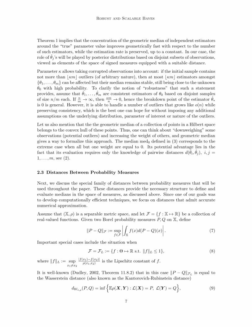
Figure 3: Effect of stochastic approximation on empirical coverage of (1-α)100% CIs. Thex-axis represents the outlier magnitude that increases from 1 to 25. The y-axisrepresents the fraction of times the CIs of M-Posteriors with and without stochas-tic approximation include the true mean over 50 replications. The horizontal lines(in violet) show the theoretical frequentist coverage.
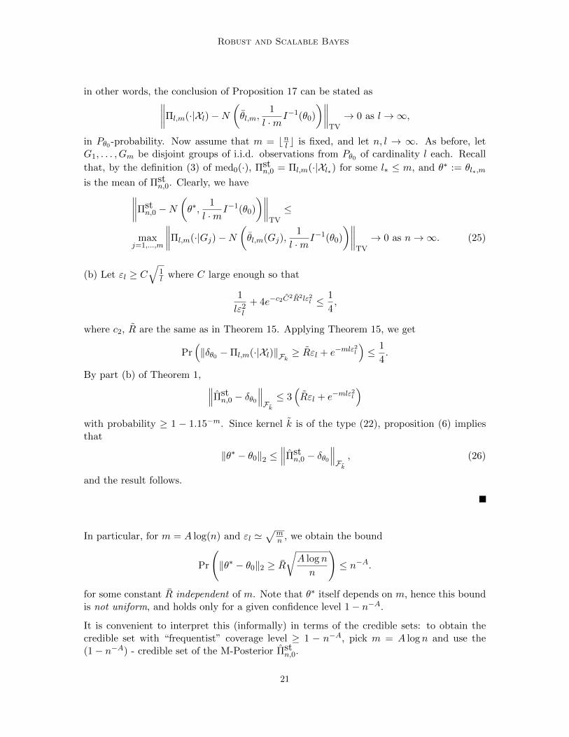
Figure 4: Effect of stochastic approximation on the length of (1-α)100% CIs. The x-axisrepresents the outlier magnitude that increases from 1 to 25. The y-axis repre-sents the differences in the lengths of the CIs of M-Posteriors without and withstochastic approximation.
fairly similar for i = 1, . . . , 25, with M-Posterior’s CIs being slightly wider in absence oflarge outliers (Figure 2).
Stochastic approximation was important for proper calibration of uncertainty quantification.The empirical coverages of (1-α)100% CIs of the M-Posterior without stochastic approxima-tion overcompensated for uncertainty at all levels of α (Figure 3). Similarly, lengths of theCIs of M-Posterior without stochastic approximation are wider than those with stochasticapproximation (Figure 4). Both these observations showed that stochastic approximationled to shorter CIs for M-Posterior that had empirical coverages close to their theoreticalvalues.
The number of subsets m had an effect on credible interval length of the M-Posterior. Wemodified the simulation above and generated 1000 observations x, with the last 10 obser-vations in x being outliers with value xj = 25 max(|x1|, . . . , |x990|), j = 991, . . . , 1000. Thesimulation setup was replicated 50 times. M-Posteriors were obtained form = 16, 18, . . . , 40, 50, 60.Across all values of m, M-Posterior’s CI was compared to the CI of the overall posterior
26
Robust and Scalable Bayes
xx
16 20 24 28 32 36 40 44 48 52 56 60
1.0
1.5
2.0
2.5
3.0
Rel
ativ
e D
iffer
ence
of M
−P
oste
rior
and
Ove
rall
Pos
terio
r C
I Len
gths
m (# subsets)
α = 0.2α = 0.15α = 0.1α = 0.05
(a) Sensitivity to the choice of m
Overall M (m = 10) M (m = 20)3.5
4.0
4.5
5.0
log 1
0 S
econ
ds
(b) Time
Figure 5: (a) Effect of m on the length of (1-α)100% CIs. The x-axis represents differentchoices of m. The y-axis represents the relative difference between M-Posteriorand overall posterior CI lengths (median across all 25 outlier magnitudes and 50replications). (b) Computation time to estimate overall posterior and M-Posterior(M) with m = 10 and m = 20 in real data analysis.
after removing the outliers; the relative difference of M-Posterior and the overall posteriorCI lengths decreases for m ≥ 22 > 2k, where k = 10 is the number of outliers, remainsstable as m increases to m = 38, and grows for larger values of m (Figure 5a). This demon-strates that inference based on M-Posterior was not too sensitive to the choice of m for awide range of values.
4.2 Real Data Analysis: General Social Survey
The General Social Survey (GSS; gss.norc.org) has collected responses to questions aboutevolution of American society since 1972. We selected data for 9 questions from differentsocial topics: “happy” (happy), “Bible is a word of God” (bible), “support capital punish-ment” (cap), “support legalization of marijuana” (grass), “support premarital sex” (pre),“approve bible prayer in public schools” (prayer), “expect US to be in world war in 10years” (uswar), “approve homosexual sex relations” (homo), “support abortion” (abort).These questions were in the survey since 1988 and their answers were converted to twolevels: yes or no. Missing data were imputed based on the average, resulting in a data setwith approximately 28,000 respondents.
We use a Dirichlet process (DP) mixture of product multinomial distributions, probabilisticparafac (p-parafac), to model the multivariate dependence among the 9 questions. Letck ∈ yes,no represent the response to kth question, k = 1, . . . , 9, then πc1,...,c9 is the jointprobability of response c = (c1, . . . , c9) for the 9 questions. Using πc1,...,c9 , we estimatedthe joint probability of response to two questions πci,cj for every i and j in 1, . . . , 9; seeSection 6 of the supplementary material for the p-parafac generative model and samplingalgorithms. The GSS data were randomly split into 10 test and training data sets. Samplesfrom the overall posteriors of πci,cj s were obtained using the Gibbs sampling algorithm ofDunson and Xing (2009). We chose m as 10 and 20 and estimated M-Posteriors for πci,cj s in
four steps: training data were randomly split into m subsets, samples from subset posteriorswere obtained after modifying the original sampler using stochastic approximation, weightsof subsets posteriors were estimated using Algorithm 2, and atoms with estimated weightsbelow 1
2m were removed.
M-Posterior had similar uncertainty quantification as the overall posterior while being moreefficient. M-Posterior was at least 10 (m = 20) and 8 times (m = 10) faster than the overallposterior and it used less than 25% of the memory resources required by the overall posterior(Figure 5b). The lengths of credible intervals for πci,cj s obtained using the overall posteriorand the two M-Posteriors were very similar, but the overall posterior’s coverage of themaximum likelihood estimators for πci,cj s obtained from the test data was worse than thatof the two M-Posteriors (Table 1).
Empirical Coverage of (1-α)100% Credible Intervals
Table 1: Empirical coverage and lengths of (1-α)100% credible intervals. The results areaveraged across all joint probabilities πci,cj s and 10 folds of cross-validation. MonteCarlo errors are in parentheses.
Acknowledgments
Authors were partially supported by grant R01-ES-017436 from the National Institute of En-vironmental Health Sciences (NIEHS) of the National Institutes of Health (NIH). StanislavMinsker acknowledges support from NSF grants DMS-1712956, FODAVA CCF-0808847,DMS-0847388, ATD-1222567. Lizhen Lin was partially supported by NSF CAREER DMS-1654579 and IIS-1663870.
28
Robust and Scalable Bayes
Appendix A. Proofs.
A.1 Proof of Theorem 1
We will prove a slightly more general result:
Theorem 20
a Assume that (H, ‖ · ‖) is a Hilbert space and θ0 ∈ H. Let θ1, . . . , θm ∈ H be a collection ofindependent random variables. Let the constants α, q, γ be such that 0 < q < α < 1/2,and 0 ≤ γ < α−q
1−q . Suppose ε > 0 is such that for all j, 1 ≤ j ≤ b(1− γ)mc+ 1,
Pr(‖θj − θ0‖ > ε
)≤ q. (28)
Let θ∗ = medg(θ1, . . . , θm) be the geometric median of θ1, . . . , θm. Then
Pr(‖θ∗ − θ0‖ > Cαε
)≤[e
(1−γ)ψ(α−γ1−γ ,q
)]−m,
where Cα = (1− α)√
11−2α .
b Assume that (Y, d) is a metric space and θ0 ∈ Y. Let θ1, . . . , θm ∈ Y be a collectionof independent random variables. Let the constants q, γ be such that 0 < q < 1
2 and
0 ≤ γ < 1/2−q1−q . Suppose ε > 0 are such that for all j, 1 ≤ j ≤ b(1− γ)mc+ 1,
Pr(d(θj , θ0) > ε
)≤ q. (29)
Let θ∗ = med0(θ1, . . . , θm). Then
Pr(d(θ∗, θ0) > 3ε
)≤ e−m(1−γ)ψ
(1/2−γ1−γ ,q
).
To get the bound stated in the paper, take q = 17 and α = 3
7 in part (a) and q = 14 in part
b.
We start by proving part a. To this end, we will need the following lemma (see lemma 2.1in Minsker, 2015):
Lemma 21 Let H be a Hilbert space, x1, . . . , xm ∈ H and let x∗ be their geometric median.Fix α ∈
(0, 1
2
)and assume that z ∈ H is such that ‖x∗ − z‖ > Cαr, where
Cα = (1− α)
√1
1− 2α
and r > 0. Then there exists a subset J ⊆ 1, . . . ,m of cardinality |J | > αm such that forall j ∈ J , ‖xj − z‖ > r.
29
Minsker et al.
Assume that event E :=‖θ∗ − θ0‖ > Cαε
occurs. Lemma 21 implies that there exists a
subset J ⊆ 1, . . . ,m of cardinality |J | ≥ αk such that ‖θj − θ0‖ > ε for all j ∈ J , hence
Pr(E) ≤Pr
m∑j=1
I‖θj − θ0‖ > ε
> αm
≤Pr
b(1−γ)mc+1∑j=1
I‖θj − θ0‖ > ε
> (α− γ)m
b(1− γ)mc+ 1
b(1− γ)mc+ 1
≤Pr
b(1−γ)mc+1∑j=1
I‖θj − θ0‖ > ε
>α− γ1− γ
(b(1− γ)mc+ 1
) .
If W has Binomial distribution W ∼ B(b(1− γ)mc+ 1, q), then
Pr
( b(1−γ)mc+1∑j=1
I‖θj − θ0‖ > ε
>α− γ1− γ
(b(1− γ)mc+ 1
))≤
Pr
(W >
α− γ1− γ
(b(1− γ)mc+ 1
))(see Lemma 23 in Lerasle and Oliveira, 2011 for a rigorous proof of this fact). Chernoffbound (e.g., Proposition A.6.1 in van der Vaart and Wellner, 1996), together with an obviousbound b(1− γ)mc+ 1 > (1− γ)m, implies that
Pr
(W >
α− γ1− γ
(b(1− γ)mc+ 1
))≤ exp
(−m(1− γ)ψ
(α− γ1− γ
, q
)).
To establish part b, we proceed as follows: let E1 be the event
E1 = more than a half of events d(θj , θ0) ≤ ε, j = 1 . . .m occur.
Assume that E1 occurs. Then we clearly have ε∗ ≤ ε, where ε∗ is defined in equation (2.2)of the paper: indeed, for any θj1 , θj2 such that d(θji , θ0) ≤ ε, i = 1, 2, triangle inequality
gives d(θj1 , θj2) ≤ 2ε. By the definition of θ∗, inequality d(θ∗, θj) ≤ 2ε∗ ≤ 2ε holds for at
least a half of θ1, . . . , θm, hence, it holds for some θj with d(θj , θ0) ≤ ε. In turn, this
implies (by triangle inequality) d(θ∗, θ0) ≤ 3ε. We conclude that
Pr(d(θ∗, θ0) > 3ε
)≤ Pr(E1).
The rest of the proof repeats the argument of part a since
Pr(Ec1) = Pr
m∑j=1
Id(θj , θ0) > ε
≥ m
2
,
where Ec1 is the complement of E1.
30
Robust and Scalable Bayes
A.2 Proof of Theorem 7
By the definition of Wasserstein distance dW1 ,
dW1,ρ(δ0,Πl(·|Xl)) =
∫Θρ(θ, θ0)dΠl(θ|X1, . . . , Xl). (30)
(recall that ρ is the Hellinger distance). Let R be a large enough constant to be determinedlater. Note that the Hellinger distance is uniformly bounded by 1. Using (30), it is easy tosee that
dW1,ρ(δ0,Πl(·|Xl)) ≤ Rεl +
∫ρ(θ,θ0)≥Rεl
dΠl(·|Xl). (31)
To this end, it remains to estimate the second term in the sum above. We will follow theproof of Theorem 2.1 in Ghosal et al. (2000). Bayes formula implies that
Πl(θ : ρ(θ, θ0) ≥ Rεl|Xl) =
∫ρ(θ,θ0)≥Rεl
∏li=1
pθp0
(Xi)dΠ(θ)∫Θ
∏li=1
pθp0
(Xi)dΠ(θ).
Let
Al =
θ : −P0
(log
pθp0
)≤ ε2
l , P0
(log
pθp0
)2
≤ ε2l
.
For any C1 > 0, Lemma 8.1 Ghosal et al. (2000) yields
Pr
∫Θ
l∏i=1
pθp0
(Xi)dQ(θ) ≤ exp(− (1 + C1)lε2
l
) ≤ 1
C21 lε
2l
.
for every probability measure Q on the set Al. Moreover, by the assumption on the priorΠ,
Π(Al) ≥ exp(−Clε2
l
).
Consequently, with probability at least 1− 1C2
1 lε2l,
∫Θ
l∏i=1
pθp0
(Xi)dΠ(θ) ≥ exp(− (1 + C1)lε2
l
)Π(Al) ≥ exp(−(1 + C1 + C)lε2
l ).
Define the event Bl =
∫Θ
l∏i=1
pθp0
(Xi)dΠ(θ) ≤ exp(− (1 + C1 + C)lε2
l
).
Let Θl be the set satisfying conditions of Theorem 3.1. Then by Theorem 7.1 in Ghosalet al. (2000), there exist test functions φl := φl(X1, . . . , Xl) and a universal constant Ksuch that
To estimate the second term of last equation, note that
EP0
∫ρ(θ,θ0)≥Rεl
l∏i=1
pθp0
(Xi)dΠ(θ)(1− φl) ≤
EP0
( ∫θ∈Θ\Θl
l∏i=1
pθp0
(Xi)dΠ(θ)(1− φl) +
∫Θl∩ρ(θ,θ0)≥Rεl
l∏i=1
pθp0
(Xi)dΠ(θ)(1− φl)
)≤
Π(Θ\Θl) +
∫Θl∩ρ(θ,θ0)≥Rεl
EP0
(l∏
i=1
pθp0
(Xi)dΠ(θ)(1− φl)
)≤ (35)
e−lε2l (C+4) + e−KR
2·lε2l ≤ 2e−lε2l (C+4)
for R ≥√
(C + 4)/K. Set C1 = 1 and note that IBl = 1 with probability P (Bl) ≤ 1/lε2l .
It follows from (33), (34) and (35) and Chebyshev’s inequality that for any t > 0
Pr(
Πl(θ : ρ(θ, θ0) ≥ Rεl|Xl) ≥ t)≤ Pr(Bl) +
2e−Klε2l
t+
2 exp(−2lε2
l
)t
≤ 1
lε2l
+2e−Klε
2l
t+
2 exp(−2lε2
l
)t
.
Finally, for a constant K = min(K/2, 1) and t = e−Klε2l , we obtain
Pr(
Πl(θ : ρ(θ, θ0) ≥ Rεl|Xl) ≥ t)≤ 1
lε2l
+ 2e−Klε2l /2 + 2 exp
(−lε2
l
)≤ 1
lε2l
+ 4e−Klε2l ,
which yields the result.
32
Robust and Scalable Bayes
A.3 Proof of Theorem 12
From equation (20) in the paper and proceeding as in proof of Theorem 7, we get that
‖δ0 −Πl(·|Xl)‖Fk ≤ Rε1/γl +
∫ρk(θ,θ0)≥Rε1/γl
ρk(θ, θ0)dΠl(·|Xl).
By Holder’s inequality,∫ρk(θ,θ0)≥Rε1/γl
ρk(θ, θ0)dΠl(·|Xl) ≤
∫Θ
ρwk (θ, θ0)dΠl(·|Xl)
1/w ∫ρk(θ,θ0)≥Rε1/γl
dΠl(·|Xl)
1/q
with w > 1 and q = ww−1 .
Define the event
Bl =
∫Θ
l∏i=1
pθp0
(Xi)dΠ(θ) ≥ exp(− (1 + C1 + C)lε2
l
) .
Following in the proof of Theorem 3.1, we note that Pr(Bl) ≥ 1 − 1C2
1 lε2l
(where constants
C,C1 are the same as in the proof of Theorem 7). Also, note that
EP0
[∫Θρwk (θ, θ0)
l∏i=1
pθp0
(Xi)dΠ(θ)
]=
∫Θρwk (θ, θ0)dΠ(θ)
Hence, with probability ≥ 1− e−Klε2l ,∫Θρwk (θ, θ0)
l∏i=1
pθp0
(Xi)dΠ(θ) ≤ eKlε2l∫
Θρwk (θ, θ0)dΠ(θ),
where K = min(K/2, 1) is the same universal constant as in the proof of Theorem 7. Writing∫Θ
ρwk (θ, θ0)dΠl(·|Xl)
1/w
=
[∫Θ ρ
wk (θ, θ0)
∏li=1
pθp0
(Xi)dΠ(θ)∫Θ
∏li=1
pθp0
(Xi)dΠ(θ)
]1/w
,
we deduce that with probability ≥ 1− e−Klε2l − 1lε2l
(where we set C1 := 1),∫Θ
ρwk (θ, θ0)dΠl(·|Xl)
1/w
≤ e2+C+K
wlε2l
[∫Θρwk (θ, θ0)dΠ(θ)
]1/w
.
33
Minsker et al.
By Theorem 7.1 in Ghosal et al. (2000), there exist test functions φl := φl(X1, . . . , Xl) anda universal constant K such that
EP0φl ≤ 2e−Klε2l ,
supθ∈Θl,d(θ,θ0)≥Rεl
EPθ(1− φl) ≤ e−KR2·lε2l ,
where KR2−1 > K and d(·, ·) is the Hellinger or Euclidean distance. It immediately followsfrom Assumption 3.4 that
θ : ρ(θ, θ0) ≥ C0(θ0)Rγεl
⊇θ : ρk(θ, θ0) ≥ Rε1/γ
l
,
hence the test functions φl (for R := C0(θ0)Rγ) satisfy
EP0φl ≤ 2e−Klε2l , (36)
supθ∈Θl,ρk(θ,θ0)≥Rε1/γl
EPθ(1− φl) ≤ e−KR2·lε2l .
Repeating the steps of the proof of Theorem 7, we see that if R is chosen large enough, then∫ρk(θ,θ0)≥Rε1/γl
dΠl(·|Xl) ≤ e−Klε2l
with probability ≥ 1 − 1lε2l− 4e−Klε
2l . Combining the bounds, we obtain that, for w :=
43 + 4+2C
3K, with probability ≥ 1− 1
lε2l− 5e−Klε
2l ,∫
ρ(θ,θ0)≥Rε1/γl
ρk(θ, θ0)dΠl(·|Xl) ≤ e−Klε2l /2
[∫Θρwk (θ, θ0)dΠ(θ)
]1/w
,
hence the result follows.
A.4 Proof of Theorem 15
The proof strategy is similar to Theorem 7. Note that
dW1,ρ(δ0,Πn,m(·|Xl)) ≤ Rεl +
∫h(Pθ,P0)≥Rεl
dΠl(·|Xl), (37)
where h(·, ·) is the Hellinger distance.
Let El := θ : h(Pθ, P0) ≥ Rεl. By the definition of Πn,m, we have
Πn,m(El|Xl) =
∫El
(∏lj=1
pθp0
(Xj))m
dΠ(θ)∫Θ
(∏lj=1
pθp0
(Xj))m
dΠ(θ). (38)
34
Robust and Scalable Bayes
To bound the denominator from below, we proceed as before. Let
Θl =
θ : −P0
(log
pθp0
)≤ ε2
l , P0
(log
pθp0
)2
≤ ε2l
.
Let Bl be the event defined by
Bl :=
∫Θl
(l∏
i=1
pθp0
(Xi)
)mdQ(θ) ≤ exp(−2mlε2
l )
,
where Q is a probability measure supported on Θl. Lemma 8.1 in Ghosal et al. (2000)yields that Pr(Bl) ≤ 1
lε2lfor any Q, in particular, for the conditional distribution Π(·|Θl).
We conclude that∫Θ
l∏j=1
pθp0
(Xj)
m
dΠ(θ) ≥ Π(Θl) exp(−2mlε2l ) ≥ exp(−(2m+ C)lε2
l ).
To estimate the numerator in (38), note that if Theorem 3.10 holds for γ = εl, then it alsoholds for γ = Lεl for any L ≥ 1. This observation implies that
supθ∈El
l∏j=1
pθp0
(Xj)
m
≤ e−c1R2mlε2l
with probability ≥ 1− 4e−c2R2lε2l , hence
∫El
l∏j=1
pθp0
(Xj)
m
dΠ(θ) ≤ e−c1R2mlε2l
with the same probability. Choose R = R(C) large enough so that c1mR2 ≥ 3m + C.
Putting the bounds for the numerator and denominator of (38) together, we get that withprobability ≥ 1− 1
lε2l− 4e−c2R
2lε2l ,
Πn,m(El|Xl) ≤ e−mlε2l .
The result now follows from (37).
A.5 Proof of Proposition 17
The proof follows a standard pattern: on the first step, we show that it is enough to considerthe posterior obtained from the prior restricted to a large compact set, and then provingthe theorem for the prior with compact support. The second part mimics the classicalargument exactly (e.g., see van der Vaart, 2000).
35
Minsker et al.
To show that one can restrict the prior to the compact set, it is enough to establish thatfor R large enough and El := θ : ‖θ − θ0‖ ≥ R√
l,
Πn,m(El|Xl) =
∫El
(∏lj=1
pθp0
(Xj))m
dΠ(θ)∫Θ
(∏lj=1
pθp0
(Xj))m
dΠ(θ)(39)
can be made arbitrarily small. This follows from the inclusion
El ⊆θ : h(Pθ, Pθ0) ≥ C R√
l
(due to the assumed inequality between Hellinger and Euclidean distances) and the boundsfor the numerator and the denominator of (39) established in the proof of Theorem 15.
A.6 Selection of the optimal number of subsets m
The following heuristic approach picks the median among the candidate M -posteriors.Namely, start by evaluating the M-Posterior for each m in the range of candidate values[m1,m2]:
Πgn,m1 := medg(Π
(1)n , . . . ,Π
(m1)n ),
Πgn,m1+1 := medg(Π
(1)n , . . . ,Π
(m1+1)n ),
...
Πgn,m2 := medg(Π
(1)n , . . . ,Π
(m2)n )
and choose m∗ ∈ [m1,m2] such that
Πgn,m∗ = med0
(Πgn,m1
, Πgn,m1+1, . . . , Π
gn,m2
), (40)
where med0 is the metric median defined in (3) in Section 2.2.
References
Alekh Agarwal and John C Duchi. Distributed delayed stochastic optimization. In 2012IEEE 51st Annual Conference on Decision and Control (CDC), pages 5451–5452, 2012.
Sungjin Ahn, Anoop Korattikara, and Max Welling. Bayesian posterior sampling viastochastic gradient Fisher scoring. Proceedings of the 29th International Conference onMachine Learning (ICML-12), 2012.
Noga Alon, Yossi Matias, and Mario Szegedy. The space complexity of approximatingthe frequency moments. In Proceedings of the twenty-eighth annual ACM symposium onTheory of computing, pages 20–29. ACM, 1996.
Nachman Aronszajn. Theory of reproducing kernels. Transactions of the American math-ematical society, 68(3):337–404, 1950.
(b) Expect US to be in world war in 10 years (uswar) and support abortion (abort)
Figure 6: Kernel density estimators of subset posteriors (dashed), M-Posterior with m = 10(blue) and m = 20 (violet), and the overall posterior (red) for the four responses.In particular, the model “recognizes” that “expect US to be in world war in 10years” (uswar) and “support abortion” (abort) should be independent.
M. J. Bayarri and James O. Berger. Robust Bayesian bounds for outlier detection. RecentAdvances in Statistics and Probability, pages 175–190, 1994.
Amir Beck and Shoham Sabach. Weiszfeld’s method: old and new results. Preprint,2013. Available at https://iew3.technion.ac.il/Home/Users/becka/Weiszfeld_
review-v3.pdf.
James O. Berger. An overview of robust Bayesian analysis. Test, 3(1):5–124, 1994.
Christopher M. Bishop. Pattern Recognition and Machine Learning. Springer, New York,2006.
Emmanuel Boissard and Thibaut Le Gouic. On the mean speed of convergence of empiricaland occupation measures in wasserstein distance. Ann. Inst. H. Poincare Probab. Statist.,50(2):539–563, 2014.
Prosenjit Bose, Anil Maheshwari, and Pat Morin. Fast approximations for sums of distances,clustering, and the Fermat–Weber problem. Computational Geometry, 24(3):135–146,2003.
George EP Box and George C Tiao. A Bayesian approach to some outlier problems.Biometrika, 55(1):119–129, 1968.
Stephen Boyd, Neal Parikh, Eric Chu, Borja Peleato, and Jonathan Eckstein. Distributedoptimization and statistical learning via the alternating direction method of multipliers.Foundations and Trends in Machine Learning, 3(1):1–122, 2011.
Tamara Broderick, Nicholas Boyd, Andre Wibisono, Ashia C Wilson, and Michael Jordan.Streaming variational Bayes. In Advances in Neural Information Processing Systems,pages 1727–1735, 2013.
Herve Cardot, Peggy Cenac, and Pierre-Andre Zitt. Recursive estimation of the conditionalgeometric median in Hilbert spaces. Electronic Journal of Statistics, 6:2535–2562, 2012.
Herve Cardot, Peggy Cenac, and Pierre-Andre Zitt. Efficient and fast estimation of thegeometric median in Hilbert spaces with an averaged stochastic gradient algorithm.Bernoulli, 19(1):18–43, 2013.
Bob Carpenter, Andrew Gelman, Matt Hoffman, Daniel Lee, Ben Goodrich, Michael Be-tancourt, Michael A Brubaker, Jiqiang Guo, Peter Li, and Allen Riddell. Stan: A prob-abilistic programming language. Journal of Statistical Software, 20:1–37, 2016.
Ramaswamy Chandrasekaran and Arie Tamir. Algebraic optimization: the Fermat-Weberlocation problem. Mathematical Programming, 46(1-3):219–224, 1990.
Kjell A Doksum and Albert Y Lo. Consistent and robust Bayes procedures for locationbased on partial information. The Annals of Statistics, pages 443–453, 1990.
Richard M Dudley. Real Analysis and Probability, volume 74. Cambridge University Press,2002.
David B Dunson and Chuanhua Xing. Nonparametric Bayes modeling of multivariatecategorical data. Journal of the American Statistical Association, 104(487):1042–1051,2009.
Nicolas Fournier and Arnaud Guillin. On the rate of convergence in wasserstein distance ofthe empirical measure. Probability Theory and Related Fields, 162(3):707–738, Aug 2015.
Subhashis Ghosal, Jayanta K Ghosh, and Aad W Van Der Vaart. Convergence rates ofposterior distributions. Annals of Statistics, 28(2):500–531, 2000.
Peter D Hoff. Extending the rank likelihood for semiparametric copula estimation. TheAnnals of Applied Statistics, pages 265–283, 2007.
38
Robust and Scalable Bayes
Matthew D. Hoffman, David M. Blei, Chong Wang, and John Paisley. Stochastic variationalinference. Journal of Machine Learning Research, 14:1303–1347, 2013.
Giles Hooker and Anand N Vidyashankar. Bayesian model robustness via disparities. Test,23(3):556–584, 2014.
Daniel Hsu and Sivan Sabato. Loss minimization and parameter estimation with heavytails. arXiv preprint arXiv:1307.1827, 2013.
Peter J. Huber and Elvezio M. Ronchetti. Robust Statistics. Wiley Series in Probabilityand Statistics. John Wiley & Sons Inc., second edition, 2009.
J. H. B. Kemperman. The median of a finite measure on a Banach space. Statistical DataAnalysis Based on the L1-norm and Related Methods, North-Holland, Amesterdam, pages217–230, 1987.
Ariel Kleiner, Ameet Talwalkar, Purnamrita Sarkar, and Michael I Jordan. A scalablebootstrap for massive data. Journal of the Royal Statistical Society: Series B (StatisticalMethodology), 76(4):795–816, 2014.
Anoop Korattikara, Yutian Chen, and Max Welling. Austerity in MCMC land: cutting theMetropolis-Hastings budget. arXiv preprint arXiv:1304.5299, 2013.
Matthieu Lerasle and Roberto I. Oliveira. Robust empirical mean estimators. arXiv preprintarXiv:1112.3914, 2011.
Hendrik P Lopuhaa and Peter J Rousseeuw. Breakdown points of affine equivariant esti-mators of multivariate location and covariance matrices. The Annals of Statistics, pages229–248, 1991.
Jeffrey W Miller and David B Dunson. Robust Bayesian inference via coarsening. arXivpreprint arXiv:1506.06101, 2015.
Stanislav Minsker. Geometric median and robust estimation in Banach spaces. Bernoulli,21(4):2308–2335, 2015.
Willie Neiswanger, Chong Wang, and Eric Xing. Asymptotically exact, embarrassinglyparallel MCMC. arXiv preprint arXiv:1311.4780, 2013.
Arkadi S. Nemirovskiı and B. Yudin David. Problem Complexity and Method Efficiency inOptimization. A Wiley-Interscience publication. Wiley, 1983.
Frank Nielsen and Vincent Garcia. Statistical exponential families: a digest with flashcards. arXiv preprint arXiv:0911.4863, 2011.
Lawrence M. Ostresh. On the convergence of a class of iterative methods for solving theWeber location problem. Operations Research, 26(4):597–609, 1978.
Michael L. Overton. A quadratically convergent method for minimizing a sum of Euclideannorms. Mathematical Programming, 27(1):34–63, 1983.
Carl Edward Rasmussen and Christopher KI Williams. Gaussian processes for machinelearning. the MIT Press, 2, 2006.
39
Minsker et al.
Steven L Scott, Alexander W Blocker, Fernando V Bonassi, Hugh A Chipman, Edward IGeorge, and Robert E McCulloch. Bayes and big data: the consensus Monte Carloalgorithm, 2013.
Alexander Smola and Shravan Narayanamurthy. An Architecture for Parallel Topic Models.In Very Large Databases (VLDB), 2010.
Bharath K Sriperumbudur, Kenji Fukumizu, Arthur Gretton, Bernhard Scholkopf, andGert RG Lanckriet. On integral probability metrics, φ-divergences and binary classifica-tion. arXiv:0901.2698, 2009.
Bharath K Sriperumbudur, Arthur Gretton, Kenji Fukumizu, Bernhard Scholkopf, andGert RG Lanckriet. Hilbert space embeddings and metrics on probability measures. TheJournal of Machine Learning Research, 99:1517–1561, 2010.
Sanvesh Srivastava, Volkan Cevher, Quoc Dinh, and David Dunson. WASP: Scalable Bayesvia barycenters of subset posteriors. In Proceedings of the 18th International Conferenceon Artificial Intelligence and Statistics, pages 912–920, 2015a.
Sanvesh Srivastava, Cheng Li, and David B Dunson. Scalable Bayes via barycenter inWasserstein space. arXiv preprint arXiv:1508.05880, 2015b.
Markus Svensen and Christopher M Bishop. Robust Bayesian mixture modelling. Neuro-computing, 64:235–252, 2005.
Aad van der Vaart. Asymptotic Statistics. Cambridge university press, 2000.
Aad van der Vaart and Jon A. Wellner. Weak Convergence and Empirical Processes.Springer Series in Statistics. Springer-Verlag, New York, 1996.
Chong Wang, John W Paisley, and David M Blei. Online variational inference for thehierarchical Dirichlet process. In International Conference on Artificial Intelligence andStatistics, pages 752–760, 2011.
Xiangyu Wang and David B Dunson. Parallel MCMC via Weierstrass sampler. arXivpreprint arXiv:1312.4605, 2013.
Endre Weiszfeld. Sur un probleme de minimum dans l’espace. Tohoku Mathematical Journal,1936.
Max Welling and Yee W Teh. Bayesian learning via stochastic gradient Langevin dynamics.In Proceedings of the 28th International Conference on Machine Learning (ICML-11),pages 681–688, 2011.
Wing Hung Wong, Xiaotong Shen, et al. Probability inequalities for likelihood ratios andconvergence rates of sieve MLEs. The Annals of Statistics, 23(2):339–362, 1995.