Robust Beamforming Design in C-RAN withSigmoidal Utility and Capacity-Limited Backhaul

Zehua Wang, Member, IEEE, Derrick Wing Kwan Ng, Member, IEEE,Vincent W.S. Wong, Fellow, IEEE, and Robert Schober, Fellow, IEEE

Abstract—In the paper, we study the robust beamformingdesign in cloud radio access networks where remote radio heads(RRHs) are connected to a cloud server that performs signalprocessing and resource allocation in a centralized manner. Dif-ferent from traditional approaches adopting a concave increasingfunction to model the utility of a user, we model the utilityby a sigmoidal function of the signal-to-interference-plus-noiseratio (SINR) to capture the diminishing utility returns for verysmall and very large SINRs in real-time applications (e.g. videostreaming). Our objective is to maximize the aggregate utility ofthe users while taking into account the imperfection of channelstate information (CSI), limited backhaul capacity, and minimumquality of service requirements. Because of the sigmoidal utilityfunction and some of the constraints, the formulated problemis non-convex. To efficiently solve the problem, we introduce amaximum interference constraint, transform the CSI uncertaintyconstraints into linear matrix inequalities, employ convex relax-ation to handle the backhaul capacity constraints, and exploitthe sum-of-ratios form of the objective function. This leads to anefficient resource allocation algorithm which outperforms severalbaseline schemes and closely approaches a performance upperbound for large CSI uncertainty or large number of RRHs.

Index Terms: C-RAN, beamforming design, imperfect CSI, sig-moidal utility function, capacity-limited backhaul.

I. INTRODUCTION

Deploying base stations (BSs) densely is a viable approachto meet the tremendous data traffic demands in the fifth gen-eration (5G) wireless communication networks [2]. However,this may also increase the capital and operational expenditureof mobile network operators (MNOs) and the user equipments(UEs) may suffer from severe multicell interference caused bysimultaneous transmissions in adjacent cells [3]. The recentlyproposed cloud radio access network (C-RAN) architecture is

Manuscript received September 26, 2016; revised April 3, 2017; acceptedMay 23, 2017. This work was supported by the Natural Sciences andEngineering Research Council of Canada (NSERC). Part of this paper waspresented at the IEEE International Conference on Communications (ICC),Kuala Lumpur, Malaysia, May 2016 [1]. The review of this paper wascoordinated by Prof. Pierluigi Salvo Rossi.

Zehua Wang and Vincent W.S. Wong are with the Department of Electricaland Computer Engineering, The University of British Columbia, Vancouver,BC, V6T 1Z4, Canada (e-mail: zwang@ece.ubc.ca; vincentw@ece.ubc.ca).

Derrick Wing Kwan Ng is with School of Electrical Engineering andTelecommunications, The University of New South Wales, Sydney, Aus-tralia (email: w.k.ng@unsw.edu.au). He is supported under Australian Re-search Council’s Discovery Early Career Researcher Award funding scheme(DE170100137).

Robert Schober is with the Institute for Digital Communications,Friedrich-Alexander University of Erlangen–Nuremberg, Germany (email:robert.schober@fau.de)

Color versions of one or more of the figures in this paper are availableonline at http://ieeexplore.ieee.org.

Digital Object Identifier 10.1109/TWC.2017.XXXXXXX

considered to be a promising architecture to overcome theseproblems in 5G wireless networks [4]. In C-RAN, the radiosignal transceiver module and the baseband signal processingmodule of conventional BSs are detached. The baseband signalprocessing module is located at a cloud server and is referredto as baseband unit (BBU). The BS, which is only composedof radio signal transceivers in C-RAN, is referred to as re-mote radio head (RRH). Ideally, the backhaul communicationbetween the RRHs and the BBUs is implemented by opticalfibers. Multiple BBUs running on a cloud server can forma computationally powerful BBU pool, where the basebandsignals are processed in a centralized manner. Thus, not onlythe cost of deploying a new BS can be significantly reduced,but also coordinated multipoint (CoMP) transmission can beseamlessly applied to mitigate the interference caused bynearby BSs.

Due to these advantages inherent to C-RAN, coordinatedbeamforming design has been studied for C-RAN in theliterature [5]–[9] to improve system performance. The authorsin [5] formulated an optimization problem for the beamform-ing design in CoMP networks with the objective of minimizingthe backhaul data traffic. Beamforming design for reducing theenergy consumption and increasing the energy efficiency of C-RAN was studied in [6]–[8] for various network scenarios. Thework in [6] assumed imperfect channel state information (CSI)for beamforming design for downlink data transmission. Thework in [7] investigated beamforming design for both uplinkand downlink for minimization of the energy consumptionin C-RAN. Maximizing the energy efficiency via cooperativebeamforming was proposed in [8]. The authors in [9] formu-lated a multi-objective optimization problem to jointly reducethe backhaul data traffic and the energy consumption of theRRHs. However, it was assumed in [6]–[9] that an unlimitedamount of control signals, user CSI, and precoding data canbe exchanged over the backhaul.

In practice, the backhaul capacity is limited. Taking thisconstraint into account for beamforming design is crucial inC-RAN. In the literature, there are two strategies to limitthe amount of backhaul data traffic in C-RAN, namely, thecompression strategy and the data sharing strategy [10]. Forthe compression strategy, the backhaul data traffic is reducedby adopting source coding techniques. Specifically, the res-olution of the compressed signals is adjusted according tothe backhaul capacity. The compression strategy has beeninvestigated for both uplink and downlink transmission in C-RAN. In particular, the authors of [11] and [12] assumed thatthe quantization noises at different RRHs are uncorrelated and

used independent compression for uplink data transmission.By exploiting the correlation of the quantization noises atdifferent RRHs, distributed compression schemes have beenproposed for uplink data transmission in [13]–[18]. On the oth-er hand, the authors of [19] studied downlink data transmissionemploying independent compression. Independent compres-sion for downlink data transmission with imperfect CSI wasstudied in [20]. Furthermore, the authors of [21] investigateddistributed compression for downlink data transmission in C-RAN. However, different mobile applications running on theUEs may require different resolutions for the received signals,which increases the complexity of the baseband signal pro-cessing if the compression strategy is employed. For the datasharing strategy, the amount of backhaul data traffic of an RRHis determined by the data traffic of the UEs that are associatedwith the RRH. The association problem between UEs andRRHs can be solved either by a clustering approach [22]or a user-centric approach [10]. The former approach allowsmultiple RRHs to form a cluster for serving multiple UEs.However, geographic boundaries exist between adjacent RRHclusters. The UEs located at the boundaries of RRH clustersmay suffer from strong co-channel interference. The latterapproach, in contrast, dynamically selects suitable RRHs toserve individual UE by exploiting the benefits of interferencemanagement. In fact, the user-centric approach can effectivelyreduce the co-channel interference by associating each UE tomultiple RRHs and employing an appropriate beamformingdesign. Thus, different from [19]–[21], in this paper, we adoptthe data sharing strategy and use the user-centric approach forthe association of UEs and RRHs.

Mobile applications running on UEs require differentamounts of network resources to achieve the desired qualityof service (QoS). For example, the signal-to-interference-plus-noise ratios (SINRs) needed for online video and audio stream-ing applications to ensure smooth video and audio services aredifferent. With the C-RAN architecture, the MNO can allocatethe limited network resources efficiently via cooperative beam-forming. Although many existing works [23], [24] target themaximization of the system sum rate characterized by a sumof concave increasing functions of the SINRs, sigmoidal func-tions with the received SINR as the input parameter constitutebetter models for the utility achieved by mobile users [25],[26]. However, sigmoidal functions are non-convex and thusdetermining the optimal beamforming vectors is a challengingtask. Furthermore, due to the channel noise, interference, andtime varying nature of wireless channels, only imperfect CSIcan be obtained and exploited for beamforming design inpractice. Note that the baseband signal processing in C-RANis performed by the BBU pool on a cloud server. Thus, theCSI estimated by the RRHs needs to be first conveyed to thecloud server via the capacity-limited backhaul links. Then,the precoded signals are transmitted from the BBU pool tothe RRHs. The resulting round trip delay in the backhauland the associated signal processing delay further add to theimperfection of the estimated CSI used for resource allocation.If the actual link quality between the RRHs and a UE is worsethan the estimated value, then the UE may not be able todecode the signal received from the RRHs. In this case, the

utility of the serving UE may be significantly reduced.

To address above issues, in this paper, we focus on theutility based beamforming design in C-RAN where we takeinto account both the imperfection of the CSI and the capacity-limited backhaul. To the best of our knowledge, beamformingdesign for aggregate utility maximization of mobile users in C-RAN with imperfect CSI and capacity-limited backhaul linkshas not yet been studied in the existing literature [5]–[10],[18], [21], [22]. We first formulate the robust beamformingdesign as an optimization problem. The problem is generallyintractable since it has a non-convex objective function, non-convex combinatorial constraints due to the limited backhaulcapacity, and infinitely many constraints due to the channeluncertainty. To strike a balance between system performanceand the computational complexity of solving the problem, wefocus on the design of a computationally efficient resourceallocation algorithm. In particular, we first introduce an addi-tional robust maximum interference constraint for each mobileuser to simplify the considered problem. Subsequently, wetransform the infinitely many constraints in our problem to afinite number of linear matrix inequality (LMI) constraints. Wethen adopt the convex relaxation technique to handle the non-convex combinatorial constraints, such that the transformedproblem can be solved in an iterative manner. In each iteration,we introduce an inner loop that exploits the sum-of-ratios formof the objective function to decompose the problem into twosubproblems and tackles them with semidefinite programming(SDP) and the damped Newton’s method iteratively. Simula-tion results show that the beamforming design obtained withour proposed algorithm can increase the aggregate utility inC-RAN compared with existing beamforming designs thateither maximize the weighted system sum rate (WSSR) orthe weighted sum of SINRs of the users.

The remainder of this paper is organized as follows. InSection II, we introduce the system model and present theproblem formulation. In Section III, we transform our problemand propose an iterative algorithm to obtain an efficient subop-timal solution. Simulation results are provided in Section IV.Conclusions are drawn in Section V.

Notations: In this paper, the following notations are adopted:XT, XH, Tr(X), and Rank(X) represent the transpose, con-jugate transpose, trace, and rank of matrix X, respectively;C is the set of complex numbers, Cm×n represents the setof m × n complex matrices, Hn denotes the set of n × nHermitian matrices; | · | is the absolute value. ∥ · ∥x is theℓx-norm. In particular, ∥·∥0 is the ℓ0-norm of a vector anddenotes the number of non-zero entries in the vector; E [·]denotes statistical expectation, ℜx denotes the real part ofcomplex number x; x ≽ 0 means that each element in vectorx is non-negative, X ≽ 0 (or X ≻ 0) means that matrix Xis positive semidefinite (or positive definite), x[m:n] returns avector containing the mth to the nth elements of vector x; Inis the n×n identity matrix, On is the n×n all-zero matrix, 0n

denotes the n× 1 all-zero vector; ⊗ stands for the Kroneckerproduct, and CN (0, σ2) is the zero-mean complex Gaussiandistribution with varianceσ2.

UE

RRH

optical fiber

1

3

24

56

C1

C2

C3

C4 C5 C6

BBU pool

Fig. 1. An example of a C-RAN, where four UEs are served by six RRHsvia cooperative beamforming. A BBU pool is hosted by a cloud server. TheRRHs communicate with the BBU pool on the cloud server over backhaullinks implemented by optical fibers having limited capacities denoted byC1, C2, . . . , C6. The MNO can control the RRHs and allocate networkresources to UEs in a centralized manner.

II. SYSTEM MODEL AND PROBLEM FORMULATION

We now present our system model and formulate the prob-lem. We consider downlink data transmission in a C-RAN. Anexample of the considered system is shown in Fig. 1.

A. System Model

Let M = 1, . . . ,M denote the set of RRHs in the C-RAN. Each RRH is equipped with N ≥ 1 antennas. Weassume that each mobile user has one UE. Therefore, in thesequel, we use the terms “mobile user” and “UE” interchange-ably. Let K= 1, . . . ,K denote the set of UEs. We assumethat each UE in set K is equipped with a single antenna tolimit the receiver complexity.. As beamforming and CoMPare employed, a UE can be associated with multiple RRHssimultaneously. The precoded signal transmitted from RRHm∈M to UE k∈K is given by wm,ksk, where wm,k ∈ CN×1

is the beamforming vector for UE k employed by RRH m andsk ∈ C denotes the data symbol for UE k. Without loss ofgenerality, we assume that E

[|sk|2

]= 1, ∀ k ∈ K. We note

that when wm,k = 0N , UE k is associated with RRH m.Otherwise, wm,k = 0N holds. Therefore, the signal receivedat UE k ∈ K can be written as∑

m∈MhHm,kwm,ksk︸ ︷︷ ︸

desired signal

+∑

u∈K\k

∑m∈M

hHm,kwm,usu︸ ︷︷ ︸

interfering signals

+nk,

(1)

where hm,k∈CN×1 denotes the instantaneous channel vectorfrom RRH m to UE k and nk∼CN (0, σ2

k) denotes the noiseat UE k with power σ2

k. The received SINR at UE k is givenby

γk =

∣∣∣∑m∈M hHm,kwm,k

∣∣∣2∑u∈K\k

∣∣∣∑m∈M hHm,kwm,u

∣∣∣2 + σ2k

. (2)

Due to the non-negligible round-trip delay in the backhauland the imperfection of CSI estimation, the actual CSI, hm,k,from RRH m ∈ M to UE k ∈ K in (1) may deviatefrom the estimated CSI used by the BBU pool for resourceallocation. Similar to [27], [28], we adopt a deterministic

model to capture the CSI uncertainty. Let hm,k ∈ CN×1

denote the estimated CSI from RRH m to UE k that isused for the beamforming design at the cloud server. Fornotational simplicity, we introduce hk ,

[hH1,k . . .h

HM,k

]Hand hk ,

[hH1,k . . . h

HM,k

]H. In the following, we assumehk = 0MN and hk = 0MN , ∀ k ∈ K. According to thedeterministic model in [27], [28], we can capture the CSIuncertainty as follows:

hk = hk +∆hk, ∀ k ∈ K, (3)

Ωk ,∆hk : ∆hH

k∆hk ≤ ε2k, ∀ k ∈ K, (4)

where ∆hk ∈ CMN×1 denotes the CSI uncertainty of thechannel from the RRHs in set M to UE k. Constant εkis the radius of the uncertainty region Ωk, which dependson the degree of imperfection of the channel estimation, thecoherence time of the wireless channels from the RRHs to userk, and the round-trip delay of the backhaul from the BBU poolto the RRHs.

We assume that each UE executes a single mobile applica-tion1. In general, for mobile users running real-time applica-tions, the utility increases with the received SINR. However,when the SINR achieved by a user is either very small or verylarge, the marginal utility benefits for increasing SINR may benegligible. For example, when the SINR achieved by a userusing an online video application is lower than a thresholdvalue such that the video cannot be smoothly played for theuser even with the lowest possible quality, the utility of theuser will not be notably increased until the SINR achievedby the user is greater than that threshold value. On the otherhand, when the SINR achieved by the user is high enoughsuch that the video can be smoothly played with the highestpossible quality, allocating additional network resources to thisuser cannot further increase his utility. In some cases, usersmay always achieve higher utility when their received SINRsare increased, such as when downloading a file or bufferinga video. Nevertheless, even in these cases, the improvementin data rate will be limited as the received data rate is alogarithmic function of the SINR [29]. Besides, as bufferinga video for a period of time can avoid video freezing andinterruptions, the shorter the amount of time that a user hasto wait for buffering before the video can be played smoothly,the higher the utility that the user may obtain. However, whenthe SINR is sufficiently large such that the downloading datarate is high enough, the amount of time required for bufferingbecomes negligible. Hence, even in this case, the room forfurther improving the user’s utility by further reducing thetime of buffering is limited. Therefore, based on the aboveanalysis, the utility of a user may saturate or have little roomfor improvement at high SINR. Thus, it is of fundamentalimportance to incorporate the sigmoidal behaviour of theusers’ utility into the resource allocation algorithm design [25],

1The case that a UE is running multiple mobile applications can be modeledby defining multiple virtual UEs at the same location where each of them runsa single application. We note that this approach may not be efficient whenthe compression strategy is used to overcome the capacity-limited backhaul,as, in this case, the correlation of the channels of the virtual devices shouldbe exploited to improve performance [21].

[26]. In this paper, we adopt the weighted sigmoidal functionto model the utility of UE k ∈ K experiencing SINR γk asfollows2:

gk(γk) =ηk

1 + exp(− ak(γk − bk)

) , (5)

where constant parameters ak, bk > 0 depend on the applica-tion running on UE k, and constant parameter ηk > 0 is theweight factor of UE k. Parameter ak controls the steepness ofgk(γk). The larger ak is, the faster gk(γk) increases with γk.It is reasonable to assume that the utility of UE k approaches0 if γk → 0. Thus, we need gk(0) ≈ 0, which holds if theproduct akbk is sufficiently large. We assume that parametersak, bk, and ηk are known once the considered application islaunched on UE k.

B. Problem Formulation

We aim to maximize the aggregate utility of the mobileusers in set K. However, in the considered system, the actualCSI is not perfectly known when the precoded signals aretransmitted from the RRHs to the UEs. Thus, the actual SINRof each UE is not known at the transmitters. Furthermore, thetransmit signals are precoded by the BBU pool and transmittedto the RRHs via the capacity-limited backhaul. Therefore, eachRRH in set M may only be used to serve a subset of UEsin set K due to the limited backhaul capacity. Moreover, thebeamforming design has to guarantee that the precoded signalstransmitted to the RRHs can be successfully forwarded fromthe RRHs to the UEs over the wireless channel. Otherwise, ifthe serving UEs cannot decode the received signals, the utilityof the mobile users will be reduced. We thus formulate thefollowing optimization problem for the beamforming design:

maximizew,φ

∑k∈K

gk(φk) (6a)

subject to φk ≤ min∆hk∈Ωk

γk, ∀ k ∈ K, (6b)∑k∈K

∥∥∥wm,k∥2∥∥0B log2(1 + φk) ≤ Cm,

∀m ∈ M, (6c)∑k∈K

∥wm,k∥22 ≤ pm, ∀m ∈ M, (6d)

Γreq,k ≤ min∆hk∈Ωk

γk, ∀ k ∈ K, (6e)

where vectors w ,[wH

1,1 . . .wHM,1 . . .w

H1,K . . .wH

M,K

]Hand

φ , (φ1, . . . , φK) are the optimization variables. The aux-iliary optimization variable φk in constraint (6b) serves asan SINR lower bound for UE k ∈ K given the channeluncertainty. The auxiliary optimization variable φk is thenused to evaluate sigmoidal function gk(φk) in the objectivefunction for UE k. In constraint (6c), B denotes the bandwidthof the wireless channel. Moreover, we have

∥∥∥wm,k∥2∥∥0=0

if and only if wm,k = 0N , ∀m ∈M, k ∈ K. Thus, the left-hand side (LHS) of constraint (6c) is the aggregate data rate

2We note that the resource allocation algorithm developed in this paper forthe utility function given in (5) is also applicable for other sigmoidal utilityfunctions such as gk(γk) =

ηk2

(ak(γk−bk)√

1+(ak(γk−bk))2+1

), cf. Section III-C.

of the UEs associated with RRH m. Hence, constraint (6c)accounts for the limited backhaul capacity, where constantCm denotes the backhaul capacity of RRH m. Constraint (6d)restricts the total power used by RRH m for beamforming notto exceed the maximum transmit power pm. Constant Γreq,kin (6e) is the minimum required SINR for UE k. Constraint(6e) is introduced to ensure that the minimum signal strengthrequired for signal detection is achieved or/and the QoS ofbasic wireless communication services is sufficiently high.

Problem (6) is difficult to solve due to the following reasons:objective function (6a) is in a non-convex sum-of-ratios form;constraints (6b) and (6e) involve infinitely many inequalityconstraints due to the continuity of the CSI uncertainty regionΩk, ∀ k∈K; and constraint (6c) is a combinatorial constraint.In general, there is no systematic and efficient approach tosolve this kind of non-convex optimization problem. Besides,finding the globally optimal solution for problem (6) via abrute-force approach entails a prohibitively high computation-al complexity. Therefore, solving problem (6) directly is achallenging task. Hence, we propose an iterative algorithm toobtain an efficient suboptimal solution in the following section.

III. PROBLEM TRANSFORMATION AND SUBOPTIMALSOLUTION

In this section, we will transform problem (6) into atractable problem. For notational simplicity, we first introducewk ,

[wH

1,k . . .wHM,k

]H to represent the beamforming vectorfrom all RRHs in set M to UE k ∈ K. The beamformingvector of RRH m ∈ M for UE k can be expressed aswm,k = Bmwk, where Bm is a constant matrix definedas Bm ,

(0Tm−1, 1,0

TM−m

)⊗ IN . Problem (6) can be

equivalently rewritten as follows:

maximizew,φ

∑k∈K

gk(φk) (7a)

subject to φk ≤ min∆hk∈Ωk

Tr(hkh

Hkwkw

Hk

)∑u∈K\k Tr

(hkhH

kwuwHu

)+ σ2

k

,

∀ k ∈ K, (7b)∑k∈K

∥∥Tr (BHmBmwkw

Hk

) ∥∥0B log2(1+φk) ≤ Cm,

∀m ∈ M, (7c)∑k∈K

Tr(BH

mBmwkwHk

)≤ pm, ∀m ∈ M, (7d)

Γreq,k ≤ min∆hk∈Ωk

Tr(hkh

Hkwkw

Hk

)∑u∈K\kTr

(hkhH

kwuwHu

)+σ2

k

,

∀ k ∈ K. (7e)

In the following, we transform problem (7) into a tractableform.

A. Interference Decoupling and Constraints Transformation

To handle the non-convexity of constraint (7b), inspiredby [30], we introduce the following robust maximum inter-ference constraint for each UE in set K:

max∆hk∈Ωk

∑u∈K\k

Tr(hkh

Hkwuw

Hu

)≤ I, ∀ k ∈ K, (8)

where I is a predefined upper bound on the interference expe-rienced by each mobile user despite the channel uncertainty.That is, I is not an optimization variable. Introducing theadditional constraint in (8) has three benefits. First, the C-RAN can control the amount of interference experienced byUEs. Second, the interference is decoupled from the objectivefunction. A suitable value of I can be obtained by offlinesimulations, cf. Section IV. Third, by replacing the power ofthe interference signals in the SINRs by their upper bound I ,we can obtain a lower bound on the aggregate utility of allUEs. Assuming a suitable value for I , we solve the followingproblem to obtain a suboptimal solution for problem (7):

maximizew,φ

∑k∈K

gk(φk) (9a)

subject to φk ≤ min∆hk∈Ωk

Tr(hkh

Hkwkw

Hk

)I + σ2

k

, ∀ k ∈ K, (9b)

Γreq,k ≤ min∆hk∈Ωk

Tr(hkh

Hkwkw

Hk

)I + σ2

k

, ∀ k ∈ K, (9c)

I≥ max∆hk∈Ωk

∑u∈K\k

Tr(hkh

Hkwuw

Hu

), ∀ k ∈ K, (9d)

constraints (7c) and (7d).

Constraints (9b), (9c), and (9d) involve infinitely manyinequality constraints. We handle constraints (9b), (9c), and(9d) by transforming them into LMI constraints by exploitingthe following lemma:

Lemma 1 (S-procedure [31, pp. 655]): Let A1,A2 ∈ HMN ,d1,d2 ∈ CMN×1, and y1, y2 ∈ R. Consider the following twofunctions of vector x ∈ CMN×1:

f1(x) = xHA1x+ 2ℜdH1x+ y1, (10a)

f2(x) = xHA2x+ 2ℜdH2x+ y2. (10b)

The implication f1(x) ≤ 0 ⇒ f2(x) ≤ 0 holds if and only ifthere exists a θ ≥ 0 such that

θ

[A1 d1

dH1 y1

]−[A2 d2

dH2 y2

]≽ 0, (11)

provided that there exists a point x that satisfies f1(x) < 0.We first apply Lemma 1 to constraint (9b). We obtain the

following implication:

∆hHk IMN∆hk + 2ℜ

0HMN∆hk

− ε2k ≤ 0

⇒−∆hHk

(wkw

Hk

)∆hk − 2ℜ

(wkw

Hk hk

)H∆hk

− hH

k

(wkw

Hk

)hk + φk

(I + σ2

k

)≤0,

(12)

if and only if there exists a ϑk ≥ 0 such that the followingLMI holds:[

ϑkIMN 0MN

0HMN −φk

(I + σ2

k

)− ϑkε

2k

]︸ ︷︷ ︸

Sk,1(φk,ϑk)

+QHkwkw

HkQk ≽ 0, (13)

where Qk =[IMN hk

], ∀ k ∈ K. This is because we have

0MN ∈ Ωk such that f1(0MN ) = −ε2k < 0, ∀ k ∈ K. Similar-

ly, for constraint (9c), we have the following implication

∆hHk IMN∆hk + 2ℜ

0HMN∆hk

− ε2k ≤ 0

⇒−∆hHk

(wkw

Hk

)∆hk − 2ℜ

(wkw

Hk hk

)H∆hk

− hH

k

(wkw

Hk

)hk + Γk

(I + σ2

k

)≤0,

(14)

if and only if there exists a ϱk ≥ 0 such that the followingLMI holds:[

ϱkIMN 0MN

0HMN −Γreq,k

(I + σ2

k

)− ϱkε

2k

]︸ ︷︷ ︸

Sk,2(ϱk)

+QHkwkw

HkQk ≽ 0,

∀ k ∈ K. (15)

Finally, applying Lemma 1 to constraint (9d) yields:

∆hHk IMN∆hk + 2ℜ

0HMN∆hk

− ε2k ≤ 0

⇒∆hHk

(∑u∈K\kwuw

Hu

)∆hk

+ 2ℜ((∑

u∈K\kwuwHu

)hk

)H∆hk

+ hH

k

(∑u∈K\kwuw

Hu

)hk−I≤0,

(16)

if and only if there exists a ξk ≥ 0 such that the followingLMI holds:[

ξkIMN 0MN

0HMN I − ξkε

2k

]︸ ︷︷ ︸

Sk,3(ξk)

−QHk

(∑u∈K\kwuw

Hu

)Qk ≽ 0,

∀ k ∈ K. (17)

Thus, problem (9) can be equivalently rewritten as follows:

maximizew,φ,ϑ,ϱ, ξ

∑k∈K

gk(φk) (18a)

subject to Sk,1(φk, ϑk)+QHkwkw

HkQk ≽ 0, ∀ k ∈ K, (18b)

Sk,2(ϱk)+QHkwkw

HkQk ≽ 0, ∀ k ∈ K, (18c)

Sk,3(ξk)−QHk

(∑u∈K\kwuw

Hu

)Qk ≽ 0,

∀ k ∈ K, (18d)ϑk ≥ 0, ϱk ≥ 0, ξk ≥ 0, ∀ k ∈ K, (18e)constraints (7c) and (7d),

where functions Sk,1(φk, ϑk), Sk,2(ϱk), and Sk,3(ξk) aredefined in (13), (15), and (17), respectively; ϑ ≽ 0, ϱ ≽ 0,and ξ ≽ 0 are auxiliary optimization variable vectors whoseelements ϑk, ϱk, and ξk, ∀ k ∈ K, are introduced in (13), (15),and (17), respectively.

B. Convex Relaxation for Backhaul ConstraintNext, we handle the combinatorial constraint (7c) by ap-

plying the convex relaxation technique. We note that thistechnique has also been used in [10] for the design of a com-putationally efficient resource allocation. We first approximatethe LHS of (7c) as follows:∑

k∈K

∥∥Tr(BHmBmwkw

Hk

) ∥∥0B log2(1+φk)

≈∑k∈K

∥qm,kTr(BH

mBmwkwHk

) ∥∥1Rk (19a)

=∑k∈K

qm,kRkTr(BH

mBmwkwHk

), ∀m ∈ M, (19b)

where qm,k ≥ 0 is a weight factor, which correspondsto the transmission power from RRH m to user k,and Rk = B log2(1 + φk) denotes the downlink datarate of user k, ∀m ∈ M, k ∈ K. In (19a), the ℓ0-norm is approximated by its convex hull given bythe ℓ1-norm. This approximation is commonly used incompressed sensing to handle problems with ℓ0-norm [5],[32], [33]. In particular, for Tr

(BH

mBmwkwHk

)= 0

and qm,k =(Tr(BH

mBmwkwHk ))−1

, we have∥∥qm,kTr(BH

mBmwkwHk

) ∥∥1

=∥∥Tr(BH

mBmwkwHk

) ∥∥0

=1. For Tr

(BH

mBmwkwHk

)= 0, we have∥∥qm,kTr

(BH

mBmwkwHk

) ∥∥1

=∥∥Tr(BH

mBmwkwHk

) ∥∥0

=0, ∀ qm,k ∈ [0,∞). Thus, by letting qm,k =(Tr(BH

mBmwkwHk ) + τ

)−1with a small regulation

factor τ > 0, we have∥∥qm,kTr

(BH

mBmwkwHk

) ∥∥1

≈∥∥Tr(BH

mBmwkwHk

) ∥∥0. A suboptimal solution of

problem (18) can thus be obtained by solving atransformed problem in an iterative manner. Specifically, letw

(i)k ,

[w

(i)H1,k . . .w

(i)HM,k

]Hand φ

(i)k denote the beamforming

vector and the guaranteed SINR of UE k ∈ K in thesolution of the transformed problem in the ith iteration(i = 0, 1, 2, . . .), respectively. The transformed problem in the(i+ 1)th iteration is given as follows:

P(i+1) : maximizew,φ,ϑ,ϱ, ξ

∑k∈K

gk(φk) (20a)

subject to∑k∈K

q(i)m,kR

(i)k Tr

(BH

mBmwkwHk

)≤ Cm,

∀m ∈ M, (20b)constraints (7d), (18b) – (18e),

where q(i)m,k,

(Tr(BH

mBmw(i)k w

(i)Hk )+τ

)−1, ∀m∈M, k∈K,

and R(i)k ,B log2

(1+φ

(i)k

), ∀ k ∈K. Hence, q(i)m,k and R

(i)k

are constants in problem P(i+1). We note that we omit thesuperscript (i+1) for the other constants and the optimizationvariables in problem P(i+1) for notational simplicity.

The rationale behind handling constraint (7c) by solv-ing problem P(i+1) is as follows. Without loss of gen-erality, we consider problem P(i+1) after solving prob-lem P(i) and obtaining the intermediate solution Ξ(i) ,(w(i),φ(i),ϑ(i),ϱ(i), ξ(i)

)for problem P(i). We have

Tr(BH

mBmw(i)k w

(i)Hk

)= ∥w(i)

m,k∥22, ∀m ∈ M, k ∈ K, sothe value of q(i)m,k is inversely proportional to the transmissionpower from RRH m to UE k. Since w

(i)m,k is obtained by

solving problem P(i), if the transmission power from RRH mto UE k is smaller than the transmission power from RRH m

to UE u ∈ K\k, i.e., ∥w(i)m,k∥22 < ∥w(i)

m,u∥22, ∀u ∈ K\k,this indicates that the channel quality from RRH m to UEk is worse than the channel quality from RRH m to theother UEs; so that the aggregate utility would decrease ifa higher transmission power was assigned to RRH m forserving UE k. In other words, if the quality of the channelfrom RRH m to UE k is poor compared with the qualityof the channels from RRH m to the other UEs, letting RRHm serve UE k with a high transmission power will increasethe interference to other UEs and the resulting total loss of

the aggregate utility at other UEs will outweigh the utilityincrement at UE k. Meanwhile, the smaller the value of∥w(i)

m,k∥22 obtained by solving problem P(i) is, the larger thevalue of weight factor q

(i)m,k that is used in problem P(i+1).

Therefore, solving problem P(i+1) will force ∥w(i+1)m,k ∥22 to

decrease further in the intermediate solution Ξ(i+1). As theiterations continue, a subset of UEs with relatively poorchannel conditions compared to other UEs from a given RRHwill be eliminated from being served by this RRH. Second,we note that the term R

(i)k in the first constraint of problem

P(i+1) is the downlink data rate obtained by UE k ∈ K afterproblem P(i) is solved. Moreover, if UE k is not served byRRH m ∈ M, we have Tr

(BH

mBmwkwHk

)= 0. Thereby, only

the downlink data rate of the UEs that are served by RRH mis taken into account for the backhaul capacity constraint atRRH m. The proposed iterative procedure generates sparsityin the beamforming vectors and guarantees that the obtainedsolution after iteratively solving problem P(i+1) fulfills non-convex combinatorial constraint (7c). It is worth noting thatq(0)m,k, ∀m ∈ M, k ∈ K, and R

(0)k , ∀ k ∈ K, are required

for problem P(1) in the first iteration. In Section IV, we willpresent a method to determine an initial vector w(0), so as toobtain suitable values for q(0)m,k and R

(0)k .

C. Non-convex Objective Function Transformation

We note that the values of q(i)m,k and R(i)k in (20b) are known

and fixed in problem P(i+1). Thus, the constraints in problemP(i+1) are either convex or LMI constraints. However, problemP(i+1) is still difficult to solve because of the non-convexityof its objective function. We now transform problem P(i+1)

to an equivalent problem based on the following theorem:Theorem 1: If Ξ(i+1) is the optimal solution to P(i+1),

there exist two vectors β(i+1) =(β(i+1)1 , . . . , β

(i+1)K

)and

ν(i+1) =(ν(i+1)1 , . . . , ν

(i+1)K

)such that Ξ(i+1) is also an

optimal solution of problem (21) which is given as follows:

maximizew,φ,ϑ,ϱ, ξ

∑k∈K

ν(i+1)k

(ηk−β(i+1)

k

(1+exp

(−ak(φk−bk)

)))subject to constraints (7d), (18b) – (18e), and (20b).

(21)

Meanwhile, vector φ(i+1) in solution Ξ(i+1) satisfies thefollowing system of equations:

β(i+1)k

(1 + exp

(− ak(φ

(i+1)k − bk)

))− ηk = 0, ∀ k ∈ K,

(22a)

ν(i+1)k

(1 + exp

(− ak(φ

(i+1)k − bk)

))− 1 = 0, ∀ k ∈ K.

(22b)

Proof: Please refer to Appendix A for a proof of Theorem 1.Remark 1: Theorem 1 can be extended to other objective

functions in sum-of-ratios form. As long as each ratio has aconcave numerator and a convex denominator, we can obtaina similar proof as in Appendix A and arrive at conclusionssimilar to those in Theorem 1. For example, gk(γk) =ηk

2

(ak(γk−bk)√

1+(ak(γk−bk))2+1

)can also be used to define the utility

of UE k ∈ K with received SINR γk. Moreover, for this

new utility function, our proposed problem transformation stillapplies and leads to a similar algorithm as the one presentedin Section III-E.

Vectors β(i+1) and ν(i+1) used in Theorem 1 to solveproblem P(i+1) are not known a priori. However, thesetwo vectors can be determined in an iterative manner. Sinceproblem P(i+1) is solved in the (i+1)th iteration of a loop, werefer to this existing loop as the “outer” loop and to the newloop used to determine vectors β(i+1) and ν(i+1) for problemP(i+1) as the “inner” loop. For notational simplicity, we referto the jth (j = 1, 2, . . .) iteration of the inner loop in the(i+1)th iteration of the outer loop as iteration (i+1, j) or the(i+1, j)th iteration.

In iteration (i+1, j), two subproblems need to be solved.Specifically, before the appropriate vectors β(i+1) and ν(i+1)

are found, we denote vectors β(i+1,j) and ν(i+1,j) as theintermediate values of β(i+1) and ν(i+1) in iteration (i+1, j),respectively. Then, we refer to the problem obtained after sub-stituting vectors β(i+1,j) and ν(i+1,j) for β(i+1) and ν(i+1) inproblem (21) as the primary subproblem in iteration (i+1, j).Let Ξ(i+1,j) ,

(w(i+1,j),φ(i+1,j),ϑ(i+1,j),ϱ(i+1,j), ξ(i+1,j)

)denote the solution of the primary subproblem. To facilitatethe presentation, we first define the following 2K functionsof β(i+1,j) and ν(i+1,j) with vector φ(i+1,j) given in solutionΞ(i+1,j):

χ(i+1,j)k

(β(i+1,j)k

)(23a)

,β(i+1,j)k

(1 + exp

(− ak(φ

(i+1,j)k − bk)

))− ηk, ∀ k ∈ K,

χ(i+1,j)K+k

(ν(i+1,j)k

)(23b)

, ν(i+1,j)k

(1 + exp

(− ak(φ

(i+1,j)k − bk)

))− 1, ∀ k ∈ K.

We then define a 2K × 1 vector χ(i+1,j)(β(i+1,j),ν(i+1,j)

),(

χ(i+1,j)1 (β

(i+1,j)1 ), . . . , χ

(i+1,j)K (β

(i+1,j)K ), χ

(i+1,j)K+1 (ν

(i+1,j)1 ),

. . . , χ(i+1,j)2K (ν

(i+1,j)K )

). Now, we can use the damped

Newton’s method to update the parameter vectors β(i+1,j) andν(i+1,j) to reduce the ℓ2-norm of χ(i+1,j)

(β(i+1,j),ν(i+1,j)

).

This is referred to as the secondary subproblem in iteration(i+1, j). Problem P(i+1) is solved when β(i+1,j), ν(i+1,j),and φ(i+1,j) satisfy χ(i+1,j)

(β(i+1,j),ν(i+1,j)

)= 02K . It

should be noted that solving problem P(i+1) does not leadto the solution of problem (18). We need to continue solveproblems P(i+2), P(i+3), · · · in the outer loop. The proposedalgorithm to tackle problem (18) is explained in detail in thefollowing subsections.

D. Subproblems for the Inner Iterations

Without loss of generality, we present and solve the primaryand secondary subproblems in the (i+ 1, j)th iteration.

1) Primary Subproblem: For given parameter vectorsβ(i+1,j) and ν(i+1,j) in the (i+1, j)th iteration, the primarysubproblem is given as follows:

maximizew,φ,ϑ,ϱ, ξ

∑k∈K

ν(i+1,j)k

(ηk−β

(i+1,j)k

(1+exp

(−ak(φk−bk)

)))(24)

subject to constraints (7d), (18b) – (18e), and (20b).

We transform problem (24) into an equivalent rank-constrained SDP problem. We define Hermitian matrix Wk,wkw

Hk , ∀ k ∈ K, so problem (24) is equivalent to the follow-

ing problem:

maximizeWK,φ,ϑ,ϱ, ξ

∑k∈K

ν(i+1,j)k

(ηk−β

(i+1,j)k

(1+exp

(−ak(φk−bk)

)))(25a)

subject to∑k∈K

Tr(BHmBmWk) ≤ pm, ∀m ∈ M, (25b)

Sk,1(φk, ϑk)+QHkWkQk ≽ 0, ∀ k ∈ K, (25c)

Sk,2(ϱk) +QHkWkQk ≽ 0, ∀ k ∈ K, (25d)

Sk,3(ξk)−QHk

(∑u∈K\kWu

)Qk≽0, ∀ k ∈ K,

(25e)∑k∈K

q(i)m,kR

(i)k Tr

(BH

mBmWk

)≤ Cm, ∀m ∈ M,

(25f)Wk ≽ 0, ∀ k ∈ K, (25g)ϑk ≥ 0, ϱk ≥ 0, ξk ≥ 0, ∀ k ∈ K, (25h)Rank(Wk) = 1, ∀ k ∈ K, (25i)

where optimization variable WK is defined as WK ,Wk |Wk ∈ HMN , k∈K

. Problem (25) is still non-convex

due to constraint (25i). To arrive at a tractable problem, werelax problem (25) by removing constraint (25i) and obtainthe following problem in SDP form:

maximizeWK,φ,ϑ,ϱ, ξ

∑k∈K

ν(i+1,j)k

(ηk−β

(i+1,j)k

(1+exp

(−ak(φk−bk)

)))(26)

subject to constraints (25b) – (25h).

Problem (26) can be efficiently solved by convex programmingsolvers (e.g., CVX [34]) to obtain a numerical solution. InFig. 2, we briefly summarize the transformation and relaxationsteps that we have used from problem (6) to problem (26). InFig. 2, a bidirectional arrow represents a transformation intoan equivalent problem. A unidirectional arrow represents atransformation involving approximations.

Remark 2: The proposed problem transformations can alsobe applied if the objective function of problem (6) is replacedby a mixture of sigmoidal and concave functions. With suchan objective function, we can, for example, jointly maximizethe users’ utility and the received data rate. Specifically, foreach concave function added in the objective function ofproblem (6), e.g. f(φk) = B log2 (1+φk), we can introducean auxiliary optimization variable xk to substitute for f(φk)in the objective function and include a constraint f(φk)≥xk

in the problem. Then, using the same steps as shown in Fig. 2,we can obtain an SDP problem similar to problem (26).

We denote the solution of problem (26) as(W

(i+1,j)K , φ(i+1,j), ϑ(i+1,j), ϱ(i+1,j), ξ(i+1,j)

). If the

Hermitian matrices in set W(i+1,j)K are all rank-one matrices,

then problems (25) and (26) have the same optimal solutionand the same objective values. Otherwise, the optimalobjective value of problem (26) is an upper bound for theobjective value of problem (25), since problem (26) has a

Problem

(6)

Problem

(7)

Interference decoupling S-procedure

Problem

(9)

Problem

(18)

Problem

(20)

Problem

(24)

Objective functiontransformation

(iteration ) Convex relaxation

(iteration )

Problem

(25)

Problem

(26)

Rank constraint relaxation

Fig. 2. The transformation and relaxation steps taken from problem (6) to problem (26).

larger feasible set. We now reveal the tightness of the SDPrelaxation adopted in problem (26) in the following theorem:

Theorem 2: Assuming problem (26) is feasible, an optimalsolution

(W

(i+1,j)

K ,φ(i+1,j),ϑ(i+1,j)

, ϱ(i+1,j), ξ(i+1,j))

for problem (26), where W(i+1,j)

K =W

(i+1,j)

k |W

(i+1,j)

k ∈ HMN , k ∈ K

, can always be constructed

such that Rank(W

(i+1,j)

k

)= 1, ∀ k ∈ K.

Proof: Please refer to Appendix B for a proof of Theorem 2.That is, after solving problem (26), if the solution

to problem (26) does not satisfy the rank-one constrain-t (25i), as outlined in the proof of Theorem 2, wecan solve the SDP problem given in (32) in AppendixB to obtain the optimal beamforming matrices W

(i+1,j)

Kfor problem (25) that satisfy the rank-one constraint3.Eventually, the solution to problem (24) is given byΞ(i+1,j) =

(w(i+1,j), φ(i+1,j), ϑ

(i+1,j), ϱ(i+1,j), ξ

(i+1,j))where w

(i+1,j)[(k−1)MN+1 : kMN ] is the principal eigenvector of ma-

trix W(i+1,j)

k ∈ W(i+1,j)

K , ∀ k ∈ K.2) Secondary Subproblem: We now update parameter

vectors β(i+1,j) and ν(i+1,j) by using vector φ(i+1,j)

given by solution Ξ(i+1,j). The updated parameter vec-tors, denoted by β(i+1,j+1) and ν(i+1,j+1), will be usedin the (i + 1, j + 1)th iteration. Recall the definitionof vector χ(i+1,j)

(β(i+1,j),ν(i+1,j)

). By Theorem 1, if

χ(i+1,j)(β(i+1,j),ν(i+1,j)

)= 02K , then β(i+1,j) and ν(i+1,j)

are the appropriate parameter vectors β(i+1) and ν(i+1)

employed in Theorem 1, respectively. Otherwise, i.e., ifχ(i+1,j)

(β(i+1,j),ν(i+1,j)

)= 02K , we update β(i+1,j) and

ν(i+1,j) by the damped Newton’s method to determine a newpair of parameter vectors for the (i+1, j+1)th iteration. Specif-ically, let χ′(β(i+1,j),ν(i+1,j)

)denote the Jacobian matrix of

χ(i+1,j)(β(i+1,j),ν(i+1,j)

). We first introduce the following

2K×1 vector:

ω(i+1,j) (27)

,−(χ′(β(i+1,j),ν(i+1,j))

)−1χ(i+1,j)

(β(i+1,j),ν(i+1,j)

).

The first half and the second half of vector ω(i+1,j) (i.e.,ω

(i+1,j)[1:K] and ω

(i+1,j)[K+1:2K]) are the directions for updating pa-

rameter vectors β(i+1,j) and ν(i+1,j), respectively. We then

3Since we have shown in Theorem 2 that a set of optimal matricesW

(i+1,j)K with Rank

(W

(i+1,j)k

)= 1, ∀ k ∈ K, always exists, we can find

these matrices also by a low-rank matrix completion based on Riemannianoptimization [35]. To do so, for UE k ∈ K, we first need to determinethe appropriate subset of indices, Φk , from the complete set of indices1, . . . ,MN2. We then need to tackle the low-rank matrix completionproblem to determine W

(i+1,j)k , where W

(i+1,j)k (r, c) = W

(i+1,j)k (r, c)

if (r, c) ∈ Φk , and W(i+1,j)k (r, c) = 0, otherwise. Here, X(r, c) denotes

element (r, c) in matrix X.

determine a proper updating step size ζ(i+1,j) which is thelargest value of tℓ that satisfies the following inequality:∥∥χ(i+1,j)

(β(i+1,j)+tℓω

(i+1,j)[1:K] ,ν(i+1,j)+tℓω

(i+1,j)[K+1:2K]

)∥∥2

≤(1−ϵtℓ

)∥∥χ(i+1,j)(β(i+1,j),ν(i+1,j)

)∥∥2, (28)

where t, ϵ ∈ (0, 1) are predefined parameters, ℓ ∈ 1,2, . . ..We update the parameter vectors as follows:

β(i+1,j+1) = β(i+1,j) + ζ(i+1,j)ω(i+1,j)[1 :K] , (29a)

ν(i+1,j+1) = ν(i+1,j) + ζ(i+1,j)ω(i+1,j)[K+1 : 2K]. (29b)

The steps in (27)–(29) are repeated after problem (24) has beensolved in the (i+1, j+1)th iteration by substituting β(i+1,j+1)

and ν(i+1,j+1) for β(i+1,j) and ν(i+1,j), respectively, and soforth. It has been shown that the damped Newton’s methodconverges and vectors β(i+1), ν(i+1), and φ(i+1) that satisfythe system of equations in (22) are obtained, cf. [36].

E. Outer Iterations and the Overall Algorithm

1) The Outer Iteration: In the outer iteration, we aim tocreate solution sparsity for wk in problem (7). Based on theanalysis that we provided after formulating problem P(i+1)

in Section III-B, we solve problem (7) in an iterative manner.Specifically, by iteratively solving the subproblems introducedin Sections III-D1 and III-D2, we obtain the solution Ξ(i+1)

for problem P(i+1) in the (i+1)th outer iteration. We note thatw

(i+1)k = w

(i+1)[(k−1)MN+1 : kMN ] is the principal eigenvector of

the optimal beamforming matrix W(i+1,j)

k ∈W(i+1,j)

K , ∀ k ∈K. We then continue to solve problems P(i+2),P(i+3), · · · andobtain solutions Ξ(i+2),Ξ(i+3), · · · , respectively. The outeriteration stops when either the solutions converge or themaximum number of iterations has been reached. We define∆w(i+1) ,w(i+1)−w(i) and ∆φ(i+1) , φ(i+1)−φ(i). Theouter iteration stops if

∥∥[∆w(i+1)H ∆φ(i+1)H]H∥∥

2≤ ϵ′,

where ϵ′>0 is a predefined small constant.2) The Overall Algorithm: The proposed algorithm to solve

problem (7) is Algorithm 1. We denote the maximum numberof inner and outer iterations as Lmax and lmax, respectively.Let ϵ′′ ≪ 1 denote the maximum tolerance for satisfying thesystem of equations in Theorem 1. The values of Lmax, lmax,ϵ, ϵ′, ϵ′′, t, and τ as well as the maximum interference I ,vectors w(0), φ(0), ∆w(0), ∆φ(0), and the iteration index iare initialized in Step 1. In each iteration of the outer loop, wedetermine q

(i)m,k, ∀m ∈ M, k ∈ K and R

(i)k , ∀ k ∈ K (Steps 3,

4). We then initialize ν(i+1,1)k and β

(i+1,1)k (Step 5). We solve

problem P(i+1) in an iterative manner in the inner iteration. Inthe (i+1, j)th iteration, we solve the relaxed SDP problem in(26) with parameter vectors β(i+1,j) and ν(i+1,j) and obtainsolution Ξ(i+1,j) (Step 7). Thus, vector φ(i+1,j) in Ξ(i+1,j) is

Algorithm 1: Algorithm to solve problem (7).

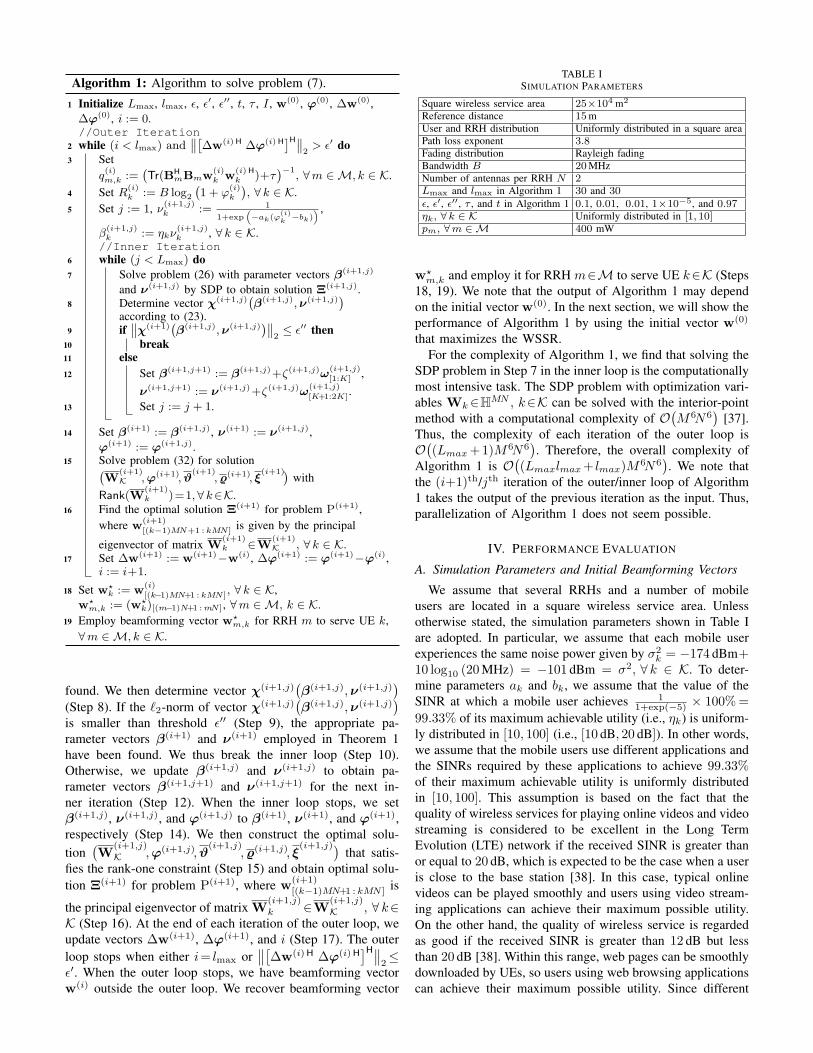
1 Initialize Lmax, lmax, ϵ, ϵ′, ϵ′′, t, τ , I , w(0), φ(0), ∆w(0),∆φ(0), i := 0.//Outer Iteration

2 while (i < lmax) and∥∥[∆w(i)H ∆φ(i)H

]H∥∥2> ϵ′ do

3 Setq(i)m,k :=

(Tr(BH

mBmw(i)k w

(i)Hk )+τ

)−1, ∀m ∈ M, k ∈ K.

4 Set R(i)k := B log2

(1 + φ

(i)k

), ∀ k ∈ K.

5 Set j := 1, ν(i+1,j)k := 1

1+exp(−ak(φ

(i)k

−bk)) ,

β(i+1,j)k := ηkν

(i+1,j)k , ∀ k ∈ K.

//Inner Iteration6 while (j < Lmax) do7 Solve problem (26) with parameter vectors β(i+1,j)

and ν(i+1,j) by SDP to obtain solution Ξ(i+1,j).8 Determine vector χ(i+1,j)

(β(i+1,j),ν(i+1,j)

)according to (23).

9 if∥∥χ(i+1)

(β(i+1,j),ν(i+1,j)

)∥∥2≤ ϵ′′ then

10 break11 else12 Set β(i+1,j+1) := β(i+1,j)+ζ(i+1,j)ω

(i+1,j)

[1:K] ,ν(i+1,j+1) := ν(i+1,j)+ζ(i+1,j)ω

(i+1,j)

[K+1:2K].13 Set j := j + 1.

14 Set β(i+1) := β(i+1,j), ν(i+1) := ν(i+1,j),φ(i+1) := φ(i+1,j).

15 Solve problem (32) for solution(W

(i+1)K ,φ(i+1),ϑ

(i+1),ϱ(i+1), ξ

(i+1))with

Rank(W(i+1)k )=1,∀ k∈K.

16 Find the optimal solution Ξ(i+1) for problem P(i+1),where w

(i+1)

[(k−1)MN+1 : kMN ] is given by the principal

eigenvector of matrix W(i+1)k ∈W

(i+1)K , ∀ k ∈ K.

17 Set ∆w(i+1) := w(i+1)−w(i), ∆φ(i+1) := φ(i+1)−φ(i),i := i+1.

18 Set w⋆k := w

(i)

[(k−1)MN+1 : kMN ], ∀ k ∈ K,w⋆

m,k := (w⋆k)[(m−1)N+1 :mN ], ∀m ∈ M, k ∈ K.

19 Employ beamforming vector w⋆m,k for RRH m to serve UE k,

∀m ∈ M, k ∈ K.

found. We then determine vector χ(i+1,j)(β(i+1,j),ν(i+1,j)

)(Step 8). If the ℓ2-norm of vector χ(i+1,j)

(β(i+1,j),ν(i+1,j)

)is smaller than threshold ϵ′′ (Step 9), the appropriate pa-rameter vectors β(i+1) and ν(i+1) employed in Theorem 1have been found. We thus break the inner loop (Step 10).Otherwise, we update β(i+1,j) and ν(i+1,j) to obtain pa-rameter vectors β(i+1,j+1) and ν(i+1,j+1) for the next in-ner iteration (Step 12). When the inner loop stops, we setβ(i+1,j), ν(i+1,j), and φ(i+1,j) to β(i+1), ν(i+1), and φ(i+1),respectively (Step 14). We then construct the optimal solu-tion

(W

(i+1,j)

K ,φ(i+1,j),ϑ(i+1,j)

,ϱ(i+1,j), ξ(i+1,j))

that satis-fies the rank-one constraint (Step 15) and obtain optimal solu-tion Ξ(i+1) for problem P(i+1), where w

(i+1)[(k−1)MN+1 : kMN ] is

the principal eigenvector of matrix W(i+1,j)

k ∈W(i+1,j)

K , ∀ k∈K (Step 16). At the end of each iteration of the outer loop, weupdate vectors ∆w(i+1), ∆φ(i+1), and i (Step 17). The outerloop stops when either i= lmax or

∥∥[∆w(i)H ∆φ(i)H]H∥∥

2≤

ϵ′. When the outer loop stops, we have beamforming vectorw(i) outside the outer loop. We recover beamforming vector

TABLE ISIMULATION PARAMETERS

Square wireless service area 25×104 m2

Reference distance 15mUser and RRH distribution Uniformly distributed in a square areaPath loss exponent 3.8Fading distribution Rayleigh fadingBandwidth B 20MHzNumber of antennas per RRH N 2Lmax and lmax in Algorithm 1 30 and 30ϵ, ϵ′, ϵ′′, τ , and t in Algorithm 1 0.1, 0.01, 0.01, 1×10−5, and 0.97ηk, ∀ k ∈ K Uniformly distributed in [1, 10]pm, ∀m ∈ M 400 mW

w⋆m,k and employ it for RRH m∈M to serve UE k∈K (Steps

18, 19). We note that the output of Algorithm 1 may dependon the initial vector w(0). In the next section, we will show theperformance of Algorithm 1 by using the initial vector w(0)

that maximizes the WSSR.For the complexity of Algorithm 1, we find that solving the

SDP problem in Step 7 in the inner loop is the computationallymost intensive task. The SDP problem with optimization vari-ables Wk∈HMN , k∈K can be solved with the interior-pointmethod with a computational complexity of O

(M6N6

)[37].

Thus, the complexity of each iteration of the outer loop isO((Lmax+1)M6N6

). Therefore, the overall complexity of

Algorithm 1 is O((Lmaxlmax+ lmax)M

6N6). We note that

the (i+1)th/jth iteration of the outer/inner loop of Algorithm1 takes the output of the previous iteration as the input. Thus,parallelization of Algorithm 1 does not seem possible.

IV. PERFORMANCE EVALUATION

A. Simulation Parameters and Initial Beamforming Vectors

We assume that several RRHs and a number of mobileusers are located in a square wireless service area. Unlessotherwise stated, the simulation parameters shown in Table Iare adopted. In particular, we assume that each mobile userexperiences the same noise power given by σ2

k = −174 dBm+10 log10 (20MHz) = −101 dBm = σ2, ∀ k ∈ K. To deter-mine parameters ak and bk, we assume that the value of theSINR at which a mobile user achieves 1

1+exp(−5) × 100%=

99.33% of its maximum achievable utility (i.e., ηk) is uniform-ly distributed in [10, 100] (i.e., [10 dB, 20 dB]). In other words,we assume that the mobile users use different applications andthe SINRs required by these applications to achieve 99.33%of their maximum achievable utility is uniformly distributedin [10, 100]. This assumption is based on the fact that thequality of wireless services for playing online videos and videostreaming is considered to be excellent in the Long TermEvolution (LTE) network if the received SINR is greater thanor equal to 20 dB, which is expected to be the case when a useris close to the base station [38]. In this case, typical onlinevideos can be played smoothly and users using video stream-ing applications can achieve their maximum possible utility.On the other hand, the quality of wireless service is regardedas good if the received SINR is greater than 12 dB but lessthan 20 dB [38]. Within this range, web pages can be smoothlydownloaded by UEs, so users using web browsing applicationscan achieve their maximum possible utility. Since different

10 16 22 28 34 40 46 52 58 640

5

10

15

20

25

30

35

40

Maximum interference constraint in multiples of noise I/σ2

Aggregate

utility

M=5,K=8, Cm=250Mbps,Γreq,k=3 dB, ε2k=0, ∀m∈M, k∈K

M=6,K=8, Cm=150Mbps,Γreq,k=3 dB, ε2k=0, ∀m∈M, k∈K

M=6,K=10, Cm=250Mbps,Γreq,k=5 dB, ε2k=0.05, ∀m∈M, k∈K

Fig. 3. Aggregate utility for different system parameters versus the normal-ized maximum interference constraint I/σ2.

applications (e.g. video streaming, web browsing) are used bymobile users, it is reasonable to assume that [10 dB, 20 dB] isthe range of the SINR at which a given user achieves 99.33%of his maximum possible utility. We thus set ak via a randomvariable that follows an inverse uniform distribution on [0.1, 1]and set bk = 5

ak, ∀ k ∈ K. Besides, vector φ(0) as well as

vector w(0) that comprises K initial beamforming vectors (i.e.,w

(0)k , ∀ k ∈K) are determined as follows. We first solve the

optimization problem after replacing the objective functionin problem (25) by

∑k∈K ηkB log2 (1 + φk) and retaining

constraints (25b) – (25e), (25g), and (25h). That is, we firstdetermine the optimal beamforming matrices that maximizethe WSSR without considering the backhaul capacity and therank-one constraint. We denote the corresponding solution as(W

(0)K , φ(0), ϑ(0), ϱ(0), ξ(0)

). Thus, the initial vector φ(0) is

determined. We then apply the approach used in Theorem 2to determine another set of rank-one matrices, denoted byW

(0)

K =W

(0)

k , k ∈ K

, which achieves the same WSSR.The beamforming vector w

(0)k is initialized by the principal

eigenvector of beamforming matrix W(0)

k , ∀ k∈K. By doingso, we not only can check the feasibility of our originalproblem for the given (Γreq,1, . . . ,Γreq,K) and (p1, . . . , pM ),but can also obtain the appropriate q

(0)m,k, ∀m∈M, k∈K, and

R(0)k , ∀ k∈K, required in the first iteration of the outer loop

of our proposed Algorithm 1. To simulate the imperfectnessof the CSI estimation, we introduce the normalized maximumchannel estimation error ε2k , ε2k/∥hk∥22,∀ k ∈ K. The CSIuncertainty region of user k is Ωk = ∆hk : ∆hH

k∆hk ≤ε2k∥hk∥22. Our results are obtained by averaging the perfor-mance of multiple path loss and small scale fading realizations.

B. Simulation Results

In Fig. 3, we show the impact of the maximum interferenceconstraint, I , in (8) on the aggregate utility. We conduct-ed simulations for network scenarios with different systemparameters, such as different numbers of users, backhaulcapacities, minimum SINRs required by mobile users, andnormalized maximum channel estimation errors. For eachnetwork scenario, we plotted the aggregate utility versus themaximum interference constraint given in multiples of noisepower σ2. That is, I was changed by tuning the ratio I/σ2.We find that the aggregate utility first increases and then

slightly decreases as I/σ2 increases. Thus, a suitable I can be

2 4 6 8 10 12 14 16 18 20 22 24 26 28 30 32 34 36 38 400

10

20

30

40

50

Index of the outer iteration in Algorithm 1 (i)

Aggregate

utility

M=10,K=14M=8,K=12M=6,K=10

Fig. 4. Convergence of Algorithm 1 for different values of M and K.Cm=150Mbps,Γreq,k=3dB, ε2k=0.05, ∀m∈M, k∈K.

obtained by running offline simulations. Even though settingI too high (i.e., I ≥ 34σ2) or too low (i.e., I ≤ 16σ2) maydegrade the aggregate utility, the aggregate utility is not verysensitive to the choice of I/σ2 in the considered interval. Weuse I = 25σ2 for the following simulations.

In Fig. 4, we illustrate the convergence of the proposedalgorithm for different numbers of RRHs (i.e., M ) and users(i.e., K). We set Cm = 150Mbps, ∀m ∈ M, and Γreq,k =3dB and ε2k = 0.05, ∀ k ∈ K. The maximum iterations Lmaxand lmax for the inner and outer loops in Algorithm 1 are set to40, respectively. The aggregate utility obtained by Algorithm 1after each iteration i of the outer loop is shown in Fig. 4. Weobserve that depending on the system parameters the aggregateutility has converged to the maximum value after about 20 to33 iterations. In particular, the larger the numbers of RRHsand users in the network, the larger the number of iterationsare required for convergence.

In Fig. 5, we present the performance of the proposedresource allocation algorithm as a function of the number ofusers in the network for six RRHs. For comparison, we alsosolve problem (6) without backhaul constraint (6c). The result-ing problem has a larger feasible set compared to problem (6).The corresponding optimal value constitutes an “upper bound”for the proposed suboptimal solution of problem (6). We alsoevaluate the aggregate utility of three baseline schemes. Inbaseline schemes I and II, we maximize the WSSR and theweighed sum of SINRs by solving problem (6) for objectivefunctions

∑k∈K ηk log2(1+γk) and

∑k∈K ηkγk, respectively.

Both problems can be solved with similar approaches asthat developed in this paper. We then use the beamformingvectors obtained for the two baseline schemes to determinethe corresponding aggregate utility for the sigmoidal utilityfunction. In baseline scheme III, we adopt the compressionstrategy proposed in [21] to solve the WSSR maximizationproblem with backhaul constraints, where similar to [21], theCSI imperfection is handled by the S-procedure [31]. We thenemploy the users’ received SINRs to determine their aggregateutility. From Fig. 5, it can be observed that the aggregate utilityincreases with the number of users. When the number of usersis increased from 4 to 6, the aggregate utility of Algorithm 1increases almost linearly. The reason for this behaviour is thatif only few users are in the system, the degrees of freedom inthe network are sufficient and all users can be properly served.However, when the number of users gets large, the co-channel

4 5 6 7 8 9 105

10

15

20

25

Number of users K

Aggregate

utility

Upper bound

Algorithm 1

Baseline scheme IBaseline scheme IIBaseline scheme III

Fig. 5. Aggregate utility versus the number of users. M = 6, Cm =150Mbps, ∀m ∈ M, ε2k = 0.05,Γreq,k = 3 dB, ∀ k ∈ K.

4 6 8 10 123

6

9

12

15

18

21

24

27

30

Number of RRHs M

Aggregate

utility

Upper bound

Algorithm 1

Baseline scheme IBaseline scheme IIBaseline scheme III

Fig. 6. Aggregate utility versus the number of RRHs. K = 7, ε2k =0.05,Γreq,k = 3 dB, ∀ k∈K, Cm = 150Mbps, ∀m∈M.

interference as well as the limited backhaul capacity hinderthe RRHs in steering the information beams accurately. Thus,the aggregate utility grows sublinearly. The performance gapbetween Algorithm 1 and the upper bound increases with thenumber of users, since the upper bound neglects the limitedcapacity of the backhaul links. Compared with the baselineschemes, we observe that Algorithm 1 achieves larger gainsin the aggregate utility as the number of users grows. Thisis because the baseline schemes may cause mismatches inresource allocation due to the nonlinear relationship betweenthe WSSR and the considered aggregate utility given by theweighted sum of sigmoidal functions. In particular, for thebaseline schemes, an exceedingly large amount of systemresources are allocated to a small set of users causing satu-ration in the sigmoidal functions, which limits the achievableaggregate utility. Moreover, a comparison of baseline schemesI and II shows that maximizing the WSSR results in a higheraggregate utility than maximizing the weighted sum of SINRssince the concavity of the logarithmic utility function in WSSRmaximization alleviates the resource allocation mismatch to acertain extent. We also observe that for large numbers of users,the data sharing strategy in baseline scheme II outperforms thecompression strategy in baseline scheme III. This is becausewhen there are more users are in the C-RAN, a coarsercompression is needed introducing more quantization noiseto accommodate all users with the capacity-limited backhaul.The received SINRs of the users in baseline scheme III arethus limited by the quantization noise.

In Fig. 6, we show the aggregate utility as a function ofthe numbers of RRHs for 7 mobile users. We find that the

aggregate utility increases with the number of RRHs for boththe proposed algorithm and the baseline schemes. Althoughthe upper bound also increases with the number of RRHs, thegap between the upper bound and Algorithm 1 shrinks as thenumber of RRHs increases. This is because the number ofbackhaul links increases with the number of RRHs and the C-RAN can support higher data rates for the mobile users. Thus,the negative impact of the limited capacity of each backhaullink on the aggregate utility is alleviated when the number ofRRHs is large. Furthermore, for M=4, the difference betweenthe aggregate utility achieved by Algorithm 1 and the baselineschemes is relatively small. This is because when M = 4,the data traffic in the network is limited by the capacity-limited backhaul in all cases. This is especially true forbaseline scheme III, as its performance is limited by the largequantization noise introduced by the compression strategy toaccommodate all users in the network. Besides, the limitednumber of antennas also restricts the available degrees offreedom for accurately steering the information beams towardsthe mobile users while satisfying their SINR requirements.However, as the number of RRHs increases, the gap betweenAlgorithm 1 and the baseline schemes widens. This is becauseAlgorithm 1 can make better use of the additional antennas andbackhaul links than the baseline schemes. The performance ofbaseline scheme III improves fast as the number of RRHsincreases. This is due to the increased degrees of freedom.Specifically, the quantization noises introduced at differentRRHs for a UE are different. An RRH which has a goodCSI estimate for a UE, introduces little quantization noiseand employs high transmission power for the UE to increaseits SINR. On the other hand, an RRH which is not in agood position to serve the UE, introduces large quantizationnoise for the UE to satisfy the capacity-limited backhaulconstraint and decreases its transmission power for the UE.Thus, baseline scheme III achieves good performance as thenumber of RRHs increases.

In Fig. 7, we investigate the impact of CSI uncertainty onthe aggregate utility. We not only compare Algorithm 1 withthe baseline schemes, but also with a non-robust beamformingdesign for aggregate sigmoidal utility maximization. Specifi-cally, the non-robust beamforming design treats the estimatedCSI as perfect information for resource allocation. Then, weoptimize w and φ for the maximization problem in (6). Inother words, robustness against CSI errors is not providedby this scheme. If the resulting resource allocation does notsatisfy the constraints for user k in (6) due to the channelestimation errors, the system is in outage and the utility ofuser k is set to zero for that channel realization to account forthe penalty of violating the constraints. We observe that theaggregate utility severely decreases when the normalized max-imum channel estimation error increases. This is because whenthe channel estimation error increases, it is more difficult forthe RRHs to accurately steer the information beams towardsthe desired users. Besides, the RRHs become less capable ofmitigating the multiuser interference. We further observe fromFig. 7 that compared to the baseline scheme, our proposedresource allocation algorithm can significantly increase theaggregate utility in C-RAN. Moreover, the proposed scheme

0 0.03 0.06 0.09 0.120

10

20

30

40

50

Normalized CSI uncertainty ε2k, ∀ k ∈ K

Aggregate

utility

Upper bound

Algorithm 1

Baseline scheme IBaseline scheme IIBaseline scheme IIINon-robust scheme

Fig. 7. Aggregate utility versus normalized maximum channel estimationerror. M=6,K=10,Γreq,k=3 dB,Cm=150Mbps, ∀ k∈K,m∈M.

50 150 250 350 4504

8

12

16

20

24

Backhaul capacity Cm, ∀m ∈ M

Aggregate

utility

Upper bound

Algorithm 1

Baseline scheme IBaseline scheme IIBaseline scheme III

Fig. 8. Aggregate utility versus the backhaul capacity of RRHs in C-RAN.M = 6, K=10, Γreq,k=3 dB, ε2k=0.05, ∀ k∈K.

achieves a significantly higher aggregate utility comparedto the non-robust beamforming design, especially for largemaximum channel estimation errors. In fact, the non-robustresource allocation scheme assumes that the available CSIis perfect and causes saturation in the utility function ofsome users and under-utilization of other users. Besides, theupper bound on the aggregate utility decreases dramaticallywhen the channel uncertainty increases. Although Algorithm1 performs better than the baseline schemes, the achievedgain in terms of the aggregate utility decreases as the channeluncertainty increases. This is because the aggregate utilitiesshown in Fig. 7 are determined based on the SINR lowerbounds taking into account the channel uncertainty. When thenormalized CSI uncertainty increases, the achievable aggregateutility and also the possible aggregate utility gain obtained byAlgorithm 1 are reduced. For baseline scheme III using thecompression strategy, the aggregate utility severely decreasesas the maximum channel estimation error increases. This isbecause the robust beamforming design has to accommodatethe worst case after the quantization noise is transmitted overuncertain wireless channels. The lower bound of the userreceived SINR in the compression strategy is thus significantlyreduced for the compression strategy.

In Fig. 8, we show the aggregate utility as a function ofthe backhaul capacity. The performance upper bound is thusshown as a horizontal line. We observe that the aggregateutility increases with the backhaul capacity of the RRHs. Thisis because a higher backhaul capacity can support higher datarates and the SINR received by each user also increases due tothe beamforming enabled by Algorithm 1. In other words, as

the backhaul capacity increases, the spatial degrees of freedomoffered by multiple RRHs can be more efficiently utilizedto increase the aggregate utility of the C-RAN. Comparedwith the baseline schemes, Algorithm 1 can significantlyimprove the aggregate utility. This is because of the resourceallocation mismatch due to the nonlinear relationship betweenthe WSSR/weighted sum of SINRs and the aggregate utility.Moreover, the aggregate utility of baseline scheme III, wherethe compression strategy is adopted, improves significantlywhen the backhaul capacity increases. This is because whenthe backhaul capacity is increased, less compression is neededand thus less quantization noise is introduced.

V. CONCLUSIONS

In this paper, we studied utility-based cooperative beam-forming design in C-RAN. We used a weighted sum of sig-moidal functions to model the aggregate utility and formulatedthe beamforming design as a non-convex optimization problemfor the maximization of the aggregate utility. Our problemformulation took into account both the imperfect CSI andthe capacity-limited backhaul. Due to the complexity of theproblem, we introduced maximum interference constraints tosimplify the optimization problem. Subsequently, an efficientiterative algorithm was proposed to obtain a good subop-timal solution. In each iteration, we tackled a non-convexoptimization problem with infinitely many constraints. Byexploiting the sum-of-ratios form of the objective function,we transformed the non-convex optimization problem intoan equivalent rank-constrained SDP problem which could besolved optimally. Simulation results unveiled that the aggre-gate utility can be significantly improved by our proposedresource allocation algorithm compared to baseline schemeswhere either the WSSR or the weighted sum of SINRs ismaximized. Furthermore, for large CSI uncertainty and alarge number RRHs compared to the number of users, theproposed suboptimal resource allocation algorithm approachedthe performance upper bound determined in the backhaulcapacity unconstrained case.

APPENDIX A: PROOF OF THEOREM 1

We present a constructive proof. We first introduce thefollowing optimization problem:

maximizeβ,w,φ,ϑ,ϱ, ξ

∑k∈K

βk (30a)

subject to ηk ≥ βk

(1 + exp (−akφk + akbk)

), ∀ k ∈ K,

(30b)constraints (7d), (18b) – (18e), and (20b),

where β , (β1, . . . , βK), βk is the auxiliary optimizationvariable for the utility of user k ∈ K, and constraint (30b)is obtained from the definition of gk(φk), ∀ k ∈ K. Problem(30) is equivalent to problem P(i+1) in the sense that ifΞ(i+1) is the solution of problem P(i+1), the solution ofproblem (30) is

(β(i+1),Ξ(i+1)

), where β

(i+1)k = gk(φ

(i+1)k ).

The Lagrangian of problem (30) is L(i+1)theo1

(β, Ξ, ν, Ψ

),∑

k∈K βk +∑

i∈K νi(ηk − βk

(1 + exp (−akφk + akbk)

))+

Θ, where ν , (ν1, . . . , νK) (ν ≽ 0) comprises theLagrangian multipliers for constraint (30b), Ξ collects alloptimization variables of problem (30) except vector β, Ψcontains the Lagrangian multipliers of all constraints in (30)except constraint (30b), and Θ denotes the sum of all termswhich are not related to vectors β and ν. Given solution(β(i+1),Ξ(i+1)

)of problem (30), the following Karush-Kuhn-

Tucker (KKT) conditions are obtained for ν(i+1) and β(i+1):

ηk − β(i+1)k

(1 + exp (−akφ

(i+1)k + akbk)

)= 0, ∀ k ∈ K,

(31a)

1− ν(i+1)k

(1 + exp (−akφ

(i+1)k + akbk)

)= 0, ∀ k ∈ K,

(31b)

where ν(i+1)k ,

(ν(i+1)k , . . . , ν

(i+1)k

)is obtained

from the solution of the dual problem of (30).On the other hand, given β(i+1) and ν(i+1), theLagrangian of problem (21) is L(i+1)

theo1

(Ξ, Ψ

),∑

i∈K ν(i+1)i

(ηk − β

(i+1)k

(1 + exp (−akφk + akbk)

))+ Θ,

where Ξ collects the optimization variables in (21), Ψ containsthe Lagrangian multipliers for the constraints in (21), and Θdenotes the sum of all terms related to Ξ and Ψ. It is easy tosee that Ξ=Ξ, Ψ=Ψ, and Θ=Θ. Thus, the KKT conditionsfor Ξ(i+1) and Ψ(i+1) for the solutions of the primary anddual problems of problem (30), respectively, are exactly theKKT conditions for problem (21). Since

(β(i+1),Ξ(i+1)

)is

the solution to problem (30) which is a convex optimizationproblem for given β(i+1) and ν(i+1), the KKT conditionsof problem (21) are sufficient for the optimality of Ξ(i+1)

in problem (21). Thus, if Ξ(i+1) is the solution to P(i+1),there exist two vectors β(i+1) =

(β(i+1)1 , . . . , β

(i+1)K

)and

ν(i+1) =(ν(i+1)1 , . . . , ν

(i+1)K

)such that Ξ(i+1) is also an

optimal solution of problem (21). Moreover, vector φ(i+1)

in Ξ(i+1) satisfies the system of equations given in (31),which is the same as the system of equations in (22). Thiscompletes the proof.

APPENDIX B: PROOF OF THEOREM 2

For the proof, we follow a similar approach as [39].If the optimal solution

(W

(i+1,j)K ,φ(i+1,j), ϑ(i+1,j),ϱ(i+1,j),

ξ(i+1,j))

of problem (26) is obtained and Rank(W

(i+1,j)k

)>

1, ∃ k ∈ K, we can construct another optimal solution thatcomprises rank-one matrices as follows. For a given φ(i+1,j)

obtained from the solution of problem (26), we solve thefollowing problem:

minimizeWK,ϑ,ϱ, ξ

∑k∈K Tr

(Wk

)(32a)

subject to Sk,1(φ(i+1,j)k , ϑk) +QH

kWkQk ≽ 0, ∀ k ∈ K,(32b)

constraints (25b), (25d) – (25h).

Problem (32) is in SDP form. Let(W

(i+1,j)

K ,ϑ(i+1,j)

,ϱ(i+1,j), ξ(i+1,j))

, where W(i+1,j)

K ,W

(i+1,j)

k | k ∈ K

, denote the optimal solution of

problem (32). It is easy to show that(W

(i+1,j)

K ,φ(i+1,j),

ϑ(i+1,j)

,ϱ(i+1,j), ξ(i+1,j))

satisfies the constraints in problem(26) and yields the same objective value as solution(W

(i+1,j)K ,φ(i+1,j), ϑ(i+1,j),ϱ(i+1,j), ξ(i+1,j)

)for problem

(26). We now show Rank(W

(i+1,j)

k

)= 1, ∀ k ∈ K. To this

end, the Lagrangian of problem (32) is given as follows:

L(i+1,j)theo2

(WK, ϑ, ϱ, ξ, Λ

)=

∑k∈K

Tr(Wk

(IMN+

∑m∈M

(λm,1+R(i)k λm,2q

(i)m,k)B

HmBm

−Qk(Lk,1+Lk,2)QHk+

∑u∈K\k

QuLu,3QHu−Vk

))−∑k∈K

Tr(Sk,1(φ

(i+1,j)k , ϑk)Lk,1

)−∑k∈K

Tr(Sk,2(ϱk)Lk,2

)−∑k∈K

Tr(Sk,3(ξk)Lk,3

)−

∑m∈M

(λm,1pm + λm,2Cm

)−

∑k∈K

ρk,1ϑk

−∑k∈K

ρk,2ϱk −∑k∈K

ρk,3ξk, (33)

where Λ ,(λ1,λ2,ρ1,ρ2,ρ3,LK,1,LK,2,LK,3,VK

)contains the dual variables. Specifically, λn ,(λ1,n, . . . , λM,n

)≽ 0, ∀n ∈ 1, 2, are the vectors of the

dual variables for constraints (25b) and (25f) in problem (32),respectively; ρn ,

(ρ1,n, . . . , ρK,n

)≽ 0, ∀n ∈ 1, 2, 3, are

the vectors of the dual variables for the constraints in (25h)in problem (32); LK,n,

Lk,n |Lk,n ∈ HMN , k∈K

, ∀n ∈

1, 2, 3, with Lk,n ≽ 0,∀ k ∈ K, n ∈ 1, 2, 3, are the sets ofdual variable matrices for constraints (32b), (25d), and (25e) inproblem (32), respectively; VK ,

Vk |Vk ∈ HMN , k ∈K

with Vk ≽ 0, ∀ k ∈ K, is the set of dual variable matricesfor constraint (25g) in problem (32). The dual problem ofproblem (32) is given as follows:

minimizeΛ

supWK,ϑ,ϱ, ξ

L(i+1,j)theo2

(WK, ϑ, ϱ, ξ,Λ). (34)

We focus on the following KKT conditions that are relevantfor our proof:

∇WkL(i+1,j)theo2

(WK, ϑ, ϱ, ξ, Λ)

∣∣∣Υ

(i+1,j),Λ(i+1,j)

= OMN ,

∀ k ∈ K, (35a)

V(i+1,j)k W

(i+1,j)

k = OMN , ∀ k ∈ K, (35b)(Sk,1(φ

(i+1,j)k , ϑ

(i+1,j)

k )+QHkW

(i+1,j)

k Qk

)L(i+1,j)k,1 =OMN ,

∀ k ∈ K, (35c)(Sk,2(ϱ

(i+1,j)k ) +QH

kW(i+1,j)

k Qk

)L(i+1,j)k,2 = OMN ,

∀ k ∈ K, (35d)

L(i+1,j)k,3 ≽ 0, ∀ k ∈ K, (35e)

W(i+1,j)

k ≽ 0, ∀ k ∈ K, (35f)

ϑ(i+1,j) ≽ 0, ϱ(i+1,j) ≽ 0, ξ

(i+1,j) ≽ 0, (35g)

λ(i+1,j)1 ≽ 0, λ

(i+1,j)2 ≽ 0, (35h)

where Υ(i+1,j) ,

(W

(i+1,j)

K , ϑ(i+1,j)

, ϱ(i+1,j), ξ(i+1,j))

and Λ(i+1,j) ,(λ(i+1,j)1 ,λ

(i+1,j)2 ,ρ

(i+1,j)1 ,

ρ(i+1,j)2 ,ρ

(i+1,j)3 ,L

(i+1,j)K,1 ,L

(i+1,j)K,2 ,L

(i+1,j)K,3 ,V

(i+1,j)K

)represent the optimal solutions of the pri-mal and dual problems in (34), respectively;∇Wk

L(i+1,j)theo2

(WK, ϑ, ϱ, ξ, Λ

)∣∣Υ

(i+1,j),Λ(i+1,j) denotes

the gradient of the Lagrangian function in (33) with respectto Wk at Υ

(i+1,j)and Λ(i+1,j). By jointly considering (35a)

and (35b), we have the following equality:

X(i+1,j)k W

(i+1,j)

k =Qk(L(i+1,j)k,1 + L

(i+1,j)k,2 )QH

k W(i+1,j)

k ,

∀ k ∈ K, (36)

where X(i+1,j)k , IMN +

∑m∈M(λ

(i+1,j)m,1 +

R(i)k λ

(i+1,j)m,2 q

(i)m,k)B

HmBm +

∑u∈K\kQuL

(i+1,j)u,3 QH

u .

Moreover, we have q(i)m,k > 0 by definition and R

(i)k > 0

due to the lower-bounded SINR Γreq,k, ∀ k ∈ K. Furtherconsidering (35e) and (35h), we have X

(i+1,j)k ≻ 0, i.e.,

Rank(X

(i+1,j)k

)=MN . Thus, we have

Rank(W

(i+1,j)

k

)=Rank

(X

(i+1,j)k W

(i+1,j)

k

)=Rank

(Qk(L

(i+1,j)k,1 + L

(i+1,j)k,2 )QH

k W(i+1,j)

k

)≤ min

Rank

(Qk(L

(i+1,j)k,1 + L

(i+1,j)k,2 )QH

k

),

Rank(W

(i+1,j)

k

), ∀ k ∈ K.

(37)

To evaluate Rank(Qk(L

(i+1,j)k,1 +L

(i+1,j)k,2 )QH

k

), ∀ k ∈ K, we

post-multiply QHk to (35c) ∀ k∈K, so

Sk,1(φ(i+1,j)k , ϑ

(i+1,j)

k )L(i+1,j)k,1 QH

k

+QHkW

(i+1,j)

k QkL(i+1,j)k,1 QH

k =OMN , ∀ k ∈ K.(38)

We then pre-multiply the LHS of (38) by[IMN 0MN

]. By

noting that Qk =[IMN hk

], we have

[IMN 0MN

]Sk,1(φ

(i+1,j)k , ϑ

(i+1,j)

k )L(i+1,j)k,1 QH

k

+[IMN 0MN

]QH

kW(i+1,j)

k QkL(i+1,j)k,1 QH

k =OMN

(a)⇐⇒ϑ(i+1,j)

k

[IMN 0MN

]L(i+1,j)k,1 QH

k

+ IMNW(i+1,j)

k QkL(i+1,j)k,1 QH

k =OMN

(b)⇐⇒ϑ(i+1,j)

k QkL(i+1,j)k,1 QH

k +W(i+1,j)

k QkL(i+1,j)k,1 QH

k

= ϑ(i+1,j)

k

[OMN hk

]⇐⇒

(ϑ(i+1,j)

k IMN +W(i+1,j)

k

)QkL

(i+1,j)k,1 QH

k

= ϑ(i+1,j)

k

[OMN hk

], ∀ k ∈ K.

(39)

In step (a), we substituted φ(i+1,j)k and ϑ

(i+1,j)

k for φk andϑk in Sk,1(φk, ϑk), respectively. Note that

[IMN 0MN

]QH

k =

IMN . Step (b) follows by adding ϑ(i+1,j)

k

[OMN hk

]on both

sides of the equation. Following similar steps in (38) and (39),we post-multiply and pre-multiply the LHS of (35d) by QH

k

and[IMN 0MN

], respectively, and obtain another equality:(

Sk,2(ϱ(i+1,j)k )+QH

kW(i+1,j)

k Qk

)L(i+1,j)k,2 =OMN

⇐⇒(ϱ(i+1,j)k IMN +W

(i+1,j)

k

)QkL

(i+1,j)k,2 QH

k

= ϱ(i+1,j)k

[OMN hk

], ∀ k ∈ K.

(40)

Without loss of generality, for UE k, we can distinguishthree cases for ϑ

(i+1,j)

k and ϱ(i+1,j)k :

Case I: ϑ(i+1,j)

k = 0 and ϱ(i+1,j)k = 0. According to (35f)

and (35g), the inverse of matrices ϑ(i+1,j)

k IMN+W(i+1,j)

k andϱ(i+1,j)k IMN+W

(i+1,j)

k exist. Further considering (39) and (40),we have

Rank(Qk(L

(i+1,j)k,1 + L

(i+1,j)k,2 )QH

k

)=Rank

(QkL

(i+1,j)k,1 QH

k +QkL(i+1,j)k,2 QH

k

)=Rank

((ϑ(i+1,j)

k (ϑ(i+1,j)

k IMN+W(i+1,j)

k )−1

+ ϱ(i+1,j)k (ϱ

(i+1,j)k IMN+W

(i+1,j)

k )−1)[OMN hk

])≤Rank

([OMN hk

])= 1.

(41)

By substituting (41) into (37), we have Rank(W

(i+1,j)

k

)≤1.

On the other hand, we have W(i+1,j)

k =OMN due to Γreq,k>0.Thus, for Case I, we have Rank

(W

(i+1,j)

k

)= 1.

Case II: ϑ(i+1,j)

k =0, ϱ(i+1,j)k =0 or ϑ

(i+1,j)

k =0, ϱ(i+1,j)k =0.

For ϑ(i+1,j)

k =0, ϱ(i+1,j)k =0, we have

W(i+1,j)

k QkL(i+1,j)k,2 QH

k = OMN . (42)

Further, considering (35a) and (35b), we have

W(i+1,j)

k

(X

(i+1,j)k −QkL

(i+1,j)k,1 QH

k

)= OMN . (43)

Since ϑ(i+1,j)

k =0,(ϑ(i+1,j)

k IMN+W(i+1,j)

k

)−1exists due to

(35f) and (35g). From (39), we have

Rank(QkL

(i+1,j)k,1 QH

k

)=Rank

(ϑ(i+1,j)

k

(ϑ(i+1,j)

k IMN +W(i+1,j)

k

)−1[OMN hk

])≤Rank

([OMN hk

])= 1. (44)

We now introduce the following lemma that facilitates ourproof:

Lemma A.1: For matrices C1 and C2 of the same size,Rank

(C1−C2

)≥ Rank

(C1

)− Rank

(C2

).

Proof: As Rank(C1) + Rank(C2) ≥ Rank(C1 + C2), itfollows that Rank(C1−C2) + Rank(C2) ≥ Rank(C1). Thus,we have Rank(C1 − C2) ≥ Rank(C1) − Rank(C2), whichcompletes the proof.

Applying Lemma A.1 to the second term of the LHS of(43), we have

Rank(X

(i+1,j)k −Qk(L

(i+1,j)k,1 )QH

k

)(45)

≥Rank(X

(i+1,j)k

)−Rank

(Qk(L

(i+1,j)k,1 )QH

k

)≥MN−1.

Thus, W(i+1,j)

k lies in the null space of matrix X(i+1,j)k −

QkL(i+1,j)k,1 QH

k which has at least rank MN − 1. Thus,

Rank(W

(i+1,j)

k

)≤1 for UE k. We also have W

(i+1,j)

k =OMN

for Γreq,k>0. Thus, Rank(W

(i+1,j)

k

)=1 for case ϑ

(i+1,j)

k =0

and ϱ(i+1,j)k = 0. A similar approach can be applied for

ϑ(i+1,j)

k = 0 and ϱ(i+1,j)k = 0 in Case II, and we conclude

that Rank(W

(i+1,j)

k

)= 1 for Case II.

Case III: ϑ(i+1,j)

k = 0 and ϱ(i+1,j)k = 0. We show by

contradiction that ϑ(i+1,j)

k =0 and ϱ(i+1,j)k =0 cannot occur.

Assume UE k ∈ K such that ϑ(i+1,j)

k =0 and ϱ(i+1,j)k =0. We

substitute ϑ(i+1,j)

k =0 and ϱ(i+1,j)k =0 into (39) and (40) for

UE k, respectively. We have

W(i+1,j)

k QkL(i+1,j)k,1 QH

k = OMN ,

W(i+1,j)

k QkL(i+1,j)k,2 QH

k = OMN .(46)

Thus, W(i+1,j)

k X(i+1,j)k =OMN , cf. (36). Since X

(i+1,j)k ≻0,

we have W(i+1,j)

k =OMN . However, W(i+1,j)

k =OMN cannotbe in the optimal solution of problem (32) due to the minimumSINR requirement of UE k. This is a contradiction. Thus,ϑ(i+1,j)

k =0 and ϱ(i+1,j)k =0 cannot occur.

Thus, each UE k ∈ K belongs to either Case I or Case II.For both cases, Rank

(W

(i+1,j)

k

)=1 has been proven, which

completes the proof.

REFERENCES

[1] Z. Wang, D. W. K. Ng, V. W.S. Wong, and R. Schober, “Transmitbeamforming for QoE improvement in C-RAN with mobile virtualnetwork operators,” in Proc. of IEEE Int’l Commun. Conf. (ICC), KualaLumpur, Malaysia, May 2016.

[2] Cisco, “Cisco visual networking index: Global mobile datatraffic forecast update, 2015-2020,” Feb. 2016. [Online]. Avail-able: http://www.cisco.com/c/en/us/solutions/collateral/service-provider/visual-networking-index-vni/mobile-white-paper-c11-520862.html

[3] D. Gesbert, S. Hanly, H. Huang, S. Shamai, O. Simeone, and W. Yu,“Multi-cell MIMO cooperative networks: A new look at interference,”IEEE J. Sel. Areas Commun., vol. 28, no. 9, pp. 1380–1408, Dec. 2010.

[4] China Mobile, “C-RAN: The road towards green radio access networks,version 2.5,” White Paper, Jun. 2012.

[5] J. Zhao, T. Quek, and Z. Lei, “Coordinated multipoint transmission withlimited backhaul data transfer,” IEEE Trans. Wireless Commun., vol. 12,no. 6, pp. 2762–2775, Jun. 2013.

[6] Y. Shi, J. Zhang, and K. Letaief, “Robust group sparse beamforming formulticast green cloud-RAN with imperfect CSI,” IEEE Trans. SignalProcess., vol. 63, no. 17, pp. 4647–4659, Sep. 2015.

[7] S. Luo, R. Zhang, and T. J. Lim, “Downlink and uplink energyminimization through user association and beamforming in C-RAN,”IEEE Trans. on Wireless Commun., vol. 14, no. 1, pp. 494–508, Jan.2015.

[8] C. Yoon and D. Cho, “Energy efficient beamforming and power allo-cation in dynamic TDD based C-RAN system,” IEEE Commun. Lett.,vol. 19, no. 10, pp. 1806–1809, Oct. 2015.

[9] F. Zhuang and V. Lau, “Backhaul limited asymmetric cooperation forMIMO cellular networks via semidefinite relaxation,” IEEE Trans. onSignal Process., vol. 62, no. 3, pp. 684–693, Feb. 2014.

[10] B. Dai and W. Yu, “Sparse beamforming and user-centric clustering fordownlink cloud radio access network,” IEEE Access, vol. 2, pp. 1326–1339, Nov. 2014.

[11] J. Segel and M. Weldon, “Lightradio portfolio — Technical overview,”Technology White Paper 1, Murray Hill, NJ, USA: Alcatel-Lucent, 2011.

[12] M. Grieger, S. Boob, and G. Fettweis, “Large scale field trial resultson frequency domain compression for uplink joint detection,” in Proc.of IEEE Globecom Workshop on Multicell Cooperation, Anaheim, CA,Dec. 2012.

[13] A. Sanderovich, O. Somekh, H. V. Poor, and S. Shamai, “Uplink macrodiversity of limited backhaul cellular network,” IEEE Trans. Inf. Theory,vol. 55, no. 8, pp. 3457–3478, Aug. 2009.

[14] A. Sanderovich, S. Shamai, and Y. Steinberg, “Distributed MIMOreceiver — Achievable rates and upper bounds,” IEEE Trans. Inf.Theory, vol. 55, no. 10, pp. 4419–4438, Oct. 2009.

[15] A. del Coso and S. Simoens, “Distributed compression for MIMOcoordinated networks with a backhaul constraint,” IEEE Trans. WirelessCommun., vol. 8, no. 9, pp. 4698–4709, Sep. 2009.

[16] L. Zhou and W. Yu, “Uplink multicell processing with limited backhaulvia per-base-station successive interference cancellation,” IEEE J. Sel.Areas Commun., vol. 31, no. 10, pp. 1981–1993, Oct. 2013.

[17] S. H. Park, O. Simeone, O. Sahin, and S. Shamai, “Robust and efficientdistributed compression for cloud radio access networks,” IEEE Trans.Veh. Technol., vol. 62, no. 2, pp. 692–703, Feb. 2013.

[18] Y. Zhou and W. Yu, “Optimized beamforming and backhaul compressionfor uplink MIMO cloud radio access networks,” in Proc. of IEEE Wire-less Optical Network Convergence in Support of Cloud Architectures,Austin, TX, Dec. 2014.

[19] O. Simeone, O. Somekh, H. V. Poor, and S. Shamai, “Downlink multicellprocessing with limited-backhaul capacity,” EURASIP J. Adv. SignalProcess, vol. 2009, pp. 3:1–3:10, Feb. 2009.

[20] P. Marsch and G. Fettweis, “On downlink network MIMO under aconstrained backhaul and imperfect channel knowledge,” in Proc. ofIEEE Global Commun. Conf. (GLOBECOM), Honolulu, HI, Nov. 2009.

[21] S.-H. Park, O. Simeone, O. Sahin, and S. Shamai, “Joint precodingand multivariate backhaul compression for the downlink of cloud radioaccess networks,” IEEE Trans. Signal Process., vol. 61, no. 22, pp.5646–5658, Nov. 2013.

[22] H. Huang, M. Trivellato, A. Hottinen, M. Shafi, P. Smith, and R. Valen-zuela, “Increasing downlink cellular throughput with limited networkMIMO coordination,” IEEE Trans. Wireless Commun., vol. 8, no. 6, pp.2983–2989, Jun. 2009.

[23] C. W. Tan, S. Friedland, and S. Low, “Spectrum management inmultiuser cognitive wireless networks: Optimality and algorithm,” IEEEJ. Sel. Areas Commun., vol. 29, no. 2, pp. 421–430, Feb. 2011.

[24] I.-W. Lai, L. Zheng, C.-H. Lee, and C. W. Tan, “Beamforming dualityand algorithms for weighted sum rate maximization in cognitive radionetworks,” IEEE J. Sel. Areas Commun., vol. 33, no. 5, pp. 832–847,May 2015.

[25] M. Xiao, N. B. Shroff, and E. K. P. Chong, “A utility-based power-control scheme in wireless cellular systems,” IEEE/ACM Trans. Net-working, vol. 11, no. 2, pp. 210–221, Apr. 2003.

[26] J.-W. Lee, R. R. Mazumdar, and N. B. Shroff, “Downlink power allo-cation for multi-class wireless systems,” IEEE/ACM Trans. Networking,vol. 13, no. 4, pp. 854–867, Aug. 2005.

[27] J. Wang and D. P. Palomar, “Worst-case robust MIMO transmission withimperfect channel knowledge,” IEEE Trans. Signal Process., vol. 57,no. 8, pp. 3086–3100, Aug. 2009.

[28] C. Shen, T.-H. Chang, K.-Y. Wang, Z. Qiu, and C.-Y. Chi, “Distributedrobust multicell coordinated beamforming with imperfect CSI: AnADMM approach,” IEEE Trans. Signal Process., vol. 60, no. 6, pp.2988–3003, Jun. 2012.

[29] C. E. Shannon, “A mathematical theory of communication,” The BellSystem Technical Journal, vol. 27, no. 3, pp. 379–423, Jul. 1948.

[30] G. Zheng, K. K. Wong, and B. Ottersten, “Robust cognitive beamform-ing with bounded channel uncertainties,” IEEE Trans. Signal Process.,vol. 57, no. 12, pp. 4871–4881, Dec. 2009.

[31] S. Boyd and L. Vandenberghe, Convex Optimization. CambridgeUniversity Press, 2004.

[32] D. Donoho, “Compressed sensing,” IEEE Trans. Inf. Theory, vol. 52,no. 4, pp. 1289–1306, Apr. 2006.

[33] E. J. Candes, M. B. Wakin, and S. P. Boyd, “Enhancing sparsity byreweighted ℓ1 minimization,” Journal of Fourier Analysis and Applica-tions, vol. 14, no. 5, pp. 877–905, Dec. 2008.

[34] M. Grant and S. Boyd, “CVX: Matlab software for disciplined convexprogramming, version 2.1,” Jun. 2015.

[35] B. Vandereycken, “Low-rank matrix completion by Riemannian opti-mization,” SIAM J. Optim., vol. 23, no. 2, pp. 1214–1236, Jun. 2013.

[36] Y.-C. Jong, “An efficient global optimization algorithm for nonlinearsum of ratios problem,” May 2012. [Online]. Available: http://www.optimization-online.org/DB FILE/2012/08/3586.pdf

[37] L. Vandenberghe, V. R. Balakrishnan, R. Wallin, A. Hansson, and T. Ro-h, “Interior-point algorithms for semidefinite programming problemsderived from the KYP lemma,” Positive Polynomials in Control, vol.312, pp. 195–238, Feb. 2005.

[38] CableFree. LTE metrics including RSRP, RSRQ and SINR.[Online]. Available: http://www.cablefree.net/wirelesstechnology/4glte/lte-rsrq-sinr/

[39] E. Boshkovska, A. Koelpin, D. W. K. Ng, N. Zlatanov, and R. Schober,“Robust beamforming for swipt systems with non-linear energy har-vesting model,” in Proc. of IEEE Int’l Workshop on Signal ProcessingAdvances in Wireless Communications (SPAWC), Edinburgh, UnitedKingdom, Jul. 2016.

Zehua Wang (S’11, M’17) received theB.Eng. degree in Software Engineering from WuhanUniversity, Wuhan, China, in 2009, the M.Eng.degree in Electrical and Computer Engineeringfrom Memorial University of Newfoundland, StJohn’s, NL, Canada, in 2011, and the Ph.D. degreefrom the University of British Columbia (UBC),Vancouver, BC, Canada, in 2016. He is currentlya postdoctoral research fellow at UBC, Vancouver,BC, Canada and the applied research engineeringscientist at Left Inc., BC, Canada. His research

interests include convex optimization, device-to-device communications,social networks, machine-type communications, and routing and forwardingin mobile ad hoc networks. He received the Chinese Government Award forOutstanding Self-Financed Students Abroad in 2015. He was the recipientof the Four Year Doctoral Fellowship (FYF) at UBC from 2012 to 2016.He was also awarded the Graduate Support Initiative (GSI) Award at UBCin 2014 and 2015. Dr. Wang served as the technical program committee(TPC) Co-chair of 2017 IEEE International Workshop on Smart Multimedia(SmartMM). He also served as the technical program committee (TPC)member for various conferences including IEEE International Conferenceon Communications (ICC), IEEE Global Communications Conference(Globecom), and IEEE Vehicular Technology Conference (VTC).

Derrick Wing Kwan Ng (S’06, M’12) receivedhis Ph.D. degree from the University of BritishColumbia (UBC) in 2012. He was a senior post-doctoral fellow at the Institute for Digital Commu-nications, Friedrich-Alexander-University Erlangen-Nurnberg (FAU), Germany. He is now working asa Lecturer and an ARC DECRA Research Fellowat the University of New South Wales, Sydney,Australia. His research interests include convex andnon-convex optimization, physical layer security,wireless information and power transfer, and green

(energy-efficient) wireless communications.

Vincent W.S. Wong (S’94, M’00, SM’07, F’16) re-ceived the B.Sc. degree from the University of Man-itoba, Winnipeg, MB, Canada, in 1994, the M.A.Sc.degree from the University of Waterloo, Waterloo,ON, Canada, in 1996, and the Ph.D. degree from theUniversity of British Columbia (UBC), Vancouver,BC, Canada, in 2000. From 2000 to 2001, he workedas a systems engineer at PMC-Sierra Inc. (nowMicrosemi). He joined the Department of Electricaland Computer Engineering at UBC in 2002 andis currently a Professor. His research areas include

protocol design, optimization, and resource management of communicationnetworks, with applications to wireless networks, smart grid, mobile cloudcomputing, and Internet of Things. Dr. Wong is an Editor of the IEEETRANSACTIONS ON COMMUNICATIONS. He has served as a Guest Editorof IEEE JOURNAL ON SELECTED AREAS IN COMMUNICATIONS and IEEEWIRELESS COMMUNICATIONS. He has also served on the editorial boardsof IEEE TRANSACTIONS ON VEHICULAR TECHNOLOGY and Journal ofCommunications and Networks. He was a Technical Program Co-chair ofIEEE SmartGridComm’14, as well as a Symposium Co-chair of IEEESmartGridComm (’13, ’17) and IEEE Globecom’13. He is the Chair ofthe IEEE Communications Society Emerging Technical Sub-Committee onSmart Grid Communications and the IEEE Vancouver Joint CommunicationsChapter. He received the 2014 UBC Killam Faculty Research Fellowship.

Robert Schober (S’98, M’01, SM’08, F’10) wasborn in Neuendettelsau, Germany, in 1971. He re-ceived the Diplom (Univ.) and the Ph.D. degrees inelectrical engineering from Friedrich-Alexander U-niversitat Erlangen-Nurnberg (FAU), Erlangen, Ger-many, in 1997 and 2000, respectively. From 2001 to2002, he was a Post-Doctoral Fellow with the Uni-versity of Toronto, Canada, sponsored by the Ger-man Academic Exchange Service (DAAD). From2002 to 2011, he was a Professor and CanadaResearch Chair with The University of British

Columbia (UBC), Vancouver, Canada. Since 2012, he has been an Alexandervon Humboldt Professor and the Chair for Digital Communication with theFAU. His research interests include the broad areas of communication theory,wireless communications, and statistical signal processing.

Dr. Schober is a fellow of the Canadian Academy of Engineering anda fellow of the Engineering Institute of Canada. From 2012 to 2015, heserved as an Editor-in-Chief of the IEEE TRANSACTIONS ON COMMUNI-CATIONS and since 2014, he is the Chair of the Steering Committee of theIEEE TRANSACTIONS ON MOLECULAR, BIOLOGICAL, AND MULTISCALECOMMUNICATIONS. Furthermore, he is a member-at-large of the Board ofGovernors of the IEEE Communications Society. He has received severalawards for his work, including the 2002 Heinz MaierLeibnitz Award ofthe German Science Foundation (DFG), the 2004 Innovations Award of theVodafone Foundation for Research in Mobile Communications, the 2006 UBCKillam Research Prize, the 2007 Wilhelm Friedrich Bessel Research Award ofthe Alexander von Humboldt Foundation, the 2008 Charles McDowell Awardfor Excellence in Research from UBC, a 2011 Alexander von HumboldtProfessorship, and a 2012 NSERC E.W.R. Steacie Fellowship. In addition,he has received several best paper awards for his research.