Page 1
The Islamic University of Gaza
Research and Graduate Affairs
Faculty of Engineering
Electrical Engineering Department
Robust Design of Thermal Solar Power Station Using
System Advisor Model (SAM) Software as the First Pilot
Project in Palestine
By:
Nader Soliman Taleb
Supervisor:
Prof. Dr. Mohammed T. Hussein
“A Thesis is submitted in Partial Fulfillment of the Requirements for the Degree of Master of
Science in Electrical Engineering“
Islamic University of Gaza, Palestine
م هـ - 2014 1435
Page 4
iv
ABSTRACT
Concentrating solar power (CSP) imposes itself as a new and efficient renewable energy
technology. This technology will be extremely helpful in improving the quality of life for many
people around the world who lack the energy needed to live a healthy life. However, the cost of
electricity from contemporary solar thermal power plants remains high, despite several decades of
development, and a step-change in technology is needed to drive down costs.
Construction of the first thermal solar power plant in Palestine is complicated by the lack of an
established, standardized and power plant configuration, which presents the designer with a large
number of choices. To assist decision making, thermo-economic studies have been performed on a
variety of different power plant configurations until reaching good results and performance.
In this thesis, a robust design of thermal solar power plant as a pilot project is designed. The design
starts with modeling the solar radiation for Gaza Strip location, reviewing different parts of the
system which are solar collectors, receivers, thermal storage system and power generation system,
and ends with designing a solar power plant for the Turkish-Palestinian friendship hospital in Al-
Zahra town with net output power of 5.40 MW. The technology of parabolic trough collector
(PTC) is chosen, then modeling of the proposed system is done using system advisor model
(SAM) software.
This thesis evaluated the designed method and shows good results in the presence of uncertainty
and the project achieved better price for electricity than the present price in Gaza Strip by a
percentage of 3.5% in addition to environmentally friendly power.
Page 5
v
.
.
04.5
(PTC) .(SAM)
540
Page 6
vi
ACKOWLEDGMENT
At the beginning, I thank ALLAH the compassionate for giving me the strength and health
to let this work see the light.
I would like express my deepest thanks to my thesis supervisor Prof. Dr. Mohammed T. Hussein,
for his support, encouragement, the time that he has spent with me as I carried out this project. His
kindness and help are appreciated.
I would like also to extend my gratitude and appreciation to thesis committee, both Dr. Hatem El-
Aydi and Dr. Iyad Abu Hadrous for their suggestions and recommendations that helped me in the
development of this research.
I express my thanks and appreciation to my family, especially my parents for raising me, their
understanding, motivation and patience.
There are no words that describe how grateful I am to my wife and my children for their
encouragement, patience and understanding me during my busy schedule.
Finally, my thanks go to anyone who helped me in one way or another in bringing out this work.
Page 7
vii
DEDICATION
To my first teacher who gave me strength … My father.
To her who planted love in my heart … My mother.
To noble spirit, for my dear life partner … My wife.
To my lovely kids … Zaina, Nada and Haya.
To the symbols of love … My brothers and sister.
Page 8
viii
TABLE OF CONTENTS
iviii ABSTRACT
vi ACKOWLEDGMENT
vii DEDICATION
viiiiii TABLE OF CONTENTS
xi LIST OF TABLES
xii LIST OF FIGURES
xiv LIST OF ABBREVIATION
1 CHAPTER ONE: INTRODUCTION
1 1.1 Introduction
2 1.2 Motivation
3 1.3 Problem statement
3 1.4 Research methodology
4 1.5 Literature review
5 1.6 Contribution
5 1.7 Thesis outline
6 CHAPTER TWO: SOLAR RADIATION
6 2.1 Introduction
6 2.2 Solar radiation fundamentals
10 2.3 Sun collector geometry
11 2.4 Available solar energy
19 CHAPTER THREE: PARABOLIC TROUGH COLLECTOR SOLAR
POWER PLANT
19 3.1 Introduction
21 3.2 PTC power plant components
Page 9
ix
22 3.2.1 Parabolic trough collector
26 3.2.2 Heat Collection Element (HCE) or receiver
27 3.2.3 Heat Transfer Fluid (HTF)
29 3.2.4 Tracking control
30 3.2.4.1 East-West tracking
31 3.2.4.2 North-South tracking
32 3.2.5 Thermal storage
36 3.3 Power generation equipment
36 3.3.1 Introduction
37 3.3.2 Parabolic trough collector power plants
38 3.3.3 Functioning of the plant
39 3.3.4 The four processes of the Rankine cycle
41 CHAPTER FOUR: PROJECT DESIGN
41 4.1 Project location (case study: The Turkish-Palestinian Friendship hospital)
43 4.2 Introduction to SAM
44 4.3 Financial Models in SAM
44 4.3.1 Residential and Commercial Projects
45 4.3.2 Power Purchase Agreement (PPA) Projects
45 4.4 Design steps in the program
45 4.4.1 Technology and financing option
45 4.4.2 Location and resource
46 4.4.3 Solar field
47 4.4.4 Collectors (SCAs)
48 4.4.5 Receivers (HCEs)
49 4.4.6 Power cycle
Page 10
x
49 4.4.7 Thermal storage
51 4.4.8 Parasitics
52 4.4.9 Performance adjustment
52 4.4.10 rough system costs
53 4.4.11 financing
54 4.5 Tracking control
55 4.6 System uncertainty
57 CHAPTER FIVE: RESULTS AND DISCUSSION
57 5.1 Introduction
57 5.2 Direct method results
66 5.3 Uncertainty effect results
70 CHAPTER SIX: CONCLUSION AND FUTURE WORK
70 6.1 Conclusion
71 6.2 Future work
72 REFERENCES
76 VITA
77 APPENDIX A
77 ((A.1): Legend colors for figure (5.13)
78 (A.2): Legend colors for figure (5.14)
79 (A.3): Legend colors for figure (5.15)
80 (A.4): Legend colors for figure (5.16)
81 APPENDIX B
81 (B.1): Completed values for Annual output vs. dirt of mirror
84 (B.2): Completed values for Annual energy vs. row spacing
88 (B.3): Completed values for Annual energy and LCOE real vs. conversion efficiency
95 (B.4): Completed values for monthly net electric output with uncertainty
Page 11
xi
LIST OF TABLES
Table (2.1): Atmospheric turbidity for Gaza Strip 13
Table (2.2): Monthly values for Gaza Strip 13
Table (2.3): Overall output data 18
Table (3.1): The four CSP technology families 19
Table (3.2): Operation conditions of contemporary solar power plants 37
Table (4.1): Electrical loads for Turkish-Palestinian friendship hospital 41
Table (4.2): Solar field parameters 46
Table (4.3): Collectors parameters 47
Table (4.4): Receivers parameters 48
Table (4.5): Power cycle parameters 49
Table (4.6): Thermal storage system parameters 50
Table (4.7): Parasitics parameters 52
Table (4.8): Performance adjustment parameters 52
Table (4.9): Trough system costs 53
Table (4.10): Financing parameters 53
Table (4.11): Parameters with uncertainty 56
Table (5.1): Output values 57
Table (5.2): Metric table for the project 65
Page 12
xii
LIST OF FIGURES
Figure (2.1): Solar angles [3]. 7
Figure (2.2): Motion of the earth about the sun 7
Figure (2.3): Angle of incidence on a parabolic trough collector 9
Figure (2.4): Displacement of the sun image 11
Figure (2.5): Location of Gaza Strip in Meteonorm software 12
Figure (2.6): Horizon for Gaza Strip 14
Figure (2.7): Diffuse and global radiations 15
Figure (2.8): Monthly temperatures 15
Figure (2.9): Precipitation and days with precipitation over a year 16
Figure (2.10): Sunshine duration and astronomical sunshine duration 16
Figure (2.11): Global radiation with uncertainty 17
Figure (2.12): Maximum and minimum daily temperature with uncertainty 17
Figure (3.1): Concentration of sunlight using (a) parabolic trough collector (b) linear
Fresnel (c) central receiver with dish (d) central receiver with distributed reflectors 20
Figure (3.2): PTC solar thermal power plant block diagram 21
Figure (3.3): Parabolic trough collector 23
Figure (3.4): One possible field arrangement 23
Figure (3.5): Parts of a Solar Collector Assembly (SCA) 24
Figure (3.6): Vacuum tube collector 26
Figure (3.7): Parabolic trough collector tracking sun path 30
Figure (3.8): N-S and E-W axis tracking 31
Figure (3.9): Two tank of molten salt for thermal energy storage 34
Figure (3.10): Two tank direct molten salt thermal energy storage 35
Figure (3.11): Two tank indirect molten salt thermal energy storage 35
Figure (3.12): Parabolic trough solar power plant 38
Figure (3.13): T-S diagram of a simple Rankine cycle 40
Figure (4.1): Site plan of the university land 42
Figure (4.2): Starting of System Advisor Model 43
Figure (4.3): Empirical sun tracker 64
Page 13
xiii
Figure (5.1): Monthly electrical output power 59
Figure (5.2): Annual electrical output power 59
Figure (5.3): Annual energy flow 60
Figure (5.4): Cost per Watt 60
Figure (5.5): Stacked real LCOE 61
Figure (5.6): Stacked nominal LCOE 61
Figure (5.7): Legend for real and nominal LCOE 62
Figure (5.8): Project after tax cash flow 62
Figure (5.9): Project cumulative IRR 63
Figure (5.10): Project cumulative NPV 63
Figure (5.11): Time series for DNI and net output electric power 64
Figure (5.12): Annual profile for DNI and net output electric power 65
Figure (5.13): Annual output vs. dirt of mirror. 66
Figure (5.14): Annual energy vs. row spacing 67
Figure (5.15): Annual energy and LCOE real vs. conversion efficiency 67
Figure (5.16): Monthly net electric output with uncertainty 68
Figure (5.17): Loss diagram for the system 69
Page 14
xiv
LIST OF ABBREVIATION
International Energy Agency IEA
Photovoltaic cell PV
Concentrated Solar Power CSP
Heat Transfer Fluid HTF
Gaza Power Generation Company GPGC
Concentrating Solar Thermal Electric System CSTES
Parabolic Trough Collectors PTC
System Advisor Model SAM
Direct Steam Generation DSG
Central Receiver Solar Power Plant CRSPP
Solar Thermal Electric Component STEC
Solar Electric Generating System SEGS
Incidence Angle Modifier IAM
National Renewable Energy Laboratory NREL
Solar Collector Assemblies SCA
Direct Normal Insolation DNI
Heat Collection Element HCE
Power of Hydrogen PH
Chlorofluorocarbon CFC
Thermal Energy Storage TES
High Pressure HP
Low Pressure LP
Power Purchase Agreement PPA
Time-Of-Delivery TOD
Levelized cost of energy LCOE
Internal Rate of Return IRR
Net Present Value NPV
Independent Power Producer IPP
Page 15
1
CHAPTER ONE
INTRODUCTION
1.1 Introduction
In our life today, problems of energy that caused by global warming and pollution effect become
important issues for researches. Renewable energy sources are considered as a technological
option for generating clean energy.
One of the most used kinds of green energy is solar energy. Solar energy shows great promise as a
renewable energy resource; it is clean, abundant, reliable, renewable, freely available and
inexhaustible. Solar energy systems are now widely used for a variety of industrial and domestic
applications especially in generating electricity. International energy agency (IEA) stated in 2010,
that the net consumption of electricity power generated from renewable energy sources increases
over time to become by 2015 the major portion [1].
Solar system is based on a solar collector, designed to collect the sun’s energy and to convert it
into either electrical power or thermal energy. In the space of ninety minutes, enough sunlight
strikes the earth’s surface will fuel the world’s energy needs for a full year. The only problem on
the way of using solar power plants is the high cost of setting up and operating them. So among
some ways of controlling and monitoring of these systems, those will lower costs and hold good
reliability for these systems.
Because the sun radiation to the ground affected by the climate, latitude, longitude and other
natural conditions, it put higher requirements for collection and utilization of solar energy. The use
of automatic sun tracking device to improve the utilization of solar energy is an important way.
Theoretical analysis shows that there is difference of about 37% between the solar panel tracking
energy and non-tracking [2].
The use of a tracking mechanism increases the amount of solar energy received by the solar
collectors resulting to a higher output power. The available amount of solar energy also depends
upon the location. In general, the amount of usable solar energy is contingent upon the available
solar energy, other weather conditions, the technology utilized, and the intended application.
Solar power plant work to convert sunlight into electricity, either directly using photovoltaic cells
(PVs), or indirectly using concentrated solar power (CSP). CSP systems use either lenses or
Page 16
2
mirrors and tracking systems to focus a large area of sunlight into a small beam, while PVs convert
light into electric current using the photoelectric effect.
CSP is one of such renewable energy sources which came into light in the late 20th
and early 21st
century [3]. Initially, CSP was used for small scale solar thermal-mechanical applications, with
outputs reaching up to 100 Kilowatt (KW), mainly for water pumping. Only after the energy crises
of 1973 did the idea of large-scale solar power plants took hold.
In CSP technology, the incident solar radiations are reflected onto the receiver placed at the focal
point (or along the focal line, in case of line-focusing CSP) to increase the temperature of the
surface up to even 1400 ºC. The gained heat energy by heat transfer fluid (HTF) or working fluid
is then transformed into the usable form of energy such as electricity using turbines and generators.
Today, CSP represents a reliable technology for electricity generation with a global installed
capacity that exceeds the 2 Giga watt electrical (GWe).
In September 2013, the biggest solar thermal power plant was fired up in California, which is once
fully operational. The project is expected to produce 377 Megawatt (MW) of net power and during
some days it could provide enough power for more than 200,000 homes. India will also build the
largest solar plant in the world to generate 4000 MW from sunlight near the Sambhar lake in
Rajasthan with the intention to finish the first part of the project in 2016 with net power reaching
up to 1000 MW. These projects reflect the world moving towards CSP technology to generate
electricity and use renewable energy rather than fossil fuels.
1.2 Motivation
In recent years, Gaza Strip suffers from limited electric sources that due to problems in Israeli
feeders or lack of fuel for Gaza power generation company (GPGC), which lead people to find
alternative solution to this problem using small generators, inverters and solar cells.
The provision of a sustainable energy supply is one of the most important issues facing humanity
at the current time, and solar thermal power has established itself as one of the more viable sources
of renewable energy. Also, it achieves better efficiency than PV cells.
In addition to the electrical problem presented, Gaza Strip is 360 km2 and has an excellent
solar location with 2135 kWh/m2/year irradiation [4]. These reasons motivated me to investigate
the theoretical performance of a concentrating solar thermal electric system (CSTES) using a field
of Parabolic Trough Collector (PTC). This thesis presents a design of thermal solar power station
Page 17
3
with self-tracking mechanism for the Turkish-Palestinian Friendship Hospital at the Islamic
University land located in Al-Zahra town with net power of 5.40 MWe. The design is made using
System Advisor Model (SAM) software which presents economic feasibility study for the project
in addition to the technical design.
1.3 Problem statement
As it is well known in our country, there is a big problem in electrical power generation, since
sources of electricity are limited and are not enough to meet all people requirements. Also, we see
that a lot of countries moving toward using thermal solar power plants in producing electricity.
For this reasons, this thesis seeks to find alternative solution for electric power problem that we
face in Gaza Strip, so that, it presents theoretical performance of PTC, and then apply this
technique on the Turkish-Palestinian Friendship Hospital at the Islamic University land as a case
study. This work can be applied practically (if the funding available) so that we can get electricity
for the hospital with efficient and clean method. Note that, this project can apply to any location in
our country if area and fund are available.
1.4 Research methodology
In this thesis, systematic modeling and design procedures for overall PTC solar substation are
developed. The procedure of this thesis is as follows:
1. Collecting wanted data about the research subject from related papers, books, journals,
previous researches and internet.
2. Modeling the weather data base for Gaza Strip using Meteonorm software with help of Bet
Dagan weather database to use it in simulation part.
3. Modeling and design the different parts of our system, which are the parabolic trough
collector, receiver, thermal storage and power generation system in the presence of
uncertainty affected on the system.
4. Implementing the proposed thermal solar power plant on SAM software with self-tracking.
5. Testing the system and check results obtained from overall system.
Page 18
4
1.5 Literature review
Several researches were proposed in this field as shown below:
R. Desai proposed a study of thermo-economic analysis of a solar thermal power plant with
a central tower receiver for Direct Steam Generation (DSG). The goal of his study was to
evaluate the thermodynamic and economic performance of one of these plants by
establishing a dynamic simulation model and coupling it with in-house cost functions. He
proved that these plants had the benefit of working with a single HTF and reached to higher
temperatures than conventional parabolic trough CSP plants. This increased the efficiency
of the power plant. He used the TRNSYS simulation studio together with MATLAB for
post processing calculations and achieved good results [5].
O. H. Abdulla et. al presented steady state and transient studies to assess the impact of
a 200 MW central receiver solar power plant (CRSPP) connection on the main
interconnected transmission system of Oman. They proposed the 2015 updated
transmission grid model and included the simulation of the proposed 200 MW CRSPP
using the DIGSILENT power factory professional software. Their results were shown that
the steady state and transient responses for the proposed plant were acceptable [6].
Y. Usta investigated the theoretical performance of a CSTES in Turkey using a field of
PTC. She used the commercial software TRNSYS and the Solar Thermal Electric
Component (STEC) library to model and simulate the overall system. The model was
constructed using data for solar electric generating system (SEGS) VI. She found good
agreement between the model’s predictions and published data with errors usually less than
10%. Also, she compared the output results for two systems in terms of absolute monthly
outputs and in terms of ratios of minimum to maximum monthly outputs [7].
M. Dicorato et, al investigated a concentrating solar trough plant, having nominal power
equal to 100 KWe and exploiting linear PTC to generate electricity by means of Organic
Rankine cycle turbine. They developed a model to estimate solar radiation on a sun
tracking surface, in order to minimize the angle of incidence and thus maximize the
incident beam radiation. Also, they examined a suitable inclination of the North-South
rotation axis on the horizontal plane. They proved that, tracking system with inclined
rotation axis on the horizontal plane have yielded better results compared with those from
biaxial sun tracking [8].
Page 19
5
M. Jahromi et. al presented modeling for the linear parabolic solar power plant via system
identification, and nonlinear model for Shiraz solar power plant. In the proposed model, the
input and output were assumed to be the entering oil flow and outgoing oil temperature.
The ARX linear model was proposed and evaluated with the use of input-output data, noise
and disturbance. In addition, they calculated the input, output, and delay coefficient in
optimized state by applying MATLAB software. Their results showed that the method they
used it was efficient [9].
Jones et al. developed a detailed performance model of the 30 MWe SEGS VI parabolic
trough plant which was created in the TRNSYS simulation environment using the STEC
model library. The power cycle and solar collector performance were modeled, but unlike
the actual system natural, gas-fired hybrid operation was not modeled. Good agreement is
obtained when comparing the results of their model with plant measurements, and errors
percentages were less than 10% [10].
1.6 Contribution
This research of thermal solar power system is very useful and attractive for many researchers and
practitioners especially for electrical engineers. According to the issues related to electric power
demand, design and evaluation process of the system has been developed here step by step using
SAM software, which is a great program for this field.
Developing thermal solar power plant in Gaza Strip for the first time with feasibility study for
building real system for the Turkish-Palestinian Hospital at the Islamic University of Gaza is
considered main contribution to this research.
1.7 Thesis outline
There are six chapters in this thesis; Chapter 2 presents the study of solar radiation fundamentals
and solar data for Gaza Strip obtained by Meteonorm software. Chapter 3 covers briefly the
parabolic trough collector solar power plant components. Chapter 4 presents input parameters for
each section of the system in SAM software. Chapter 5 demonstrates results for the design of a
thermal solar power plant for the Turkish-Palestinian hospital with the presence of uncertainty in
system parameters. Finally chapter 6 ends up with conclusion, recommendations, and future work.
Page 20
6
CHAPTER TWO
SOLAR RADIATION
2.1 Introduction
Detailed information about solar radiation availability at any location is essential for the design
and economic evaluation of parabolic trough solar power plants. Therefore, precise knowledge of
historical global solar radiation at a location of study is required for the design of any funded solar
energy project. Long term measured data of solar radiation are available for a large number of
locations in different parts of the world.
Unfortunately, no meteorological stations are available in Gaza Strip to measure the amount of
intercepted solar radiation in Gaza Strip. So an alternative method for estimation of solar radiation
is required, and different satellite models can be used to estimate the solar energy availability.
Note that, according to [11] the solar radiation level for both areas Gaza Strip and Bet Dagan are
similar, so, the weather database available for Bet Dagan can be slightly changed by data obtained
from Meteonorm software and used it in this thesis to represent weather data for Gaza Strip.
The energy contained in the direct normal radiation is harvested by the concentrating collectors of
a solar field. By reflecting the received normal direct radiation to the absorber, thermal energy is
produced and transported to the power block. Conventional technology is used to convert this
energy into electrical energy. Therefore the incoming radiation can be seen as the fuel of a CSP
plant. For a precise calculation of the CSP plant performance, it is essential to understand the
geometrical relations between the sun and earth at any time of the day.
2.2 Solar radiation fundamentals
As a study of solar radiation that strikes the earth's surface, some definitions must be known.
It is important to introduce some definitions for beam radiation angles. These angles describe the
relationship between the oncoming sun radiation from the sun and any plane on the earth with a
specific position. Figure (2.1) shows some of these angles.
Page 21
7
Figure (2.1): Solar angles [3].
The variation in seasonal solar radiation availability at the surface of the earth can be understood
from the geometry of the relative movement of the earth around the sun. The distance between the
earth and the sun changes throughout the year, the minimum being 1.471 × 10¹¹
m at winter
solstice (December 21), and the maximum being 1.521 × 10¹¹
m at summer solstice (June 21). The
year round average earth-sun distance is 1.496 × 10¹¹
m. The amount of solar radiation intercepted
by the earth, therefore varies throughout the year, the maximum being on December 21, and the
minimum on June 21 as shown in figure (2.2) [12].
Figure (2.2): Motion of the earth about the sun.
The axis of the earth’s daily rotation around itself is at an angle of 23.45 ° to the axis of its ecliptic
orbital plane around the sun. This tilt is the major cause of the seasonal variation of the solar
radiation available at any location on the earth. In this regards, important information about this
angles should be known.
Page 22
8
Latitude (ϕ) is the location of site we interested in with respect to the equator, where ϕ
varies from -90 in South to +90 in North.
Declination angle (δ) is the angle between the earth-sun line (through their center) and the
plane through the equator. The declination angle varies between -23.45° on December 21 to
+23.45° on June 21. The solar declination angle is given by equation (2.1).
( ( )
) ( )
Where n is the day number with January 1 being n = 1 to 31st December being n = 365.
In general, the declination is assumed to remain constant during a specific day. The
analysis of the sun motion is based on the Ptolemaic theory, which assumes that the earth is
fixed and the sun rotates around the earth. The Ptolemaic view describes the relative sun
motion with a coordinate system fixed to the earth with its origin at the location of interest.
Hour angle (ω) is the angular presentation of hour for solar time. It is based on the
nominal time of 24 hours required for the sun to move 360° around the earth (or 15° per
hour). ω = 0 at 12:00 solar noon, and in the range of -180 ≤ ω ≤ 180 before and after 12:00.
The solar hour angle can be calculated from equation (2.2).
( ) ( )
Where ts is the solar time in hours. The solar time is calculated from the local time by
equation (2.3) [12].
( ) ( )
Where lst is the standard time meridian, llocal is the local time meridian and EOT is the
equation of time, which accounts for the variation of the rotational speed of the earth. An
approximation for calculating EOT in minutes is given by Woolf [13], and is accurate to
within about 30 seconds during daylight hours.
( ) ( ) ( ) ( ) ( )
Where x can be calculated as:
( )
( )
Slope (β) is the angle between the horizontal surface and the inclined plane. By another
expression, it is the tilt angle.
Page 23
9
Surface azimuth angle (γ) is the angle between the projection of the plane on horizontal
and the south direction. This angle has a range of -180 ≤ γ ≤ 180 from East to West.
Solar azimuth angle (γs) is the angle between a due south line and the horizontal
projection of the line joining the site to the sun. The sign convention used for azimuth angle
is positive for West of South and negative for East of South. Solar azimuth angle can be
calculated using equation (2.6).
( ( ) ( )
( )) ( )
Solar altitude angle (αs) is the angle between a line collinear with the sun rays and the
horizontal plane. Equation (2.7) is used to calculate the solar altitude angle.
( ( ) ( ) ( ) ( ) ( )) ( )
Zenith angle (θz) is the angle between the oncoming beam radiation and the normal on
the horizontal surface. It is the complement of altitude angle.
( )
Angle of incidence (θ) is the angle between the oncoming beam radiation and the normal
on an inclined surface. Figure (2.3) illustrates the angle of incidence between the collector
normal and the beam radiation on a parabolic trough. The angle of incidence results from
the relationship between the sun’s position in the sky and the orientation of the collectors
for a given location.
Figure (2.3): Angle of incidence on a parabolic trough collector [14].
Page 24
10
The relation between the angle of incidence and the solar position angles for the plane of
collector aperture is given by equation (2.9) [15].
( ) ( ) ( ) ( ) ( ) ( ) ( ) ( )
( ) ( ) ( ) ( ) ( ) ( ) ( ) ( ) ( )
( ) ( ) ( ) ( ) ( )
For horizontal surface (β = 0), the incidence angle = zenith angle as in equation (2.10).
( ) ( ) ( ) ( ) ( ) ( ) ( )
2.3 Sun collector geometry
For the operation of a CSP plant, temperatures of around 400°C are necessary. These high
temperatures cannot be reached with a flat plate collector, therefore concentrating collectors are
used. The direct normal radiation reaching the collector is concentrated on the absorber tube
located in the focal point of the parabolic collector. The most important characteristic factor
therefore is the concentration ratio. It is defined as the aperture area in relation to the absorber area
as shown in equation (2.11) [16].
( )
Where Aa is the aperture area of parabolic collector, and Aabs is the area of the absorber.
The PTC is a two dimensional system, so a maximum concentration ratio can be reached to 200.
The main effect on the concentration ratio is losses, and the most significant losses under some
circumstances occurring in a solar field are the shading losses. This reduction is happened when
one collector row reflects their shadow onto the next row.
Another loss factor occurs because the incoming radiation to the collector is not exact
perpendicular, and the absorber tube has a finite length. At the end of each collector, a certain part
of the absorber tube will not be irradiated. This displacement of sun image is shown in figure (2.4).
In the northern hemisphere, these effects can be noticed especially during winter time. Normally
these losses are under two percent in feasible areas for CSP plants.
Further losses that occur depend on the finite earth-sun distance, where the beams reaching the
collectors are also not exactly parallel. As a result, the sun image on the absorbers is not precisely
circular. The image can be seen in the form of an ellipse, which changes the frame, depending on
the angle of incidence.
Page 25
11
Figure (2.4): Displacement of the sun image.
By increasing the incidence angle, the performance characteristic of the sun image becomes worse.
This happens because the absorber is designed for a perfect circular sun image. This effect is called
Incidence Angle Modifier (IAM), and can be predicted in general according to [16].
( ) ( )
The irradiation reaching the collector can be separated in two parts. One is exactly perpendicular to
the other, and one is horizontal to the collector. The collector however only can reflect the
perpendicular part of the radiation. This leads to the so called cosin-effect. The amount of useful
irradiation can be calculated according to [17] by equation (2.13).
( )
2.4 Available solar energy
In every moment, the fraction of the radiant flux that reaches a specific location on the Earth’s
surface is highly variable, depending upon local atmospheric conditions and cloud cover.
Meteorological science has not yet advanced to the point at which it is possible to obtain detailed
forecasts of weather conditions more than a few days into the future. As such, it is impossible to
predict the available solar radiation on a daily basis.
The design of solar power systems must therefore rely on long-term statistical averages, which
permit evaluation of the suitability of a site for the production of solar energy. The variable nature
of the solar resource means that at least 10 years of meteorological data should be used when
evaluating a potential site, in order to remove statistical anomalies.
In this thesis, Meteonorm software is used to determine the location of Gaza Strip and to obtain
solar information about the location that intended to design the substation on it.
Page 26
12
Meteonorm is primarily a method for the calculation of solar radiation on arbitrarily orientated
surfaces at any desired location. The method is based on databases and algorithms coupled
according to a predetermined scheme. It commences with the user specifying a particular location
for which meteorological data are required, and terminates with the delivery of data of the desired
structure and in the required format.
The first step in the software is to determine Gaza Strip location on the map, then the program
determine the latitude and longitude as shown in figure (2.5).
According to [18], the optimal values for azimuth and tilt angles are 180° and 31.42° respectively,
so it is used in the program as input parameter, and determine the inclination angle to be equal 45°.
Figure (2.5): Location of Gaza Strip in Meteonorm software.
After that, the program shows the atmospheric turbidity as uncertain parameter that effect on the
solar beam radiation as shown in table (2.1). Aeronet results indicate to the nearest station from the
chosen location which in our case is Nes Ziona with latitude = 31.9°, longitude = 34.8°, and 55
Km far from Gaza Strip.
Page 27
13
Table (2.1): Atmospheric turbidity for Gaza Strip.
Month Interpolated Aeronet Custom
January 3.45 3.51 3.45
February 3.45 4.00 3.45
March 3.90 4.38 3.90
April 4.56 5.28 4.56
May 4.32 4.84 4.32
June 3.39 3.63 3.39
July 3.68 4.17 3.68
August 3.51 4.09 3.51
September 3.51 4.07 3.51
October 3.85 4.34 3.85
November 3.51 3.7 3.51
December 3.51 3.61 3.51
Year 3.72 4.14 3.72
Then, the weather monthly values for Gaza Strip for the year 2013 can be downloaded from
internal tool in the program. Table (2.2) shows these values.
Table (2.2): Monthly values for Gaza Strip.
Month Ta Tadmin Tadmax Tamin Tamax
January 13.1 8.1 18.9 3.5 28.4
February 15 9.9 20.9 6.2 28.7
March 18 11.6 25 6.5 37.1
April 19.7 13.4 25.7 9.2 37.4
May 23.3 17.4 29.7 13.3 38.4
June 25.8 20.4 31.2 15.7 40.1
July 26.7 22.6 31.3 20.3 35.1
August 27.6 23.1 32.3 20.9 34.2
September 26.2 21.7 30.9 16.9 35.3
October 22 16.5 27.9 11.9 31.8
November 20.3 14.8 27 11.2 35.3
December 13.4 8.7 19.6 1.9 30.2
Where Ta is the temperature, Tadmin/max is the mean daily minimum/maximum of temperature and
Tamin/max is the minimum/maximum hourly temperature.
Page 28
14
Note that the influence of the horizon profile on the monthly and hourly values is taken into
account. For hourly values, a relatively little elevated horizon may already have a strong influence
on individual values. For these reasons, it is important to consider the effects of a raised horizon.
Figure (2.6) is taken from the program, and shows the horizon for Gaza Strip.
Figure (2.6): Horizon for Gaza Strip.
Where the x-axis represents the azimuth angle, y-axis represent the elevation angle and curves
represent the sun path. After the above procedure done, the results are obtained as shown below.
Page 29
15
Figure (2.7): Diffuse and global radiations.
Figure (2.8): Monthly temperatures.
Page 30
16
Figure (2.9): Precipitation and days with precipitation over a year.
Figure (2.10): Sunshine duration and astronomical sunshine duration.
Note that, the program takes uncertainty range of yearly values as follow:
Gh=6%, Bn=11%, Gk=8%, Ta=0.8°C and variability of Gh/year: 3.4%
Page 31
17
Where Gh is the global radiation horizontal, Bn is the beam radiation, Gk is the global radiation on
inclined surface.
Figure (2.11): Global radiation with uncertainty.
Figure (2.12): Maximum and minimum daily temperature with uncertainty.
The total results obtained from the program are shown in table (2.3).
Page 32
18
Table (2.3): Overall output data for Gaza Strip.
Month Gh
KWh/m2
Gk
KWh/m2
Dh
KWh/m2
Bn
KWh/m2
Ta
°C
Td
°C
FF
m/s
January 106 25 36 152 13.1 8 3
February 114 32 45 128 13.8 8.3 3
March 169 69 59 175 16 9.9 3.4
April 191 115 68 180 20 12.2 4
May 224 167 78 209 22.8 14.7 4
June 230 184 68 228 25.8 18.3 4
July 234 181 70 232 27.7 21 4
August 216 141 68 212 27.9 21.6 3.9
September 185 88 52 202 26.2 20.4 3.1
October 149 42 47 181 23.3 17.4 2.8
November 113 24 34 156 18.9 12.7 2.5
December 98 23 32 147 14.6 9.6 2.9
Year 2029 1091 657 2202 20.84 14.51 3.38
Where Dh is the diffuse radiation horizontal, Td is the dew point temperature and FF is the wind
speed.
As mentioned previously, Gaza Strip does not have meteorological station; hence, the program
depends on interpolation technique in calculation. The interpolation depends on the following
locations:
Radiation interpolation locations: Gilat (27 Km), Bet Dagan (64 Km), El Arish (80 Km),
Dead Sea (94 Km), Jerusalem (78 Km).
Temperature interpolation locations: Gilat (27 Km), Bet Dagan (64 Km), Ben-Gurion
airport (69 Km), Beer-Sheva/Teyman (43 Km), El Arish (80 Km).
Finally, as it presented before, the output data obtained from Meteonorm will be taken and put in
Bet Dagan weather database to represent the weather data for Gaza Strip in simulation part of this
thesis in chapter four.
Page 33
19
CHAPTER THREE
PARABOLIC TROUGH COLLECTOR
SOLAR POWER PLANT
3.1 Introduction
CSP is a large-scale, commercial way to generate electricity through solar energy. CSP systems
comprise concentrated solar radiation as a high temperature thermal energy source to produce
electrical power. CSP systems produce heat or electricity using hundreds of mirrors/reflectors to
concentrate the solar radiation to a temperature typically between 400oC and 1000
oC. This thermal
power triggers Rankine, Brayton or Sterling cycles, and finally mechanical energy is converted to
electricity through an electric generator which is further injected in to the transmission grid. CSP is
being widely commercialized with about 1.17 GW of CSP plants online as of 2011 and about
17.54 GW of CSP projects are under development worldwide [5]. At present, there are four main
CSP technologies, which can be categorized by the way they focus the sun’s rays and the
technology used to receive the sun’s energy (table 3.1).
Table (3.1): The four CSP technology families.
Focus type () Line focus Point focus
Receiver type ()
Collectors track the
sun along a single axis
and focus irradiance
on a linear receiver.
Collectors track the
sun along two-axis and
focus irradiance at a
single point receiver.
Fixed
Fixed receivers are stationary devices
that remain independent of the plant's
focusing device. This eases the
transport of heat to the power block.
Linear Fresnel
Collectors
Central Receiver
System
Mobile
Mobile receivers move together with
the focusing device. In both line focus
and point focus designs, mobile
receivers collect more energy
Parabolic Trough
Collectors Parabolic Dishes
Page 34
20
The main four CSP technologies are parabolic trough collectors, central tower, linear fresnel and
parabolic dishes as shown in figure (3.1). One of the most evolved technologies is the parabolic
trough collectors. It is being used in several power plants over the world and proposed in plans for
new plants. High temperatures can be achieved in central receiver power plants, promising high
efficiency conversion ratios from solar to electricity; however, the cost of this technology is still
expensive caused by its limited production.
Figure (3.1): Concentration of sunlight using (a) parabolic trough collector (b) linear Fresnel (c)
central receiver with dish (d) central receiver with distributed reflectors [19].
In this thesis, the technology of PTC is chosen, and then modeling of the proposed system using
the computer software SAM is presented. SAM represents the performance and the cost of
renewable energy projects using computer models developed at National Renewable Energy
Laboratory (NREL), Sandia National Laboratories, the University of Wisconsin, and other
organizations. Each performance model represents a part of the system, and each financial model
Page 35
21
represents a project's financial structure [20]. The models require input data to describe the
performance characteristics of physical equipment in the system and project costs.
In this chapter, theoretical background for PTC power plant is proposed with detailed information
about each part of the system.
3.2 PTC power plant components
PTC systems are the most developed systems among all concentrating solar thermal power
technologies. Today, most of the solar thermal power plants use parabolic trough collector
systems. The block diagram of the proposed system is shown in figure (3.2), which consists of
PTC having parabolic reflective mirrors, receiver (absorber tubes) for concentrated radiation,
thermal storage system and power generation equipment. PTC systems use a Rankine cycle to
produce electricity.
Figure (3.2): PTC solar thermal power plant block diagram.
PTC system consist of parallel rows of mirrors (reflectors) curved in one dimension to focus the
sun’s rays. Stainless steel pipes (absorber tubes) with a selective coating serve as the heat
collectors. The coating is designed to allow pipes to absorb high levels of solar radiation while
emitting very little infrared radiation. The pipes are insulated in an evacuated glass envelope.
The dynamics of the distributed solar collector field are described by the following system of
partial differential equations describing the energy balance [21].
Page 36
22
( ) ( ) ( )
( ) ( )
Where the sub-index refers to the metal, and to the fluid. represents the sum of radiative
and conductive thermal losses, and are the density of the metal and fluid respectively,
and are the heat capacities, and are the tube cross section and inner area, is the solar
radiation, is the reflectivity coefficient, is the oil flow and , and are metal, fluid and
ambient temperatures respectively.
Now the detailed theoretical background for each part of our system is discussed.
3.2.1 Parabolic trough collector
A parabolic trough is a type of solar thermal collector that is straight in one dimension and curved
as a parabola in the other two. The collectors are constructed as long parabolic mirrors, which have
a thickness of approximately 4 mm and are typically coated by silver or polished aluminum to
maximize the reflectance of the incoming rays. The mirrors used as concentrator consist of a heat-
formed glass cake. It is carried by the metal structure of the collector. By using special production
techniques, like the float-glass method, absolute evenness of the cake is guaranteed. Glass, which
is used in solar applications, must have very low iron content for getting a transmissivity in the
solar spectrum of around 91%. The iron content of a so-called “White Glass” is around 0.015%
compared to normal glass with an iron content of around 0.13%, so it can be best choice in solar
power plant [22].
The energy of sunlight which falls into the mirror parallel to its plane of symmetry is focused
along the focal line, where HTF inside the receiver is positioned that is intended to be heated.
Figure (3.3) shows the parabolic trough collector.
The group of collectors in solar power plant is called solar field. The solar field is the heat
collecting portion of the plant. It consists of many parallel rows of solar collectors aligned on a
north-south horizontal axis. In order to reach the operational conditions, the solar collector
assemblies (SCA) are arranged in a series configuration normally known as a loop [23].
A common header pipe provides each loop with an equal flow rate of HTF, and a second header
collects the hot HTF to return it either directly to the power cycle for power generation or to the
thermal energy storage system for use at a later time.
Page 37
23
Figure (3.3): Parabolic trough collector.
To minimize pumping pressure losses, the field is typically divided into multiple sections, each
section with its own header set, and the power cycle is situated near the middle of the field. Figure
(3.4) shows one possible plant layout where two header sections are used for 20 total loops.
The solar field produces thermal energy by using direct normal insolation (DNI), and delivers this
energy to a steam power plant. DNI can be evaluated using relation (3.3).
∫ ( ) ( )
Where is the beam radiation, which is incident from the direction of the center of the sun’s
disk. The total irradiation on the field is a function of the equivalent aperture area of all of the
collectors in the field, the strength of the solar insolation, and the angle at which the irradiation
strikes the aperture plane.
Figure (3.4): One possible field arrangement.
Page 38
24
Note that it is commonly accepted that the minimum DNI at which it becomes economically viable
to build a concentrating solar power plant is around 2000 kWh/m2, and particularly in Palestine,
DNI reach to average value of 2400 kWh/m2 [4].
One of the most modern Collectors nowadays is the type LS-3. One LS-3 collector consists of 224
mirror segments, where each segment has an area of 2.68 m2. Taking into consideration the
bending of the mirrors, an area of 545 m2 is reached with one LS-3 collector. In addition, the
collector contains 24 absorber tubes [24].
Traditionally, a steel truss is used as the frame (LS-3 and LS-2 space frame), although other
approaches such as torque tubes (Euro Trough) and lighter metals (Duke Solar space frame) are
being explored. The support structure with drive controls is shown in Figure (3.5) [25].
Figure (3.5): Parts of a Solar Collector Assembly (SCA).
When we talk about PTC, a very important definition must be presented, which is the equivalent
aperture area. It refers to the total reflective area of the collectors that is projected on the plane of
the collector aperture. This area is distinct from the curved reflective surface. Area that is lost due
to gaps between mirror modules or non-reflective structural components is not included in the
aperture area value. Thus, though the structure of the collector may occupy 100 m lengthwise and
5 m across the aperture, for example, the total reflective aperture area may be somewhat less than
100 × 5 = 500 m2 after spaces, gaps, and structural area are accounted for.
The parabolic reflector is defined by its aperture diameter (W), rim angle (θr), and receiver shape
and size. The radius of parabola at an arbitrary location is defined by r, and is called the mirror
radius. The maximum mirror radius occurs at its outer rim and is fittingly called rim radius or
Page 39
25
parabolic radius. The rim angle θr corresponds to beam radiation reflected from the outer rim of
the concentrator. The focal length f is related to rim angle and aperture width as in equation (3.4)
[26]:
(
) ( )
The size of a reflected solar image at the focal point depends upon the mirror radius at the point of
incident of the beam radiation. A simple equation for the image width Wim was developed by Jeter
[27].
( )
Where θs represents the angular width of the incident beam radiation of 0.53o (≈ 0.00925 rad) with
an acceptance half angle θa of 0.267o, and reflected beam path length equal to the parabolic radius
r, then for near normal incidence, occurring more frequently in the summer months, equation (3.5)
can be rewritten as:
( )
The concentration ratio C which is written in equation (2.13) is related to θr, can also defined as:
( )
The size of the receiver to intercept the entire solar image can be calculated. The diameter Dr of a
cylindrical receiver is given by: [28]
( )
For a flat receiver in the focal plane of the parabola, the width Wf is given by:
( )
( ) ( )
Now, the optical analysis of solar collectors with parabolic reflector must take into account. There
are many different effects such as optical properties of materials, relative size of receiver and
concentrator, the type of tracking and the corresponding losses.
Optical Efficiency of PTC
The optical efficiency ηo is the fraction of solar radiation incident on the aperture of the collector
which is absorbed at the surface of the receiver tube [29].
Page 40
26
( )
With all of the modifiers taken into account, the absorbed radiation S or the actual amount of
radiation on the receiver is calculated by: [30]
( ) ( )
Optical efficiency of PTC embodies many important concentrators optical properties including
insolation Ib, mirror surface reflectance ρa, receiver (glass) transmittance τg, receiver surface
absorption αr, end losses XEND and intercept factor γi which represents the fraction of reflected
radiation which intercept the receiver.
3.2.2 Heat Collection Element (HCE) or receiver
Parabolic trough systems concentrate sunlight onto a receiver tube located along the focal line of a
trough collector. This receiver tube is a vacuum tube designed specifically to maximize the amount
of thermal energy adsorbed based on cost constraints. Figure (3.6) shows a diagram of a typical
vacuum tube.
Figure (3.6): Vacuum tube collector.
Vacuum tubes should be designed using the most suitable material and geometry to absorb the
maximum amount of solar energy. Vacuum tubes are usually formed using a cermet coated
stainless steel absorber tube surrounded by a glass envelope [31]. The outer glass tube is
transparent to shortwave radiation and allows light rays to pass through with minimal reflection.
Page 41
27
The inner tube is coated with a special selective coating. The coated absorber layer should have
high radiative absorptivity at short wavelengths and low radiative emissivity at long wavelengths.
The glass envelope is typically made from Pyrex, which maintains good strength and transmittance
under high temperatures. The air between the two tubes is removed making a vacuum. A good
vacuum effectively eliminates convective and conductive heat transfer from the absorber tube to
the outer tube, thereby minimizing heat transfer losses to the surroundings.
Receiver uses conventional glass to metal seals and metal bellows at either end to achieve the
necessary vacuum enclosure and for thermal expansion difference between the steel tubing and the
glass envelope. The bellows also allow the absorber to extend beyond the glass envelope, so that
the HCEs can form a continuous receiver. The space between bellows provides a place to attach
the HCE support brackets [32]. Chemical getters are placed in the annulus to absorb hydrogen,
which comes from the HTF and decreases the PTC performance. The heat transfer model is based
on an energy balance between HTF and the surroundings.
Nowadays, selective coatings remain stable in temperatures of 450°C upwards to 500°C. On
average, the solar absorption is currently above 95%, and at an operational temperature of around
400°C, the emissivity is below 14%. This leads to an optical efficiency of around 80% for
upcoming perpendicular radiation. The receiver thermal efficiency is obtained by equation (3.12).
(
) ( )
( )
Where is the receiver thermal efficiency, is the optical efficiency, is the material
absorptivity, is the receiver material emissivity, is the Stefan-Boltzmann constant, is the
receiver temperature, is the convection loss coefficient and is the geometric concentration
ratio.
3.2.3 Heat Transfer Fluid (HTF)
Heat transfer fluid is the component in the system which carries heat from the receiver to the heat
exchangers in the power block or to the heat storage tanks in solar heating and cooling system. The
fluids most commonly used are water, hydrocarbons oil, glycol and air. When selecting a HTF, the
following criteria should be considered: the coefficient of expansion, viscosity, thermal capacity,
freezing point and boiling point. The most commonly used HTF and their properties are [33]:
Page 42
28
Air will not freeze or boil, and is non-corrosive. However, it has a very low heat capacity
and tends to leak out of collectors, ducts and dampers.
Water is non-toxic and inexpensive. It has a high specific heat and a very low viscosity,
making it easy to pump. Unfortunately, water has a relatively low boiling point and high
freezing point. It can also be corrosive if the power of hydrogen (PH) (acidity / alkalinity
level) is not maintained at a neutral level.
Hydrocarbon oils have a high viscosity and lower specific heat than water. They require
more energy to pump. These oils are relatively inexpensive and have a low freezing point.
Refrigerants/phase change fluids are commonly used as the HTF in refrigerators, air
conditioners, and heat pumps. They generally have a low boiling point and a high heat
capacity. Heat absorption occurs when the refrigerant boils (changes phase from liquid to
gas) in the solar collector.
Chlorofluorocarbon (CFC) refrigerants, such as Freon, are the primary fluids used by
refrigerators, air conditioners and heat pump manufactures because they are nonflammable,
low in toxicity, stable, non-corrosive, and do not freeze.
The heat transfer from the receiver tube to the HTF must be characterized by turbulent or laminar
flow conditions. Equation evaluates the Reynolds number Ref of the fluid is given by: [34]
( )
Where is the mass flow rate, µf is the viscosity, and Dr,i is the receiver inner diameter.
Nusselt number of the fluid Nuf for laminar flow is given by equations (3.14) and for turbulent
flow by equation (3.15).
If Ref < 2200
= 3.7 (3.14)
If Ref > 2200
(
)
√(
) (
)
( )
Where Prf is Prandlt number of the fluid and ff is the fraction factor.
Fraction factor for smooth pipe is given by:
Page 43
29
( ( ))
( )
The heat transfer coefficient hf to the fluid is then evaluated by:
( )
Where kf is the thermal conductivity for the fluid.
The overall heat transfer coefficient (Uo) is the coefficient for heat transfer from the surroundings
to the fluid. Based on the outer diameter of the receiver tube Dr,o, this is given by equation (3.18)
[35]:
(
(
)
)
( )
Where K is the thermal conductivity of receiver tube material.
3.2.4 Tracking control
We know previously that the efficiency of solar power plants is low, so in order to increase the
efficiency, we must use tracking technique for collectors system. The selection of tracking
configuration is based on load profile, site latitude and solar irradiation.
Solar fields in a PTC plant use single axel tracking systems. The tracking is according to the
position of the sun and/or the requirement of the power block. Therefore a solar sensor is used to
evaluate the sun position. Sensors consisting of a convex lens focus the sun light to a small
photovoltaic cell, reaching a resolution of around 0.05%. Figure (3.7) show the PTC tracking sun
path from East to West.
The tracking system must have sufficient torque to operate collectors even at higher wind speeds.
For LS-3 collector’s, normally electrohydraulic drives are used. In the design specs, the movement
can take place with a speed of 9 m/s. For emergency reasons or for operation conditions, which are
not requiring a high optical efficiency, the speed can be increased up to 20 m/s.
In existing plants, the controlling of the field takes place in two separate stages. The overall control
is located in the central control room, and the second stage is placed on each collector unit. The
local units take care of the incoming irradiation, wind speed and mass flow of heat transport
medium. In case of emergency, the local units can shut down parts of the solar field. The overall
Page 44
30
unit operates the solar field according to the overall plant requirements, mainly the electrical
output in relation to the actual solar radiation.
Figure (3.7): Parabolic trough collector tracking sun path.
PTC can be tracked in several different ways. The orientation or tracking which are generally used
is as follows [36]:
East-West tracking
North-South tracking.
There are advantages and disadvantages for each of the tracking method.
3.2.4.1 East-West tracking
This is the most common tracking method in which the PTC is kept horizontal with its long axis in
the east-west direction. The trough is continuously rotated in the north-south during the day. At
solar noon, the solar rays fall normally on the collector plane and at all other times, the rays fall
obliquely and creating end losses. These end losses which can be computed can be reduced by
making the linear arrays long compared to the focal distance.
However in the E-W tracking, this cosine factor (or end loss) remains a source of loss at off-noon
hours. It is known for this technique that sufficient amount of solar energy is collected within
about 3 hour's period on either side of solar noon. Also, this tracking receives more radiation than
the N-S tracking in winter. The other advantages of E-W tracking are its low cost, ease of
Page 45
31
alignment and tracking since it is mounted horizontally. The main disadvantage is the cosine loss
at off noon hours.
3.2.4.2 North-South tracking
In the N-S tracking, the long axis of the PTC is fixed in the N-S direction with an arrangement of
east-west diurnal motion. Sometimes, the PTC with N-S tracking is kept horizontally (better in
summer) or with a tilt better in winter) from north direction. This tilt angle is very important and is
generally equal to the latitude of the place. At this tilt angle, the solar intensity available on the
trough on 21st
December and 21st June will be equal to cos (23.45º) times the radiation at solar
noon on west-east trough. Moreover, there is no cosine error or shading loss in this tracking
technique. For better performance, the tilt angle can be varied about 12 times a year. If the trough
tilted with a tilt equal to latitude, the trough in N-S tracking receives more radiation than E-W
tracking especially near the equinoxes. In the N-S tracking, a tilt that required will make the
system expensive due to the additional costs in substructure support and extra piping. It is known
that in case of N-S tracking, the receipt of solar radiation in summer is more than in the E-W
tracking. Moreover, the cosine factor is almost absent.
Figure (3.8) shows the schematic for the orientation of the above tracking options.
Figure (3.8): N-S and E-W axis tracking.
Page 46
32
For a solar collector array rotated about a N-S axis with continuous adjustments, the angle of
incidence is calculated as:
( ) ( )
For a solar collector array rotated about an E-W axis with continuous adjustments, the angle of
incidence is calculated as:
( ) ( )
The maximum amount of solar radiation which is utilized by a concentrating solar collector is
calculated as:
( )
In this thesis, East–West tracking technique is used, which solar tracking by this mode maintains
the plane of a solar beam, so that it is always normal to the collector aperture. Thus, the solar beam
from different points of the parabolic trough reflecting surface is collected on the focal line
receiver.
Finally, the tracking angle can be calculated as:
√ ( ) ( ) ( )( ( )) ( )
3.2.5 Thermal storage
As previously mentioned, one of solar power technology’s restrictions or inconveniences is the
unavailability of sunlight during certain periods of time such as night, cloudy days or even whole
seasons in the case of some countries. Modern life however, requires continuous energy
availability; therefore today’s energy systems should be prepared and designed to provide it.
When using solar energy, one of the solutions to offset the effect of intermittency is to design
hybrid plants that use sunlight when it is available and fuel during non-solar periods. Nevertheless
there are other solutions that do not require fossil fuel consumption and that can therefore deliver
lower priced and more ecological energy. These types of plants receive the name of energy storage
plants.
CSP substation comprises a typical characteristic of daily and seasonal variation of the energy
yield from solar field. Consequently, the energy output of the plant fluctuates, and the power block
size is either too big or too small for most time of the year. In order to make CSP more
dispatchable, the CSP substation can easily be coupled with thermal energy storage (TES) which
Page 47
33
can significantly increase the value of electricity delivered to the grid both in terms of
capacity- related and energy-related services.
One of the most important characteristics of using a thermal storage system is the very high
efficiency of the storage, with an annual efficiency of 99% possible for commercial plants. The
only losses come from [37]:
• Slow heat loss through the tank walls, which is kept to a minimum via insolation.
• The heat exchange process between mediums, i.e., salt to steam for towers, or oil to salt,
salt to oil, and then to steam, in the case of a trough system.
As combining TES system with CSP substation, the size of the power block can be reduced while
the annual production is almost maintained, however the actual output depends on the ratio of
storage to solar field to turbine size.
Following TES options are available for CSP plants [38]:
Molten salt storage (one or two tank).
Thermocline storage with molten salt and filler materials.
Concrete storage systems.
Storage by phase change materials.
DISTOR concept (energy storage for direct steam solar power plants).
Steam storage systems.
Oil storage systems.
The most common use in solar power plant storage system is molten salt. The molten salt mix for
storage at 60% of weight to 40% mix of sodium and potassium nitrate know as solar salt. At room
temperature, solar salt is a white crystalline solid. Therefore, during plant commissioning, it is
necessary to melt the entire salt inventory. The salt inventory then remains in the liquid state for
the operating life of the plant. Solar salt is a eutectic mixture, meaning that this particular
composition melts at a lower temperature than any other ratio of the two salts, and that at this ratio;
both of the salts begin melting at the same temperature. Solar salt has a relatively high freezing
point of 220º C, which is manageable for a heat transfer fluid in a solar power plant, but would be
more challenging as the HTF in a trough solar field. It is important to avoid freezing of the molten
salt within tubing for the following reasons:
1- This can cause a blockage which prevents flow of molten salt.
2- The frozen slug or section must be carefully thawed.
Page 48
34
3- A small number of freeze/thaw cycles can result in tube rupture.
A proven form of storage system operates with two tanks as shown in figure (3.9). The storage
medium for high temperature heat storage is molten salt which contain liquid potassium and
sodium nitrate as cheap mineral salts that are normally used in synthetic fertilizer production.
Figure (3.9): Two tank of molten salt for thermal energy storage [39].
When we want to compare between storage processes, there are two main processes to load
thermal energy storage systems: direct and indirect systems. Direct systems use the same fluid for
storage and for the solar field whereas indirect systems use a different fluid for each purpose. One
of the problems with direct systems is that molten salt solidify at temperatures in between 120°C
and 220°C, and there is the risk that they may solidify in the solar field during the night.
Indirect energy storage systems are generally loaded by running hot working fluid from the solar
field through heat exchangers. The cold molten salt, which come from the cold storage tanks, are
also run through these same heat exchangers and consequently suffer a temperature rise. The
heated molten salt are then reserved in a storage tank and subsequently used. Later, when there is
energy demand during non-solar periods, the system operates in reverse where the molten salt
transfers their reserved heat to the working fluid through the same heat exchangers. This creates
steam once again, which activates the plant during hours without sunlight.
Figure (3.10) show two tank direct molten salt energy storage which used in this thesis with molten
salt as HTF as well as storage medium.
Because the energy generation system is completely independent of the energy collection system, a
steady flow of power can be produced regardless of whether the sun is shining at full strength, or
partial strength, or whether it is cloudy, or night time as long as there is sufficient energy stored in
Page 49
35
the hot salt tank. The mirror fields are oversized to allow the storage tanks to be filled during the
day while electric power is generated simultaneously.
Figure (3.10): Two tank direct molten salt thermal energy storage.
Figure (3.11) shows two tank indirect storage system
Figure (3.11): Two tank indirect molten salt thermal energy storage.
The exact balance of mirror field size, to turbine size, to storage size can be optimized depending
on the desired performance of the CSP plant. For example, a plant with upwards of 15 hours of
storage can act as a base load power plant, while a plant with 6–8 hours of storage but a larger
turbine can meet the afternoon-evening peak power demand. Clearly, even a plant with 17 hours of
storage cannot operate for more than a day during an extended cloudy period.
Page 50
36
3.3 Power generation equipment
3.3.1 Introduction
As the sun’s energy has been collected and concentrated to form a high temperature heat source,
energy must now be converted into the desired final product. For electricity production, the solar
collector and receiver system can be coupled with conventional power generation equipment to
create a solar thermal power plant. The heart of the CSP plant is the power block, hence the
principal objective of a solar thermal power plant is the generation of electricity, and a number of
different thermodynamic cycles can be used to convert the thermal energy collected by the receiver
into electrical power.
The choice of which power cycle to use in a given solar power plant is based to a large degree on
the temperature at which the sun’s energy is harnessed. For each power generation cycle, a range
of temperatures can be identified within which the cycle usually operates, due either to the
presence of a thermodynamic optimum or because material limitations prevent operation at higher
temperatures. Higher temperature power generation cycles are generally more efficient, and the
use of such cycles can potentially lead to an overall reduction in the cost of the electricity
produced. The level of temperature achieved in a solar power plant is linked to the concentration
ratio of the solar collector equipment. For each concentration ratio, an optimum temperature can be
identified at which the thermodynamic potential of the system is maximized; higher temperatures
can be reached at the same concentration ratio, but the efficiency of the system will be less.
Additionally, due to the uncontrollable nature of the solar supply, it is desirable that turbines be
able to start as quickly as possible, in order for the plant to be able to harvest as much as possible
of the sun’s energy once it becomes available. Table (3.2) show operation conditions of the
contemporary solar power plant.
The most widespread power generation cycle in solar thermal power plants is the Rankine steam
cycle [40], and to date all utility scale solar thermal power plants have used steam cycle power
generation equipment for electricity production. This steam cycle maintain an acceptable
efficiency of the lower temperature, increase the average heat delivery temperature and avoid
wetness problems in the last stages of the steam turbines.
The technology behind steam cycles is very mature and its use was seen as presenting a lower risk
when development of the first solar power plants began. Steam cycles in solar thermal power
plants typically operate with live steam temperatures between 250°C and 550°C, with linear
Page 51
37
Fresnel and parabolic trough collector power plants at the lower end of the temperature range
(250°C to 400°C).
Table (3.2): Operation conditions of contemporary solar power plants [40].
Power plant type
Steam parameter Typical size
[MWe]
Storage size
[hours] Temperature
[º C]
Pressure
[bar]
Parabolic trough 377 100 50-250 6-8
Molten salt tower 542 105 20-120 3-15
Direct steam tower 550 165 20-150 -
Linear fresnel 270 55 1-30 -
Contemporary steam turbines are limited to maximum operating temperatures of around 600°C by
material constraints in the turbine blades.
3.3.2 Parabolic trough collector power plants
Over 90% of the installed capacity of solar thermal power plants is made up of parabolic trough
systems, which are currently the most mature of the concentrating solar power technologies.
A typical parabolic trough power plant consists of three separate fluid loops as shown in figure
(3.12). Three loops are thermal oil loop, steam loop, and condensation loop. A first loop consists of
high temperature thermal oil which flows through the parabolic trough field and it is heated by the
action of concentrated solar energy. Thermal oil begins to degrade above temperatures of around
400°C, restricting temperatures in the thermal oil loop to below 390°C and limiting the steam
temperatures that can be achieved. Thermal oil from the solar field is sent to a steam generator to
drive the power cycle, with any excess oil being diverted to the thermal energy storage system.
The power cycle employed in parabolic trough plants is a conventional reheat Rankine cycle, with
water/steam as the working fluid. Due to the temperature limitations in the thermal oil, steam
conditions at the inlet of the high pressure turbine are around 377°C at 100 bar, relatively low
compared to modern fossil-fired steam power plants. The poor steam conditions generally require
the use of evaporative cooling in order to ensure a sufficiently high efficiency of the power cycle.
Typical efficiencies for the power block of a PTC power plant are in the region of 40%.
Page 52
38
Figure (3.12): Parabolic trough solar power plant.
The combination of a low-upper temperature for the thermal oil and a high freezing temperature
for the molten salt means that the storage units operate across a relatively small temperature range
(220°C – 390°C, giving temperature range of around 170°C). This leads to low storage densities,
and need large storage tanks. The key limitation of contemporary parabolic trough power plants is
the low temperature imposed by the use of thermal oil as a primary heat transfer fluid.
There have been a number of propositions to use molten salt directly as a working fluid in the
parabolic trough field as in this thesis, which would allow operation up to be around 580°C and
greatly simply the operation of the thermal energy storage units. However, the risk of the salt
freezing within the piping of the collector field is very high, and such an event would be very
costly to repair.
3.3.3 Functioning of the plant
Figure (3.13) show the PTC power plant which contains two turbines: High pressure (HP) and
Low pressure (LP), generator, superheater, two preheaters, reheater, an evaporator, economizer
and condenser. In order to explain the plant’s functioning in the clearest way, it is important to
bear understand that this plant works with two different working fluids: HTF and steam/water.
On the one hand, HTF is responsible of absorbing the heat power that is produced by irradiation at
the collector. Once it passes through it, it enters the plant at a high temperature, typically between
300°C and 400°C. When entering the system, it first passes through the reheater and superheater,
where it exchanges heat with the steam produced by the evaporator, rising the steam’s temperature
Page 53
39
before it enters the turbine. The HTF then passes through the evaporator where it again gives away
part of its heat to water to transform it to steam. When passing through the economizer, the HTF
exchanges once again heat, giving it this time to liquid water for the increasing of its temperature
at the entrance of the evaporator. This helps in the improvement of the power given by the plant
and the plant’s efficiency. At this point, the HTF exits the plant and goes back to the collector;
where it receives power from the sun and gets heat and ready to restart the process. Water, on the
other hand, transforms into steam with the heat power received by HTF. The resultant reheated
steam passes through turbines, where its heat power is transformed into mechanical power and
then to electrical power.
Another very important device in the plant is the condenser. The remaining steam from the
turbines, as well as the remaining hot water, is cooled here. In some cases, condensers cool the
incoming water by making it exchange heat with water from rivers or the sea; which has a lower
temperature. In other cases, when water from these sources cannot be used, condensers are
connected to cooling towers, which cool the water by two different methods: making it exchange
heat with environment air or by the partial evaporation of the incoming water. After passing
through the condenser, the resulting water goes into a pump, where it suffers a pressure increase.
At this pressure, it enters the economizer, where it increases its temperature. After this, the heated
water enters the evaporator where it changes into steam. It then runs through the superheater and
enters the turbine in the form of heated steam. The process is repeated in a closed circuit.
3.3.4 The four processes of the Rankine cycle [41]
As mentioned previously, the thermodynamic process in this thesis is called Rankine cycle. It
converts heat into work and is mostly used in power plants. This cycle generates approximately an
80% of the electric power used throughout the world.
The thermodynamic mechanism for Rankine cycle passes through four processes which are
explained below according to temperature entropy (T-S) diagram of a simple Rankine cycle shown
in figure (3.13).
Page 54
40
Figure (3.13): T-S diagram of a simple Rankine cycle.
The T-S diagram of a simple Rankine cycle consists of four processes (1-2, 2-3, 3-4 and 4-1).
Process 1-2: During this process, water is pumped from low pressure to high pressure.
Process 2-3: In this part of the cycle, the high pressure working fluid enters a boiler where it
receives heat power and transforms into dry steam.
Process 3-4: The saturated dry steam expands by running through a turbine; therefore its
temperature and pressure decrease notoriously. Some condensation may occur in this process.
Process 4-1: The resulting fluid that exits the turbine passes through the condenser where it is
fully transformed into saturated water at a constant temperature.
There are some variations that can be made to the Rankine cycle in order to increase its efficiency,
which are adding of regenerators, economizers or superheaters.
Page 55
41
CHAPTER FOUR
PROJECT DESIGN
4.1 Project location (case study: The Turkish-Palestinian Friendship hospital)
In this thesis, a small solar power plant is designed as a case study for this project. The interested
location is the Islamic university land located in Al-Zahra town. The Palestinian president awards
this land for the Islamic university of Gaza with total area of approximately 150000 m2. The
engineering office in the university planned this land to represent the second part of the university.
According to records of the engineering office in the university, figure (4.1) shows the site plan of
the land.
The case study in this thesis is the Turkish-Palestinian friendship hospital. The hospital is
established over an area of 33800 m2 of the university land. It is primarily considered an
educational institution of the university in addition to providing services to the Palestinian
community, support and enhance the resilience of the Palestinian citizen. This hospital will provide
special distinctive places for students in the faculty of Medicine at the highest international levels
with Turkish design, and it would be a quantum leap in the health field in Gaza Strip. This hospital
will be a monument symbolizing the Turkish-Palestinian friendship. According to technical
information of hospital loads which taken from the engineering office, the electrical loads is given
in table (4.1).
Table (4.1): Electrical loads for Turkish-Palestinian friendship hospital.
Load type Total connected load (KW) Demand load (KW)
Lighting 285 67
Sockets 760 40
Kitchen 85 68
Lifts 92 74
X-ray machine 140 140
A/C mechanical loads 4142 3320
UPS 450 450
Total 5954 4159
Page 56
42
As mentioned previously, this thesis presents a design of thermal solar power plant for Turkish-
Palestinian friendship hospital in the Islamic university land located in Al-Zahra town with net
power of 5.40 MWe. As we will see later in SAM program, to design a power plant with total
demand output power, a free aperture reflective area equal to 39240 m2 is wanted (30.35 acres as
total area). Note that the selected buildings are the only existing in whole land.
Existing
buildings.
Fig
ure
(4.1
): S
ite
pla
n o
f th
e univ
ersi
ty l
and
Page 57
43
The electrical load shown in table (4.1) are distributed over the area of the hospital. The power
system shown in chapter (3) can be built in free land and connect it with step up/down transforms,
and finally feed the electric room of the hospital. The overall system will achieve very good
efficiency in the presence of thermal storage system as we will see in the next chapter.
Note that, the electrical grid can be connected to the hospital to act as alternative source of
electricity when any urgent problems occurred in thermal solar power station.
4.2 Introduction to SAM [42]
We know that predicting the output of a CSP system is a complex process. Thermal systems
include multiple subsystems whose behavior at any point in time depends not only on the
instantaneous conditions that the whole system experiences, but also the recent history of its
operation. There are a range of approaches to modeling CSP systems, and it is an on-going area of
research. One of the most respected is the freely available SAM developed as said previously by
NREL, Sandia National Laboratories, the University of Wisconsin, and other organizations in the
USA. Figure (4.3) shows the interface of the program.
Figure (4.3): Starting of System Advisor Model.
Page 58
44
SAM originally developed in 2005 and called the Solar Advisor Model. It was used at first
internally by the U.S. Department of solar energy technologies program for systems-based analysis
of solar technology improvement opportunities within the program. The first public version was
released in August 2007 as version 1, making it possible for solar energy professionals to analyze
photovoltaic systems and concentrating solar power parabolic trough systems in the same
modeling platform using consistent financial assumptions. Since 2007, two new versions have
been released each year, adding new technologies and financing options. In 2010, the name
changed to System Advisor Model to reflect the addition of non-solar technologies.
The NREL and Sandia continue to use the model for program planning and grant programs.
Manufacturers are using the model to evaluate the impact of efficiency improvements or cost
reductions in their products on the cost of energy from installed systems. Project developers use
SAM to evaluate different system configurations to maximize earnings from electricity sales.
Policy makers and designers use the program to design and experiment projects with different
incentive structures.
4.3 Financial Models in SAM
SAM's financial model calculates financial metrics for various kinds of power projects based on a
project's cash flows over an analysis period that the user specifies. The financial model uses the
system's electrical output calculated by the performance model to calculate the series of annual
cash flows. SAM includes financial models for the following kinds of projects:
Residential (retail electricity rates)
Commercial (retail rates or power purchase agreement)
Utility-scale (power purchase agreement):
Single owner
Leveraged partnership flip
All equity partnership flip
Sale leaseback
4.3.1 Residential and Commercial Projects
Residential and commercial projects are financed through either a loan or cash payment, and
recover investment costs through savings from reduced electricity purchases from the electricity
Page 59
45
service provider. For electricity pricing, SAM can model simple flat buy and sell rates, monthly
net metering, or complex rate structures with tiered time-of-use pricing.
4.3.2 Power Purchase Agreement (PPA) Projects
Utility and commercial PPA projects are assumed to sell electricity through a power purchase
agreement at a fixed price with optional annual escalation and time-of-delivery (TOD) factors. For
these projects, SAM calculates:
Levelized cost of energy (LCOE).
PPA price (electricity sales price).
Internal rate of return (IRR).
Net present value (NPV).
Debt fraction or debt service coverage ratio
SAM can either calculate the IRR based on a specified power price, or calculate the power price
based on the specified rate of return.
4.4 Design steps in the program
4.4.1 Technology and financing option
The first step in creating a SAM file is to choose a technology and financing option for your
project. SAM automatically populates input variables with a set of default values for the type of
project. It is your responsibility as an engineer to review and modify all of the input data as
appropriate for each analysis.
According to this project, concentrating solar power technology is chosen, and parabolic trough
(physical model) is determined as sub-choice from CSP technology. Because of the project is
owned by the Islamic University of Gaza, advance utility independent power producer (IPP),
options (single owner) is used.
4.4.2 Location and resource
To describe the renewable energy resource and weather conditions at a project location, SAM
requires a weather data file. Depending on the kind of system you are modeling, you either choose
a weather data file from a list, download one from the internet, or create the file using your own
data. In this point of view, information about a project's location is provided. Whether data file for
Bet-Dagan, which downloaded from web link from the program and modified using data obtained
in chapter 2, is used as an alternative file to represent Gaza Strip data. The data used are:
Page 60
46
Latitude=32°, longitude=34.82°, direct normal=1920.5 KWh/m2, global horizontal=1874.4
KWh/m2, dry-bulb temperature=19°C and wind speed=3 m/s
4.4.3 Solar field
In this section of project, all solar collectors details are presented. The design for this project
involves parameters as below. Note that in solar filed parameter, option 1 is chosen, which means
that solar multiple is entered and the program calculate the total area wanted for power plant. Table
(4.2) shows values that used in the design of this project.
Table (4.2): Solar field parameters.
Parameter Values Parameter Values
Solar field parameters
Solar multiple 2 Header pipe roughness 4.57 × 10⁻⁵
Row spacing 15 m HTF pump efficiency 0.85
Stow angle 170° Freeze protection temperature 150 °C
Deploy angle 10° Irradiation at design 950 W/m2
Number of filed subsections 2 Allow partial defocusing Simultaneous
Heat transfer fluid
Field HTF fluid Hitec Solar Salt Maximum single loop flow rate 12 Kg/s
Design loop inlet temperature 293 °C Header design min flow velocity 2 m/s
Design loop outlet temperature 391 °C Header design max flow
velocity 3 m/s
Minimum single loop flow rate 1 Kg/s
Collector orientation
Collector tilt 32° Collector azimuth 180°
Mirror washing
Water usage per wash 0.7 L/m2,aperture Washes per year 63
Plant heat capacity
Hot piping thermal inertia 0.2 KWht/K-MWt Field loop piping thermal
inertia 4.5 Wht/K-m
Cold piping thermal inertia 0.2 KWht/K-MWt
Land area
Non-solar field land area multiplier 1.2
Page 61
47
Single loop configuration
SCA/HCE assemblies per loop 8
The notation appear in the single loop configuration (SCA:1) indicates that the assembly consist of
a type 1 collector, and (DF#1) indicates the collector's defocus order is 1.
Furthermore, the color of lines joining assemblies is changed from cold side (blue) to hot side
(red). Also, color of the line in the center of assembly represents the type of chosen receiver.
4.4.4 Collectors (SCAs)
In this section, type 1 of collectors is chosen. Table (4.3) shows parameters for the collector used
in this project.
Table (4.3): Collectors parameters.
Parameter Values Parameter Values
Configuration name: SAM/CSP Physical Trough SCAs/Luz LS-3
Collector geometry
Reflective aperture area 545 m2 # of modules per assembly 12
Aperture width, total structure 5.75 m Avg. surface-to-focus path length 2.11 m
Length of collector assembly 100 m Piping distance between
assemblies 1 m
Optical parameters
Incidence angle modifier coef. F0 1 Incidence angle modifier coef. F2 -0.1763
Incidence angle modifier coef. F1 0.0506 Mirror reflectance 0.935
Geometry effects 0.98 Dirt of mirror 0.95
Tracking error 0.99 General optical error 0.99
Page 62
48
4.4.5 Receivers (HCEs)
In receiver configuration, type 1 of heat collection elements is chosen. Table (4.4) shows
parameters for the receiver that used in this project.
There are four variations at maximum for each type of receiver. An important parameter in this
position is variant weighting fraction. The summation of variant weighting fraction for four
variations must be equal 1.
Table (4.4): Receivers parameters.
Parameter Values Parameter Values
Configuration name: Schott PTR70 2008
Receiver geometry
Absorber tube inner diameter 0.066 m Absorber flow plug diameter 0 m
Absorber tube outer diameter 0.07 m Internal surface roughness 4.5 × 10⁻⁵
Glass envelop inner diameter 0.115 m Absorber flow pattern Tube flow
Glass envelop outer diameter 0.12 m Absorber material type 304L
Parameter and variations Varaition
1
Varaition
2
Varaition
3
Variation
4
Variant weighting fraction 0.985 0.01 0.005 0
Absorber absorptance 0.96 0.96 .8 0
Absorber emittance Table 0.65 0.65 0
Envelope absorptance 0.02 0.02 0 0
Envelope emittance 0.86 0.86 1 0
Envelop transmittance 0.963 0.963 1 0
Annulus gas types Hydrogen Air Air Hydrogen
Annulus pressure (torr) 0.0001 750 750 0
Estimated average heat loss 150 1100 1500 0
Bellows shadowing 0.96 0.96 0.96 0.963
Dirt on receiver 0.98 0.98 1 0.98
Page 63
49
4.4.6 Power cycle
In power cycle configuration, electrical, mechanical and thermal characteristics appear in design.
This site in design contains the most important parameters like gross output power, heat to
electrical conversion efficiency and condenser type.
Table (4.5) shows parameters for the power cycle components that used in this project.
Table (4.5): Power cycle parameters.
Parameter Values Parameter Values
Plant capacity
Design gross output 6 MWe Estimated gross to net
conversion factor 0.9
Power block design point
Rated cycle conv. efficiency 0.405 Aux. heater outlet set temp. 391 °C
Boiler cycle blow down fraction 0.02 Fossil dispatch mode
Min. backup
level Fossil backup boiler LHV efficiency 0.9
Plant control
Low resource standby period 2 hr Min. required startup temp. 300 °C
Fraction of thermal power
needed for standby 0.2
Fraction of thermal power
needed for startup 0.2
Power block standby time 0.5 hr Minimum turbine operation 0.25
Max. turbine over design operation 1.05 Turbine Inlet Pressure Control Fixed pressure
Cooling system
Condenser type Evaporative Approach temperature 5 °C
Ambient temp. at design 20 °C Min. condenser pressure 1.25 in Hg
Ref. Condenser Water dT 10 °C Cooling system part load levels 2
4.4.7 Thermal storage
In thermal storage system, variables describe the thermal energy storage system are appeared. The
thermal storage dispatch control variables determine when the system dispatches energy from the
storage system and from a fossil-fired backup system if the system includes one.
Page 64
50
Hitec molten salt is used as a storage medium in addition to use it as HTF in the system (direct
method). Table (4.6) shows parameters for thermal storage system that used in this project. In the
last table, generic summer peak is used as dispatch schedule to obtain the maximum power from
the plant in summer peak. Also weekday and weekend schedule show the period number used in
the specified time in the year.
Table (4.6): Thermal storage system parameters.
Parameter Values Parameter Values
Storage system
Full load hours of TES 8 hr Hot tank heater set point 365 °C
Parallel tank pairs 1 Tank heater capacity 15 MWht
Tank height 20 m Tank heater efficiency 0.98
Tank fluid min height 1 m Initial TES fluid temp. 300 °C
Tank loss coeff. 0.4 W/m2-K
Storage HTF fluid Hitec Solar
Salt Cold tank heater set point 250 °C
Thermal storage dispatch control
Current dispatch schedule: SAM/CSP Physical Trough TES Dispatch/Generic Summer Peak
Page 65
51
Weekday Schedule
Weekend Schedule
4.4.8 Parasitics
The variables on the parasitics page define electrical loads in the system. For each hour of the
simulation, SAM calculates the parasitic load and subtracts it from the power cycle's gross
electrical output to calculate the net electrical output. Table (4.7) shows parameters for parasitics
that used in this project.
Page 66
52
Table (4.7): Parasitics parameters.
Parameter Values Parameter Values
Parasitics
Piping thermal coefficient 0.45 W/m2-K
Required pumping power for
HTF through storage 0.15 KJ/Kg
Required pumping power for
HTF through power block 0.55 KJ/Kg Fraction of rated gross power
consumed at all time
0.0055 Tracking power 125 W/sca
Factor Coeff. 0 Coeff. 1 Coeff. 2
Balance of plant parasitic 0
MWe/MW cap 1 0.483 0.517 0
Absorber absorptance 0.02273
MWe/MW cap 1 0.483 0.517 0
4.4.9 Performance adjustment
The performance adjustment variables allow designer to model reductions in the system's output
due to maintenance down times (availability), system shutdowns required by the grid operator
(curtailment), annual reduction in system output due to aging of equipment (degradation), or any
other factor that may cause the energy delivered to the grid to be less than the energy value that
SAM's performance model calculates. Table (4.8) shows parameters for performance adjustment.
Table (4.8): Performance adjustment parameters.
Parameter Values Parameter Values
System Output Adjustments
Percent of annual output 0.96% Hourly factors
All values =1
(Full load) Year-to-year decline in output 0%
4.4.10 Trough system costs
In this section of thesis, parameters of project construction, fixed costs and operation and
maintenance costs are listed. Table (4.9) shows these parameters.
Page 67
53
Table (4.9): Trough system costs
Parameter Values Parameter Values
Direct Capital Costs
Site improvement 5 $/m2 Power Plant 700 $/KWe
Solar field 30 $/m2 Balance of Plant 80 $/KWe
HTF system 60 $/m2
Contingency 5% Storage 60 $/KWht
Operation and Maintenance Costs
Fixed cost by capacity 50 $/KW-yr Variable cost by generation 2 $/MWh
4.4.11 Financing
This section describes the inputs on the financing page for the utility single owner financing
option. Table (4.10) shows the most important parameters for financing section in project.
Table (4.10): Financing parameters.
Parameter Values Parameter Values
Solution mode: Specify PPA Price
IRR Target 12% Target Year 25
PPA Price 0.1 $/KWh PPA Price Escalation 0.51 %/year
Analysis parameters
Analysis period 25 years Real discount rate 5 %/year
Inflation rate 0.5 %/year
Tax and Insurance Rates
Federal income tax rate 30 %/year
Assessed percent 100 % of
installed cost Insurance rate (Annual) 0.5 % of
installed cost
Construction Financing
Loan 1
Percent of installed costs 100 Months prior to operation 24
Page 68
54
Up-front fee (% of principal) 1 Annual interest rate (%) 5
Project Term Debt
Debt Service converge ratio
(DSCR) 1.3 Debt closing costs 450000 $
Tenor 15 years Up-front fee
2.75 $ of
total debt Annual All-in interest rate 6%
Reserve Accounts
Interest on reserves 1.75 %/year
Debt service reserve account
6 months of
principal and
interest (P&I)
payments
Working capital reserve
6 months of
operating
costs
Major equipment replacement reserve accounts
Reserve account 1
Replacement cost 0.25 $/KW Replacement frequency 12 years
4.5 Tracking control
The tracking control used in this thesis depends on self-tracking module (reference plant) that is
tightly joined with collector. Solar collectors will rotate slowly east to west during each day to
track the sun’s movement and to keep the sun’s rays focused on the absorber tube. This reference
plant uses hydraulic actuators which are driven by a 1 hp (0.746 kW) electric pump motor.
The driver intermittently tracks the sun (low speed) and continuously stow the SCAs (high speed)
during the appropriate operation mode.
Each SCA will track the sun via a logic controller located in the collector drive housing. The logic
is preprogrammed using a GPS to orient the SCA at the calculated sun position. Additionally
included in this reference plant design is an empirical sun tracker that directly watches the sun’s
path by measuring a voltage differential created by a shadow casted on a flat plate PV cell which
sits centrally behind the HCE just in front of the mirror as shown in figure (4.3). This empirically
based tracker will typically orient the SCA during operation while the logic tracker will be used for
deploy and stow positioning, or when clouds obscure the sensor.
Note that, deploy and stow angles appear in solar field section mentioned previously.
Page 69
55
Figure (4.3): Empirical sun tracker.
4.6 System uncertainty
Uncertainties are unavoidable signals appear in a real control system. The uncertainty can be
classified into two categories: disturbance signals and dynamic perturbations. The former includes
input and output disturbance, sensor noise and actuator noise, etc. The latter represents the
discrepancy between the mathematical model and the actual dynamics of the system in operation
[43].
Typical sources of the discrepancy include high frequency dynamics, neglected nonlinearities in
the modeling, effects of deliberate reduced-order models, and system parameter variations due to
environmental changes or other external effects.
Due to the changes in system parameters, an uncertain threat is presented to the system, therefore
such a system need special type of control system called Robust to guarantee the stability to the
perturbed parameters [44].
As seen in chapter 2, weather conditions can be affected by uncertain parameter. There are many
parameters that entered uncertainty to the system. These parameters will make variations in system
performance. Due to rare resources of parallel computers, only some uncertain parameters are
taken in this system. These parameters are listed in the table (4.11) as an interval with lower and
upper limits.
Page 70
56
Table (4.11): Parameters with uncertainty.
Parameter Range of uncertainty
Dirt of mirror [0.8 , 1]
Tracking error [0.9 , 1]
Tank loss coefficient [0.3 , 0.6]
Piping thermal loss coefficient [0.3 , 0.6]
Row spacing [10 , 20]
Washes per year [53 , 63]
Rated cycle conversion efficiency [0.39 , 0.43]
Note that in addition to simulating a system's performance over a single year and calculating a
project cash flow over a multi-year, parametric analysis is used to see the effect of uncertain
parameters on system performance. Parametric analysis assigns multiple values to input variables
to create graphs and tables showing the value of output metrics for each value of the input variable.
It is useful method for optimization and exploring relationships between input variables and
results.
Page 71
57
CHAPTER FIVE
RESULTS AND DISCUSSION
5.1 Introduction
In the previous chapter, the project design is done with specified parameters values listed in
various tables. Once the input variables values are satisfied, we run simulations, and then examine
results. A typical analysis involves running simulations, examining results, revising inputs, and
repeating that process until having confidence in results. All analysis is done in the presence of
uncertainty in various locations in the system.
In this chapter, different results are presented according to the input parameters for the system. The
results will show the using of direct method, which used Hitec molten salt for transfer heat from
solar field to the power cycle in addition to use it in thermal storage system. There will not be
danger from freezing the molten salt in pipes because of Gaza Strip weather and temperature
cannot be in the risk range.
5.2 Direct method results
As direct method is used in the simulation of project, the results obtained from SAM program are
as in the table (5.1).
Table (5.1): Output values.
Parameter Values Parameter Values
Solar field
Single loop aperture 4360 m2 Actual number of loops 9
Loop optical efficiency 0.741605 Total aperture reflective area 39240 m2
Actual solar multiple 2 Field thermal output 26.3736 MWt
Total required aperture 19338.2 m2 Total loop conversion
efficiency 0.717792
Required number of loops 4.43539
Collectors (SCAs)
Length of single module 8.33333 m Incidence of angle modifier 0.980043
Page 72
58
End loss at summer solstice 0.999153 Optical efficiency at design 0.853162
Parameter Values Parameter Values
Receivers (HCEs)
Heat loss at design 166.25 W/m Optical derate 0.869242
Power cycle
Estimated net output at design 5.4 MWe Design inlet temperature 391 °C
Design outlet temperature 293 °C
Thermal storage
Storage volume 1378.06 m3 Storage HTF min. temp. 238 °C
TES thermal capacity 105.495 MWt Storage HTF max. temp. 593 °C
Tank diameter 9.36643 m Fluid temperature 342 °C
Min. fluid volume 68.903 m3 TES fluid density 1872.49 Kg/m
3
Estimated heat loss 0.0846748
MWt TES specific heat
1.50182
KJ/Kg-K
Trough system costs
Site improvements 196200 $ Contingency 736873.52 $
Solar field 1177200 $ Total direct cost 15474343.8 $
HTF system 2354400 $ EPC and owner cost 1702177.82 $
Storage 6329670.33 $ Total land cost 303533.34 $
Fossil backup 0 Total indirect cost 2005711.17
Power plant 4200000$ Total installed cost 17480055. $
Balance of plant 480000 $ Est. total installed cost/net capacity 3237.05 $/KW
After numerical results are tabulated in the previous table, the graphs below demonstrate the type
of output available and the possibilities for doing parametric analyses within SAM for parabolic
trough collectors CSP models. The following figures contains results screen for a project with a
standard 5.4 MW parabolic trough plant with 8 hours of thermal storage.
Figure (5.1) shows the net electrical output power available for each month of a year. As we see in
Meteonorm software that the temperature be maximum in summer months, so maximum available
power will be in this period of the year. The maximum value be in August, and equal 1453 MWh.
Page 73
59
Figure (5.1): Monthly electrical output power.
Figure (5.2) shows the annual electrical output power over a period of analysis (25 years). SAM
program calculate these values as an average value from the previous figure, and it also assume
that the annual power will be fixed for all years.
Figure (5.2): Annual electrical output power.
Page 74
60
Figure (5.3) shows the annual energy flow in different part of the system starting with annual total
incident solar radiation and ending with annual net electric output power.
Figure (5.3): Annual energy flow.
The total cost per watt is shown in figure (5.4). This cost involves the cost consumed by each part
of the system to produce the electric power.
Figure (5.4): Cost per Watt.
Page 75
61
For all financing options, SAM calculates both a real and nominal LCOE value. The real LCOE is
a constant dollar, inflation-adjusted value. The nominal LCOE is a current dollar value. This
thesis takes real LCOE into account to be the sensitive parameter we take care with it because it is
appropriate for long-term analyses. The achieved real LCOE equal to 12.33 cent/KWh and
nominal LCOE equal to 12.99 cent/KWh. Figures (5.5) and (5.6) show the stacked real and
nominal LCOE respectively, and the color legend for the LCOE are as follows:
Figure (5.5): Stacked real LCOE.
Figure (5.6): Stacked nominal LCOE.
Page 76
62
Figure (5.7): Legend for real and nominal LCOE.
The financial calculation of project takes the imposed tax into account, so that figure (5.8) shows
the project returns after tax cash flow for the project analysis period (25 years).
Figure (5.8): Project after tax cash flow.
The following figure (5.9) shows the project cumulative IRR which is the nominal discount rate
that corresponds to a net present value of zero for projects with commercial PPA or utility
financing.
Page 77
63
Figure (5.9): Project cumulative IRR.
A very important parameter in measuring economic feasibility of the project is the NPV. It
includes both revenue and cost. In general, a positive NPV indicates an economically feasible
project, while a negative NPV indicates an economically infeasible project. Figure (5.10) shows
the project cumulative NPV.
Figure (5.10): Project cumulative NPV.
Page 78
64
As seen clearly in figure (5.10), the sustainability for the project is very promising.
In addition to all results shown above, SAM program also show time series tab. The time series tab
shows a line graph of the selected variables over time.
Figure (5.11) shows the time series for DNI and net electric power output over a year, where the
red color represents DNI and the green color represents the output power.
Figure (5.11): Time series for DNI and net output electric power.
Another important figure in this field is the annual profile. An annual profile is calculated by
averaging all of the monthly profiles.
Figure (5.12) shows the annual profile for DNI and net electric output with the same above color
indication. Note that, one can show profile for any wanted month by checking it to appear in the
view screen.
Page 79
65
Figure (5.12): Annual profile for DNI and net output electric power.
The metric table for the direct method of this project is given in the table (5.2). This gives the total
view for the user about the project, and summarizes the most important properties.
Table (5.2): Metric table for the project.
Page 80
66
5.3 Uncertainty effect results
Now the results below will show the effects of uncertain parameter variations on the system
performance. Figure (5.13) shows the annual electric output vs. dirt of mirror. The result shows in
general that as the dirt of mirror increase, the output electric power will decrease. This is logically
true in real life due to decrease in solar energy that reaches to receivers.
Figure (5.13): Annual output vs. dirt of mirror.
Where the color legend for this graph is shown in figure (A.1) in appendix A. This figure is a part
of real legend, where the full legend contains 84 colors, but there are slightly different between
values of close colors. Table (B.1) show the completed values, which is given in appendix (B).
Note that these colored lines results from variation in uncertain parameters.
Containing results, figure (5.14) shows the annual energy vs. row spacing between reflectors. The
figure explains that as the row spacing increase, the annual energy increase. This is because of the
shadowing between neighboring SCA will decrease, and each collector will have the maximum
amount of solar radiations.
The legend colors for this figure is shown in figure (A.2) in appendix A, and full data is given in
tale (B.2) in appendix B.
Page 81
67
When connecting the cost with the efficiency, there will be trade-off between these two criteria.
Figure (5.15) shows the relation between annual energy, rated cycle conversion efficiency and real
LCOE. There will not be deterministic relations because a lot of parameters effect on each other.
Figure (5.14): Annual energy vs. row spacing.
Figure (5.15): Annual energy and LCOE real vs. conversion efficiency.
Page 82
68
The color legend for the above figure is shown in figure (A.3) in appendix A, and full data is
shown in table (B.3) in appendix (B).
The monthly net electric output in the presence in uncertainty in parameters will be as shown in
figure (5.16).
Figure (5.16): Monthly net electric output with uncertainty.
The color legend for the above figure is shown in figure (A.4) in appendix A, and full data is
shown in table (B.4) in appendix (B).
As mentioned previously that the important parameter taken in calculating the cost of electricity
from this project is LCOE real which is here equal to 12.33 cent/KWh. If this value is compared
with the price of KWh in Gaza Strip (12.75 cent/KWh at the time of study), It is seen that this
project achieve less price, in addition to clean energy that of offer it. Also, the present value of the
project equal to 1536740.38 $ which indicate that the project is economically feasible.
Finally, SAM does not forget to calculate losses in the system and get the system output to grid
after subtracting all losses. Figure (5.17) shows the loss diagram for the system.
Page 83
69
Figure (5.17): Loss diagram for the system.
Page 84
70
CHAPTER SIX
CONCLUSION AND FUTURE WORK
6.1 Conclusion
Solar energy plays an important role in generating electric power, it is clean and unlimited. We
know that as the installed solar power plants capacity rises in the world, the technology costs will
fall and it will be an increasingly common. Using robust techniques in different part of the system
will play an important role in enabling these technologies and improving the efficiency.
In this thesis, the theoretical performance of PTC solar thermal power plant is investigated with
self-tracking mechanism. Completed study is proposed to build solar thermal power plant for
Turkish-Palestinian friendship hospital in the Islamic university land located in Al-Zahra town
with net power of 5.40 MWe.
The complete solar power block was designed for simple Rankine power generation cycle for the
proposed power plant with net power cover the demand load.
The design made using SAM software, which present economic feasibility study for the project in
addition to the technical design. SAM allows users to examine solar and other renewable
technologies on economic, technological and operational bases.
Also, a framework for characterizing system uncertainty is developed in various positions of the
system. The uncertainty conditions involve change in weather conditions, solar irradiance or
change in system parameters values.
The validation of the results obtained shows that the proposed methodology is suitable for any
location, and that an optimum configuration can be achieved by sensitivity analysis.
Financial analysis shows plant investment costs, which is appeared in IRR and NPV.
On the other hand, LCOE is achieved average electricity prices less than the actual price in Gaza
Strip with another good things like clean energy and unpolluted resource of energy that decrease
the carbon emission to the air.
Some difficulties are found in this thesis. First, there is no meteorological database for Gaza Strip
to depend on it in solar field analysis, so that similar location data (Bet Dagan) is used with little
variation to get exact expression for Gaza Strip location.
Page 85
71
Also, this thesis is considered a first project of its kind in concentrating thermal solar power plants
in Palestine is spite of little available resources. Previous studies done in different locations in the
world are taken as lights in the track of achievement the goal of the study.
Finally, unavailability of TRANSYS software make it impossible to design own controller for the
proposed system. So, the study depend on self-tracking mechanism that solar collector provided
with it to reach to the tracking goal. Actually SAM program says that all concentrating solar
system is provided with tracking system to maximize the collected solar energy.
6.2 Future work
The following important points will be proposed as a future work and development for this thesis:
Large power plant can be designed with total output power cover the leakage of electricity
in any location. This will reduce the total cost for the project, reduce the price of KWh of
electricity and contribute in solving electricity problem.
Make the system more robust by taking more parameters into account as uncertain
parameters in the system such as piping distance between assemblies, stow angle, deploy
angle, storage HTF fluid and a lot of other parameters.
Because of very long simulation time when using more uncertain parameter, it is
recommended to use parallel computers to do this task. This technique require dividing the
overall system into independent subsystem, so that each processor can simulate one
subsystem in parallel, and in final stage, the machine combine all subsystems to output the
total results.
Design the proposed system using TRANSYS software, which has good capabilities and
interaction with other software such as MATLAB. This will enable user to design any
wanted control technique and apply it to achieve wanted criteria.
Actually, it has become necessary to make the best efforts to increase renewable energy projects
especially in this decade, where other countries such as USA, Spain and Israel work rapidly in this
field of energy.
Finally, it is really hoped that this thesis can be applied practically and help people in our country
to reduce the electricity problem facing it in our daily life. Also, wishing that the contributed
research can be used as guidance and pilot project for future solar projects in many countries in our
region, especially for my homeland Palestine.
Page 86
72
REFERENCES [1] International energy agency IEA, World energy outlook 2012. Available online at:
http://www.iea.org/publications/freepublications/publication/name,33339,en.html.
(access date:28.05.2014)
[2] Vasilis Fthenakis. Third Generation Photovoltaic. InTech, March, 2012.
[3] J. Duffie and W. Beckman. Solar Engineering of Thermal Processes, Second Edition. New
York, NY: John Wiley and Sons, 1991.
[4] Solar med atlas, available online at:
http://www.solar-med-atlas.org/solarmedatlas/map.htm#c=31.46147,34.651798&t=dni&z=8.
(access date:28.05.2014)
[5] R. Desai. Thermo-economic analysis of a solar thermal power plant with a central tower
receiver for direct steam generation, Master thesis, KTH Royal Institute of Technology, European
joint masters in management and engineering of environment and energy, September 2013.
[6] O. Abdulla, R. AI-Badwawi, H. AI-Hadi, H. AI-Riyami, and A. AI-Nadabi. Impact of a
200 MW concentrated receiver solar power plant on steady-state and transient performances
of Oman transmission system, IEEE international power engineering and optimization
conference (PEOC), Melaka, Malaysia, 6-7 June, 2012.
[7] Y. Usta. Simulation of a large scale solar thermal power plant in Turkey using concentrating
parabolic trough collectors, Master thesis, The graduate school of natural and applied science,
Middle East technical university, December 2010.
[8] M. Dicorato, G. Forte, M. Pisani and E. De Tuglie. One-axis tracking optimization of
concentrating solar power plant for electricity production, 45th
Universities Power Engineering
Conference (UPEC), 31st Aug - 3
rd Sept, 2010.
[9] M. Jahromi, B. Dehghan, A. Jahromi and S. Zarie. Design and modeling control system for a
solar power plant, Second international conference on computer and electrical engineering,
Islamic Azad University, Iran, 2009
Page 87
73
[10] A. Scott, R. Pitz-Paal., P. Schwarzboezl, N. Blair, and R. Cable. TRNSYS modeling of the
SEGS VI parabolic trough solar electric generating system, Proceedings of Solar Forum,
Washington, D.C, April 2001.
[11] A. Rabia, Potential of Application of PV System for BWRO Desalination in Gaza,
GCREEDER, Amman, Jordan, 2009.
[12] D. Goswami, F. Kreith, J. Kreider, and F. Kreith. Principles of Solar Engineering, second
edition, Taylor & Francis, Philadelphia, PA, 2000.
[13] H. Woolf. On the Computation of Solar Evaluation Angles and the Determination of Sunrise
and Sunset Times. National Aeronautics and Space Administration Report NASA TM-X-164,
USA, 1968.
[14] L. Valenzuela. STE plants with parabolic trough collectors, 3rd SFERA Summer School,
Solar Thermal Electricity Generation, Almería, 27-28 June, 2012
[15] W. Stine and M. Geyer, Power From The Sun, 2001.
Available online at: http://www.powerfromthesun.net/Book/chapter04/chapter04.html
[16] J. Duffie and W. Beckman. Solar engineering of thermal processes.3rd
, Hoboken, New
Jersey: John Wiley & Sons, 2006.
[17] T. Kornshage, S. Quaschning and V. Dersch. Sokrates Projekt Solarthermische Kraftwerks
technologiefür den Schutz des Erdklimas. Freiburg, Stuttgart: Fraunhofer Institute for solar Energy
systems, Technology database AP2 /AP2.1, German Aerospace center (DLR), pp. 10, 2004.
[18] S. AlBarqouni. Re-evaluation and re-design stand-alone PV solar lighting projects in Gaza
Strip, Palestine, master thesis, The Islamic university of Gaza, 2010.
[19] V. Quaschning. Renewable Energy World. Vol. 6, pp. 109-113, 2003.
[20] SAM admin. Welcome to SAM, 2010-04-05. Available online at: https://sam.nrel.gov/
[21] E. Camacho, F. Rubio, M. Berenguel and L. Valenzuela. A survey on control schemes for
distributed solar collector fields. Part I: Modeling and basic control approaches, Solar Energy,
pp. 1240–1251, 2007.
Page 88
74
[22] A1. Czanderna, K. Masterson, and M. Terence. Glass Mirrors for Solar Thermal Systems.
Solar Energy Research Institute, Cole Boulevard, Colorado 80401.
[23] C. Turchi. Parabolic Trough Reference Plant for Cost Modeling with the Solar Advisor Model
(SAM), Technical Report NREL/TP-550-47605, July 2010.
[24] J. Gordon. Solar Energy: The State of the Art, ISES position papers, 2001.
[25] D. Goswami and F. Kreith. Energy conversion, CRC, 2008.
[26] H. Riveros and A. Oliva. Graphical Analysis of Sun Concentrating Collectors, Solar Energy,
No.4, pp. 313-322, 1986.
[27] W. Jeter and M. Sheldon. Optical and Thermal Effects in Linear Concentrating Collectors,
Diss. George Institute of Technology, 1979.
[28] H. Garg and J. Prakash. Solar Energy Fundamentals and Applications, Tata McGraw-Hill
Publishing Company Limited, Copyright © 2008.
[29] M. Iqbal. An Introduction to Solar Radiation, Academic, Toronto, 1983.
[30] O. Garcia and N. Velazquez. Numerical Simulation of Parabolic Trough Solar Collector:
Improvement using Counter Flow Concentric Circular Heat Exchangers, Journal of Heat and
Mass Transfer 52, pp 597–609, 2009.
[31] M. Roesle, V. Coskun and A. Steinfeld. Numerical Analysis of Heat Loss From a Parabolic
Trough Absorber Tube With Active Vacuum System, Journal of Solar Energy Engineering, July 28,
2011.
[32] R. Forristall. Heat Transfer Analysis and Modeling of a Parabolic Trough Solar Receiver
Implemented in Engineering Equation Solver. National Renewable Energy Laboratory (NREL),
Colorado, 2003.
[33] S. Kalogirou. Solar Thermal Collectors and Applications. Progress in Energy and Combustion
Science No. 30, pp. 231-295, 2004.
Page 89
75
[34] S. Thepa, K. Kirtikara, J. Hirunlabh and J. Khedari. Improving Indoor Conditions of a Thai-
Style Mushroom House by Means of an Evaporative Cooler and Continuous, Renewable Energy
17, pp 359-3693, 1999.
[35] A. Kahrobaian and H. Malek mohammadi. Energy Optimization Applied to Linear Parabolic
Solar Collectors, Journal of Faculty of Engineering, No. 1, pp. 131-144, 2008.
[36] K. Boulting. Development of a Solar Flux Tracker for Parabolic Trough Collectors, Sandia
National Laboratories, Department of Energy, United States, 1982.
[37] R. Dunn, P. Hearps, and M. Wright. Molten-Salt Power Towers: Newly Commercial
Concentrating Solar Storage, Proceedings of the IEEE Vol. 100, No. 2, February 2012.
[38] G. Glatzmaier. New Concepts and Materials for Thermal Energy Storage and Heat Transfer
Fluids, Technical Report NREL/TP- 5500-52134, May 20, 2011.
[39] P. Mukund. Wind and solar power systems, CRC Press, Washington, D.C. ISBN 0-8493-
1605-7, 1999.
[40] H. Müller-Steinhagen and F. Trieb. Concentrating Solar Power: a Review of the Technology,
Ingenia, Volume 18, pp. 43 – 50, 2004.
[41] Wiser and H. Wendell. Energy resources: occurrence, production, conversion and use.
Birkhäuser. p. 190, 2000.
[42] N. Blair, A. Dobos, J. Freeman, T. Neises, and M. Wagner. System Advisor Model, SAM
2014.1.14: General Description, Technical Report, National Renewable Energy Laboratory,
February 2014.
[43] D. Gu, P. Perkov and M. Konstantinov. Robust control design with MATLAB, Springer Verlag
London Limited, 2005.
[44] M. Hussein. Assessing 3-D Uncertain System Stability by Using MATLAB Convex Hull
Functions, International Journal of Advanced Computer Science and Applications (IJACSA), Vol.
2, No. 6, 2011.
Page 90
76
VITA
Nader Taleb was born in Saudi Arabia in December 1984. He completed his study
in Palestinian schools and achieve the third person over Gaza Strip in Tawjihi
exams.
He enrolled with the faculty of engineering in the Islamic University of Gaza from
2003 to 2007 and received a Bachelor of Science in electrical engineering in 2007
with excellent percentage.
He got a job in Palestinian Energy and natural resources associate (PENRA) as
electrical engineer. He began work toward a Master of Science in control system
engineering at the Islamic University of Gaza in the Fall of 2012. He finished his
study in master degree with first honor. He interested in power generation and
renewable energy especially in solar energy and obtaining electricity from the sun.
For contact:
E-mail: [email protected]
Mobile: 972-599656422
Page 91
77
APPENDIX A
(A.1): Legend colors for figure (5.13)
Page 92
78
(A.2): Legend colors for figure (5.14)
Page 93
79
(A.3): Legend colors for figure (5.15)
Page 94
80
(A.4): Legend colors for figure (5.16)
Page 95
81
APPENDIX B
(B.1): Completed values for Annual output vs. dirt of mirror
Annual Energy (KWh)
Parameterized Input(s) Dirt on
mirror=0.8
Dirt on
mirror=1
1.41E+07 1.29E+07 {Rated cycle conversion efficiency=0.39 Tank loss coeff=0.3 Washes per year=53
Tracking error=0.9 Row spacing=10 Piping thermal loss coefficient=0.3}
1.32E+07 1.22E+07 {Rated cycle conversion efficiency=0.39 Tank loss coeff=0.3 Washes per year=53
Tracking error=1 Row spacing=10 Piping thermal loss coefficient=0.3}
1.37E+07 1.25E+07 {Rated cycle conversion efficiency=0.39 Tank loss coeff=0.6 Washes per year=53
Tracking error=0.9 Row spacing=10 Piping thermal loss coefficient=0.3}
1.27E+07 1.19E+07 {Rated cycle conversion efficiency=0.39 Tank loss coeff=0.6 Washes per year=53
Tracking error=1 Row spacing=10 Piping thermal loss coefficient=0.3}
1.41E+07 1.29E+07 {Rated cycle conversion efficiency=0.39 Tank loss coeff=0.3 Washes per year=53
Tracking error=0.9 Row spacing=10 Piping thermal loss coefficient=0.6}
1.31E+07 1.22E+07 {Rated cycle conversion efficiency=0.39 Tank loss coeff=0.3 Washes per year=53
Tracking error=1 Row spacing=10 Piping thermal loss coefficient=0.6}
1.36E+07 1.25E+07 {Rated cycle conversion efficiency=0.39 Tank loss coeff=0.6 Washes per year=53
Tracking error=0.9 Row spacing=10 Piping thermal loss coefficient=0.6}
1.27E+07 1.19E+07 {Rated cycle conversion efficiency=0.39 Tank loss coeff=0.6 Washes per year=53
Tracking error=1 Row spacing=10 Piping thermal loss coefficient=0.6}
1.53E+07 1.40E+07 {Rated cycle conversion efficiency=0.39 Tank loss coeff=0.3 Washes per year=53
Tracking error=0.9 Row spacing=20 Piping thermal loss coefficient=0.3}
1.43E+07 1.32E+07 {Rated cycle conversion efficiency=0.39 Tank loss coeff=0.3 Washes per year=53
Tracking error=1 Row spacing=20 Piping thermal loss coefficient=0.3}
1.48E+07 1.36E+07 {Rated cycle conversion efficiency=0.39 Tank loss coeff=0.6 Washes per year=53
Tracking error=0.9 Row spacing=20 Piping thermal loss coefficient=0.3}
1.39E+07 1.29E+07 {Rated cycle conversion efficiency=0.39 Tank loss coeff=0.6 Washes per year=53
Tracking error=1 Row spacing=20 Piping thermal loss coefficient=0.3}
1.52E+07 1.39E+07 {Rated cycle conversion efficiency=0.39 Tank loss coeff=0.3 Washes per year=53
Tracking error=0.9 Row spacing=20 Piping thermal loss coefficient=0.6}
1.52E+07 1.39E+07 {Rated cycle conversion efficiency=0.39 Tank loss coeff=0.3 Washes per year=53
Row spacing=20 Tracking error=0.9 Piping thermal loss coefficient=0.6}
1.42E+07 1.31E+07 {Rated cycle conversion efficiency=0.39 Tank loss coeff=0.3 Washes per year=53
Row spacing=20 Tracking error=1 Piping thermal loss coefficient=0.6}
1.48E+07 1.35E+07 {Rated cycle conversion efficiency=0.39 Tank loss coeff=0.6 Washes per year=53
Row spacing=20 Tracking error=0.9 Piping thermal loss coefficient=0.6}
1.38E+07 1.28E+07 {Rated cycle conversion efficiency=0.39 Tank loss coeff=0.6 Washes per year=53
Row spacing=20 Tracking error=1 Piping thermal loss coefficient=0.6}
1.41E+07 1.29E+07 {Rated cycle conversion efficiency=0.39 Tank loss coeff=0.3 Washes per year=63
Tracking error=0.9 Row spacing=10 Piping thermal loss coefficient=0.3}
1.32E+07 1.22E+07 {Rated cycle conversion efficiency=0.39 Tank loss coeff=0.3 Washes per year=63
Tracking error=1 Row spacing=10 Piping thermal loss coefficient=0.3}
1.32E+07 1.22E+07 {Rated cycle conversion efficiency=0.39 Washes per year=63 Tank loss coeff=0.3
Row spacing=10 Tracking error=1 Piping thermal loss coefficient=0.3}
1.37E+07 1.25E+07 {Rated cycle conversion efficiency=0.39 Washes per year=63 Tank loss coeff=0.6
Row spacing=10 Tracking error=0.9 Piping thermal loss coefficient=0.3}
1.27E+07 1.19E+07 {Rated cycle conversion efficiency=0.39 Washes per year=63 Tank loss coeff=0.6
Row spacing=10 Tracking error=1 Piping thermal loss coefficient=0.3}
Page 96
82
1.41E+07 1.29E+07 {Rated cycle conversion efficiency=0.39 Washes per year=63 Tank loss coeff=0.3
Row spacing=10 Tracking error=0.9 Piping thermal loss coefficient=0.6}
1.31E+07 1.22E+07 {Rated cycle conversion efficiency=0.39 Washes per year=63 Tank loss coeff=0.3
Row spacing=10 Tracking error=1 Piping thermal loss coefficient=0.6}
1.36E+07 1.25E+07 {Rated cycle conversion efficiency=0.39 Washes per year=63 Tank loss coeff=0.6
Row spacing=10 Tracking error=0.9 Piping thermal loss coefficient=0.6}
1.36E+07 1.25E+07 {Rated cycle conversion efficiency=0.39 Tank loss coeff=0.6 Washes per year=63
Tracking error=0.9 Row spacing=10 Piping thermal loss coefficient=0.6}
1.27E+07 1.19E+07 {Rated cycle conversion efficiency=0.39 Tank loss coeff=0.6 Washes per year=63
Tracking error=1 Row spacing=10 Piping thermal loss coefficient=0.6}
1.53E+07 1.40E+07 {Rated cycle conversion efficiency=0.39 Tank loss coeff=0.3 Washes per year=63
Tracking error=0.9 Row spacing=20 Piping thermal loss coefficient=0.3}
1.43E+07 1.32E+07 {Rated cycle conversion efficiency=0.39 Tank loss coeff=0.3 Washes per year=63
Tracking error=1 Row spacing=20 Piping thermal loss coefficient=0.3}
1.48E+07 1.36E+07 {Rated cycle conversion efficiency=0.39 Tank loss coeff=0.6 Washes per year=63
Tracking error=0.9 Row spacing=20 Piping thermal loss coefficient=0.3}
1.39E+07 1.29E+07 {Rated cycle conversion efficiency=0.39 Tank loss coeff=0.6 Washes per year=63
Tracking error=1 Row spacing=20 Piping thermal loss coefficient=0.3}
1.39E+07 1.29E+07 {Rated cycle conversion efficiency=0.39 Washes per year=63 Tank loss coeff=0.6
Row spacing=20 Tracking error=1 Piping thermal loss coefficient=0.3}
1.52E+07 1.39E+07 {Rated cycle conversion efficiency=0.39 Washes per year=63 Tank loss coeff=0.3
Row spacing=20 Tracking error=0.9 Piping thermal loss coefficient=0.6}
1.52E+07 1.39E+07 {Rated cycle conversion efficiency=0.39 Washes per year=63 Tank loss coeff=0.3
Tracking error=0.9 Row spacing=20 Piping thermal loss coefficient=0.6}
1.42E+07 1.31E+07 {Rated cycle conversion efficiency=0.39 Washes per year=63 Tank loss coeff=0.3
Tracking error=1 Row spacing=20 Piping thermal loss coefficient=0.6}
1.48E+07 1.35E+07 {Rated cycle conversion efficiency=0.39 Washes per year=63 Tank loss coeff=0.6
Tracking error=0.9 Row spacing=20 Piping thermal loss coefficient=0.6}
1.38E+07 1.28E+07 {Rated cycle conversion efficiency=0.39 Washes per year=63 Tank loss coeff=0.6
Tracking error=1 Row spacing=20 Piping thermal loss coefficient=0.6}
1.34E+07 1.30E+07 {Rated cycle conversion efficiency=0.43 Tank loss coeff=0.3 Washes per year=53
Tracking error=0.9 Row spacing=10 Piping thermal loss coefficient=0.3}
1.34E+07 1.30E+07 {Rated cycle conversion efficiency=0.43 Washes per year=53 Tank loss coeff=0.3
Row spacing=10 Tracking error=0.9 Piping thermal loss coefficient=0.3}
1.34E+07 1.22E+07 {Rated cycle conversion efficiency=0.43 Washes per year=53 Tank loss coeff=0.3
Row spacing=10 Tracking error=1 Piping thermal loss coefficient=0.3}
1.30E+07 1.26E+07 {Rated cycle conversion efficiency=0.43 Washes per year=53 Tank loss coeff=0.6
Row spacing=10 Tracking error=0.9 Piping thermal loss coefficient=0.3}
1.30E+07 1.19E+07 {Rated cycle conversion efficiency=0.43 Washes per year=53 Tank loss coeff=0.6
Row spacing=10 Tracking error=1 Piping thermal loss coefficient=0.3}
1.34E+07 1.30E+07 {Rated cycle conversion efficiency=0.43 Washes per year=53 Tank loss coeff=0.3
Row spacing=10 Tracking error=0.9 Piping thermal loss coefficient=0.6}
1.34E+07 1.22E+07 {Rated cycle conversion efficiency=0.43 Washes per year=53 Tank loss coeff=0.3
Row spacing=10 Tracking error=1 Piping thermal loss coefficient=0.6}
1.34E+07 1.22E+07 {Rated cycle conversion efficiency=0.43 Tank loss coeff=0.3 Washes per year=53
Tracking error=1 Row spacing=10 Piping thermal loss coefficient=0.6}
1.30E+07 1.26E+07 {Rated cycle conversion efficiency=0.43 Tank loss coeff=0.6 Washes per year=53
Tracking error=0.9 Row spacing=10 Piping thermal loss coefficient=0.6}
1.30E+07 1.19E+07 {Rated cycle conversion efficiency=0.43 Tank loss coeff=0.6 Washes per year=53
Tracking error=1 Row spacing=10 Piping thermal loss coefficient=0.6}
1.45E+07 1.41E+07 {Rated cycle conversion efficiency=0.43 Tank loss coeff=0.3 Washes per year=53
Tracking error=0.9 Row spacing=20 Piping thermal loss coefficient=0.3}
1.45E+07 1.32E+07 {Rated cycle conversion efficiency=0.43 Tank loss coeff=0.3 Washes per year=53
Tracking error=1 Row spacing=20 Piping thermal loss coefficient=0.3}
Page 97
83
1.41E+07 1.37E+07 {Rated cycle conversion efficiency=0.43 Tank loss coeff=0.6 Washes per year=53
Tracking error=0.9 Row spacing=20 Piping thermal loss coefficient=0.3}
1.41E+07 1.37E+07 {Rated cycle conversion efficiency=0.43 Washes per year=53 Tank loss coeff=0.6
Row spacing=20 Tracking error=0.9 Piping thermal loss coefficient=0.3}
1.41E+07 1.29E+07 {Rated cycle conversion efficiency=0.43 Washes per year=53 Tank loss coeff=0.6
Row spacing=20 Tracking error=1 Piping thermal loss coefficient=0.3}
1.45E+07 1.40E+07 {Rated cycle conversion efficiency=0.43 Washes per year=53 Tank loss coeff=0.3
Row spacing=20 Tracking error=0.9 Piping thermal loss coefficient=0.6}
1.45E+07 1.40E+07 {Rated cycle conversion efficiency=0.43 Washes per year=53 Tank loss coeff=0.3
Tracking error=0.9 Row spacing=20 Piping thermal loss coefficient=0.6}
1.45E+07 1.31E+07 {Rated cycle conversion efficiency=0.43 Washes per year=53 Tank loss coeff=0.3
Tracking error=1 Row spacing=20 Piping thermal loss coefficient=0.6}
1.41E+07 1.37E+07 {Rated cycle conversion efficiency=0.43 Washes per year=53 Tank loss coeff=0.6
Tracking error=0.9 Row spacing=20 Piping thermal loss coefficient=0.6}
1.41E+07 1.28E+07 {Rated cycle conversion efficiency=0.43 Washes per year=53 Tank loss coeff=0.6
Tracking error=1 Row spacing=20 Piping thermal loss coefficient=0.6}
1.41E+07 1.28E+07 {Rated cycle conversion efficiency=0.43 Tank loss coeff=0.6 Washes per year=53
Row spacing=20 Tracking error=1 Piping thermal loss coefficient=0.6}
1.34E+07 1.30E+07 {Rated cycle conversion efficiency=0.43 Tank loss coeff=0.3 Washes per year=63
Tracking error=0.9 Row spacing=10 Piping thermal loss coefficient=0.3}
1.34E+07 1.22E+07 {Rated cycle conversion efficiency=0.43 Tank loss coeff=0.3 Washes per year=63
Tracking error=1 Row spacing=10 Piping thermal loss coefficient=0.3}
1.34E+07 1.22E+07 {Rated cycle conversion efficiency=0.43 Washes per year=63 Tank loss coeff=0.3
Row spacing=10 Tracking error=1 Piping thermal loss coefficient=0.3}
1.30E+07 1.26E+07 {Rated cycle conversion efficiency=0.43 Washes per year=63 Tank loss coeff=0.6
Row spacing=10 Tracking error=0.9 Piping thermal loss coefficient=0.3}
1.30E+07 1.19E+07 {Rated cycle conversion efficiency=0.43 Washes per year=63 Tank loss coeff=0.6
Row spacing=10 Tracking error=1 Piping thermal loss coefficient=0.3}
1.34E+07 1.30E+07 {Rated cycle conversion efficiency=0.43 Washes per year=63 Tank loss coeff=0.3
Row spacing=10 Tracking error=0.9 Piping thermal loss coefficient=0.6}
1.34E+07 1.30E+07 {Rated cycle conversion efficiency=0.43 Tank loss coeff=0.3 Washes per year=63
Tracking error=0.9 Row spacing=10 Piping thermal loss coefficient=0.6}
1.34E+07 1.22E+07 {Rated cycle conversion efficiency=0.43 Tank loss coeff=0.3 Washes per year=63
Tracking error=1 Row spacing=10 Piping thermal loss coefficient=0.6}
1.30E+07 1.26E+07 {Rated cycle conversion efficiency=0.43 Tank loss coeff=0.6 Washes per year=63
Tracking error=0.9 Row spacing=10 Piping thermal loss coefficient=0.6}
1.30E+07 1.26E+07 {Rated cycle conversion efficiency=0.43 Washes per year=63 Tank loss coeff=0.6
Row spacing=10 Tracking error=0.9 Piping thermal loss coefficient=0.6}
1.30E+07 1.19E+07 {Rated cycle conversion efficiency=0.43 Washes per year=63 Tank loss coeff=0.6
Row spacing=10 Tracking error=1 Piping thermal loss coefficient=0.6}
1.45E+07 1.41E+07 {Rated cycle conversion efficiency=0.43 Washes per year=63 Tank loss coeff=0.3
Row spacing=20 Tracking error=0.9 Piping thermal loss coefficient=0.3}
1.45E+07 1.32E+07 {Rated cycle conversion efficiency=0.43 Washes per year=63 Tank loss coeff=0.3
Row spacing=20 Tracking error=1 Piping thermal loss coefficient=0.3}
1.45E+07 1.32E+07 {Rated cycle conversion efficiency=0.43 Tank loss coeff=0.3 Washes per year=63
Tracking error=1 Row spacing=20 Piping thermal loss coefficient=0.3}
1.41E+07 1.37E+07 {Rated cycle conversion efficiency=0.43 Tank loss coeff=0.6 Washes per year=63
Tracking error=0.9 Row spacing=20 Piping thermal loss coefficient=0.3}
1.41E+07 1.29E+07 {Rated cycle conversion efficiency=0.43 Tank loss coeff=0.6 Washes per year=63
Tracking error=1 Row spacing=20 Piping thermal loss coefficient=0.3}
1.41E+07 1.29E+07 {Rated cycle conversion efficiency=0.43 Washes per year=63 Tank loss coeff=0.6
Row spacing=20 Tracking error=1 Piping thermal loss coefficient=0.3}
1.45E+07 1.40E+07 {Rated cycle conversion efficiency=0.43 Washes per year=63 Tank loss coeff=0.3
Row spacing=20 Tracking error=0.9 Piping thermal loss coefficient=0.6}
Page 98
84
1.45E+07 1.40E+07 {Rated cycle conversion efficiency=0.43 Washes per year=63 Tank loss coeff=0.3
Tracking error=0.9 Row spacing=20 Piping thermal loss coefficient=0.6}
1.45E+07 1.31E+07 {Rated cycle conversion efficiency=0.43 Washes per year=63 Tank loss coeff=0.3
Tracking error=1 Row spacing=20 Piping thermal loss coefficient=0.6}
1.41E+07 1.37E+07 {Rated cycle conversion efficiency=0.43 Washes per year=63 Tank loss coeff=0.6
Tracking error=0.9 Row spacing=20 Piping thermal loss coefficient=0.6}
1.41E+07 1.37E+07 {Rated cycle conversion efficiency=0.43 Tank loss coeff=0.6 Washes per year=63
Row spacing=20 Tracking error=0.9 Piping thermal loss coefficient=0.6}
1.41E+07 1.28E+07 {Rated cycle conversion efficiency=0.43 Tank loss coeff=0.6 Washes per year=63
Row spacing=20 Tracking error=1 Piping thermal loss coefficient=0.6}
(B.2): Completed values for Annual energy vs. row spacing
Annual Energy (KWh)
Parameterized Input(s) Row
spacing=10
Row
spacing=20
1.41E+07 1.53E+07 {Rated cycle conversion efficiency=0.39 Tank loss coeff=0.3 Washes per year=53
Tracking error=0.9 Piping thermal loss coefficient=0.3 Dirt on mirror=0.8}
1.29E+07 1.40E+07 {Rated cycle conversion efficiency=0.39 Tank loss coeff=0.3 Washes per year=53
Tracking error=0.9 Piping thermal loss coefficient=0.3 Dirt on mirror=1}
1.32E+07 1.43E+07 {Rated cycle conversion efficiency=0.39 Tank loss coeff=0.3 Washes per year=53
Tracking error=1 Piping thermal loss coefficient=0.3 Dirt on mirror=0.8}
1.22E+07 1.32E+07 {Rated cycle conversion efficiency=0.39 Tank loss coeff=0.3 Washes per year=53
Tracking error=1 Piping thermal loss coefficient=0.3 Dirt on mirror=1}
1.37E+07 1.48E+07 {Rated cycle conversion efficiency=0.39 Tank loss coeff=0.6 Washes per year=53
Tracking error=0.9 Piping thermal loss coefficient=0.3 Dirt on mirror=0.8}
1.25E+07 1.36E+07 {Rated cycle conversion efficiency=0.39 Tank loss coeff=0.6 Washes per year=53
Tracking error=0.9 Piping thermal loss coefficient=0.3 Dirt on mirror=1}
1.27E+07 1.39E+07 {Rated cycle conversion efficiency=0.39 Tank loss coeff=0.6 Washes per year=53
Tracking error=1 Piping thermal loss coefficient=0.3 Dirt on mirror=0.8}
1.19E+07 1.29E+07 {Rated cycle conversion efficiency=0.39 Tank loss coeff=0.6 Washes per year=53
Tracking error=1 Piping thermal loss coefficient=0.3 Dirt on mirror=1}
1.41E+07 1.52E+07 {Rated cycle conversion efficiency=0.39 Tank loss coeff=0.3 Washes per year=53
Tracking error=0.9 Piping thermal loss coefficient=0.6 Dirt on mirror=0.8}
1.29E+07 1.39E+07 {Rated cycle conversion efficiency=0.39 Tank loss coeff=0.3 Washes per year=53
Tracking error=0.9 Piping thermal loss coefficient=0.6 Dirt on mirror=1}
1.31E+07 1.42E+07 {Rated cycle conversion efficiency=0.39 Tank loss coeff=0.3 Washes per year=53
Tracking error=1 Piping thermal loss coefficient=0.6 Dirt on mirror=0.8}
1.22E+07 1.31E+07 {Rated cycle conversion efficiency=0.39 Tank loss coeff=0.3 Washes per year=53
Tracking error=1 Piping thermal loss coefficient=0.6 Dirt on mirror=1}
1.36E+07 1.48E+07 {Rated cycle conversion efficiency=0.39 Tank loss coeff=0.6 Washes per year=53
Tracking error=0.9 Piping thermal loss coefficient=0.6 Dirt on mirror=0.8}
1.25E+07 1.35E+07 {Rated cycle conversion efficiency=0.39 Tank loss coeff=0.6 Washes per year=53
Tracking error=0.9 Piping thermal loss coefficient=0.6 Dirt on mirror=1}
1.27E+07 1.38E+07 {Rated cycle conversion efficiency=0.39 Tank loss coeff=0.6 Washes per year=53
Tracking error=1 Piping thermal loss coefficient=0.6 Dirt on mirror=0.8}
1.19E+07 1.28E+07 {Rated cycle conversion efficiency=0.39 Tank loss coeff=0.6 Washes per year=53
Tracking error=1 Piping thermal loss coefficient=0.6 Dirt on mirror=1}
1.41E+07 1.53E+07 {Rated cycle conversion efficiency=0.39 Tank loss coeff=0.3 Washes per year=63
Tracking error=0.9 Piping thermal loss coefficient=0.3 Dirt on mirror=0.8}
1.29E+07 1.40E+07 {Rated cycle conversion efficiency=0.39 Tank loss coeff=0.3 Washes per year=63
Tracking error=0.9 Piping thermal loss coefficient=0.3 Dirt on mirror=1}
Page 99
85
1.32E+07 1.43E+07 {Rated cycle conversion efficiency=0.39 Tank loss coeff=0.3 Washes per year=63
Tracking error=1 Piping thermal loss coefficient=0.3 Dirt on mirror=0.8}
1.22E+07 1.32E+07 {Rated cycle conversion efficiency=0.39 Washes per year=63 Tank loss coeff=0.3
Tracking error=1 Piping thermal loss coefficient=0.3 Dirt on mirror=1}
1.37E+07 1.48E+07 {Rated cycle conversion efficiency=0.39 Washes per year=63 Tank loss coeff=0.6
Tracking error=0.9 Piping thermal loss coefficient=0.3 Dirt on mirror=0.8}
1.25E+07 1.36E+07 {Rated cycle conversion efficiency=0.39 Washes per year=63 Tank loss coeff=0.6
Tracking error=0.9 Piping thermal loss coefficient=0.3 Dirt on mirror=1}
1.27E+07 1.39E+07 {Rated cycle conversion efficiency=0.39 Washes per year=63 Tank loss coeff=0.6
Tracking error=1 Piping thermal loss coefficient=0.3 Dirt on mirror=0.8}
1.19E+07 1.29E+07 {Rated cycle conversion efficiency=0.39 Washes per year=63 Tank loss coeff=0.6
Tracking error=1 Piping thermal loss coefficient=0.3 Dirt on mirror=1}
1.41E+07 1.52E+07 {Rated cycle conversion efficiency=0.39 Washes per year=63 Tank loss coeff=0.3
Tracking error=0.9 Piping thermal loss coefficient=0.6 Dirt on mirror=0.8}
1.29E+07 1.39E+07 {Rated cycle conversion efficiency=0.39 Washes per year=63 Tank loss coeff=0.3
Tracking error=0.9 Piping thermal loss coefficient=0.6 Dirt on mirror=1}
1.31E+07 1.42E+07 {Rated cycle conversion efficiency=0.39 Washes per year=63 Tank loss coeff=0.3
Tracking error=1 Piping thermal loss coefficient=0.6 Dirt on mirror=0.8}
1.22E+07 1.31E+07 {Rated cycle conversion efficiency=0.39 Washes per year=63 Tank loss coeff=0.3
Tracking error=1 Piping thermal loss coefficient=0.6 Dirt on mirror=1}
1.36E+07 1.48E+07 {Rated cycle conversion efficiency=0.39 Washes per year=63 Tank loss coeff=0.6
Tracking error=0.9 Piping thermal loss coefficient=0.6 Dirt on mirror=0.8}
1.25E+07 1.35E+07 {Rated cycle conversion efficiency=0.39 Tank loss coeff=0.6 Washes per year=63
Tracking error=0.9 Piping thermal loss coefficient=0.6 Dirt on mirror=1}
1.27E+07 1.38E+07 {Rated cycle conversion efficiency=0.39 Tank loss coeff=0.6 Washes per year=63
Tracking error=1 Piping thermal loss coefficient=0.6 Dirt on mirror=0.8}
1.19E+07 1.28E+07 {Rated cycle conversion efficiency=0.39 Tank loss coeff=0.6 Washes per year=63
Tracking error=1 Piping thermal loss coefficient=0.6 Dirt on mirror=1}
1.22E+07 1.32E+07 {Rated cycle conversion efficiency=0.39 Tank loss coeff=0.3 Washes per year=63
Tracking error=1 Piping thermal loss coefficient=0.3 Dirt on mirror=1}
1.37E+07 1.48E+07 {Rated cycle conversion efficiency=0.39 Tank loss coeff=0.6 Washes per year=63
Tracking error=0.9 Piping thermal loss coefficient=0.3 Dirt on mirror=0.8}
1.25E+07 1.36E+07 {Rated cycle conversion efficiency=0.39 Tank loss coeff=0.6 Washes per year=63
Tracking error=0.9 Piping thermal loss coefficient=0.3 Dirt on mirror=1}
1.27E+07 1.39E+07 {Rated cycle conversion efficiency=0.39 Tank loss coeff=0.6 Washes per year=63
Tracking error=1 Piping thermal loss coefficient=0.3 Dirt on mirror=0.8}
1.25E+07 1.35E+07 {Rated cycle conversion efficiency=0.39 Washes per year=63 Tank loss coeff=0.6
Tracking error=0.9 Piping thermal loss coefficient=0.6 Dirt on mirror=1}
1.27E+07 1.38E+07 {Rated cycle conversion efficiency=0.39 Washes per year=63 Tank loss coeff=0.6
Tracking error=1 Piping thermal loss coefficient=0.6 Dirt on mirror=0.8}
1.19E+07 1.28E+07 {Rated cycle conversion efficiency=0.39 Washes per year=63 Tank loss coeff=0.6
Tracking error=1 Piping thermal loss coefficient=0.6 Dirt on mirror=1}
1.34E+07 1.45E+07 {Rated cycle conversion efficiency=0.43 Tank loss coeff=0.3 Washes per year=53
Tracking error=0.9 Piping thermal loss coefficient=0.3 Dirt on mirror=0.8}
1.30E+07 1.41E+07 {Rated cycle conversion efficiency=0.43 Washes per year=53 Tank loss coeff=0.3
Tracking error=0.9 Piping thermal loss coefficient=0.3 Dirt on mirror=1}
1.34E+07 1.45E+07 {Rated cycle conversion efficiency=0.43 Washes per year=53 Tank loss coeff=0.3
Tracking error=1 Piping thermal loss coefficient=0.3 Dirt on mirror=0.8}
1.22E+07 1.32E+07 {Rated cycle conversion efficiency=0.43 Washes per year=53 Tank loss coeff=0.3
Tracking error=1 Piping thermal loss coefficient=0.3 Dirt on mirror=1}
1.30E+07 1.41E+07 {Rated cycle conversion efficiency=0.43 Washes per year=53 Tank loss coeff=0.6
Tracking error=0.9 Piping thermal loss coefficient=0.3 Dirt on mirror=0.8}
1.26E+07 1.37E+07 {Rated cycle conversion efficiency=0.43 Washes per year=53 Tank loss coeff=0.6
Tracking error=0.9 Piping thermal loss coefficient=0.3 Dirt on mirror=1}
Page 100
86
1.30E+07 1.41E+07 {Rated cycle conversion efficiency=0.43 Washes per year=53 Tank loss coeff=0.6
Tracking error=1 Piping thermal loss coefficient=0.3 Dirt on mirror=0.8}
1.19E+07 1.29E+07 {Rated cycle conversion efficiency=0.43 Washes per year=53 Tank loss coeff=0.6
Tracking error=1 Piping thermal loss coefficient=0.3 Dirt on mirror=1}
1.34E+07 1.45E+07 {Rated cycle conversion efficiency=0.43 Washes per year=53 Tank loss coeff=0.3
Tracking error=0.9 Piping thermal loss coefficient=0.6 Dirt on mirror=0.8}
1.30E+07 1.40E+07 {Rated cycle conversion efficiency=0.43 Washes per year=53 Tank loss coeff=0.3
Tracking error=0.9 Piping thermal loss coefficient=0.6 Dirt on mirror=1}
1.34E+07 1.45E+07 {Rated cycle conversion efficiency=0.43 Washes per year=53 Tank loss coeff=0.3
Tracking error=1 Piping thermal loss coefficient=0.6 Dirt on mirror=0.8}
1.22E+07 1.31E+07 {Rated cycle conversion efficiency=0.43 Tank loss coeff=0.3 Washes per year=53
Tracking error=1 Piping thermal loss coefficient=0.6 Dirt on mirror=1}
1.30E+07 1.41E+07 {Rated cycle conversion efficiency=0.43 Tank loss coeff=0.6 Washes per year=53
Tracking error=0.9 Piping thermal loss coefficient=0.6 Dirt on mirror=0.8}
1.26E+07 1.37E+07 {Rated cycle conversion efficiency=0.43 Tank loss coeff=0.6 Washes per year=53
Tracking error=0.9 Piping thermal loss coefficient=0.6 Dirt on mirror=1}
1.30E+07 1.41E+07 {Rated cycle conversion efficiency=0.43 Tank loss coeff=0.6 Washes per year=53
Tracking error=1 Piping thermal loss coefficient=0.6 Dirt on mirror=0.8}
1.19E+07 1.28E+07 {Rated cycle conversion efficiency=0.43 Tank loss coeff=0.6 Washes per year=53
Tracking error=1 Piping thermal loss coefficient=0.6 Dirt on mirror=1}
1.30E+07 1.41E+07 {Rated cycle conversion efficiency=0.43 Tank loss coeff=0.3 Washes per year=53
Tracking error=0.9 Piping thermal loss coefficient=0.3 Dirt on mirror=1}
1.34E+07 1.45E+07 {Rated cycle conversion efficiency=0.43 Tank loss coeff=0.3 Washes per year=53
Tracking error=1 Piping thermal loss coefficient=0.3 Dirt on mirror=0.8}
1.22E+07 1.32E+07 {Rated cycle conversion efficiency=0.43 Tank loss coeff=0.3 Washes per year=53
Tracking error=1 Piping thermal loss coefficient=0.3 Dirt on mirror=1}
1.30E+07 1.41E+07 {Rated cycle conversion efficiency=0.43 Tank loss coeff=0.6 Washes per year=53
Tracking error=0.9 Piping thermal loss coefficient=0.3 Dirt on mirror=0.8}
1.22E+07 1.31E+07 {Rated cycle conversion efficiency=0.43 Washes per year=53 Tank loss coeff=0.3
Tracking error=1 Piping thermal loss coefficient=0.6 Dirt on mirror=1}
1.30E+07 1.41E+07 {Rated cycle conversion efficiency=0.43 Washes per year=53 Tank loss coeff=0.6
Tracking error=0.9 Piping thermal loss coefficient=0.6 Dirt on mirror=0.8}
1.26E+07 1.37E+07 {Rated cycle conversion efficiency=0.43 Washes per year=53 Tank loss coeff=0.6
Tracking error=0.9 Piping thermal loss coefficient=0.6 Dirt on mirror=1}
1.30E+07 1.41E+07 {Rated cycle conversion efficiency=0.43 Washes per year=53 Tank loss coeff=0.6
Tracking error=1 Piping thermal loss coefficient=0.6 Dirt on mirror=0.8}
1.34E+07 1.45E+07 {Rated cycle conversion efficiency=0.43 Tank loss coeff=0.3 Washes per year=63
Tracking error=0.9 Piping thermal loss coefficient=0.3 Dirt on mirror=0.8}
1.30E+07 1.41E+07 {Rated cycle conversion efficiency=0.43 Tank loss coeff=0.3 Washes per year=63
Tracking error=0.9 Piping thermal loss coefficient=0.3 Dirt on mirror=1}
1.34E+07 1.45E+07 {Rated cycle conversion efficiency=0.43 Tank loss coeff=0.3 Washes per year=63
Tracking error=1 Piping thermal loss coefficient=0.3 Dirt on mirror=0.8}
1.22E+07 1.32E+07 {Rated cycle conversion efficiency=0.43 Washes per year=63 Tank loss coeff=0.3
Tracking error=1 Piping thermal loss coefficient=0.3 Dirt on mirror=1}
1.30E+07 1.41E+07 {Rated cycle conversion efficiency=0.43 Washes per year=63 Tank loss coeff=0.6
Tracking error=0.9 Piping thermal loss coefficient=0.3 Dirt on mirror=0.8}
1.26E+07 1.37E+07 {Rated cycle conversion efficiency=0.43 Washes per year=63 Tank loss coeff=0.6
Tracking error=0.9 Piping thermal loss coefficient=0.3 Dirt on mirror=1}
1.30E+07 1.41E+07 {Rated cycle conversion efficiency=0.43 Washes per year=63 Tank loss coeff=0.6
Tracking error=1 Piping thermal loss coefficient=0.3 Dirt on mirror=0.8}
1.19E+07 1.29E+07 {Rated cycle conversion efficiency=0.43 Washes per year=63 Tank loss coeff=0.6
Tracking error=1 Piping thermal loss coefficient=0.3 Dirt on mirror=1}
1.34E+07 1.45E+07 {Rated cycle conversion efficiency=0.43 Washes per year=63 Tank loss coeff=0.3
Tracking error=0.9 Piping thermal loss coefficient=0.6 Dirt on mirror=0.8}
Page 101
87
1.30E+07 1.40E+07 {Rated cycle conversion efficiency=0.43 Tank loss coeff=0.3 Washes per year=63
Tracking error=0.9 Piping thermal loss coefficient=0.6 Dirt on mirror=1}
1.34E+07 1.45E+07 {Rated cycle conversion efficiency=0.43 Tank loss coeff=0.3 Washes per year=63
Tracking error=1 Piping thermal loss coefficient=0.6 Dirt on mirror=0.8}
1.22E+07 1.31E+07 {Rated cycle conversion efficiency=0.43 Tank loss coeff=0.3 Washes per year=63
Tracking error=1 Piping thermal loss coefficient=0.6 Dirt on mirror=1}
1.30E+07 1.41E+07 {Rated cycle conversion efficiency=0.43 Tank loss coeff=0.6 Washes per year=63
Tracking error=0.9 Piping thermal loss coefficient=0.6 Dirt on mirror=0.8}
1.26E+07 1.37E+07 {Rated cycle conversion efficiency=0.43 Washes per year=63 Tank loss coeff=0.6
Tracking error=0.9 Piping thermal loss coefficient=0.6 Dirt on mirror=1}
1.30E+07 1.41E+07 {Rated cycle conversion efficiency=0.43 Washes per year=63 Tank loss coeff=0.6
Tracking error=1 Piping thermal loss coefficient=0.6 Dirt on mirror=0.8}
1.19E+07 1.28E+07 {Rated cycle conversion efficiency=0.43 Washes per year=63 Tank loss coeff=0.6
Tracking error=1 Piping thermal loss coefficient=0.6 Dirt on mirror=1}
1.34E+07 1.45E+07 {Rated cycle conversion efficiency=0.43 Washes per year=63 Tank loss coeff=0.3
Tracking error=0.9 Piping thermal loss coefficient=0.3 Dirt on mirror=0.8}
1.30E+07 1.41E+07 {Rated cycle conversion efficiency=0.43 Washes per year=63 Tank loss coeff=0.3
Tracking error=0.9 Piping thermal loss coefficient=0.3 Dirt on mirror=1}
1.34E+07 1.45E+07 {Rated cycle conversion efficiency=0.43 Washes per year=63 Tank loss coeff=0.3
Tracking error=1 Piping thermal loss coefficient=0.3 Dirt on mirror=0.8}
1.22E+07 1.32E+07 {Rated cycle conversion efficiency=0.43 Tank loss coeff=0.3 Washes per year=63
Tracking error=1 Piping thermal loss coefficient=0.3 Dirt on mirror=1}
1.30E+07 1.41E+07 {Rated cycle conversion efficiency=0.43 Tank loss coeff=0.6 Washes per year=63
Tracking error=0.9 Piping thermal loss coefficient=0.3 Dirt on mirror=0.8}
1.26E+07 1.37E+07 {Rated cycle conversion efficiency=0.43 Tank loss coeff=0.6 Washes per year=63
Tracking error=0.9 Piping thermal loss coefficient=0.3 Dirt on mirror=1}
1.30E+07 1.41E+07 {Rated cycle conversion efficiency=0.43 Tank loss coeff=0.6 Washes per year=63
Tracking error=1 Piping thermal loss coefficient=0.3 Dirt on mirror=0.8}
1.30E+07 1.40E+07 {Rated cycle conversion efficiency=0.43 Washes per year=63 Tank loss coeff=0.3
Tracking error=0.9 Piping thermal loss coefficient=0.6 Dirt on mirror=1}
1.34E+07 1.45E+07 {Rated cycle conversion efficiency=0.43 Washes per year=63 Tank loss coeff=0.3
Tracking error=1 Piping thermal loss coefficient=0.6 Dirt on mirror=0.8}
1.22E+07 1.31E+07 {Rated cycle conversion efficiency=0.43 Washes per year=63 Tank loss coeff=0.3
Tracking error=1 Piping thermal loss coefficient=0.6 Dirt on mirror=1}
1.30E+07 1.41E+07 {Rated cycle conversion efficiency=0.43 Washes per year=63 Tank loss coeff=0.6
Tracking error=0.9 Piping thermal loss coefficient=0.6 Dirt on mirror=0.8}
1.26E+07 1.37E+07 {Rated cycle conversion efficiency=0.43 Tank loss coeff=0.6 Washes per year=63
Tracking error=0.9 Piping thermal loss coefficient=0.6 Dirt on mirror=1}
1.30E+07 1.41E+07 {Rated cycle conversion efficiency=0.43 Tank loss coeff=0.6 Washes per year=63
Tracking error=1 Piping thermal loss coefficient=0.6 Dirt on mirror=0.8}
1.19E+07 1.28E+07 {Rated cycle conversion efficiency=0.43 Tank loss coeff=0.6 Washes per year=63
Tracking error=1 Piping thermal loss coefficient=0.6 Dirt on mirror=1}
Page 102
88
(B.3): Completed values for Annual energy and LCOE real vs. conversion
efficiency
Annual Energy (KWh)
Parameterized Input(s) Cycle conv.
efficiency
=0.39
Cycle conv.
efficiency
=0.43
1.41E+07 1.34E+07 {Tank loss coeff=0.3 Washes per year=53 Tracking error=0.9 Row spacing=10
Piping thermal loss coefficient=0.3 Dirt on mirror=0.8}
1.29E+07 1.30E+07 {Tank loss coeff=0.3 Washes per year=53 Tracking error=0.9 Row spacing=10
Piping thermal loss coefficient=0.3 Dirt on mirror=1}
1.32E+07 1.34E+07 {Tank loss coeff=0.3 Washes per year=53 Tracking error=1 Row spacing=10 Piping
thermal loss coefficient=0.3 Dirt on mirror=0.8}
1.22E+07 1.22E+07 {Tank loss coeff=0.3 Washes per year=53 Tracking error=1 Row spacing=10 Piping
thermal loss coefficient=0.3 Dirt on mirror=1}
1.37E+07 1.30E+07 {Tank loss coeff=0.6 Washes per year=53 Tracking error=0.9 Row spacing=10
Piping thermal loss coefficient=0.3 Dirt on mirror=0.8}
1.25E+07 1.26E+07 {Tank loss coeff=0.6 Washes per year=53 Tracking error=0.9 Row spacing=10
Piping thermal loss coefficient=0.3 Dirt on mirror=1}
1.27E+07 1.30E+07 {Tank loss coeff=0.6 Washes per year=53 Tracking error=1 Row spacing=10 Piping
thermal loss coefficient=0.3 Dirt on mirror=0.8}
1.19E+07 1.19E+07 {Tank loss coeff=0.6 Washes per year=53 Tracking error=1 Row spacing=10 Piping
thermal loss coefficient=0.3 Dirt on mirror=1}
1.41E+07 1.34E+07 {Tank loss coeff=0.3 Washes per year=53 Tracking error=0.9 Row spacing=10
Piping thermal loss coefficient=0.6 Dirt on mirror=0.8}
1.29E+07 1.30E+07 {Tank loss coeff=0.3 Washes per year=53 Tracking error=0.9 Row spacing=10
Piping thermal loss coefficient=0.6 Dirt on mirror=1}
1.31E+07 1.34E+07 {Tank loss coeff=0.3 Washes per year=53 Tracking error=1 Row spacing=10 Piping
thermal loss coefficient=0.6 Dirt on mirror=0.8}
1.22E+07 1.22E+07 {Tank loss coeff=0.3 Washes per year=53 Tracking error=1 Row spacing=10 Piping
thermal loss coefficient=0.6 Dirt on mirror=1}
1.36E+07 1.30E+07 {Tank loss coeff=0.6 Washes per year=53 Tracking error=0.9 Row spacing=10
Piping thermal loss coefficient=0.6 Dirt on mirror=0.8}
1.25E+07 1.26E+07 {Tank loss coeff=0.6 Washes per year=53 Tracking error=0.9 Row spacing=10
Piping thermal loss coefficient=0.6 Dirt on mirror=1}
1.27E+07 1.30E+07 {Tank loss coeff=0.6 Washes per year=53 Tracking error=1 Row spacing=10 Piping
thermal loss coefficient=0.6 Dirt on mirror=0.8}
1.19E+07 1.19E+07 {Tank loss coeff=0.6 Washes per year=53 Tracking error=1 Row spacing=10 Piping
thermal loss coefficient=0.6 Dirt on mirror=1}
1.53E+07 1.45E+07 {Tank loss coeff=0.3 Washes per year=53 Tracking error=0.9 Row spacing=20
Piping thermal loss coefficient=0.3 Dirt on mirror=0.8}
1.40E+07 1.41E+07 {Tank loss coeff=0.3 Washes per year=53 Tracking error=0.9 Row spacing=20
Piping thermal loss coefficient=0.3 Dirt on mirror=1}
1.43E+07 1.45E+07 {Tank loss coeff=0.3 Washes per year=53 Tracking error=1 Row spacing=20 Piping
thermal loss coefficient=0.3 Dirt on mirror=0.8}
1.32E+07 1.32E+07 {Tank loss coeff=0.3 Washes per year=53 Tracking error=1 Row spacing=20 Piping
thermal loss coefficient=0.3 Dirt on mirror=1}
1.48E+07 1.41E+07 {Tank loss coeff=0.6 Washes per year=53 Tracking error=0.9 Row spacing=20
Piping thermal loss coefficient=0.3 Dirt on mirror=0.8}
1.36E+07 1.37E+07 {Tank loss coeff=0.6 Washes per year=53 Tracking error=0.9 Row spacing=20
Piping thermal loss coefficient=0.3 Dirt on mirror=1}
1.39E+07 1.41E+07 {Tank loss coeff=0.6 Washes per year=53 Tracking error=1 Row spacing=20 Piping
thermal loss coefficient=0.3 Dirt on mirror=0.8}
Page 103
89
1.29E+07 1.29E+07 {Tank loss coeff=0.6 Washes per year=53 Tracking error=1 Row spacing=20 Piping
thermal loss coefficient=0.3 Dirt on mirror=1}
1.52E+07 1.45E+07 {Tank loss coeff=0.3 Washes per year=53 Tracking error=0.9 Row spacing=20
Piping thermal loss coefficient=0.6 Dirt on mirror=0.8}
1.39E+07 1.40E+07 {Tank loss coeff=0.3 Washes per year=53 Row spacing=20 Tracking error=0.9
Piping thermal loss coefficient=0.6 Dirt on mirror=1}
1.42E+07 1.45E+07 {Tank loss coeff=0.3 Washes per year=53 Row spacing=20 Tracking error=1 Piping
thermal loss coefficient=0.6 Dirt on mirror=0.8}
1.31E+07 1.31E+07 {Tank loss coeff=0.3 Washes per year=53 Row spacing=20 Tracking error=1 Piping
thermal loss coefficient=0.6 Dirt on mirror=1}
1.48E+07 1.41E+07 {Tank loss coeff=0.6 Washes per year=53 Row spacing=20 Tracking error=0.9
Piping thermal loss coefficient=0.6 Dirt on mirror=0.8}
1.35E+07 1.37E+07 {Tank loss coeff=0.6 Washes per year=53 Row spacing=20 Tracking error=0.9
Piping thermal loss coefficient=0.6 Dirt on mirror=1}
1.38E+07 1.41E+07 {Tank loss coeff=0.6 Washes per year=53 Row spacing=20 Tracking error=1 Piping
thermal loss coefficient=0.6 Dirt on mirror=0.8}
1.28E+07 1.28E+07 {Tank loss coeff=0.6 Washes per year=53 Row spacing=20 Tracking error=1 Piping
thermal loss coefficient=0.6 Dirt on mirror=1}
1.41E+07 1.34E+07 {Tank loss coeff=0.3 Washes per year=63 Tracking error=0.9 Row spacing=10
Piping thermal loss coefficient=0.3 Dirt on mirror=0.8}
1.29E+07 1.30E+07 {Tank loss coeff=0.3 Washes per year=63 Tracking error=0.9 Row spacing=10
Piping thermal loss coefficient=0.3 Dirt on mirror=1}
1.32E+07 1.34E+07 {Tank loss coeff=0.3 Washes per year=63 Tracking error=1 Row spacing=10 Piping
thermal loss coefficient=0.3 Dirt on mirror=0.8}
1.22E+07 1.22E+07 {Washes per year=63 Tank loss coeff=0.3 Row spacing=10 Tracking error=1 Piping
thermal loss coefficient=0.3 Dirt on mirror=1}
1.37E+07 1.30E+07 {Washes per year=63 Tank loss coeff=0.6 Row spacing=10 Tracking error=0.9
Piping thermal loss coefficient=0.3 Dirt on mirror=0.8}
1.25E+07 1.26E+07 {Washes per year=63 Tank loss coeff=0.6 Row spacing=10 Tracking error=0.9
Piping thermal loss coefficient=0.3 Dirt on mirror=1}
1.27E+07 1.30E+07 {Washes per year=63 Tank loss coeff=0.6 Row spacing=10 Tracking error=1 Piping
thermal loss coefficient=0.3 Dirt on mirror=0.8}
1.19E+07 1.19E+07 {Washes per year=63 Tank loss coeff=0.6 Row spacing=10 Tracking error=1 Piping
thermal loss coefficient=0.3 Dirt on mirror=1}
1.41E+07 1.34E+07 {Washes per year=63 Tank loss coeff=0.3 Row spacing=10 Tracking error=0.9
Piping thermal loss coefficient=0.6 Dirt on mirror=0.8}
1.29E+07 1.30E+07 {Washes per year=63 Tank loss coeff=0.3 Row spacing=10 Tracking error=0.9
Piping thermal loss coefficient=0.6 Dirt on mirror=1}
1.31E+07 1.34E+07 {Washes per year=63 Tank loss coeff=0.3 Row spacing=10 Tracking error=1 Piping
thermal loss coefficient=0.6 Dirt on mirror=0.8}
1.22E+07 1.22E+07 {Washes per year=63 Tank loss coeff=0.3 Row spacing=10 Tracking error=1 Piping
thermal loss coefficient=0.6 Dirt on mirror=1}
1.36E+07 1.30E+07 {Washes per year=63 Tank loss coeff=0.6 Row spacing=10 Tracking error=0.9
Piping thermal loss coefficient=0.6 Dirt on mirror=0.8}
1.25E+07 1.26E+07 {Tank loss coeff=0.6 Washes per year=63 Tracking error=0.9 Row spacing=10
Piping thermal loss coefficient=0.6 Dirt on mirror=1}
1.27E+07 1.30E+07 {Tank loss coeff=0.6 Washes per year=63 Tracking error=1 Row spacing=10 Piping
thermal loss coefficient=0.6 Dirt on mirror=0.8}
1.19E+07 1.19E+07 {Tank loss coeff=0.6 Washes per year=63 Tracking error=1 Row spacing=10 Piping
thermal loss coefficient=0.6 Dirt on mirror=1}
1.53E+07 1.45E+07 {Tank loss coeff=0.3 Washes per year=63 Tracking error=0.9 Row spacing=20
Piping thermal loss coefficient=0.3 Dirt on mirror=0.8}
1.40E+07 1.41E+07 {Tank loss coeff=0.3 Washes per year=63 Tracking error=0.9 Row spacing=20
Piping thermal loss coefficient=0.3 Dirt on mirror=1}
Page 104
90
1.43E+07 1.45E+07 {Tank loss coeff=0.3 Washes per year=63 Tracking error=1 Row spacing=20 Piping
thermal loss coefficient=0.3 Dirt on mirror=0.8}
1.32E+07 1.32E+07 {Tank loss coeff=0.3 Washes per year=63 Tracking error=1 Row spacing=20 Piping
thermal loss coefficient=0.3 Dirt on mirror=1}
1.48E+07 1.41E+07 {Tank loss coeff=0.6 Washes per year=63 Tracking error=0.9 Row spacing=20
Piping thermal loss coefficient=0.3 Dirt on mirror=0.8}
1.36E+07 1.37E+07 {Tank loss coeff=0.6 Washes per year=63 Tracking error=0.9 Row spacing=20
Piping thermal loss coefficient=0.3 Dirt on mirror=1}
1.39E+07 1.41E+07 {Tank loss coeff=0.6 Washes per year=63 Tracking error=1 Row spacing=20 Piping
thermal loss coefficient=0.3 Dirt on mirror=0.8}
1.29E+07 1.29E+07 {Washes per year=63 Tank loss coeff=0.6 Row spacing=20 Tracking error=1 Piping
thermal loss coefficient=0.3 Dirt on mirror=1}
1.52E+07 1.43E+07 {Washes per year=63 Tank loss coeff=0.3 Row spacing=20 Tracking error=0.9
Piping thermal loss coefficient=0.6 Dirt on mirror=0.8}
1.39E+07 1.40E+07 {Washes per year=63 Tank loss coeff=0.3 Tracking error=0.9 Row spacing=20
Piping thermal loss coefficient=0.6 Dirt on mirror=1}
1.42E+07 1.45E+07 {Washes per year=63 Tank loss coeff=0.3 Tracking error=1 Row spacing=20 Piping
thermal loss coefficient=0.6 Dirt on mirror=0.8}
1.31E+07 1.31E+07 {Washes per year=63 Tank loss coeff=0.3 Tracking error=1 Row spacing=20 Piping
thermal loss coefficient=0.6 Dirt on mirror=1}
1.48E+07 1.41E+07 {Washes per year=63 Tank loss coeff=0.6 Tracking error=0.9 Row spacing=20
Piping thermal loss coefficient=0.6 Dirt on mirror=0.8}
1.35E+07 1.37E+07 {Washes per year=63 Tank loss coeff=0.6 Tracking error=0.9 Row spacing=20
Piping thermal loss coefficient=0.6 Dirt on mirror=1}
1.38E+07 1.41E+07 {Washes per year=63 Tank loss coeff=0.6 Tracking error=1 Row spacing=20 Piping
thermal loss coefficient=0.6 Dirt on mirror=0.8}
1.28E+07 1.28E+07 {Washes per year=63 Tank loss coeff=0.6 Tracking error=1 Row spacing=20 Piping
thermal loss coefficient=0.6 Dirt on mirror=1}
1.29E+07 1.30E+07 {Washes per year=53 Tank loss coeff=0.3 Row spacing=10 Tracking error=0.9
Piping thermal loss coefficient=0.3 Dirt on mirror=1}
1.32E+07 1.34E+07 {Washes per year=53 Tank loss coeff=0.3 Row spacing=10 Tracking error=1 Piping
thermal loss coefficient=0.3 Dirt on mirror=0.8}
1.22E+07 1.22E+07 {Washes per year=53 Tank loss coeff=0.3 Row spacing=10 Tracking error=1 Piping
thermal loss coefficient=0.3 Dirt on mirror=1}
1.37E+07 1.30E+07 {Washes per year=53 Tank loss coeff=0.6 Row spacing=10 Tracking error=0.9
Piping thermal loss coefficient=0.3 Dirt on mirror=0.8}
1.25E+07 1.26E+07 {Washes per year=53 Tank loss coeff=0.6 Row spacing=10 Tracking error=0.9
Piping thermal loss coefficient=0.3 Dirt on mirror=1}
1.27E+07 1.30E+07 {Washes per year=53 Tank loss coeff=0.6 Row spacing=10 Tracking error=1 Piping
thermal loss coefficient=0.3 Dirt on mirror=0.8}
1.19E+07 1.19E+07 {Washes per year=53 Tank loss coeff=0.6 Row spacing=10 Tracking error=1 Piping
thermal loss coefficient=0.3 Dirt on mirror=1}
1.41E+07 1.34E+07 {Washes per year=53 Tank loss coeff=0.3 Row spacing=10 Tracking error=0.9
Piping thermal loss coefficient=0.6 Dirt on mirror=0.8}
1.29E+07 1.30E+07 {Washes per year=53 Tank loss coeff=0.3 Row spacing=10 Tracking error=0.9
Piping thermal loss coefficient=0.6 Dirt on mirror=1}
1.31E+07 1.34E+07 {Washes per year=53 Tank loss coeff=0.3 Row spacing=10 Tracking error=1 Piping
thermal loss coefficient=0.6 Dirt on mirror=0.8}
1.36E+07 1.37E+07 {Washes per year=53 Tank loss coeff=0.6 Row spacing=20 Tracking error=0.9
Piping thermal loss coefficient=0.3 Dirt on mirror=1}
1.39E+07 1.41E+07 {Washes per year=53 Tank loss coeff=0.6 Row spacing=20 Tracking error=1 Piping
thermal loss coefficient=0.3 Dirt on mirror=0.8}
1.29E+07 1.29E+07 {Washes per year=53 Tank loss coeff=0.6 Row spacing=20 Tracking error=1 Piping
thermal loss coefficient=0.3 Dirt on mirror=1}
Page 105
91
1.52E+07 1.45E+07 {Washes per year=53 Tank loss coeff=0.3 Row spacing=20 Tracking error=0.9
Piping thermal loss coefficient=0.6 Dirt on mirror=0.8}
1.39E+07 1.40E+07 {Washes per year=53 Tank loss coeff=0.3 Tracking error=0.9 Row spacing=20
Piping thermal loss coefficient=0.6 Dirt on mirror=1}
1.42E+07 1.45E+07 {Washes per year=53 Tank loss coeff=0.3 Tracking error=1 Row spacing=20 Piping
thermal loss coefficient=0.6 Dirt on mirror=0.8}
1.31E+07 1.31E+07 {Washes per year=53 Tank loss coeff=0.3 Tracking error=1 Row spacing=20 Piping
thermal loss coefficient=0.6 Dirt on mirror=1}
1.48E+07 1.41E+07 {Washes per year=53 Tank loss coeff=0.6 Tracking error=0.9 Row spacing=20
Piping thermal loss coefficient=0.6 Dirt on mirror=0.8}
1.35E+07 1.37E+07 {Washes per year=53 Tank loss coeff=0.6 Tracking error=0.9 Row spacing=20
Piping thermal loss coefficient=0.6 Dirt on mirror=1}
1.38E+07 1.41E+07 {Washes per year=53 Tank loss coeff=0.6 Tracking error=1 Row spacing=20 Piping
thermal loss coefficient=0.6 Dirt on mirror=0.8}
1.29E+07 1.30E+07 {Tank loss coeff=0.3 Washes per year=63 Tracking error=0.9 Row spacing=10
Piping thermal loss coefficient=0.6 Dirt on mirror=1}
1.31E+07 1.34E+07 {Tank loss coeff=0.3 Washes per year=63 Tracking error=1 Row spacing=10 Piping
thermal loss coefficient=0.6 Dirt on mirror=0.8}
1.22E+07 1.22E+07 {Tank loss coeff=0.3 Washes per year=63 Tracking error=1 Row spacing=10 Piping
thermal loss coefficient=0.6 Dirt on mirror=1}
1.36E+07 1.30E+07 {Tank loss coeff=0.6 Washes per year=63 Tracking error=0.9 Row spacing=10
Piping thermal loss coefficient=0.6 Dirt on mirror=0.8}
1.25E+07 1.26E+07 {Washes per year=63 Tank loss coeff=0.6 Row spacing=10 Tracking error=0.9
Piping thermal loss coefficient=0.6 Dirt on mirror=1}
1.27E+07 1.30E+07 {Washes per year=63 Tank loss coeff=0.6 Row spacing=10 Tracking error=1 Piping
thermal loss coefficient=0.6 Dirt on mirror=0.8}
1.19E+07 1.19E+07 {Washes per year=63 Tank loss coeff=0.6 Row spacing=10 Tracking error=1 Piping
thermal loss coefficient=0.6 Dirt on mirror=1}
1.53E+07 1.45E+07 {Washes per year=63 Tank loss coeff=0.3 Row spacing=20 Tracking error=0.9
Piping thermal loss coefficient=0.3 Dirt on mirror=0.8}
1.40E+07 1.41E+07 {Washes per year=63 Tank loss coeff=0.3 Row spacing=20 Tracking error=0.9
Piping thermal loss coefficient=0.3 Dirt on mirror=1}
1.43E+07 1.45E+07 {Washes per year=63 Tank loss coeff=0.3 Row spacing=20 Tracking error=1 Piping
thermal loss coefficient=0.3 Dirt on mirror=0.8}
1.35E+07 1.37E+07 {Tank loss coeff=0.6 Washes per year=63 Row spacing=20 Tracking error=0.9
Piping thermal loss coefficient=0.6 Dirt on mirror=1}
1.38E+07 1.41E+07 {Tank loss coeff=0.6 Washes per year=63 Row spacing=20 Tracking error=1 Piping
thermal loss coefficient=0.6 Dirt on mirror=0.8}
1.28E+07 1.28E+07 {Tank loss coeff=0.6 Washes per year=63 Row spacing=20 Tracking error=1 Piping
thermal loss coefficient=0.6 Dirt on mirror=1}
LCOE Real Parameterized Input(s)
12.3656 12.3947 {Tank loss coeff=0.3 Washes per year=53 Tracking error=0.9 Row spacing=10
Piping thermal loss coefficient=0.3 Dirt on mirror=0.8}
12.3821 12.3579 {Tank loss coeff=0.3 Washes per year=53 Tracking error=0.9 Row spacing=10
Piping thermal loss coefficient=0.3 Dirt on mirror=1}
12.412 12.3704 {Tank loss coeff=0.3 Washes per year=53 Tracking error=1 Row spacing=10 Piping
thermal loss coefficient=0.3 Dirt on mirror=0.8}
12.2627 12.2556 {Tank loss coeff=0.3 Washes per year=53 Tracking error=1 Row spacing=10 Piping
thermal loss coefficient=0.3 Dirt on mirror=1}
12.42 12.4455 {Tank loss coeff=0.6 Washes per year=53 Tracking error=0.9 Row spacing=10
Piping thermal loss coefficient=0.3 Dirt on mirror=0.8}
12.3962 12.3722 {Tank loss coeff=0.6 Washes per year=53 Tracking error=0.9 Row spacing=10
Piping thermal loss coefficient=0.3 Dirt on mirror=1}
Page 106
92
12.4619 12.4188 {Tank loss coeff=0.6 Washes per year=53 Tracking error=1 Row spacing=10 Piping
thermal loss coefficient=0.3 Dirt on mirror=0.8}
12.2703 12.2633 {Tank loss coeff=0.6 Washes per year=53 Tracking error=1 Row spacing=10 Piping
thermal loss coefficient=0.3 Dirt on mirror=1}
12.3749 12.4039 {Tank loss coeff=0.3 Washes per year=53 Tracking error=0.9 Row spacing=10
Piping thermal loss coefficient=0.6 Dirt on mirror=0.8}
12.391 12.3631 {Tank loss coeff=0.3 Washes per year=53 Tracking error=0.9 Row spacing=10
Piping thermal loss coefficient=0.6 Dirt on mirror=1}
12.4206 12.3806 {Tank loss coeff=0.3 Washes per year=53 Tracking error=1 Row spacing=10 Piping
thermal loss coefficient=0.6 Dirt on mirror=0.8}
12.2641 12.2574 {Tank loss coeff=0.3 Washes per year=53 Tracking error=1 Row spacing=10 Piping
thermal loss coefficient=0.6 Dirt on mirror=1}
12.4298 12.4545 {Tank loss coeff=0.6 Washes per year=53 Tracking error=0.9 Row spacing=10
Piping thermal loss coefficient=0.6 Dirt on mirror=0.8}
12.4053 12.3751 {Tank loss coeff=0.6 Washes per year=53 Tracking error=0.9 Row spacing=10
Piping thermal loss coefficient=0.6 Dirt on mirror=1}
12.4706 12.4281 {Tank loss coeff=0.6 Washes per year=53 Tracking error=1 Row spacing=10 Piping
thermal loss coefficient=0.6 Dirt on mirror=0.8}
12.2724 12.2665 {Tank loss coeff=0.6 Washes per year=53 Tracking error=1 Row spacing=10 Piping
thermal loss coefficient=0.6 Dirt on mirror=1}
12.2436 12.2843 {Tank loss coeff=0.3 Washes per year=53 Tracking error=0.9 Row spacing=20
Piping thermal loss coefficient=0.3 Dirt on mirror=0.8}
12.3165 12.307 {Tank loss coeff=0.3 Washes per year=53 Tracking error=0.9 Row spacing=20
Piping thermal loss coefficient=0.3 Dirt on mirror=1}
12.3013 12.2723 {Tank loss coeff=0.3 Washes per year=53 Tracking error=1 Row spacing=20 Piping
thermal loss coefficient=0.3 Dirt on mirror=0.8}
12.2949 12.2826 {Tank loss coeff=0.3 Washes per year=53 Tracking error=1 Row spacing=20 Piping
thermal loss coefficient=0.3 Dirt on mirror=1}
12.291 12.3347 {Tank loss coeff=0.6 Washes per year=53 Tracking error=0.9 Row spacing=20
Piping thermal loss coefficient=0.3 Dirt on mirror=0.8}
12.3569 12.3458 {Tank loss coeff=0.6 Washes per year=53 Tracking error=0.9 Row spacing=20
Piping thermal loss coefficient=0.3 Dirt on mirror=1}
12.3493 12.3217 {Tank loss coeff=0.6 Washes per year=53 Tracking error=1 Row spacing=20 Piping
thermal loss coefficient=0.3 Dirt on mirror=0.8}
12.2933 12.2812 {Tank loss coeff=0.6 Washes per year=53 Tracking error=1 Row spacing=20 Piping
thermal loss coefficient=0.3 Dirt on mirror=1}
12.2576 12.2953 {Tank loss coeff=0.3 Washes per year=53 Tracking error=0.9 Row spacing=20
Piping thermal loss coefficient=0.6 Dirt on mirror=0.8}
12.3233 12.3112 {Tank loss coeff=0.3 Washes per year=53 Row spacing=20 Tracking error=0.9
Piping thermal loss coefficient=0.6 Dirt on mirror=1}
12.3104 12.2796 {Tank loss coeff=0.3 Washes per year=53 Row spacing=20 Tracking error=1 Piping
thermal loss coefficient=0.6 Dirt on mirror=0.8}
12.297 12.2845 {Tank loss coeff=0.3 Washes per year=53 Row spacing=20 Tracking error=1 Piping
thermal loss coefficient=0.6 Dirt on mirror=1}
12.306 12.3466 {Tank loss coeff=0.6 Washes per year=53 Row spacing=20 Tracking error=0.9
Piping thermal loss coefficient=0.6 Dirt on mirror=0.8}
12.3644 12.3399 {Tank loss coeff=0.6 Washes per year=53 Row spacing=20 Tracking error=0.9
Piping thermal loss coefficient=0.6 Dirt on mirror=1}
12.3572 12.3287 {Tank loss coeff=0.6 Washes per year=53 Row spacing=20 Tracking error=1 Piping
thermal loss coefficient=0.6 Dirt on mirror=0.8}
12.2935 12.2837 {Tank loss coeff=0.6 Washes per year=53 Row spacing=20 Tracking error=1 Piping
thermal loss coefficient=0.6 Dirt on mirror=1}
12.3656 12.3947 {Tank loss coeff=0.3 Washes per year=63 Tracking error=0.9 Row spacing=10
Piping thermal loss coefficient=0.3 Dirt on mirror=0.8}
Page 107
93
12.3821 12.3579 {Tank loss coeff=0.3 Washes per year=63 Tracking error=0.9 Row spacing=10
Piping thermal loss coefficient=0.3 Dirt on mirror=1}
12.412 12.3704 {Tank loss coeff=0.3 Washes per year=63 Tracking error=1 Row spacing=10 Piping
thermal loss coefficient=0.3 Dirt on mirror=0.8}
12.2627 12.2556 {Washes per year=63 Tank loss coeff=0.3 Row spacing=10 Tracking error=1 Piping
thermal loss coefficient=0.3 Dirt on mirror=1}
12.42 12.4455 {Washes per year=63 Tank loss coeff=0.6 Row spacing=10 Tracking error=0.9
Piping thermal loss coefficient=0.3 Dirt on mirror=0.8}
12.3962 12.3722 {Washes per year=63 Tank loss coeff=0.6 Row spacing=10 Tracking error=0.9
Piping thermal loss coefficient=0.3 Dirt on mirror=1}
12.4619 12.4188 {Washes per year=63 Tank loss coeff=0.6 Row spacing=10 Tracking error=1 Piping
thermal loss coefficient=0.3 Dirt on mirror=0.8}
12.2703 12.2633 {Washes per year=63 Tank loss coeff=0.6 Row spacing=10 Tracking error=1 Piping
thermal loss coefficient=0.3 Dirt on mirror=1}
12.3749 12.4039 {Washes per year=63 Tank loss coeff=0.3 Row spacing=10 Tracking error=0.9
Piping thermal loss coefficient=0.6 Dirt on mirror=0.8}
12.391 12.3631 {Washes per year=63 Tank loss coeff=0.3 Row spacing=10 Tracking error=0.9
Piping thermal loss coefficient=0.6 Dirt on mirror=1}
12.4206 12.3806 {Washes per year=63 Tank loss coeff=0.3 Row spacing=10 Tracking error=1 Piping
thermal loss coefficient=0.6 Dirt on mirror=0.8}
12.2641 12.2574 {Washes per year=63 Tank loss coeff=0.3 Row spacing=10 Tracking error=1 Piping
thermal loss coefficient=0.6 Dirt on mirror=1}
12.4298 12.4545 {Washes per year=63 Tank loss coeff=0.6 Row spacing=10 Tracking error=0.9
Piping thermal loss coefficient=0.6 Dirt on mirror=0.8}
12.4053 12.3751 {Tank loss coeff=0.6 Washes per year=63 Tracking error=0.9 Row spacing=10
Piping thermal loss coefficient=0.6 Dirt on mirror=1}
12.4706 12.4281 {Tank loss coeff=0.6 Washes per year=63 Tracking error=1 Row spacing=10 Piping
thermal loss coefficient=0.6 Dirt on mirror=0.8}
12.2724 12.2665 {Tank loss coeff=0.6 Washes per year=63 Tracking error=1 Row spacing=10 Piping
thermal loss coefficient=0.6 Dirt on mirror=1}
12.2436 12.2843 {Tank loss coeff=0.3 Washes per year=63 Tracking error=0.9 Row spacing=20
Piping thermal loss coefficient=0.3 Dirt on mirror=0.8}
12.3165 12.307 {Tank loss coeff=0.3 Washes per year=63 Tracking error=0.9 Row spacing=20
Piping thermal loss coefficient=0.3 Dirt on mirror=1}
12.3013 12.2723 {Tank loss coeff=0.3 Washes per year=63 Tracking error=1 Row spacing=20 Piping
thermal loss coefficient=0.3 Dirt on mirror=0.8}
12.2949 12.2826 {Tank loss coeff=0.3 Washes per year=63 Tracking error=1 Row spacing=20 Piping
thermal loss coefficient=0.3 Dirt on mirror=1}
12.291 12.3347 {Tank loss coeff=0.6 Washes per year=63 Tracking error=0.9 Row spacing=20
Piping thermal loss coefficient=0.3 Dirt on mirror=0.8}
12.3569 12.3458 {Tank loss coeff=0.6 Washes per year=63 Tracking error=0.9 Row spacing=20
Piping thermal loss coefficient=0.3 Dirt on mirror=1}
12.3493 12.3217 {Tank loss coeff=0.6 Washes per year=63 Tracking error=1 Row spacing=20 Piping
thermal loss coefficient=0.3 Dirt on mirror=0.8}
12.2933 12.2812 {Washes per year=63 Tank loss coeff=0.6 Row spacing=20 Tracking error=1 Piping
thermal loss coefficient=0.3 Dirt on mirror=1}
12.2576 12.2953 {Washes per year=63 Tank loss coeff=0.3 Row spacing=20 Tracking error=0.9
Piping thermal loss coefficient=0.6 Dirt on mirror=0.8}
12.3233 12.3112 {Washes per year=63 Tank loss coeff=0.3 Tracking error=0.9 Row spacing=20
Piping thermal loss coefficient=0.6 Dirt on mirror=1}
12.3104 12.2796 {Washes per year=63 Tank loss coeff=0.3 Tracking error=1 Row spacing=20 Piping
thermal loss coefficient=0.6 Dirt on mirror=0.8}
12.297 12.2845 {Washes per year=63 Tank loss coeff=0.3 Tracking error=1 Row spacing=20 Piping
thermal loss coefficient=0.6 Dirt on mirror=1}
Page 108
94
12.306 12.3466 {Washes per year=63 Tank loss coeff=0.6 Tracking error=0.9 Row spacing=20
Piping thermal loss coefficient=0.6 Dirt on mirror=0.8}
12.3644 12.3399 {Washes per year=63 Tank loss coeff=0.6 Tracking error=0.9 Row spacing=20
Piping thermal loss coefficient=0.6 Dirt on mirror=1}
12.3572 12.3287 {Washes per year=63 Tank loss coeff=0.6 Tracking error=1 Row spacing=20 Piping
thermal loss coefficient=0.6 Dirt on mirror=0.8}
12.2935 12.2837 {Washes per year=63 Tank loss coeff=0.6 Tracking error=1 Row spacing=20 Piping
thermal loss coefficient=0.6 Dirt on mirror=1}
12.3821 12.3579 {Washes per year=53 Tank loss coeff=0.3 Row spacing=10 Tracking error=0.9
Piping thermal loss coefficient=0.3 Dirt on mirror=1}
12.412 12.3704 {Washes per year=53 Tank loss coeff=0.3 Row spacing=10 Tracking error=1 Piping
thermal loss coefficient=0.3 Dirt on mirror=0.8}
12.2627 12.2556 {Washes per year=53 Tank loss coeff=0.3 Row spacing=10 Tracking error=1 Piping
thermal loss coefficient=0.3 Dirt on mirror=1}
12.42 12.4455 {Washes per year=53 Tank loss coeff=0.6 Row spacing=10 Tracking error=0.9
Piping thermal loss coefficient=0.3 Dirt on mirror=0.8}
12.3962 12.3722 {Washes per year=53 Tank loss coeff=0.6 Row spacing=10 Tracking error=0.9
Piping thermal loss coefficient=0.3 Dirt on mirror=1}
12.4619 12.4188 {Washes per year=53 Tank loss coeff=0.6 Row spacing=10 Tracking error=1 Piping
thermal loss coefficient=0.3 Dirt on mirror=0.8}
12.2703 12.2633 {Washes per year=53 Tank loss coeff=0.6 Row spacing=10 Tracking error=1 Piping
thermal loss coefficient=0.3 Dirt on mirror=1}
12.3749 12.4039 {Washes per year=53 Tank loss coeff=0.3 Row spacing=10 Tracking error=0.9
Piping thermal loss coefficient=0.6 Dirt on mirror=0.8}
12.391 12.3631 {Washes per year=53 Tank loss coeff=0.3 Row spacing=10 Tracking error=0.9
Piping thermal loss coefficient=0.6 Dirt on mirror=1}
12.4206 12.3806 {Washes per year=53 Tank loss coeff=0.3 Row spacing=10 Tracking error=1 Piping
thermal loss coefficient=0.6 Dirt on mirror=0.8}
12.3569 12.3458 {Washes per year=53 Tank loss coeff=0.6 Row spacing=20 Tracking error=0.9
Piping thermal loss coefficient=0.3 Dirt on mirror=1}
12.3493 12.3217 {Washes per year=53 Tank loss coeff=0.6 Row spacing=20 Tracking error=1 Piping
thermal loss coefficient=0.3 Dirt on mirror=0.8}
12.2933 12.2812 {Washes per year=53 Tank loss coeff=0.6 Row spacing=20 Tracking error=1 Piping
thermal loss coefficient=0.3 Dirt on mirror=1}
12.2576 12.2953 {Washes per year=53 Tank loss coeff=0.3 Row spacing=20 Tracking error=0.9
Piping thermal loss coefficient=0.6 Dirt on mirror=0.8}
12.3233 12.3112 {Washes per year=53 Tank loss coeff=0.3 Tracking error=0.9 Row spacing=20
Piping thermal loss coefficient=0.6 Dirt on mirror=1}
12.3104 12.2796 {Washes per year=53 Tank loss coeff=0.3 Tracking error=1 Row spacing=20 Piping
thermal loss coefficient=0.6 Dirt on mirror=0.8}
12.297 12.2845 {Washes per year=53 Tank loss coeff=0.3 Tracking error=1 Row spacing=20 Piping
thermal loss coefficient=0.6 Dirt on mirror=1}
12.306 12.3466 {Washes per year=53 Tank loss coeff=0.6 Tracking error=0.9 Row spacing=20
Piping thermal loss coefficient=0.6 Dirt on mirror=0.8}
12.3644 12.3399 {Washes per year=53 Tank loss coeff=0.6 Tracking error=0.9 Row spacing=20
Piping thermal loss coefficient=0.6 Dirt on mirror=1}
12.3572 12.3287 {Washes per year=53 Tank loss coeff=0.6 Tracking error=1 Row spacing=20 Piping
thermal loss coefficient=0.6 Dirt on mirror=0.8}
12.391 12.3631 {Tank loss coeff=0.3 Washes per year=63 Tracking error=0.9 Row spacing=10
Piping thermal loss coefficient=0.6 Dirt on mirror=1}
12.4206 12.3806 {Tank loss coeff=0.3 Washes per year=63 Tracking error=1 Row spacing=10 Piping
thermal loss coefficient=0.6 Dirt on mirror=0.8}
12.2641 12.2574 {Tank loss coeff=0.3 Washes per year=63 Tracking error=1 Row spacing=10 Piping
thermal loss coefficient=0.6 Dirt on mirror=1}
Page 109
95
12.4298 12.4545 {Tank loss coeff=0.6 Washes per year=63 Tracking error=0.9 Row spacing=10
Piping thermal loss coefficient=0.6 Dirt on mirror=0.8}
12.4053 12.3751 {Washes per year=63 Tank loss coeff=0.6 Row spacing=10 Tracking error=0.9
Piping thermal loss coefficient=0.6 Dirt on mirror=1}
12.4706 12.4281 {Washes per year=63 Tank loss coeff=0.6 Row spacing=10 Tracking error=1 Piping
thermal loss coefficient=0.6 Dirt on mirror=0.8}
12.2724 12.2665 {Washes per year=63 Tank loss coeff=0.6 Row spacing=10 Tracking error=1 Piping
thermal loss coefficient=0.6 Dirt on mirror=1}
12.2436 12.2843 {Washes per year=63 Tank loss coeff=0.3 Row spacing=20 Tracking error=0.9
Piping thermal loss coefficient=0.3 Dirt on mirror=0.8}
12.3165 12.307 {Washes per year=63 Tank loss coeff=0.3 Row spacing=20 Tracking error=0.9
Piping thermal loss coefficient=0.3 Dirt on mirror=1}
12.3013 12.2723 {Washes per year=63 Tank loss coeff=0.3 Row spacing=20 Tracking error=1 Piping
thermal loss coefficient=0.3 Dirt on mirror=0.8}
12.3644 12.3399 {Tank loss coeff=0.6 Washes per year=63 Row spacing=20 Tracking error=0.9
Piping thermal loss coefficient=0.6 Dirt on mirror=1}
12.3572 12.3287 {Tank loss coeff=0.6 Washes per year=63 Row spacing=20 Tracking error=1 Piping
thermal loss coefficient=0.6 Dirt on mirror=0.8}
12.2935 12.2837 {Tank loss coeff=0.6 Washes per year=63 Row spacing=20 Tracking error=1 Piping
thermal loss coefficient=0.6 Dirt on mirror=1}
(B.4): Completed values for monthly net electric output with uncertainty.
Net Electric Output (kWh) monthly Parameterized Input(s)
1
2
3
4
5
6
7
8
9
10
11
12
80
553
3
71
142
0
98
590
8
1.2
0E
+0
6
1.3
8E
+0
6
1.4
5E
+0
6
1.6
2E
+0
6
1.6
6E
+0
6
1.6
4E
+0
6
1.4
8E
+0
6
1.1
1E
+0
6
65
440
1
{Rated cycle conversion efficiency=0.39 Tank
loss coeff=0.3 Washes per year=53 Tracking
error=0.9 Row spacing=10 Piping thermal loss
coefficient=0.3 Dirt on mirror=0.8}
74
391
0
65
934
5
88
867
2
1.1
1E
+0
6
1.2
5E
+0
6
1.3
7E
+0
6
1.4
8E
+0
6
1.4
7E
+0
6
1.4
5E
+0
6
1.3
3E
+0
6
1.0
1E
+0
6
68
012
5
{Rated cycle conversion efficiency=0.39 Tank
loss coeff=0.3 Washes per year=53 Tracking
error=0.9 Row spacing=10 Piping thermal loss
coefficient=0.3 Dirt on mirror=1}
76
348
5
66
634
9
91
190
5
1.1
2E
+0
6
1.2
8E
+0
6
1.3
8E
+0
6
1.5
2E
+0
6
1.5
2E
+0
6
1.5
0E
+0
6
1.3
7E
+0
6
1.0
3E
+0
6
65
806
8
{Rated cycle conversion efficiency=0.39 Tank
loss coeff=0.3 Washes per year=53 Tracking
error=1 Row spacing=10 Piping thermal loss
coefficient=0.3 Dirt on mirror=0.8}
71
862
7
63
092
3
84
944
3
1.0
6E
+0
6
1.1
8E
+0
6
1.3
0E
+0
6
1.3
8E
+0
6
1.3
6E
+0
6
1.3
4E
+0
6
1.2
5E
+0
6
96
738
8
68
361
0
{Rated cycle conversion efficiency=0.39 Tank
loss coeff=0.3 Washes per year=53 Tracking
error=1 Row spacing=10 Piping thermal loss
coefficient=0.3 Dirt on mirror=1}
77
800
2
67
445
7
94
196
7
1.1
7E
+0
6
1.3
3E
+0
6
1.4
1E
+0
6
1.5
8E
+0
6
1.6
1E
+0
6
1.5
9E
+0
6
1.4
4E
+0
6
1.0
7E
+0
6
63
281
5
{Rated cycle conversion efficiency=0.39 Tank
loss coeff=0.6 Washes per year=53 Tracking
error=0.9 Row spacing=10 Piping thermal loss
coefficient=0.3 Dirt on mirror=0.8}
Page 110
96
71
975
5
62
769
6
85
086
8
1.0
7E
+0
6
1.2
1E
+0
6
1.3
4E
+0
6
1.4
4E
+0
6
1.4
3E
+0
6
1.4
0E
+0
6
1.3
0E
+0
6
98
232
0
65
855
7
{Rated cycle conversion efficiency=0.39 Tank
loss coeff=0.6 Washes per year=53 Tracking
error=0.9 Row spacing=10 Piping thermal loss
coefficient=0.3 Dirt on mirror=1}
73
044
1
63
468
6
86
905
5
1.0
9E
+0
6
1.2
4E
+0
6
1.3
4E
+0
6
1.4
8E
+0
6
1.4
8E
+0
6
1.4
6E
+0
6
1.3
3E
+0
6
99
542
9
63
743
7
{Rated cycle conversion efficiency=0.39 Tank
loss coeff=0.6 Washes per year=53 Tracking
error=1 Row spacing=10 Piping thermal loss
coefficient=0.3 Dirt on mirror=0.8}
69
428
7
61
018
0
82
512
5
1.0
3E
+0
6
1.1
5E
+0
6
1.2
7E
+0
6
1.3
5E
+0
6
1.3
4E
+0
6
1.3
1E
+0
6
1.2
2E
+0
6
94
214
3
66
932
6
{Rated cycle conversion efficiency=0.39 Tank
loss coeff=0.6 Washes per year=53 Tracking
error=1 Row spacing=10 Piping thermal loss
coefficient=0.3 Dirt on mirror=1}
80
300
2
70
786
7
98
203
3
1.2
0E
+0
6
1.3
7E
+0
6
1.4
5E
+0
6
1.6
2E
+0
6
1.6
6E
+0
6
1.6
3E
+0
6
1.4
8E
+0
6
1.1
1E
+0
6
65
101
6
{Rated cycle conversion efficiency=0.39 Tank
loss coeff=0.3 Washes per year=53 Tracking
error=0.9 Row spacing=10 Piping thermal loss
coefficient=0.6 Dirt on mirror=0.8}
74
085
9
65
631
2
88
493
4
1.1
1E
+0
6
1.2
5E
+0
6
1.3
7E
+0
6
1.4
8E
+0
6
1.4
7E
+0
6
1.4
4E
+0
6
1.3
3E
+0
6
1.0
1E
+0
6
67
721
3
{Rated cycle conversion efficiency=0.39 Tank
loss coeff=0.3 Washes per year=53 Tracking
error=0.9 Row spacing=10 Piping thermal loss
coefficient=0.6 Dirt on mirror=1}
76
028
0
66
356
6
90
853
6
1.1
2E
+0
6
1.2
8E
+0
6
1.3
8E
+0
6
1.5
2E
+0
6
1.5
2E
+0
6
1.5
0E
+0
6
1.3
7E
+0
6
1.0
3E
+0
6
65
506
8
{Rated cycle conversion efficiency=0.39 Tank
loss coeff=0.3 Washes per year=53 Tracking
error=1 Row spacing=10 Piping thermal loss
coefficient=0.6 Dirt on mirror=0.8}
71
448
3
62
862
5
84
772
2
1.0
6E
+0
6
1.1
8E
+0
6
1.3
0E
+0
6
1.3
8E
+0
6
1.3
6E
+0
6
1.3
4E
+0
6
1.2
5E
+0
6
96
529
2
68
171
4
{Rated cycle conversion efficiency=0.39 Tank
loss coeff=0.3 Washes per year=53 Tracking
error=1 Row spacing=10 Piping thermal loss
coefficient=0.6 Dirt on mirror=1}
77
428
7
67
136
2
93
826
3
1.1
6E
+0
6
1.3
3E
+0
6
1.4
1E
+0
6
1.5
8E
+0
6
1.6
1E
+0
6
1.5
9E
+0
6
1.4
4E
+0
6
1.0
6E
+0
6
62
948
9
{Rated cycle conversion efficiency=0.39 Tank
loss coeff=0.6 Washes per year=53 Tracking
error=0.9 Row spacing=10 Piping thermal loss
coefficient=0.6 Dirt on mirror=0.8}
71
684
3
62
492
5
84
723
1
1.0
7E
+0
6
1.2
1E
+0
6
1.3
3E
+0
6
1.4
4E
+0
6
1.4
3E
+0
6
1.4
0E
+0
6
1.2
9E
+0
6
97
852
8
65
699
9
{Rated cycle conversion efficiency=0.39 Tank
loss coeff=0.6 Washes per year=53 Tracking
error=0.9 Row spacing=10 Piping thermal loss
coefficient=0.6 Dirt on mirror=1}
72
759
4
63
223
1
86
594
9
1.0
8E
+0
6
1.2
3E
+0
6
1.3
4E
+0
6
1.4
8E
+0
6
1.4
8E
+0
6
1.4
6E
+0
6
1.3
3E
+0
6
99
237
3
63
451
5
{Rated cycle conversion efficiency=0.39 Tank
loss coeff=0.6 Washes per year=53 Tracking
error=1 Row spacing=10 Piping thermal loss
coefficient=0.6 Dirt on mirror=0.8}
69
255
2
60
743
4
82
335
0
1.0
3E
+0
6
1.1
5E
+0
6
1.2
7E
+0
6
1.3
5E
+0
6
1.3
4E
+0
6
1.3
1E
+0
6
1.2
2E
+0
6
93
934
5
66
567
5
{Rated cycle conversion efficiency=0.39 Tank
loss coeff=0.6 Washes per year=53 Tracking
error=1 Row spacing=10 Piping thermal loss
coefficient=0.6 Dirt on mirror=1}
Page 111
97
82
360
4
73
999
0
1.0
4E
+0
6
1.3
5E
+0
6
1.5
4E
+0
6
1.6
4E
+0
6
1.8
0E
+0
6
1.8
4E
+0
6
1.7
9E
+0
6
1.5
5E
+0
6
1.1
4E
+0
6
67
022
3
{Rated cycle conversion efficiency=0.39 Tank
loss coeff=0.3 Washes per year=53 Tracking
error=0.9 Row spacing=20 Piping thermal loss
coefficient=0.3 Dirt on mirror=0.8}
75
855
2
68
212
3
94
341
3
1.2
3E
+0
6
1.4
0E
+0
6
1.5
5E
+0
6
1.6
5E
+0
6
1.6
4E
+0
6
1.5
8E
+0
6
1.3
8E
+0
6
1.0
4E
+0
6
69
067
8
{Rated cycle conversion efficiency=0.39 Tank
loss coeff=0.3 Washes per year=53 Tracking
error=0.9 Row spacing=20 Piping thermal loss
coefficient=0.3 Dirt on mirror=1}
77
374
0
68
932
2
96
273
1
1.2
6E
+0
6
1.4
4E
+0
6
1.5
6E
+0
6
1.6
9E
+0
6
1.7
0E
+0
6
1.6
4E
+0
6
1.4
3E
+0
6
1.0
6E
+0
6
67
080
0
{Rated cycle conversion efficiency=0.39 Tank
loss coeff=0.3 Washes per year=53 Tracking
error=1 Row spacing=20 Piping thermal loss
coefficient=0.3 Dirt on mirror=0.8}
72
266
7
64
565
4
89
796
4
1.1
8E
+0
6
1.3
2E
+0
6
1.4
7E
+0
6
1.5
4E
+0
6
1.5
3E
+0
6
1.4
6E
+0
6
1.2
9E
+0
6
98
566
4
68
949
0
{Rated cycle conversion efficiency=0.39 Tank
loss coeff=0.3 Washes per year=53 Tracking
error=1 Row spacing=20 Piping thermal loss
coefficient=0.3 Dirt on mirror=1}
79
093
1
70
152
9
99
625
3
1.3
1E
+0
6
1.5
0E
+0
6
1.6
0E
+0
6
1.7
6E
+0
6
1.8
0E
+0
6
1.7
5E
+0
6
1.5
1E
+0
6
1.1
0E
+0
6
65
050
2
{Rated cycle conversion efficiency=0.39 Tank
loss coeff=0.6 Washes per year=53 Tracking
error=0.9 Row spacing=20 Piping thermal loss
coefficient=0.3 Dirt on mirror=0.8}
73
544
0
65
163
7
90
570
0
1.2
0E
+0
6
1.3
6E
+0
6
1.5
1E
+0
6
1.6
1E
+0
6
1.5
9E
+0
6
1.5
4E
+0
6
1.3
4E
+0
6
1.0
1E
+0
6
67
314
4
{Rated cycle conversion efficiency=0.39 Tank
loss coeff=0.6 Washes per year=53 Tracking
error=0.9 Row spacing=20 Piping thermal loss
coefficient=0.3 Dirt on mirror=1}
74
455
3
65
601
2
92
206
5
1.2
2E
+0
6
1.4
0E
+0
6
1.5
2E
+0
6
1.6
5E
+0
6
1.6
5E
+0
6
1.6
0E
+0
6
1.3
9E
+0
6
1.0
2E
+0
6
65
006
0
{Rated cycle conversion efficiency=0.39 Tank
loss coeff=0.6 Washes per year=53 Tracking
error=1 Row spacing=20 Piping thermal loss
coefficient=0.3 Dirt on mirror=0.8}
70
360
0
62
637
1
86
984
5
1.1
5E
+0
6
1.2
8E
+0
6
1.4
3E
+0
6
1.5
1E
+0
6
1.5
0E
+0
6
1.4
3E
+0
6
1.2
6E
+0
6
95
896
1
67
242
7
{Rated cycle conversion efficiency=0.39 Tank
loss coeff=0.6 Washes per year=53 Tracking
error=1 Row spacing=20 Piping thermal loss
coefficient=0.3 Dirt on mirror=1}
81
719
0
73
498
5
1.0
4E
+0
6
1.3
4E
+0
6
1.5
3E
+0
6
1.6
4E
+0
6
1.8
0E
+0
6
1.8
4E
+0
6
1.7
8E
+0
6
1.5
4E
+0
6
1.1
3E
+0
6
66
493
3
{Rated cycle conversion efficiency=0.39 Tank
loss coeff=0.3 Washes per year=53 Tracking
error=0.9 Row spacing=20 Piping thermal loss
coefficient=0.6 Dirt on mirror=0.8}
75
467
3
67
847
4
94
025
6
1.2
3E
+0
6
1.4
0E
+0
6
1.5
5E
+0
6
1.6
5E
+0
6
1.6
4E
+0
6
1.5
8E
+0
6
1.3
8E
+0
6
1.0
4E
+0
6
68
533
2
{Rated cycle conversion efficiency=0.39 Tank
loss coeff=0.3 Washes per year=53 Row
spacing=20 Tracking error=0.9 Piping thermal
loss coefficient=0.6 Dirt on mirror=1}
76
912
2
68
519
8
95
691
5
1.2
6E
+0
6
1.4
3E
+0
6
1.5
6E
+0
6
1.6
9E
+0
6
1.7
0E
+0
6
1.6
4E
+0
6
1.4
3E
+0
6
1.0
5E
+0
6
66
645
1
{Rated cycle conversion efficiency=0.39 Tank
loss coeff=0.3 Washes per year=53 Row
spacing=20 Tracking error=1 Piping thermal loss
coefficient=0.6 Dirt on mirror=0.8}
Page 112
98
71
969
8
64
472
1
89
524
3
1.1
8E
+0
6
1.3
1E
+0
6
1.4
6E
+0
6
1.5
4E
+0
6
1.5
3E
+0
6
1.4
6E
+0
6
1.2
9E
+0
6
98
201
6
68
828
5
{Rated cycle conversion efficiency=0.39 Tank
loss coeff=0.3 Washes per year=53 Row
spacing=20 Tracking error=1 Piping thermal loss
coefficient=0.6 Dirt on mirror=1}
78
513
3
69
661
5
98
998
7
1.3
0E
+0
6
1.4
9E
+0
6
1.5
9E
+0
6
1.7
5E
+0
6
1.8
0E
+0
6
1.7
4E
+0
6
1.5
1E
+0
6
1.0
9E
+0
6
64
521
0
{Rated cycle conversion efficiency=0.39 Tank
loss coeff=0.6 Washes per year=53 Row
spacing=20 Tracking error=0.9 Piping thermal
loss coefficient=0.6 Dirt on mirror=0.8}
73
016
0
64
850
9
90
228
8
1.1
9E
+0
6
1.3
6E
+0
6
1.5
1E
+0
6
1.6
1E
+0
6
1.5
9E
+0
6
1.5
4E
+0
6
1.3
4E
+0
6
1.0
0E
+0
6
67
080
8
{Rated cycle conversion efficiency=0.39 Tank
loss coeff=0.6 Washes per year=53 Row
spacing=20 Tracking error=0.9 Piping thermal
loss coefficient=0.6 Dirt on mirror=1}
74
056
6
65
185
7
91
719
9
1.2
2E
+0
6
1.3
9E
+0
6
1.5
2E
+0
6
1.6
5E
+0
6
1.6
5E
+0
6
1.6
0E
+0
6
1.3
9E
+0
6
1.0
2E
+0
6
64
593
6
{Rated cycle conversion efficiency=0.39 Tank
loss coeff=0.6 Washes per year=53 Row
spacing=20 Tracking error=1 Piping thermal loss
coefficient=0.6 Dirt on mirror=0.8}
70
154
0
62
650
8
86
755
2
1.1
4E
+0
6
1.2
8E
+0
6
1.4
3E
+0
6
1.5
1E
+0
6
1.4
9E
+0
6
1.4
3E
+0
6
1.2
6E
+0
6
95
824
7
67
103
8
{Rated cycle conversion efficiency=0.39 Tank
loss coeff=0.6 Washes per year=53 Row
spacing=20 Tracking error=1 Piping thermal loss
coefficient=0.6 Dirt on mirror=1}
80
553
3
71
142
0
98
590
8
1.2
0E
+0
6
1.3
8E
+0
6
1.4
5E
+0
6
1.6
2E
+0
6
1.6
6E
+0
6
1.6
4E
+0
6
1.4
8E
+0
6
1.1
1E
+0
6
65
440
1
{Rated cycle conversion efficiency=0.39 Tank
loss coeff=0.3 Washes per year=63 Tracking
error=0.9 Row spacing=10 Piping thermal loss
coefficient=0.3 Dirt on mirror=0.8}
74
391
0
65
934
5
88
867
2
1.1
1E
+0
6
1.2
5E
+0
6
1.3
7E
+0
6
1.4
8E
+0
6
1.4
7E
+0
6
1.4
5E
+0
6
1.3
3E
+0
6
1.0
1E
+0
6
68
012
5
{Rated cycle conversion efficiency=0.39 Tank
loss coeff=0.3 Washes per year=63 Tracking
error=0.9 Row spacing=10 Piping thermal loss
coefficient=0.3 Dirt on mirror=1}
76
348
5
66
634
9
91
190
5
1.1
2E
+0
6
1.2
8E
+0
6
1.3
8E
+0
6
1.5
2E
+0
6
1.5
2E
+0
6
1.5
0E
+0
6
1.3
7E
+0
6
1.0
3E
+0
6
65
806
8
{Rated cycle conversion efficiency=0.39 Tank
loss coeff=0.3 Washes per year=63 Tracking
error=1 Row spacing=10 Piping thermal loss
coefficient=0.3 Dirt on mirror=0.8}
71
862
7
63
092
3
84
944
3
1.0
6E
+0
6
1.1
8E
+0
6
1.3
0E
+0
6
1.3
8E
+0
6
1.3
6E
+0
6
1.3
4E
+0
6
1.2
5E
+0
6
96
738
8
68
361
0
{Rated cycle conversion efficiency=0.39 Washes
per year=63 Tank loss coeff=0.3 Row
spacing=10 Tracking error=1 Piping thermal loss
coefficient=0.3 Dirt on mirror=1}
77
800
2
67
445
7
94
196
7
1.1
7E
+0
6
1.3
3E
+0
6
1.4
1E
+0
6
1.5
8E
+0
6
1.6
1E
+0
6
1.5
9E
+0
6
1.4
4E
+0
6
1.0
7E
+0
6
63
281
5
{Rated cycle conversion efficiency=0.39 Washes
per year=63 Tank loss coeff=0.6 Row
spacing=10 Tracking error=0.9 Piping thermal
loss coefficient=0.3 Dirt on mirror=0.8}
71
975
5
62
769
6
85
086
8
1.0
7E
+0
6
1.2
1E
+0
6
1.3
4E
+0
6
1.4
4E
+0
6
1.4
3E
+0
6
1.4
0E
+0
6
1.3
0E
+0
6
98
232
0
65
855
7
{Rated cycle conversion efficiency=0.39 Washes
per year=63 Tank loss coeff=0.6 Row
spacing=10 Tracking error=0.9 Piping thermal
loss coefficient=0.3 Dirt on mirror=1}
Page 113
99
73
044
1
63
468
6
86
905
5
1.0
9E
+0
6
1.2
4E
+0
6
1.3
4E
+0
6
1.4
8E
+0
6
1.4
8E
+0
6
1.4
6E
+0
6
1.3
3E
+0
6
99
542
9
63
743
7
{Rated cycle conversion efficiency=0.39 Washes
per year=63 Tank loss coeff=0.6 Row
spacing=10 Tracking error=1 Piping thermal loss
coefficient=0.3 Dirt on mirror=0.8}
69
428
7
61
018
0
82
512
5
1.0
3E
+0
6
1.1
5E
+0
6
1.2
7E
+0
6
1.3
5E
+0
6
1.3
4E
+0
6
1.3
1E
+0
6
1.2
2E
+0
6
94
214
3
66
932
6
{Rated cycle conversion efficiency=0.39 Washes
per year=63 Tank loss coeff=0.6 Row
spacing=10 Tracking error=1 Piping thermal loss
coefficient=0.3 Dirt on mirror=1}
80
300
2
70
786
7
98
203
3
1.2
0E
+0
6
1.3
7E
+0
6
1.4
5E
+0
6
1.6
2E
+0
6
1.6
6E
+0
6
1.6
3E
+0
6
1.4
8E
+0
6
1.1
1E
+0
6
65
101
6
{Rated cycle conversion efficiency=0.39 Washes
per year=63 Tank loss coeff=0.3 Row
spacing=10 Tracking error=0.9 Piping thermal
loss coefficient=0.6 Dirt on mirror=0.8}
74
085
9
65
631
2
88
493
4
1.1
1E
+0
6
1.2
5E
+0
6
1.3
7E
+0
6
1.4
8E
+0
6
1.4
7E
+0
6
1.4
4E
+0
6
1.3
3E
+0
6
1.0
1E
+0
6
67
721
3
{Rated cycle conversion efficiency=0.39 Washes
per year=63 Tank loss coeff=0.3 Row
spacing=10 Tracking error=0.9 Piping thermal
loss coefficient=0.6 Dirt on mirror=1}
76
028
0
66
356
6
90
853
6
1.1
2E
+0
6
1.2
8E
+0
6
1.3
8E
+0
6
1.5
2E
+0
6
1.5
2E
+0
6
1.5
0E
+0
6
1.3
7E
+0
6
1.0
3E
+0
6
65
506
8
{Rated cycle conversion efficiency=0.39 Washes
per year=63 Tank loss coeff=0.3 Row
spacing=10 Tracking error=1 Piping thermal loss
coefficient=0.6 Dirt on mirror=0.8}
71
448
3
62
862
5
84
772
2
1.0
6E
+0
6
1.1
8E
+0
6
1.3
0E
+0
6
1.3
8E
+0
6
1.3
6E
+0
6
1.3
4E
+0
6
1.2
5E
+0
6
96
529
2
68
171
4
{Rated cycle conversion efficiency=0.39 Washes
per year=63 Tank loss coeff=0.3 Row
spacing=10 Tracking error=1 Piping thermal loss
coefficient=0.6 Dirt on mirror=1}
77
428
7
67
136
2
93
826
3
1.1
6E
+0
6
1.3
3E
+0
6
1.4
1E
+0
6
1.5
8E
+0
6
1.6
1E
+0
6
1.5
9E
+0
6
1.4
4E
+0
6
1.0
6E
+0
6
62
948
9
{Rated cycle conversion efficiency=0.39 Washes
per year=63 Tank loss coeff=0.6 Row
spacing=10 Tracking error=0.9 Piping thermal
loss coefficient=0.6 Dirt on mirror=0.8}
71
684
3
62
492
5
84
723
1
1.0
7E
+0
6
1.2
1E
+0
6
1.3
3E
+0
6
1.4
4E
+0
6
1.4
3E
+0
6
1.4
0E
+0
6
1.2
9E
+0
6
97
852
8
65
699
9
{Rated cycle conversion efficiency=0.39 Tank
loss coeff=0.6 Washes per year=63 Tracking
error=0.9 Row spacing=10 Piping thermal loss
coefficient=0.6 Dirt on mirror=1}
72
759
4
63
223
1
86
594
9
1.0
8E
+0
6
1.2
3E
+0
6
1.3
4E
+0
6
1.4
8E
+0
6
1.4
8E
+0
6
1.4
6E
+0
6
1.3
3E
+0
6
99
237
3
63
451
5
{Rated cycle conversion efficiency=0.39 Tank
loss coeff=0.6 Washes per year=63 Tracking
error=1 Row spacing=10 Piping thermal loss
coefficient=0.6 Dirt on mirror=0.8}
69
255
2
60
743
4
82
335
0
1.0
3E
+0
6
1.1
5E
+0
6
1.2
7E
+0
6
1.3
5E
+0
6
1.3
4E
+0
6
1.3
1E
+0
6
1.2
2E
+0
6
93
934
5
66
567
5
{Rated cycle conversion efficiency=0.39 Tank
loss coeff=0.6 Washes per year=63 Tracking
error=1 Row spacing=10 Piping thermal loss
coefficient=0.6 Dirt on mirror=1}
82
360
4
73
999
0
1.0
4E
+0
6
1.3
5E
+0
6
1.5
4E
+0
6
1.6
4E
+0
6
1.8
0E
+0
6
1.8
4E
+0
6
1.7
9E
+0
6
1.5
5E
+0
6
1.1
4E
+0
6
67
022
3
{Rated cycle conversion efficiency=0.39 Tank
loss coeff=0.3 Washes per year=63 Tracking
error=0.9 Row spacing=20 Piping thermal loss
coefficient=0.3 Dirt on mirror=0.8}
Page 114
100
75
855
2
68
212
3
94
341
3
1.2
3E
+0
6
1.4
0E
+0
6
1.5
5E
+0
6
1.6
5E
+0
6
1.6
4E
+0
6
1.5
8E
+0
6
1.3
8E
+0
6
1.0
4E
+0
6
69
067
8
{Rated cycle conversion efficiency=0.39 Tank
loss coeff=0.3 Washes per year=63 Tracking
error=0.9 Row spacing=20 Piping thermal loss
coefficient=0.3 Dirt on mirror=1}
77
374
0
68
932
2
96
273
1
1.2
6E
+0
6
1.4
4E
+0
6
1.5
6E
+0
6
1.6
9E
+0
6
1.7
0E
+0
6
1.6
4E
+0
6
1.4
3E
+0
6
1.0
6E
+0
6
67
080
0
{Rated cycle conversion efficiency=0.39 Tank
loss coeff=0.3 Washes per year=63 Tracking
error=1 Row spacing=20 Piping thermal loss
coefficient=0.3 Dirt on mirror=0.8}
72
266
7
64
565
4
89
796
4
1.1
8E
+0
6
1.3
2E
+0
6
1.4
7E
+0
6
1.5
4E
+0
6
1.5
3E
+0
6
1.4
6E
+0
6
1.2
9E
+0
6
98
566
4
68
949
0
{Rated cycle conversion efficiency=0.39 Tank
loss coeff=0.3 Washes per year=63 Tracking
error=1 Row spacing=20 Piping thermal loss
coefficient=0.3 Dirt on mirror=1}
79
093
1
70
152
9
99
625
3
1.3
1E
+0
6
1.5
0E
+0
6
1.6
0E
+0
6
1.7
6E
+0
6
1.8
0E
+0
6
1.7
5E
+0
6
1.5
1E
+0
6
1.1
0E
+0
6
65
050
2
{Rated cycle conversion efficiency=0.39 Tank
loss coeff=0.6 Washes per year=63 Tracking
error=0.9 Row spacing=20 Piping thermal loss
coefficient=0.3 Dirt on mirror=0.8}
73
544
0
65
163
7
90
570
0
1.2
0E
+0
6
1.3
6E
+0
6
1.5
1E
+0
6
1.6
1E
+0
6
1.5
9E
+0
6
1.5
4E
+0
6
1.3
4E
+0
6
1.0
1E
+0
6
67
314
4
{Rated cycle conversion efficiency=0.39 Tank
loss coeff=0.6 Washes per year=63 Tracking
error=0.9 Row spacing=20 Piping thermal loss
coefficient=0.3 Dirt on mirror=1}
74
455
3
65
601
2
92
206
5
1.2
2E
+0
6
1.4
0E
+0
6
1.5
2E
+0
6
1.6
5E
+0
6
1.6
5E
+0
6
1.6
0E
+0
6
1.3
9E
+0
6
1.0
2E
+0
6
65
006
0
{Rated cycle conversion efficiency=0.39 Tank
loss coeff=0.6 Washes per year=63 Tracking
error=1 Row spacing=20 Piping thermal loss
coefficient=0.3 Dirt on mirror=0.8}
70
360
0
62
637
1
86
984
5
1.1
5E
+0
6
1.2
8E
+0
6
1.4
3E
+0
6
1.5
1E
+0
6
1.5
0E
+0
6
1.4
3E
+0
6
1.2
6E
+0
6
95
896
1
67
242
7
{Rated cycle conversion efficiency=0.39 Washes
per year=63 Tank loss coeff=0.6 Row
spacing=20 Tracking error=1 Piping thermal loss
coefficient=0.3 Dirt on mirror=1}
81
719
0
73
498
5
1.0
4E
+0
6
1.3
4E
+0
6
1.5
3E
+0
6
1.6
4E
+0
6
1.8
0E
+0
6
1.8
4E
+0
6
1.7
8E
+0
6
1.5
4E
+0
6
1.1
3E
+0
6
66
493
3
{Rated cycle conversion efficiency=0.39 Washes
per year=63 Tank loss coeff=0.3 Row
spacing=20 Tracking error=0.9 Piping thermal
loss coefficient=0.6 Dirt on mirror=0.8}
75
467
3
67
847
4
94
025
6
1.2
3E
+0
6
1.4
0E
+0
6
1.5
5E
+0
6
1.6
5E
+0
6
1.6
4E
+0
6
1.5
8E
+0
6
1.3
8E
+0
6
1.0
4E
+0
6
68
533
2
{Rated cycle conversion efficiency=0.39 Washes
per year=63 Tank loss coeff=0.3 Tracking
error=0.9 Row spacing=20 Piping thermal loss
coefficient=0.6 Dirt on mirror=1}
76
912
2
68
519
8
95
691
5
1.2
6E
+0
6
1.4
3E
+0
6
1.5
6E
+0
6
1.6
9E
+0
6
1.7
0E
+0
6
1.6
4E
+0
6
1.4
3E
+0
6
1.0
5E
+0
6
66
645
1
{Rated cycle conversion efficiency=0.39 Washes
per year=63 Tank loss coeff=0.3 Tracking
error=1 Row spacing=20 Piping thermal loss
coefficient=0.6 Dirt on mirror=0.8}
71
969
8
64
472
1
89
524
3
1.1
8E
+0
6
1.3
1E
+0
6
1.4
6E
+0
6
1.5
4E
+0
6
1.5
3E
+0
6
1.4
6E
+0
6
1.2
9E
+0
6
98
201
6
68
828
5
{Rated cycle conversion efficiency=0.39 Washes
per year=63 Tank loss coeff=0.3 Tracking
error=1 Row spacing=20 Piping thermal loss
coefficient=0.6 Dirt on mirror=1}
Page 115
101
78
513
3
69
661
5
98
998
7
1.3
0E
+0
6
1.4
9E
+0
6
1.5
9E
+0
6
1.7
5E
+0
6
1.8
0E
+0
6
1.7
4E
+0
6
1.5
1E
+0
6
1.0
9E
+0
6
64
521
0
{Rated cycle conversion efficiency=0.39 Washes
per year=63 Tank loss coeff=0.6 Tracking
error=0.9 Row spacing=20 Piping thermal loss
coefficient=0.6 Dirt on mirror=0.8}
73
016
0
64
850
9
90
228
8
1.1
9E
+0
6
1.3
6E
+0
6
1.5
1E
+0
6
1.6
1E
+0
6
1.5
9E
+0
6
1.5
4E
+0
6
1.3
4E
+0
6
1.0
0E
+0
6
67
080
8
{Rated cycle conversion efficiency=0.39 Washes
per year=63 Tank loss coeff=0.6 Tracking
error=0.9 Row spacing=20 Piping thermal loss
coefficient=0.6 Dirt on mirror=1}
74
056
6
65
185
7
91
719
9
1.2
2E
+0
6
1.3
9E
+0
6
1.5
2E
+0
6
1.6
5E
+0
6
1.6
5E
+0
6
1.6
0E
+0
6
1.3
9E
+0
6
1.0
2E
+0
6
64
593
6
{Rated cycle conversion efficiency=0.39 Washes
per year=63 Tank loss coeff=0.6 Tracking
error=1 Row spacing=20 Piping thermal loss
coefficient=0.6 Dirt on mirror=0.8}
70
154
0
62
650
8
86
755
2
1.1
4E
+0
6
1.2
8E
+0
6
1.4
3E
+0
6
1.5
1E
+0
6
1.4
9E
+0
6
1.4
3E
+0
6
1.2
6E
+0
6
95
824
7
67
103
8
{Rated cycle conversion efficiency=0.39 Washes
per year=63 Tank loss coeff=0.6 Tracking
error=1 Row spacing=20 Piping thermal loss
coefficient=0.6 Dirt on mirror=1}
77
479
0
67
909
8
93
456
4
1.1
5E
+0
6
1.3
1E
+0
6
1.3
7E
+0
6
1.5
4E
+0
6
1.5
7E
+0
6
1.5
6E
+0
6
1.4
1E
+0
6
1.0
5E
+0
6
63
327
0
{Rated cycle conversion efficiency=0.43 Tank
loss coeff=0.3 Washes per year=53 Tracking
error=0.9 Row spacing=10 Piping thermal loss
coefficient=0.3 Dirt on mirror=0.8}
75
830
6
66
930
6
90
256
3
1.1
2E
+0
6
1.2
6E
+0
6
1.3
8E
+0
6
1.4
9E
+0
6
1.4
8E
+0
6
1.4
6E
+0
6
1.3
4E
+0
6
1.0
3E
+0
6
69
037
8
{Rated cycle conversion efficiency=0.43 Washes
per year=53 Tank loss coeff=0.3 Row
spacing=10 Tracking error=0.9 Piping thermal
loss coefficient=0.3 Dirt on mirror=1}
78
113
5
68
040
6
93
042
2
1.1
4E
+0
6
1.3
1E
+0
6
1.4
1E
+0
6
1.5
5E
+0
6
1.5
6E
+0
6
1.5
3E
+0
6
1.4
0E
+0
6
1.0
5E
+0
6
67
516
4
{Rated cycle conversion efficiency=0.43 Washes
per year=53 Tank loss coeff=0.3 Row
spacing=10 Tracking error=1 Piping thermal loss
coefficient=0.3 Dirt on mirror=0.8}
71
743
1
63
192
5
84
640
4
1.0
6E
+0
6
1.1
7E
+0
6
1.3
0E
+0
6
1.3
8E
+0
6
1.3
6E
+0
6
1.3
3E
+0
6
1.2
5E
+0
6
96
450
5
68
306
8
{Rated cycle conversion efficiency=0.43 Washes
per year=53 Tank loss coeff=0.3 Row
spacing=10 Tracking error=1 Piping thermal loss
coefficient=0.3 Dirt on mirror=1}
74
648
9
63
843
2
89
228
5
1.1
0E
+0
6
1.2
7E
+0
6
1.3
4E
+0
6
1.5
0E
+0
6
1.5
3E
+0
6
1.5
2E
+0
6
1.3
7E
+0
6
1.0
2E
+0
6
61
089
7
{Rated cycle conversion efficiency=0.43 Washes
per year=53 Tank loss coeff=0.6 Row
spacing=10 Tracking error=0.9 Piping thermal
loss coefficient=0.3 Dirt on mirror=0.8}
73
082
3
63
617
2
86
323
4
1.0
9E
+0
6
1.2
2E
+0
6
1.3
5E
+0
6
1.4
5E
+0
6
1.4
4E
+0
6
1.4
1E
+0
6
1.3
1E
+0
6
99
711
8
66
554
4
{Rated cycle conversion efficiency=0.43 Washes
per year=53 Tank loss coeff=0.6 Row
spacing=10 Tracking error=0.9 Piping thermal
loss coefficient=0.3 Dirt on mirror=1}
75
306
5
65
121
5
88
830
7
1.1
0E
+0
6
1.2
6E
+0
6
1.3
7E
+0
6
1.5
1E
+0
6
1.5
1E
+0
6
1.4
9E
+0
6
1.3
6E
+0
6
1.0
1E
+0
6
65
567
2
{Rated cycle conversion efficiency=0.43 Washes
per year=53 Tank loss coeff=0.6 Row
spacing=10 Tracking error=1 Piping thermal loss
coefficient=0.3 Dirt on mirror=0.8}
Page 116
102
69
895
6
60
811
5
82
578
1
1.0
3E
+0
6
1.1
5E
+0
6
1.2
7E
+0
6
1.3
5E
+0
6
1.3
4E
+0
6
1.3
0E
+0
6
1.2
1E
+0
6
94
497
8
66
872
4
{Rated cycle conversion efficiency=0.43 Washes
per year=53 Tank loss coeff=0.6 Row
spacing=10 Tracking error=1 Piping thermal loss
coefficient=0.3 Dirt on mirror=1}
77
022
8
67
611
5
93
200
3
1.1
4E
+0
6
1.3
1E
+0
6
1.3
7E
+0
6
1.5
4E
+0
6
1.5
7E
+0
6
1.5
6E
+0
6
1.4
1E
+0
6
1.0
5E
+0
6
62
979
4
{Rated cycle conversion efficiency=0.43 Washes
per year=53 Tank loss coeff=0.3 Row
spacing=10 Tracking error=0.9 Piping thermal
loss coefficient=0.6 Dirt on mirror=0.8}
75
494
2
66
537
4
89
967
5
1.1
2E
+0
6
1.2
6E
+0
6
1.3
8E
+0
6
1.4
9E
+0
6
1.4
8E
+0
6
1.4
6E
+0
6
1.3
4E
+0
6
1.0
3E
+0
6
68
686
3
{Rated cycle conversion efficiency=0.43 Washes
per year=53 Tank loss coeff=0.3 Row
spacing=10 Tracking error=0.9 Piping thermal
loss coefficient=0.6 Dirt on mirror=1}
77
819
1
67
550
3
92
721
1
1.1
4E
+0
6
1.3
1E
+0
6
1.4
0E
+0
6
1.5
5E
+0
6
1.5
5E
+0
6
1.5
2E
+0
6
1.4
0E
+0
6
1.0
4E
+0
6
67
207
3
{Rated cycle conversion efficiency=0.43 Washes
per year=53 Tank loss coeff=0.3 Row
spacing=10 Tracking error=1 Piping thermal loss
coefficient=0.6 Dirt on mirror=0.8}
71
537
5
62
956
1
84
407
0
1.0
6E
+0
6
1.1
7E
+0
6
1.3
0E
+0
6
1.3
8E
+0
6
1.3
6E
+0
6
1.3
3E
+0
6
1.2
4E
+0
6
96
298
6
68
114
2
{Rated cycle conversion efficiency=0.43 Tank
loss coeff=0.3 Washes per year=53 Tracking
error=1 Row spacing=10 Piping thermal loss
coefficient=0.6 Dirt on mirror=1}
74
318
1
63
562
5
88
945
0
1.1
0E
+0
6
1.2
7E
+0
6
1.3
4E
+0
6
1.5
0E
+0
6
1.5
3E
+0
6
1.5
2E
+0
6
1.3
6E
+0
6
1.0
1E
+0
6
60
770
5
{Rated cycle conversion efficiency=0.43 Tank
loss coeff=0.6 Washes per year=53 Tracking
error=0.9 Row spacing=10 Piping thermal loss
coefficient=0.6 Dirt on mirror=0.8}
72
599
3
63
372
8
86
085
8
1.0
8E
+0
6
1.2
2E
+0
6
1.3
4E
+0
6
1.4
5E
+0
6
1.4
4E
+0
6
1.4
1E
+0
6
1.3
1E
+0
6
99
105
7
66
411
7
{Rated cycle conversion efficiency=0.43 Tank
loss coeff=0.6 Washes per year=53 Tracking
error=0.9 Row spacing=10 Piping thermal loss
coefficient=0.6 Dirt on mirror=1}
74
969
4
64
911
1
88
386
8
1.1
0E
+0
6
1.2
6E
+0
6
1.3
6E
+0
6
1.5
1E
+0
6
1.5
1E
+0
6
1.4
9E
+0
6
1.3
6E
+0
6
1.0
1E
+0
6
65
269
9
{Rated cycle conversion efficiency=0.43 Tank
loss coeff=0.6 Washes per year=53 Tracking
error=1 Row spacing=10 Piping thermal loss
coefficient=0.6 Dirt on mirror=0.8}
69
930
2
60
576
4
82
414
5
1.0
3E
+0
6
1.1
5E
+0
6
1.2
7E
+0
6
1.3
5E
+0
6
1.3
3E
+0
6
1.3
0E
+0
6
1.2
1E
+0
6
94
164
2
66
481
2
{Rated cycle conversion efficiency=0.43 Tank
loss coeff=0.6 Washes per year=53 Tracking
error=1 Row spacing=10 Piping thermal loss
coefficient=0.6 Dirt on mirror=1}
78
585
0
70
506
7
98
861
8
1.2
8E
+0
6
1.4
6E
+0
6
1.5
6E
+0
6
1.7
1E
+0
6
1.7
5E
+0
6
1.7
0E
+0
6
1.4
8E
+0
6
1.0
8E
+0
6
63
982
0
{Rated cycle conversion efficiency=0.43 Tank
loss coeff=0.3 Washes per year=53 Tracking
error=0.9 Row spacing=20 Piping thermal loss
coefficient=0.3 Dirt on mirror=0.8}
77
093
5
68
909
1
95
172
8
1.2
4E
+0
6
1.4
1E
+0
6
1.5
6E
+0
6
1.6
6E
+0
6
1.6
5E
+0
6
1.5
9E
+0
6
1.3
9E
+0
6
1.0
5E
+0
6
70
346
5
{Rated cycle conversion efficiency=0.43 Tank
loss coeff=0.3 Washes per year=53 Tracking
error=0.9 Row spacing=20 Piping thermal loss
coefficient=0.3 Dirt on mirror=1}
Page 117
103
79
569
7
70
684
2
98
466
5
1.2
8E
+0
6
1.4
6E
+0
6
1.5
9E
+0
6
1.7
2E
+0
6
1.7
3E
+0
6
1.6
7E
+0
6
1.4
6E
+0
6
1.0
8E
+0
6
68
920
5
{Rated cycle conversion efficiency=0.43 Tank
loss coeff=0.3 Washes per year=53 Tracking
error=1 Row spacing=20 Piping thermal loss
coefficient=0.3 Dirt on mirror=0.8}
72
494
9
64
568
0
89
273
2
1.1
8E
+0
6
1.3
2E
+0
6
1.4
6E
+0
6
1.5
4E
+0
6
1.5
3E
+0
6
1.4
6E
+0
6
1.2
9E
+0
6
98
280
2
69
193
7
{Rated cycle conversion efficiency=0.43 Tank
loss coeff=0.3 Washes per year=53 Tracking
error=1 Row spacing=20 Piping thermal loss
coefficient=0.3 Dirt on mirror=1}
75
855
6
66
882
1
94
305
2
1.2
4E
+0
6
1.4
2E
+0
6
1.5
2E
+0
6
1.6
7E
+0
6
1.7
0E
+0
6
1.6
7E
+0
6
1.4
4E
+0
6
1.0
4E
+0
6
62
452
8
{Rated cycle conversion efficiency=0.43 Tank
loss coeff=0.6 Washes per year=53 Tracking
error=0.9 Row spacing=20 Piping thermal loss
coefficient=0.3 Dirt on mirror=0.8}
74
818
4
65
931
1
91
559
5
1.2
1E
+0
6
1.3
7E
+0
6
1.5
2E
+0
6
1.6
2E
+0
6
1.6
0E
+0
6
1.5
5E
+0
6
1.3
5E
+0
6
1.0
2E
+0
6
68
244
5
{Rated cycle conversion efficiency=0.43
Washes per year=53 Tank loss coeff=0.6 Row
spacing=20 Tracking error=0.9 Piping thermal
loss coefficient=0.3 Dirt on mirror=1}
76
348
3
67
457
6
94
461
3
1.2
4E
+0
6
1.4
1E
+0
6
1.5
5E
+0
6
1.6
8E
+0
6
1.6
8E
+0
6
1.6
3E
+0
6
1.4
2E
+0
6
1.0
4E
+0
6
66
692
0
{Rated cycle conversion efficiency=0.43 Washes
per year=53 Tank loss coeff=0.6 Row
spacing=20 Tracking error=1 Piping thermal loss
coefficient=0.3 Dirt on mirror=0.8}
70
502
2
62
437
2
87
481
4
1.1
5E
+0
6
1.2
8E
+0
6
1.4
3E
+0
6
1.5
1E
+0
6
1.4
9E
+0
6
1.4
3E
+0
6
1.2
6E
+0
6
95
817
2
67
274
2
{Rated cycle conversion efficiency=0.43 Washes
per year=53 Tank loss coeff=0.6 Row
spacing=20 Tracking error=1 Piping thermal loss
coefficient=0.3 Dirt on mirror=1}
78
114
1
70
092
5
98
378
1
1.2
7E
+0
6
1.4
6E
+0
6
1.5
5E
+0
6
1.7
1E
+0
6
1.7
4E
+0
6
1.7
0E
+0
6
1.4
7E
+0
6
1.0
7E
+0
6
63
513
1
{Rated cycle conversion efficiency=0.43 Washes
per year=53 Tank loss coeff=0.3 Row
spacing=20 Tracking error=0.9 Piping thermal
loss coefficient=0.6 Dirt on mirror=0.8}
76
741
9
68
808
8
94
924
2
1.2
4E
+0
6
1.4
1E
+0
6
1.5
5E
+0
6
1.6
6E
+0
6
1.6
4E
+0
6
1.5
9E
+0
6
1.3
8E
+0
6
1.0
5E
+0
6
70
047
4
{Rated cycle conversion efficiency=0.43 Washes
per year=53 Tank loss coeff=0.3 Tracking
error=0.9 Row spacing=20 Piping thermal loss
coefficient=0.6 Dirt on mirror=1}
79
054
5
70
306
1
98
172
8
1.2
8E
+0
6
1.4
5E
+0
6
1.5
8E
+0
6
1.7
1E
+0
6
1.7
2E
+0
6
1.6
7E
+0
6
1.4
5E
+0
6
1.0
7E
+0
6
68
459
4
{Rated cycle conversion efficiency=0.43 Washes
per year=53 Tank loss coeff=0.3 Tracking
error=1 Row spacing=20 Piping thermal loss
coefficient=0.6 Dirt on mirror=0.8}
72
200
6
64
438
9
89
052
4
1.1
7E
+0
6
1.3
1E
+0
6
1.4
6E
+0
6
1.5
3E
+0
6
1.5
2E
+0
6
1.4
6E
+0
6
1.2
9E
+0
6
98
071
1
68
974
9
{Rated cycle conversion efficiency=0.43 Washes
per year=53 Tank loss coeff=0.3 Tracking
error=1 Row spacing=20 Piping thermal loss
coefficient=0.6 Dirt on mirror=1}
75
363
4
66
491
2
93
934
4
1.2
3E
+0
6
1.4
1E
+0
6
1.5
2E
+0
6
1.6
7E
+0
6
1.7
0E
+0
6
1.6
6E
+0
6
1.4
3E
+0
6
1.0
4E
+0
6
61
991
9
{Rated cycle conversion efficiency=0.43 Washes
per year=53 Tank loss coeff=0.6 Tracking
error=0.9 Row spacing=20 Piping thermal loss
coefficient=0.6 Dirt on mirror=0.8}
Page 118
104
74
389
9
68
049
0
92
490
5
1.2
0E
+0
6
1.3
6E
+0
6
1.5
2E
+0
6
1.6
2E
+0
6
1.6
0E
+0
6
1.5
5E
+0
6
1.3
5E
+0
6
1.0
1E
+0
6
68
058
5
{Rated cycle conversion efficiency=0.43 Washes
per year=53 Tank loss coeff=0.6 Tracking
error=0.9 Row spacing=20 Piping thermal loss
coefficient=0.6 Dirt on mirror=1}
75
871
6
67
125
6
94
029
1
1.2
3E
+0
6
1.4
1E
+0
6
1.5
4E
+0
6
1.6
8E
+0
6
1.6
8E
+0
6
1.6
2E
+0
6
1.4
1E
+0
6
1.0
4E
+0
6
66
242
1
{Rated cycle conversion efficiency=0.43 Washes
per year=53 Tank loss coeff=0.6 Tracking
error=1 Row spacing=20 Piping thermal loss
coefficient=0.6 Dirt on mirror=0.8}
70
235
5
62
181
8
87
579
5
1.1
4E
+0
6
1.2
8E
+0
6
1.4
3E
+0
6
1.5
0E
+0
6
1.4
9E
+0
6
1.4
3E
+0
6
1.2
6E
+0
6
95
602
0
67
193
1
{Rated cycle conversion efficiency=0.43 Tank
loss coeff=0.6 Washes per year=53 Row
spacing=20 Tracking error=1 Piping thermal loss
coefficient=0.6 Dirt on mirror=1}
77
479
0
67
909
8
93
456
4
1.1
5E
+0
6
1.3
1E
+0
6
1.3
7E
+0
6
1.5
4E
+0
6
1.5
7E
+0
6
1.5
6E
+0
6
1.4
1E
+0
6
1.0
5E
+0
6
63
327
0
{Rated cycle conversion efficiency=0.43 Tank
loss coeff=0.3 Washes per year=63 Tracking
error=0.9 Row spacing=10 Piping thermal loss
coefficient=0.3 Dirt on mirror=0.8}
75
830
6
66
930
6
90
256
3
1.1
2E
+0
6
1.2
6E
+0
6
1.3
8E
+0
6
1.4
9E
+0
6
1.4
8E
+0
6
1.4
6E
+0
6
1.3
4E
+0
6
1.0
3E
+0
6
69
037
8
{Rated cycle conversion efficiency=0.43 Tank
loss coeff=0.3 Washes per year=63 Tracking
error=0.9 Row spacing=10 Piping thermal loss
coefficient=0.3 Dirt on mirror=1}
78
113
5
68
040
6
93
042
2
1.1
4E
+0
6
1.3
1E
+0
6
1.4
1E
+0
6
1.5
5E
+0
6
1.5
6E
+0
6
1.5
3E
+0
6
1.4
0E
+0
6
1.0
5E
+0
6
67
516
4
{Rated cycle conversion efficiency=0.43 Tank
loss coeff=0.3 Washes per year=63 Tracking
error=1 Row spacing=10 Piping thermal loss
coefficient=0.3 Dirt on mirror=0.8}
71
743
1
63
192
5
84
640
4
1.0
6E
+0
6
1.1
7E
+0
6
1.3
0E
+0
6
1.3
8E
+0
6
1.3
6E
+0
6
1.3
3E
+0
6
1.2
5E
+0
6
96
450
5
68
306
8
{Rated cycle conversion efficiency=0.43 Washes
per year=63 Tank loss coeff=0.3 Row
spacing=10 Tracking error=1 Piping thermal loss
coefficient=0.3 Dirt on mirror=1}
74
648
9
63
843
2
89
228
5
1.1
0E
+0
6
1.2
7E
+0
6
1.3
4E
+0
6
1.5
0E
+0
6
1.5
3E
+0
6
1.5
2E
+0
6
1.3
7E
+0
6
1.0
2E
+0
6
61
089
7
{Rated cycle conversion efficiency=0.43 Washes
per year=63 Tank loss coeff=0.6 Row
spacing=10 Tracking error=0.9 Piping thermal
loss coefficient=0.3 Dirt on mirror=0.8}
73
082
3
63
617
2
86
323
4
1.0
9E
+0
6
1.2
2E
+0
6
1.3
5E
+0
6
1.4
5E
+0
6
1.4
4E
+0
6
1.4
1E
+0
6
1.3
1E
+0
6
99
711
8
66
554
4
{Rated cycle conversion efficiency=0.43 Washes
per year=63 Tank loss coeff=0.6 Row
spacing=10 Tracking error=0.9 Piping thermal
loss coefficient=0.3 Dirt on mirror=1}
75
306
5
65
121
5
88
830
7
1.1
0E
+0
6
1.2
6E
+0
6
1.3
7E
+0
6
1.5
1E
+0
6
1.5
1E
+0
6
1.4
9E
+0
6
1.3
6E
+0
6
1.0
1E
+0
6
65
567
2
{Rated cycle conversion efficiency=0.43 Washes
per year=63 Tank loss coeff=0.6 Row
spacing=10 Tracking error=1 Piping thermal loss
coefficient=0.3 Dirt on mirror=0.8}
69
895
6
60
811
5
82
578
1
1.0
3E
+0
6
1.1
5E
+0
6
1.2
7E
+0
6
1.3
5E
+0
6
1.3
4E
+0
6
1.3
0E
+0
6
1.2
1E
+0
6
94
497
8
66
872
4
{Rated cycle conversion efficiency=0.43 Washes
per year=63 Tank loss coeff=0.6 Row
spacing=10 Tracking error=1 Piping thermal loss
coefficient=0.3 Dirt on mirror=1}
Page 119
105
77
022
8
67
611
5
93
200
3
1.1
4E
+0
6
1.3
1E
+0
6
1.3
7E
+0
6
1.5
4E
+0
6
1.5
7E
+0
6
1.5
6E
+0
6
1.4
1E
+0
6
1.0
5E
+0
6
62
979
4
{Rated cycle conversion efficiency=0.43 Washes
per year=63 Tank loss coeff=0.3 Row
spacing=10 Tracking error=0.9 Piping thermal
loss coefficient=0.6 Dirt on mirror=0.8}
75
494
2
66
537
4
89
967
5
1.1
2E
+0
6
1.2
6E
+0
6
1.3
8E
+0
6
1.4
9E
+0
6
1.4
8E
+0
6
1.4
6E
+0
6
1.3
4E
+0
6
1.0
3E
+0
6
68
686
3
{Rated cycle conversion efficiency=0.43 Tank
loss coeff=0.3 Washes per year=63 Tracking
error=0.9 Row spacing=10 Piping thermal loss
coefficient=0.6 Dirt on mirror=1}
77
819
1
67
550
3
92
721
1
1.1
4E
+0
6
1.3
1E
+0
6
1.4
0E
+0
6
1.5
5E
+0
6
1.5
5E
+0
6
1.5
2E
+0
6
1.4
0E
+0
6
1.0
4E
+0
6
67
207
3
{Rated cycle conversion efficiency=0.43 Tank
loss coeff=0.3 Washes per year=63 Tracking
error=1 Row spacing=10 Piping thermal loss
coefficient=0.6 Dirt on mirror=0.8}
71
537
5
62
956
1
84
407
0
1.0
6E
+0
6
1.1
7E
+0
6
1.3
0E
+0
6
1.3
8E
+0
6
1.3
6E
+0
6
1.3
3E
+0
6
1.2
4E
+0
6
96
298
6
68
114
2
{Rated cycle conversion efficiency=0.43 Tank
loss coeff=0.3 Washes per year=63 Tracking
error=1 Row spacing=10 Piping thermal loss
coefficient=0.6 Dirt on mirror=1}
74
318
1
63
562
5
88
945
0
1.1
0E
+0
6
1.2
7E
+0
6
1.3
4E
+0
6
1.5
0E
+0
6
1.5
3E
+0
6
1.5
2E
+0
6
1.3
6E
+0
6
1.0
1E
+0
6
60
770
5
{Rated cycle conversion efficiency=0.43 Tank
loss coeff=0.6 Washes per year=63 Tracking
error=0.9 Row spacing=10 Piping thermal loss
coefficient=0.6 Dirt on mirror=0.8}
72
599
3
63
372
8
86
085
8
1.0
8E
+0
6
1.2
2E
+0
6
1.3
4E
+0
6
1.4
5E
+0
6
1.4
4E
+0
6
1.4
1E
+0
6
1.3
1E
+0
6
99
105
7
66
411
7
{Rated cycle conversion efficiency=0.43 Washes
per year=63 Tank loss coeff=0.6 Row
spacing=10 Tracking error=0.9 Piping thermal
loss coefficient=0.6 Dirt on mirror=1}
74
969
4
64
911
1
88
386
8
1.1
0E
+0
6
1.2
6E
+0
6
1.3
6E
+0
6
1.5
1E
+0
6
1.5
1E
+0
6
1.4
9E
+0
6
1.3
6E
+0
6
1.0
1E
+0
6
65
269
9
{Rated cycle conversion efficiency=0.43 Washes
per year=63 Tank loss coeff=0.6 Row
spacing=10 Tracking error=1 Piping thermal loss
coefficient=0.6 Dirt on mirror=0.8}
69
930
2
60
576
4
82
414
5
1.0
3E
+0
6
1.1
5E
+0
6
1.2
7E
+0
6
1.3
5E
+0
6
1.3
3E
+0
6
1.3
0E
+0
6
1.2
1E
+0
6
94
164
2
66
481
2
{Rated cycle conversion efficiency=0.43 Washes
per year=63 Tank loss coeff=0.6 Row
spacing=10 Tracking error=1 Piping thermal loss
coefficient=0.6 Dirt on mirror=1}
78
585
0
70
506
7
98
861
8
1.2
8E
+0
6
1.4
6E
+0
6
1.5
6E
+0
6
1.7
1E
+0
6
1.7
5E
+0
6
1.7
0E
+0
6
1.4
8E
+0
6
1.0
8E
+0
6
63
982
0
{Rated cycle conversion efficiency=0.43 Washes
per year=63 Tank loss coeff=0.3 Row
spacing=20 Tracking error=0.9 Piping thermal
loss coefficient=0.3 Dirt on mirror=0.8}
77
093
5
68
909
1
95
172
8
1.2
4E
+0
6
1.4
1E
+0
6
1.5
6E
+0
6
1.6
6E
+0
6
1.6
5E
+0
6
1.5
9E
+0
6
1.3
9E
+0
6
1.0
5E
+0
6
70
346
5
{Rated cycle conversion efficiency=0.43 Washes
per year=63 Tank loss coeff=0.3 Row
spacing=20 Tracking error=0.9 Piping thermal
loss coefficient=0.3 Dirt on mirror=1}
79
569
7
70
684
2
98
466
5
1.2
8E
+0
6
1.4
6E
+0
6
1.5
9E
+0
6
1.7
2E
+0
6
1.7
3E
+0
6
1.6
7E
+0
6
1.4
6E
+0
6
1.0
8E
+0
6
68
920
5
{Rated cycle conversion efficiency=0.43 Washes
per year=63 Tank loss coeff=0.3 Row
spacing=20 Tracking error=1 Piping thermal loss
coefficient=0.3 Dirt on mirror=0.8}
Page 120
106
72
494
9
64
568
0
89
273
2
1.1
8E
+0
6
1.3
2E
+0
6
1.4
6E
+0
6
1.5
4E
+0
6
1.5
3E
+0
6
1.4
6E
+0
6
1.2
9E
+0
6
98
280
2
69
193
7
{Rated cycle conversion efficiency=0.43 Tank
loss coeff=0.3 Washes per year=63 Tracking
error=1 Row spacing=20 Piping thermal loss
coefficient=0.3 Dirt on mirror=1}
75
855
6
66
882
1
94
305
2
1.2
4E
+0
6
1.4
2E
+0
6
1.5
2E
+0
6
1.6
7E
+0
6
1.7
0E
+0
6
1.6
7E
+0
6
1.4
4E
+0
6
1.0
4E
+0
6
62
452
8
{Rated cycle conversion efficiency=0.43 Tank
loss coeff=0.6 Washes per year=63 Tracking
error=0.9 Row spacing=20 Piping thermal loss
coefficient=0.3 Dirt on mirror=0.8}
74
818
4
65
931
1
91
559
5
1.2
1E
+0
6
1.3
7E
+0
6
1.5
2E
+0
6
1.6
2E
+0
6
1.6
0E
+0
6
1.5
5E
+0
6
1.3
5E
+0
6
1.0
2E
+0
6
68
244
5
{Rated cycle conversion efficiency=0.43 Tank
loss coeff=0.6 Washes per year=63 Tracking
error=0.9 Row spacing=20 Piping thermal loss
coefficient=0.3 Dirt on mirror=1}
76
348
3
67
457
6
94
461
3
1.2
4E
+0
6
1.4
1E
+0
6
1.5
5E
+0
6
1.6
8E
+0
6
1.6
8E
+0
6
1.6
3E
+0
6
1.4
2E
+0
6
1.0
4E
+0
6
66
692
0
{Rated cycle conversion efficiency=0.43 Tank
loss coeff=0.6 Washes per year=63 Tracking
error=1 Row spacing=20 Piping thermal loss
coefficient=0.3 Dirt on mirror=0.8}
70
502
2
62
437
2
87
481
4
1.1
5E
+0
6
1.2
8E
+0
6
1.4
3E
+0
6
1.5
1E
+0
6
1.4
9E
+0
6
1.4
3E
+0
6
1.2
6E
+0
6
95
817
2
67
274
2
{Rated cycle conversion efficiency=0.43 Washes
per year=63 Tank loss coeff=0.6 Row
spacing=20 Tracking error=1 Piping thermal loss
coefficient=0.3 Dirt on mirror=1}
78
114
1
70
092
5
98
378
1
1.2
7E
+0
6
1.4
6E
+0
6
1.5
5E
+0
6
1.7
1E
+0
6
1.7
4E
+0
6
1.7
0E
+0
6
1.4
7E
+0
6
1.0
7E
+0
6
63
513
1
{Rated cycle conversion efficiency=0.43 Washes
per year=63 Tank loss coeff=0.3 Row
spacing=20 Tracking error=0.9 Piping thermal
loss coefficient=0.6 Dirt on mirror=0.8}
76
741
9
68
808
8
94
924
2
1.2
4E
+0
6
1.4
1E
+0
6
1.5
5E
+0
6
1.6
6E
+0
6
1.6
4E
+0
6
1.5
9E
+0
6
1.3
8E
+0
6
1.0
5E
+0
6
70
047
4
{Rated cycle conversion efficiency=0.43 Washes
per year=63 Tank loss coeff=0.3 Tracking
error=0.9 Row spacing=20 Piping thermal loss
coefficient=0.6 Dirt on mirror=1}
79
054
5
70
306
1
98
172
8
1.2
8E
+0
6
1.4
5E
+0
6
1.5
8E
+0
6
1.7
1E
+0
6
1.7
2E
+0
6
1.6
7E
+0
6
1.4
5E
+0
6
1.0
7E
+0
6
68
459
4
{Rated cycle conversion efficiency=0.43 Washes
per year=63 Tank loss coeff=0.3 Tracking
error=1 Row spacing=20 Piping thermal loss
coefficient=0.6 Dirt on mirror=0.8}
72
200
6
64
438
9
89
052
4
1.1
7E
+0
6
1.3
1E
+0
6
1.4
6E
+0
6
1.5
3E
+0
6
1.5
2E
+0
6
1.4
6E
+0
6
1.2
9E
+0
6
98
071
1
68
974
9
{Rated cycle conversion efficiency=0.43 Washes
per year=63 Tank loss coeff=0.3 Tracking
error=1 Row spacing=20 Piping thermal loss
coefficient=0.6 Dirt on mirror=1}
75
363
4
66
491
2
93
934
4
1.2
3E
+0
6
1.4
1E
+0
6
1.5
2E
+0
6
1.6
7E
+0
6
1.7
0E
+0
6
1.6
6E
+0
6
1.4
3E
+0
6
1.0
4E
+0
6
61
991
9
{Rated cycle conversion efficiency=0.43 Washes
per year=63 Tank loss coeff=0.6 Tracking
error=0.9 Row spacing=20 Piping thermal loss
coefficient=0.6 Dirt on mirror=0.8}
74
389
9
68
049
0
92
490
5
1.2
0E
+0
6
1.3
6E
+0
6
1.5
2E
+0
6
1.6
2E
+0
6
1.6
0E
+0
6
1.5
5E
+0
6
1.3
5E
+0
6
1.0
1E
+0
6
68
058
5
{Rated cycle conversion efficiency=0.43 Tank
loss coeff=0.6 Washes per year=63 Row
spacing=20 Tracking error=0.9 Piping thermal
loss coefficient=0.6 Dirt on mirror=1}
Page 121
107
75
871
6
67
125
6
94
029
1
1.2
3E
+0
6
1.4
1E
+0
6
1.5
4E
+0
6
1.6
8E
+0
6
1.6
8E
+0
6
1.6
2E
+0
6
1.4
1E
+0
6
1.0
4E
+0
6
66
242
1
{Rated cycle conversion efficiency=0.43 Tank
loss coeff=0.6 Washes per year=63 Row
spacing=20 Tracking error=1 Piping thermal loss
coefficient=0.6 Dirt on mirror=0.8}
70
235
5
62
181
8
87
579
5
1.1
4E
+0
6
1.2
8E
+0
6
1.4
3E
+0
6
1.5
0E
+0
6
1.4
9E
+0
6
1.4
3E
+0
6
1.2
6E
+0
6
95
602
0
67
193
1
{Rated cycle conversion efficiency=0.43 Tank
loss coeff=0.6 Washes per year=63 Row
spacing=20 Tracking error=1 Piping thermal loss
coefficient=0.6 Dirt on mirror=1}


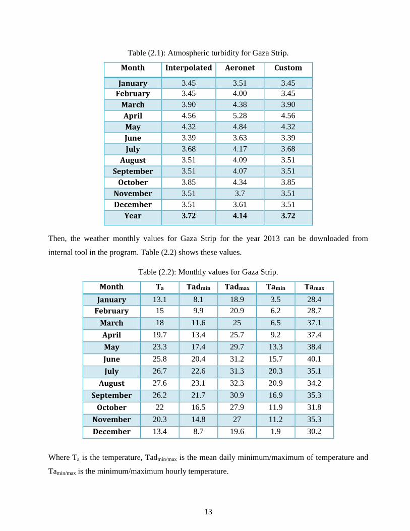


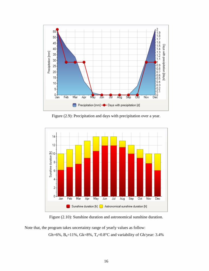
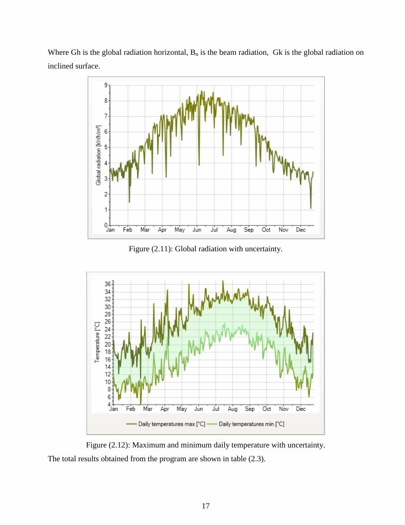


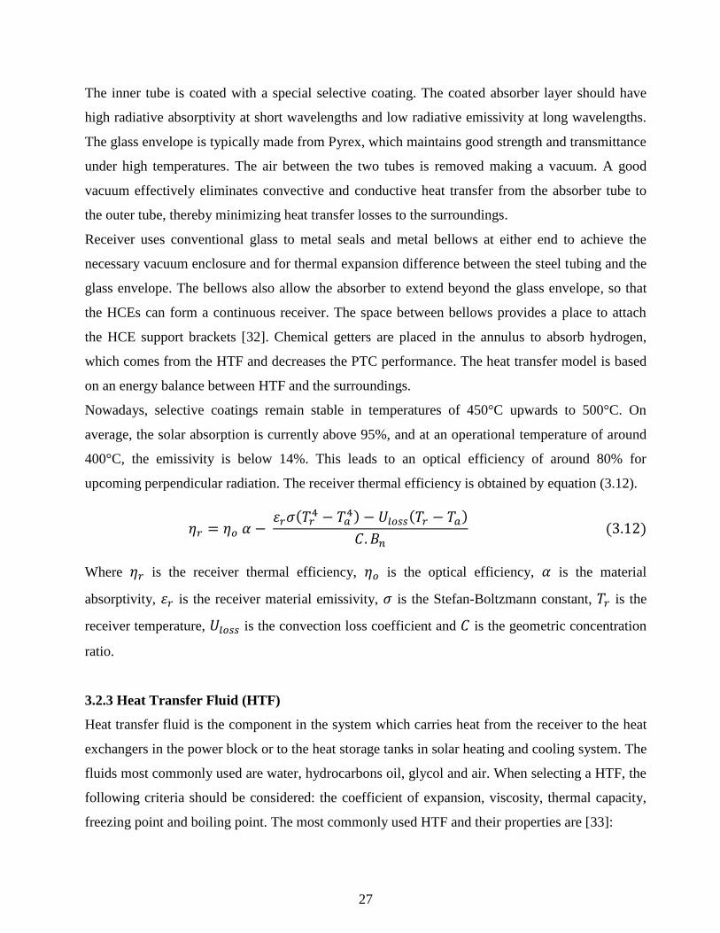


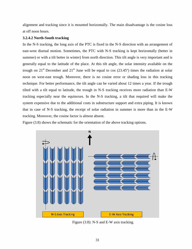


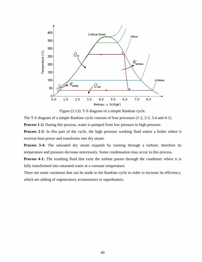


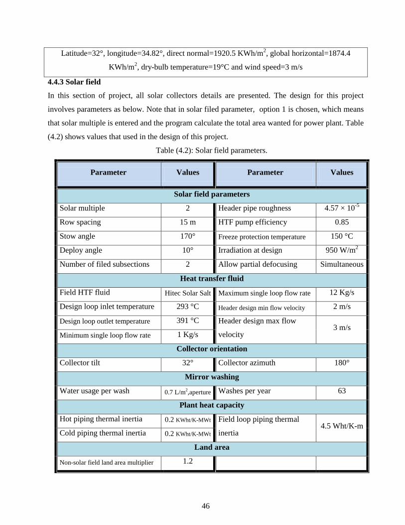


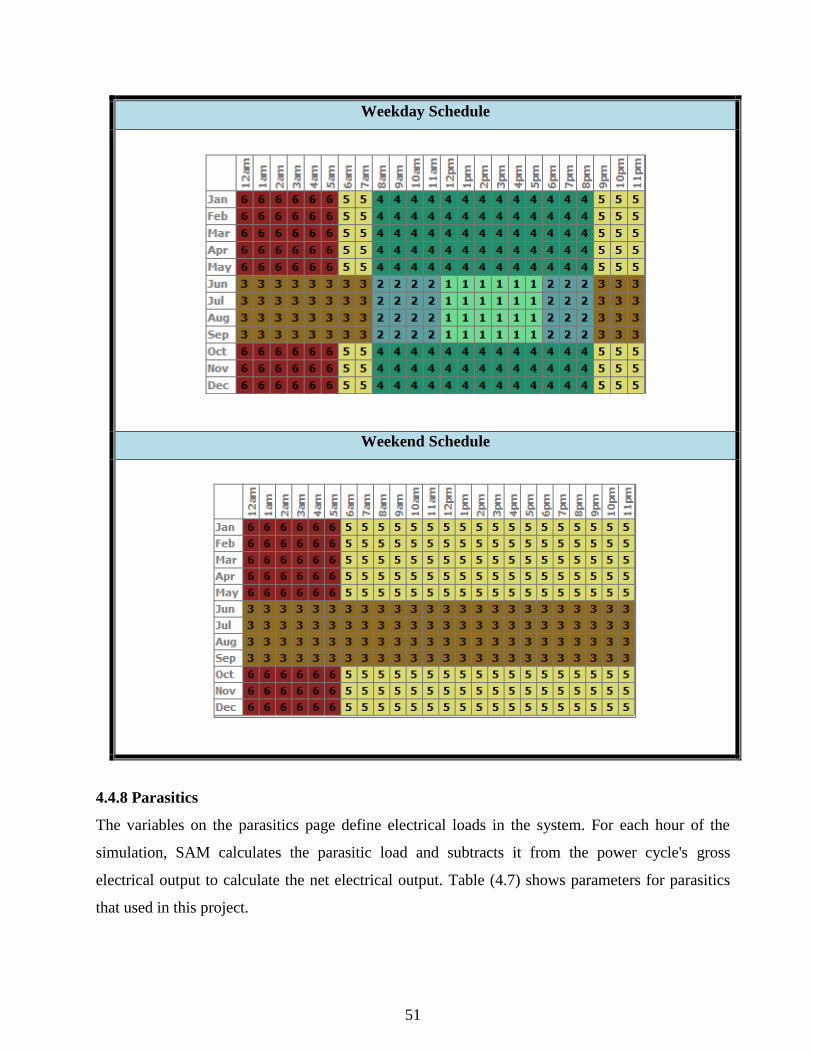

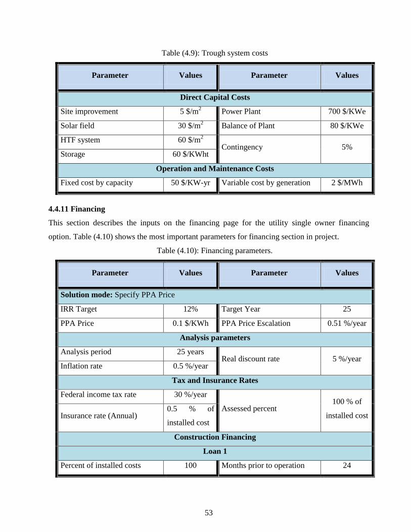


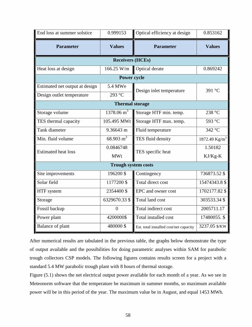


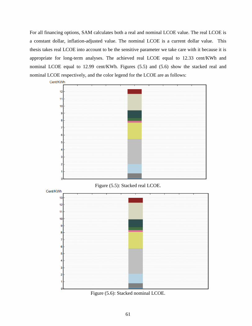
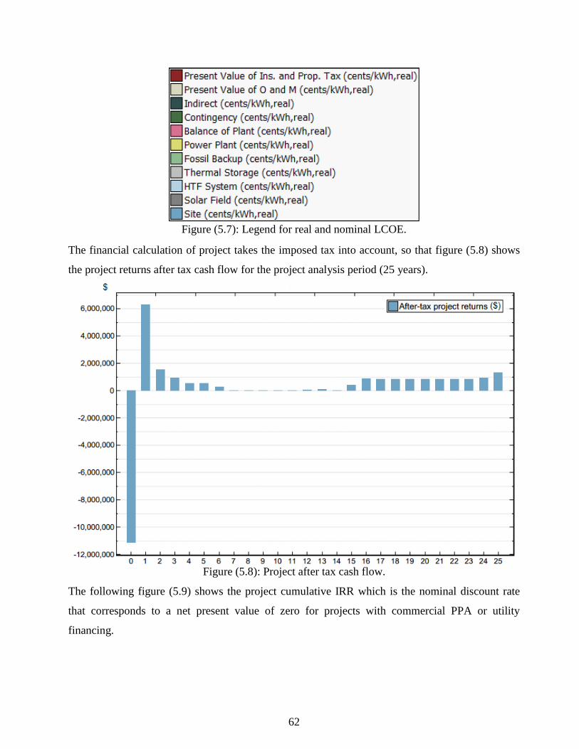
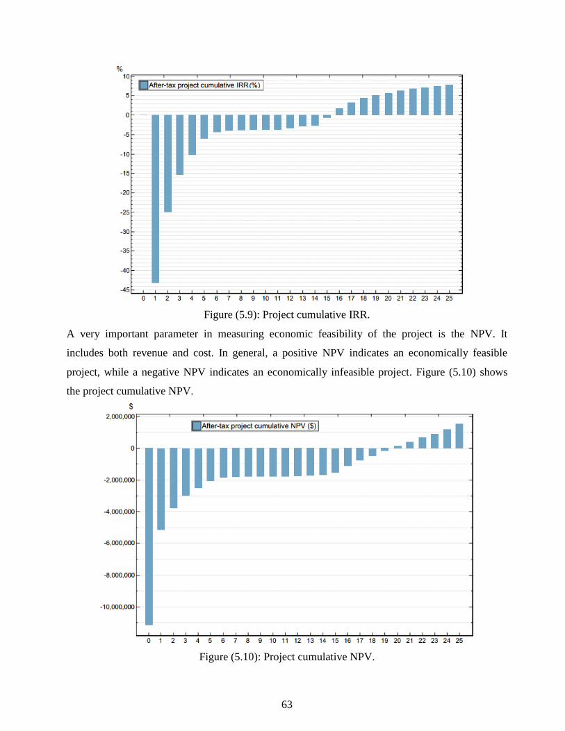


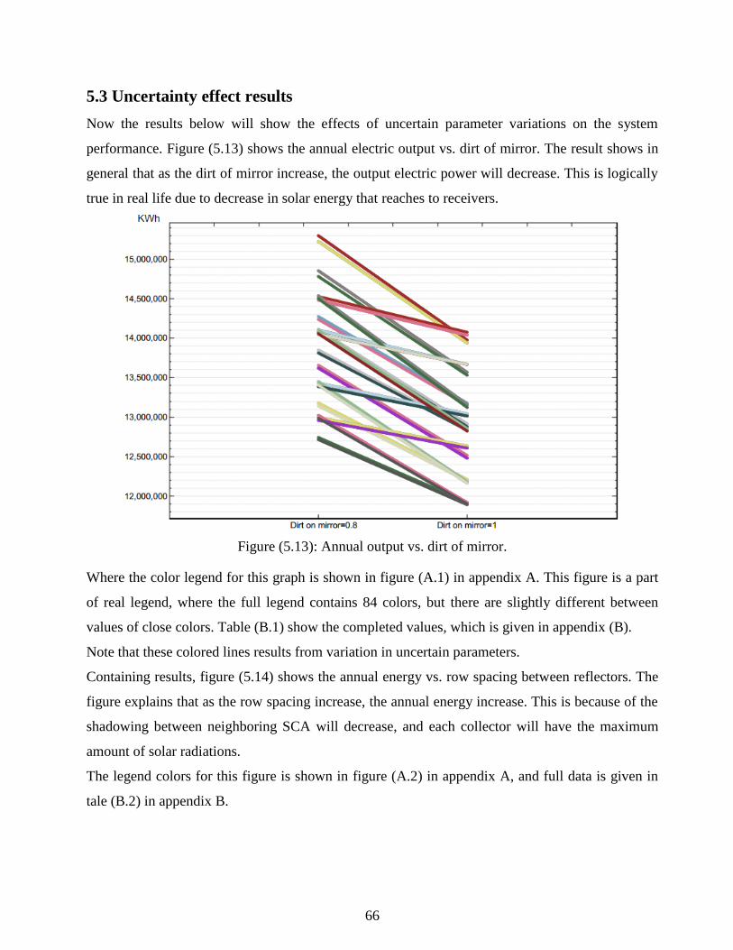


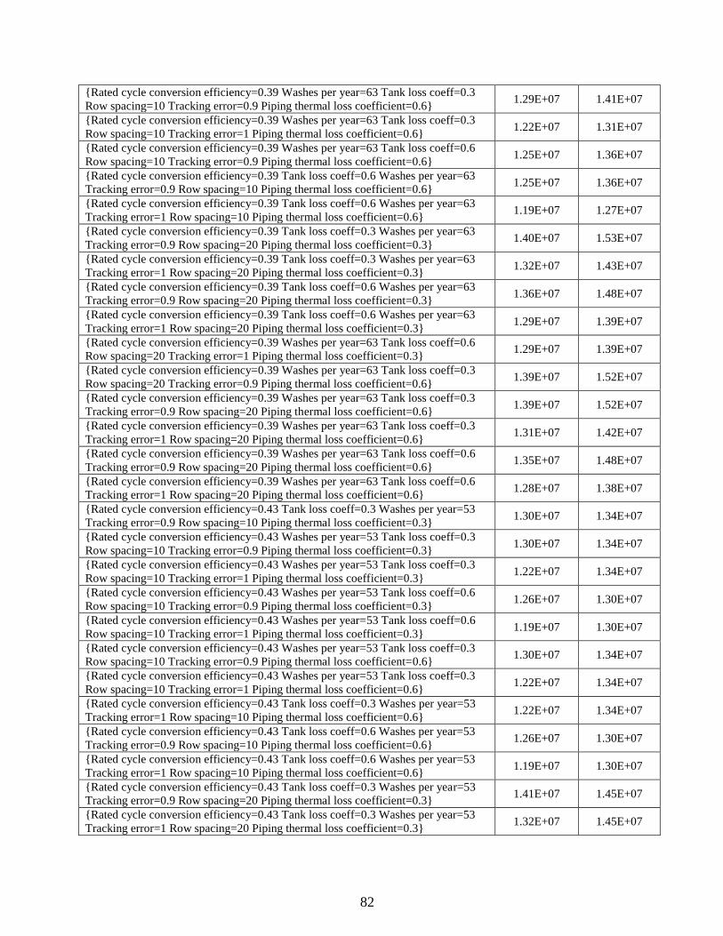
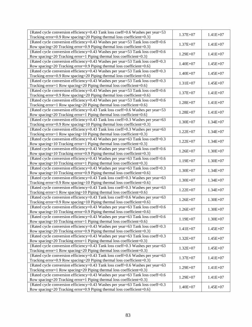
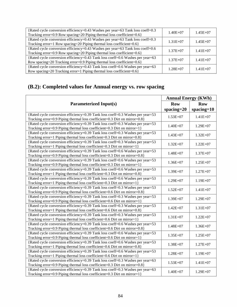

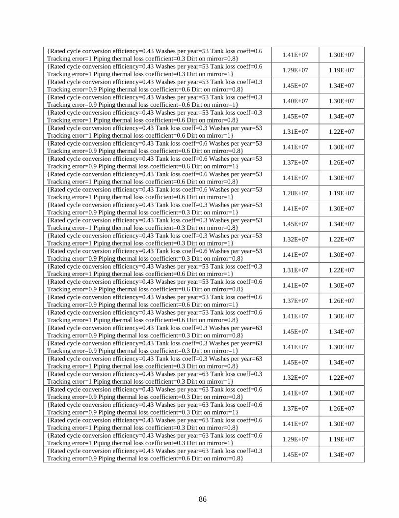

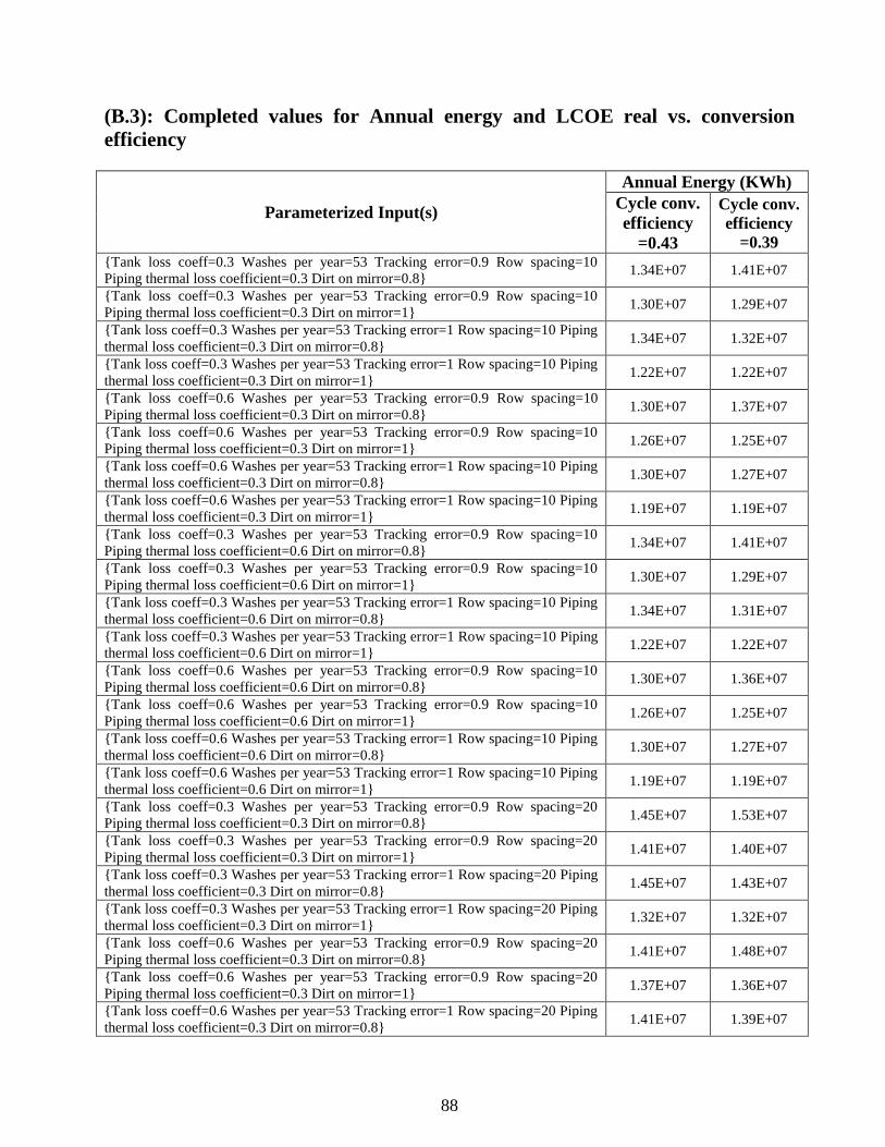

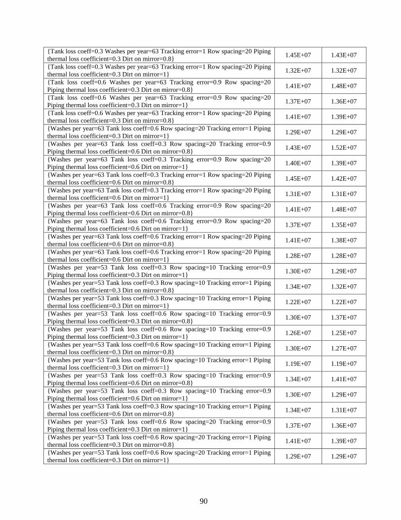


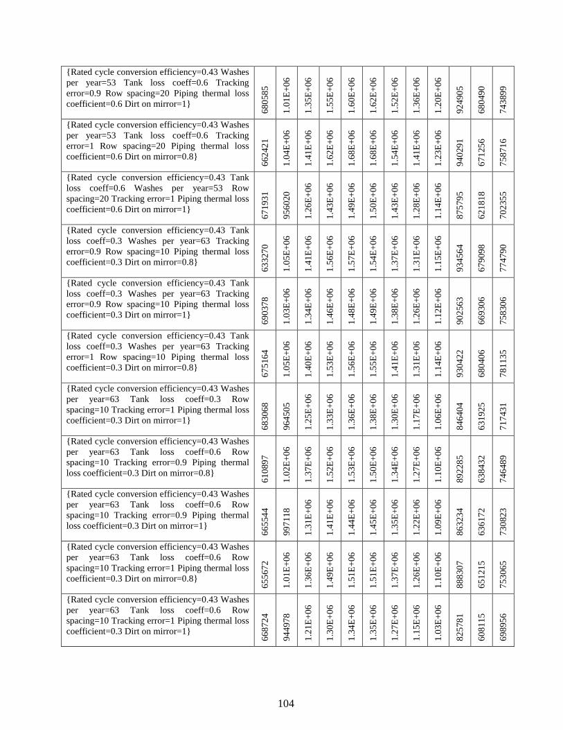


![Robust Model Predictive Control - Carnegie Mellon …cepac.cheme.cmu.edu/.../Ronust_Control_Classnotes.pdf1 Robust Model Predictive Control Formulations of robust control [1] The robust](https://static.documents.pub/doc/80x56/5aab45707f8b9a2b4c8bd345/robust-model-predictive-control-carnegie-mellon-cepacchemecmueduronustcontrol.jpg)


