Robust Estimates for GARCH Models By Nora Muler and Victor J. Yohai Universidad Torcuato Di Tella and Universidad de Buenos Aires and CONICET Abstract In this paper we present two robust estimates for GARCH(p,q) models. The first is defined by the minimization of a conveniently modified likelihood and the second is similarly defined, but includes an additional mechanism for restricting the propagation of the effect of one outlier on the next estimated conditional variances. We study the asymptotic properties of our estimates proving consistency and as- ymptotic normality . A Monte Carlo study shows that the quasi max- imum likelihood estimate practically collapses when there is a small percentage of outlier contamination, while the proposed robust esti- mates perform much better. This Monte Carlo study also includes two other robust estimates : a maximum likelihood estimate based on a Student distribution and the least absolute deviation estimate pro- posed by Peng and Yao. Moreover, we consider several real examples with financial data that illustrate the behavior of these estimates. Classification code: C22 Keywords: GARCH models, robust estimation, M-estimates, out- liers. 1 Introduction In a seminar paper, Engle (1982) introduced the autoregressive conditional heteroskedastic (ARCH) models. ARCH models were the first of a large fam- ily of heteroskedastic time series models such as, for example, the GARCH introduced in Bollerslev (1986), ARCH-M models by Engle, Lilien and Robins (1987) and EGARCH in Nelson (1991). These models are usually estimated by maximum likelihood assuming that the distribution of one observation conditionally to the past is normal. If the data satisfy the assumption of conditional normality, this procedure 1
Transcript
Robust Estimates for GARCH Models
By Nora Muler and Victor J. YohaiUniversidad Torcuato Di Tella
andUniversidad de Buenos Aires and CONICET
Abstract
In this paper we present two robust estimates for GARCH(p,q)models. The first is defined by the minimization of a convenientlymodified likelihood and the second is similarly defined, but includesan additional mechanism for restricting the propagation of the effectof one outlier on the next estimated conditional variances. We studythe asymptotic properties of our estimates proving consistency and as-ymptotic normality . A Monte Carlo study shows that the quasi max-imum likelihood estimate practically collapses when there is a smallpercentage of outlier contamination, while the proposed robust esti-mates perform much better. This Monte Carlo study also includestwo other robust estimates : a maximum likelihood estimate based ona Student distribution and the least absolute deviation estimate pro-posed by Peng and Yao. Moreover, we consider several real exampleswith financial data that illustrate the behavior of these estimates.Classification code: C22Keywords: GARCH models, robust estimation, M-estimates, out-liers.
1 Introduction
In a seminar paper, Engle (1982) introduced the autoregressive conditionalheteroskedastic (ARCH) models. ARCHmodels were the first of a large fam-ily of heteroskedastic time series models such as, for example, the GARCHintroduced in Bollerslev (1986), ARCH-M models by Engle, Lilien andRobins (1987) and EGARCH in Nelson (1991).
These models are usually estimated by maximum likelihood assumingthat the distribution of one observation conditionally to the past is normal.If the data satisfy the assumption of conditional normality, this procedure
1
is asymptotically efficient. Moreover, even when the conditional distribu-tion of the observations is not normal, these procedures give consistent andasymptotically normal estimates under certain moment conditions. The as-ymptotic properties of this estimate, known as quasi-maximum likelihood(QML) estimate, were studied by Lee and Hansen (1994) and Lumsdaine(1996) for the GARCH(1, 1) model. Elie and Jeantheau (1995) establishedstrong consistency of the QML-estimate in the GARCH (1, 1) model andBoussama (2000) proved the asymptotic normality of the same estimate.For the general GARCH(p, q) model, asymptotic properties of this estimatorwere studied for instance by Berkes, Hovath and Kokoszka (2003), Strau-mann and Mikosch (2003) and Christian and Zakoian (2004). These resultsshow that if the innovation has four moments, then the QML—estimate isconsistent and has asymptotically normal distribution. Hall and Yao (2003)show that if the fourth moment of the innovation is infinity, then the as-ymptotic distribution of the QML-estimate may not be normal.
These estimates based on a normal likelihood are very sensitive to thepresence of a few outliers in the sample. In fact, a single huge outlier mayhave a very large effect on the QML-estimate. Estimates that are not muchinfluenced by a small fraction of outliers are called robust estimates.
Several types of outliers have been studied for time series such as additiveoutliers and innovation outliers. Outliers may be isolated or occur in patches.In our simulated studies we consider only isolated additive outliers. Theseoutliers can be modeled as follows. Suppose that the GARCH(p, q) series isgiven by xt. Then, the observed series corresponding to the isolated additiveoutliers is
xt + vtut,
where xt, vt and ut are independent processes. Here vt, and ut are sequencesofindependent and identically distributed (i.i.d.) random variables and thevariable ut takes values 0 and 1. The event ut = 1 indicates that an outlieroccurs at time t, and therefore xt + vt is observed instead of xt. Usuallyθ = P (ut = 1) is small, so that most of the time the GARCH series xt isobserved. Mendes (2000) studied the asymptotic bias produced by additiveoutliers on the QML-estimate.
Several authors have proposed robust estimates for ARCHmodels. Sakataand White (1998) proposed estimates based on an M-scale, Mendes andDuarte (1999) defined a class of constrained M-estimates and Muler andYohai (2002) introduced a class of estimates based on a τ−scale estimate
2
combined with robust filtering. Jiang, Zhao and Hui (2001) proposed L1estimates of modified ARCH models. Franses and van Dijk ( 2000) andCarnero, Pena and Ruiz (2001) used diagnostic procedure for detecting out-liers in GARCH models. Rieder, Ruckdeschel and Kohl (2002) introduced aclass of robust estimates for a general class of models that includes GARCH,based on the minimization of the mean square error on infinitesimal neigh-borhoods of contamination. Robust tests for ARCH heteroskedasticity wereproposed by van Dijk, Lucas and Franses (1999) and Ronchetti and Trojani(2001).
Li and Kao (2002) proposed a bounded influence estimate for a logGARCH (1,1) model introduced by Geweke (1986). Park (2002) consid-ered a modified GARCH model where the conditional standard deviation(instead of the variances as in GARCH) is modelled as a linear combinationof the preceding standard deviations of the absolute values of the precedingobservations. The proposed estimator is based on a least absolute deviation(LAD) criterion. Peng and Yao (2003) propose estimates for the GARCHmodel which are also variations of the LAD criterion. Finally a widespreadprocedure of protection against heavy tailed distributions in GARCHmodelsuses a maximum likelihood estimate assuming that the conditional distrib-ution given the past is a heavy tailed distribution (like a Stude nt with asmall degree of freedom) instead of the normal distribution.
Huber (1981) considers a stricter concept for a robust estimate. It shouldsatisfy the following two properties:
(H1) The estimate should be highly efficient when all observations ofthe sample follow the assumed model. This condition can be checked bycomparing its efficiency to that of the maximum likelihood estimate for thatmodel.
(H2) Replacing a small fraction of observations of the sample by outliersshould produce a small change in the estimate. This property was formal-ized in terms of continuity of the estimate and called qualitative robustnessby Hampel (1971) for independent observations. Boente, Fraiman and Yohai(1987) generalized this concept for time series.
None of the estimates mentioned above for the GARCH model simulta-neously satisfies H1 and H2. If the assumed model is a GARCH model withnormal conditional distribution, neither the maximum likelihood estimatescorresponding to a heavy tailed distribution nor those based on a LAD cri-terion satisfy the property H1 stated above. This is shown in Table 1 ofSection 4 where we compute the efficiencies of some of these estimate forthe normal GARCH. Although these estimators behave much better than
3
the QML-estimate when the conditional distribution has heavy tailed dis-tributions, they also fail to satisfy property H2. See Section 4 where wereport of the results of a Monte Carlo study, showing that a small fractionof additive outliers may have a large influence on them.
In this paper we present two classes of robust estimates for GARCHmod-els. The first class can be considered an extension of the M-estimates intro-duced by Huber (1964) for location and Huber (1973) for regression. Theyare obtained by maximizing a conveniently modified likelihood function.We show that the M-estimates are consistent and asymptotically normal.These M-estimates are less sensitive to outliers than the QML-estimate andsatisfy H1 However they do not satisfy criterion H2, i.e., a few large outlierscan still have a large influence on them. This lack of robustness is due to thefact that a single large outlier may have much influence on the conditionalvariance of an undetermined large number of subsequent observations.
To improve robustness, we propose another estimate that includes anadditional mechanism that restricts the propagation of the outlier effect insuch a way that the influence of past variances on the present observation arebounded. These estimates are called bounded M-estimates (BM-estimates).BM-estimates are also consistent and asymptotically normal and they pos-sess both properties H1 and H2, i.e., they have a high efficiency under aGARCH normal model and are not much influenced by a small fraction ofoutlying observations.
In financial data it is very common to use GARCH models to predictstock volatilities, which are one of the parameters required to determine op-tion prices It may be argued that since outlying observations really happenand represent a risk factor, they should be taken into account to determinethe option prices. This line of thinking would conclude that for these appli-cations the QML-estimates for GARCH models, which does not downweightthe effect of outliers, may be preferable to robust estimates. The followingthree comments respond to this criticism:
(i) A model with robustly estimated parameters fits the majority of theobservations. Instead, if the data contains gross departures from the model,the QML-estimate may fit the bulk of the data poorly while fitting some ofthe outliers.
(ii) When a robust estimate is used, outliers can be detected as obser-vations not well fitted by the estimated model. This allows the possibilityto improve the model by including variables that explain the outliers. How-ever, if a non robust estimate is used, the outliers may remain hidden, thusprecluding the possibility of improving the model.
4
(iii) The downweighting of outliers in the robust estimation process doesnot preclude their use in prediction, since the estimated coefficients deter-mine only the predictive dynamics of the model. If the recent past containsoutliers and the user assumes that these outliers are valid inputs for predic-tion, they may be used as such without downweighting.
This paper is organized as follows. In Section 2, we state some of theproperties of GARCH processes and define the proposed robust estimates.In Section 3, we give the consistency and asymptotically normality results.In Section 4, we report the results of a Monte Carlo Study for the QML-estimate, the Peng and Yao LAD estimator, the maximum likelihood es-timates corresponding to a Student distribution with a small degrees offreedom (SML) and our proposed M- and BM-estimators. These resultsshow a clear advantage of the robust estimates when the sample containsoutliers, especially in the case of the BM-estimate. In Section 5, we considerexamples of series corresponding to daily data and compare the truncatedvariance and rank correlation of the errors for the daily returns series of theQML-estimate, the LAD-estimate, the SML- and the BM-estimate. Section6 contains some concluding remarks. Section 7 is an Appendix with someof the proofs. For brevity sake we omit several proofs which can be foundin a technical report by Muler and Yohai (2005).
2 Robust Estimates for GARCH(p, q) Models
A series x1, ..., xT is a centered GARCH (p, q) process if
xt = σtzt, (1)
where z1, z2, ..., zT are i.i.d. random variables with a continuous density fsuch that E(zt) = 0 and var(zt) = 1(var(x) denotes variance of x) and wherethe conditional variances σ2t are given by
σ2t = α0 +pXi=1
αix2t−i +
qXi=1
βiσ2t−i,
where αi ≥ 0, 1 ≤ i ≤ p, βi ≥ 0, 1 ≤ i ≤ q and α0 > 0. We denoteα = (α0,α1, ...,αp), β = (β1, ...,βq) and γ = (α,β). When q = 0 we obtainthe class of ARCH models introduced by Engle (1982).
A necessary and sufficient condition for strict stationarity of the processxt with finite variance is
Σpi=1αi +Σqi=1βi < 1, (2)
5
see Bollerslev (1986), Nelson (1990), Bougerol and Picard (1992) and Gi-raitis, Kokoszka and Leipus (2000). In this case
var(xt) =α0
1− (Ppi=1 αi +
Pqi=1 βi)
. (3)
The following condition is required for identification of the GARCH pa-rameters.
A(x) = Σpi=1αixi and B(x) = 1− Σqi=1βixi are coprimes. (4)
Hall and Yao (2003) show that an explicit form for σ2t is
σ2t =α0
1−Pqi=1 βi
+pXi=1
αix2t−i+
pXi=1
αi
∞Xk=1
qXji=1
· · ·qX
jk=1
βj1 · · ·βjkx2t−i−j1−···−jk .
(5)Put yt = log(x
2t ) and wt = log(z
2t ). Then we have
yt = wt + log σ2t .
If the density f of zt is symmetric around 0, then the density of wt is ggiven by
g(w) = f(ew/2)ew/2. (6)
In particular when f corresponds to the N(0,1) distribution, g = g0 where
g0(w) =1√2πe−
12(ew−w). (7)
Given the parameter values c = (a,b) where a = (a0, a1, ..., ap),b =(b1, ..., bq) we define for all t
ht(c) = a0 +pXi=1
aix2t−i +
qXi=1
biht−i(c). (8)
where xt = 0 for t ≤ 0 and so
ht(c) =a0
1−Pqi=1 bi
6
for all t ≤ 0. From (5) we obtain that
ht(c) =a0
1−Pqi=1 bi
+pXi=1
aix2t−i
+pXi=1
ai
∞Xk=1
qXji=1
· · ·qX
jk=1
bj1 · · · bjkx2t−i−j1−···−jk It−i−j1−···jk≥1.
These initial conditions are the same as those used by Hall and Yao (2003).The usual form of the QML-estimate based on the xt’s consists on max-
imizing
−12
TXt=p+1
x2tht(c)
− 12
TXt=p+1
loght(c) (9)
and since yt = log(x2t ), this can be written as
−12
TXt=p+1
³eyt−log ht(c) + log ht(c)
´.
Then, to maximize (9) is equivalent to maximize
L0,T (c) =TX
t=p+1
log(g0(yt − log ht(c)). (10)
where the function g0 is given by (7).Observe that this equivalence does not require that the true density f
of zt be symmetric.Maximizing (10) is equivalent to minimizing
M0,T (c) =1
T − pTX
t=p+1
ρ0(yt − log ht(c)), (11)
whereρ0 = − log(g0), (12)
where g0 is given in (7).In a similar way, it can be proved that the ML-estimate for a GARCH(p, q)
model corresponding to any symmetric density f∗ (it is not necessary thatf∗ coincides with the true density f) is obtained by minimizing
1
T − pTX
t=p+1
ρ∗(yt − log ht(c)),
7
where ρ∗ = − log(g∗) and g∗ is given by (6) with f = f∗.As could be expected, the QML-estimate is not robust, i.e., a few outliers
may have a large influence on this estimate. This can be seen in our MonteCarlo simulation in Section 4. One reason for the lack of robustness of theQML-estimate is that ρ0 is unbounded, so that one large outlier may havean unbounded effect on M0,T .
Put
MT (c) =1
T − pTX
t=p+1
ρ(yt − loght(c)). (13)
Then, the M-estimates for GARCH models are defined as
bγ = argminc∈C
MT (c) (14)
for some convenient compact set C. These estimates can be considered ageneralization of the class of M-estimates proposed by Huber (1964) forlocation and Huber (1973) for regression.
DefineJ(u) = E(ρ(wt − u)).
In Lemma 1 we show that J(u) is well defined when ρ0 is finite.Lemma 1. Consider a stationary GARCH model xt given by (1). Then(a) E(|wt|) <∞ and (b) If ψ = ρ0 is finite, then J(u) is finite for all u.To guarantee good consistency properties of the estimates we need that
ρ satisfy the following propertyP1. There exists a unique value u0 where J(u) takes the minimum.Bollerslev, Chou and Kroner (1992) proposed using the ML-estimate
for zt having a symmetric heavy tail distribution, for example a Studentdistribution with a small degree of freedom. This corresponds to an M-estimate with ρ = − log(g), where g is the density of log(z2). Peng and Yao(2003) LAD estimate corresponds to ρ(u) = |u|.
We can distinguish two types of M-estimates: (i) M-estimates with ρ0
bounded but ρ unbounded (ii) M-estimates with both ρ and ρ0 bounded.The M- estimates with ρ0 bounded but ρ unbounded are robust when zthas heavy tail distribution, although they may be much affected by anothertype of outliers as for example additive outliers, as we see in our MonteCarlo simulation in Section 4. To increase the degree of robustness we needthat ρ be bounded too. There is extensive literature on the properties of M-estimates for regression. For example, Huber (1973) shows that M-estimatesfor regression with bounded ρ0 are robust when the distribution of the error
8
is heavy tailed. Yohai (1987) shows that M-estimates for regression with ρbounded are robust against any kind of outliers.
The ML-estimates for heavy tail zt and the Peng and Yao (2003) LADestimates are examples of M-estimates with bounded ρ0 but unbounded ρ.For instance for the Student distribution with three degrees of freedom wehave
ρ(u) = 2 ln (1 + eu)− u/2and
ρ0(u) =3eu − 12(1 + eu)
.
For the Peng and Yao estimate we have
ρ(u) = |u|, ρ0(u) = sign(u).
M-estimates with ρ bounded are more robust than the QML-estimate,although large outliers may still have a strong effect on the estimates. Thereason is that this estimate requires computing the values ht(c) using (8),so a large outlier at time t may affect all the ht0(c) with t
0 > t.The same problem appears in the estimates of ARMA models, where
an outlier at time t may influence the estimated innovations correspondingto several periods. To deal with this problem, several authors used ro-bust filters. See Denby and Martin (1979), Martin, Samarov and Vandaele(1983) and Bianco, Garcia Ben, Martinez and Yohai (1996). Muler andYohai (2002) used robust filters for estimating ARCH models. However, theasymptotic theory of these estimates is very complicated and proofs of as-ymptotic normality are not available.
In this paper we propose a method related to robust filters, which hasthe advantage that the resulting estimates are mathematically tractable. Togain robustness, we modify the M-estimates for GARCHmodels by includinga mechanism which restricts the propagation of the outlier effect on theestimated ht(c)’s. For this purpose, we replace in the computation of theM-estimate ht(c) by
h∗t,k(c) = a0 +pXi=1
aih∗t−i,k(c)rk
Ãx2t−i
h∗t−i,k(c)
!
+qXi=1
bih∗t−i,k(c), (15)
9
where xt = 0 for t ≤ 0 and where
rk(u) =
(u if u ≤ kk if u > k.
. (16)
Observe that if k is large, then ht(c) and h∗t,k(c) are close. However
the propagation of the effect of one outlier in time t on the h∗t0,k(c), t0 > t,
practically vanishes after a few periods. Therefore, if xt follows a GARCHmodel but contains some outliers, we may expect that the M-estimates usingconditional variances given by (15) would fit better than the M-estimate cor-responding to the GARCH model. This suggests modifying the M-estimateas follows. Let bγ1 be defined as in (14) and bγ2 by
bγ2 = argminc∈C
M∗Tk(c), (17)
where
M∗Tk(c) =
1
T − pTX
t=p+1
ρ(yt − log h∗t,k(c)). (18)
When the process is a perfectly observed GARCH process without out-liers the conditional variances are given by (8). Then the estimate bγ1usingthese conditional variances generally behaves better than bγ2. In this case bγ2is asymptotically biased and we may expect MT (bγ1) ≤M∗
Tk(bγ2). Theorem4 of Section 3 proves that this holds asymptotically with probability one.As explained above, when there are outliers, bγ2 may be preferable and wemay expect MT (bγ1) > M∗
Tk(bγ2). Then we define the BM-estimate byγB =
( bγ1 if MT (bγ1) ≤M∗Tk(bγ2)bγ2 if MT (bγ1) > M∗Tk(bγ2). (19)
We will see that BM-estimates simultaneously possess both properties:robustness against outliers and consistency when the series follows a GARCHmodel without outliers. Moreover, by choosing m and k conveniently, theseestimates have high efficiency under the GARCH model
Our proposal is to use BM-estimates with ρ of the form ρ = m(ρ0),where m is a bounded nondecreasing function. We see in the next sectionthat this function satisfies P1 with u0 = 0 when zt is normal. Moreover, asshown in Section 4, when we take m equal to the identity in a sufficientlylarge interval, the BM-estimates are going to be highly efficient when zthas normal distribution and less sensitive to additive outliers than the otherestimates mentioned in this section.
10
However, if we consider that zt has a symmetric density f different fromthe normal, it is possible to define ρ = m(− log(g)) where g is given by (6)and ρ is a non decreasing and bounded function.
3 Asymptotic results
In this Section we state the main asymptotic results for the M- and BM-estimates: consistency and asymptotic normality. In Theorems 1, 2 and 3 weprove the consistency and asymptotic normality for any M-estimate definedin (14) as long as P1 holds and ρ0 is bounded. In Theorem 4 and 5 we provethe consistency and asymptotic normality for the proposed BM-estimators.
Suppose first that we have the infinite sequence of observations Xt =(..., xt−1, xt) corresponding to a GARCH(p, q) process up to time t with pa-rameter γ = (α,β), and given c = (a,b) call eht(c) the conditional varianceof xt given Xt−1 when γ = c. Then the following recursive relationship issatisfied
eht(c) = a0 + pXi=1
aix2t−i +
qXi=1
bieht−i(c). (20)
The following Theorem shows the Fisher consistency of the M-estimatesof the GARCH model and gives a sufficient condition for P1.
Denote by
Rn+ = {x = (x1, ...xn) : xi ≥ 0, 1 ≤ i ≤ n}.Theorem 1. Let xt be a stationary GARCH(p, q) process satisfying (1)
and (2). Let yt = log(x2t ) and define for c = (a,b) ∈ Rp+q+1+
M(c) = E(ρ(yt − eht(c)).Suppose that ρ0 is bounded, that P1 and (4) hold and that βq > 0 in
the case of a GARCH(p,q) process or αp > 0 in the case of an ARCH(p)process. Then
(i) M(c) is minimized when ai = eu0αi, 0 ≤ i ≤ p, bi = βi, 1 ≤ i ≤ q.
(ii) Assume that wt = log(z2t ) has a density g(w) that is unimodal, contin-
uous and positive for all w. If we take ρ = m(− log(g)), where m ismonotone, P1 holds with u0 = 0.
11
Observe that according to part (i) of Theorem 1, the M-estimate of αshould be corrected by the factor e−u0 for consistency. Part (ii) shows that ifwe take ρ = m(− log(g)) there is no need of correction. An alternative thatavoids the correction factor is to replace ρ(u) with ρ(u) = ρ(u − u0), andthen in the rest of the paper without loss of generality we assume u0 = 0.
Put
Cδ =
((a,b) : a ∈Rp+1+ , b ∈Rq+, a0 ∈ [δ, 1/δ],
pXi=1
ai ≥ δ ,
pXi=1
ai +qXj=1
bj ≤ 1− δ
(21)
The set C in (14) and (17) is taken as Cδ0 for some δ0 > 0.Put γ = (α0,α1, ...αp,β1, ...,βq). The following two Theorems state the
consistency and asymptotic normality of the M-estimates to γ.Theorem 2. Suppose that all the assumptions of Theorem 1 hold. Let bγTbe defined as in (14) with C = Cδ0 given by (21). We also assume that P1 issatisfied with u0 = 0, that ρ has a bounded derivative, and that γ ∈C. ThenbγT → γ a.s..Theorem 3. Suppose that all the assumptions of Theorem 2 hold. As-sume also that (i) ρ has three continuous and bounded derivatives, (ii)E(ψ2(wt)) > 0 and (iii) E(ψ
0(wt)) > 0, where ψ = ρ0. Then T 1/2(bγT − γ)converges in distribution to a N(0, V ) and
V =Eg(ψ
2(wt))
E2g(ψ0(wt))
ÃEg
Ã1eh2t (γ)∇eht(γ)∇eht(γ)0
!!−1, (22)
where ∇h denotes gradient of h.For the case of the QML-estimate, we have ρ = ρ0 given in (12). Then
the assumption of ρ0 bounded is not satisfied. However, in the case thatzt has a finite fourth moment, the QML-estimate has asymptotic normaldistribution with a covariance matrix given by (22). See Berkes, Hovath andKokoszka (2003). Then the relative asymptotic efficiency of the M-estimatewith respect to the QML-estimate is given by
AEF =a(ψ, g)
a(ψ0, g),
where ψ0 = ρ00 and
12
a(ψ, g) =Eg(ψ
2(wt))
E2g (ψ0(wt))
.
Therefore, by choosing m bounded and close to the identity function, wecan obtain a robust estimate that is highly efficient when the zt’s are normal.
The next two Theorems show that asymptotically the M and BM-estimatesare equivalent when xt follows an exact GARCH model without outliers.Theorem 4. Suppose that all the assumptions of Theorem 3 hold and thatthe distribution of zt gives positive probability to the complement of anycompact. We also assume that lim|u|→∞ ρ(u) = supu ρ(u). Moreover if we
let bγT be the M-estimate defined by (14) and γBT the BM-estimate definedby (19), then limT→∞ P (γBT = bγT ) = 1.
Remark. Suppose that g is a unimodal and positive density. Then, itcan be proved that the assumption lim|u|→∞ ρ(u) = supu ρ(u) holds if wetake ρ = m(− log(g)) and m non decreasing.
From Theorems 2, 3 and 4 we derive the following result.Theorem 5. Theorems 2 and 3 also hold for the BM-estimate γBT .
4 Monte Carlo Simulation
We performed a Monte Carlo study to compare the behavior of seven es-timates: (i) the QML-estimate (QML), (ii) the maximum likelihood cor-responding to zt with Student distribution with three degrees of freedom(SML) (iii) the LAD Peng-Yao estimate (LAD), (iv) the M-estimate basedon a loss function ρ1 = m1(ρ0), where ρ0 is given in (12) and m1 is a nonde-creasing, bounded and close to the identity function which is defined below(M1), (v) A BM-estimate as defined in (19) with ρ = ρ1 and k = 5.02 (BM1),(vi) an M-estimate based on a loss function ρ2 defined as ρ2(x) = m2(ρ0(x)),m2(v) = 0.8m1(v/0.8) (M2) and (vii) A BM-estimate as defined in (19) withρ = ρ2 and k = 3 (BM2).
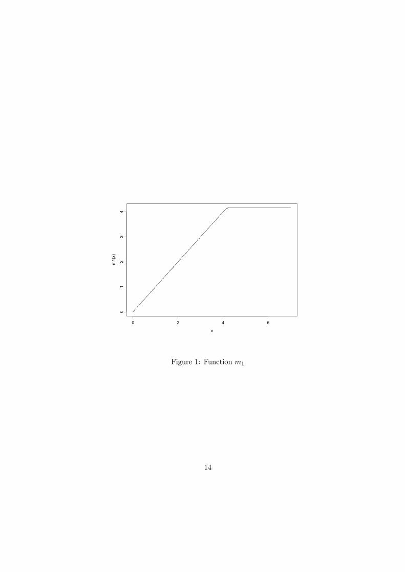
The function m1 is defined as
m1(x) =
x if x ≤ 4. 02c4x
4 + c3x3 + c2x
2 + c1x+ c0 if 4. 02 < x ≤ 4. 304.16 if x > 4. 30,
where c0 = 6777, c1 = −6536.2, c2 = 2362.3, c3 = −379.0087, c4 = 22.7770.This function is shown in Figure 1.
13
x
m1(
x)
0 2 4 6
01
23
4
Figure 1: Function m1
14
As we see in Figure 1, m1 is a smoothed version of
m (x) =
(x if x ≤ 4.024.02 if x > 4.02.
The function m1 is equal to the identity in a larger interval than m2and therefore the estimates based on m1 are more similar to the QML thanthose based on m2. These, (see in Table 1), make estimates M1 and BM1
more efficient than estimates M2 and BM2. As a counterpart we see in ourMonte Carlo results that the first estimates are going to be less robust thanthe second ones. The choice of m1 and m2 were done so
P (ρ1(wt) = ρ0(wt)) = 0.96. (23)
andP (ρ2(wt) = ρ0(wt)) = 0.90
when wt is log(z2t ) and zt is N(0,1).
After several trials, the value of k in (16) for BM1 was taken as equal to5.02. This value is such P (z2t ≤ 5.02) = 0.975, when zt is N(0,1). For theBM2 estimate, in order to gain robustness, we chose k = 2.72. This valueis such P (z2t ≤ 2.72) = 0. 90. We found in the Monte Carlo simulationsthat BM1 was a convenient trade off between efficiency under a normalGARCH model and robustness. Instead, BM2 has rather low efficiencyunder a GARCH model, but we found in the Monte Carlo simulation thatis more robust when the fraction of outliers is 10%.
The correction term u0 defined in P1 when zt is N(0,1) is 0.636 for theSML estimate and −0.787 for the LAD estimate. For the other estimatesit is zero. The asymptotic efficiencies (EFF) of all the estimates we usedin these simulations under a normal GARCH model are shown in Table1. We observe that the asymptotic efficiencies of the M1, BM1 and SMLestimates are quite high, the asymptotic efficiencies of M2 and BM2 areintermediate and the asymptotic efficiency of the LAD estimate is quitelow.Table 1. Asymptotic efficiencies (EFF) of the estimates under normalGARCH models.
Table 1. Asymptotic efficiencies (EFF) of the estimates under normalGARCH models.
Estimate QML SML LAD M1 and BM1 M2 and BM2
EFF 1 0. 79 0. 37 0. 83 0. 67
15
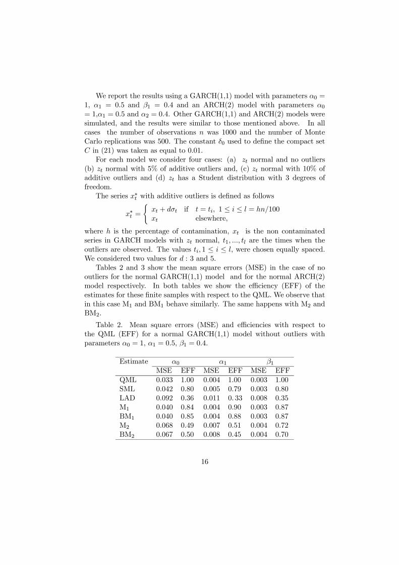
We report the results using a GARCH(1,1) model with parameters α0 =1, α1 = 0.5 and β1 = 0.4 and an ARCH(2) model with parameters α0= 1,α1 = 0.5 and α2 = 0.4. Other GARCH(1,1) and ARCH(2) models weresimulated, and the results were similar to those mentioned above. In allcases the number of observations n was 1000 and the number of MonteCarlo replications was 500. The constant δ0 used to define the compact setC in (21) was taken as equal to 0.01.
For each model we consider four cases: (a) zt normal and no outliers(b) zt normal with 5% of additive outliers and, (c) zt normal with 10% ofadditive outliers and (d) zt has a Student distribution with 3 degrees offreedom.
The series x∗t with additive outliers is defined as follows
x∗t =(xt + dσt if t = ti, 1 ≤ i ≤ l = hn/100xt elsewhere,
where h is the percentage of contamination, xt is the non contaminatedseries in GARCH models with zt normal, t1, ..., tl are the times when theoutliers are observed. The values ti, 1 ≤ i ≤ l, were chosen equally spaced.We considered two values for d : 3 and 5.
Tables 2 and 3 show the mean square errors (MSE) in the case of nooutliers for the normal GARCH(1,1) model and for the normal ARCH(2)model respectively. In both tables we show the efficiency (EFF) of theestimates for these finite samples with respect to the QML. We observe thatin this case M1 and BM1 behave similarly. The same happens with M2 andBM2.
Table 2. Mean square errors (MSE) and efficiencies with respect tothe QML (EFF) for a normal GARCH(1,1) model without outliers withparameters α0 = 1, α1 = 0.5, β1 = 0.4.
Table 3. Mean square errors (MSE) and efficiencies with respect to theQML (EFF) for a normal ARCH(2) model without outliers and parametersα0 = 1, α1 = 0.5, α2 = 0.4.
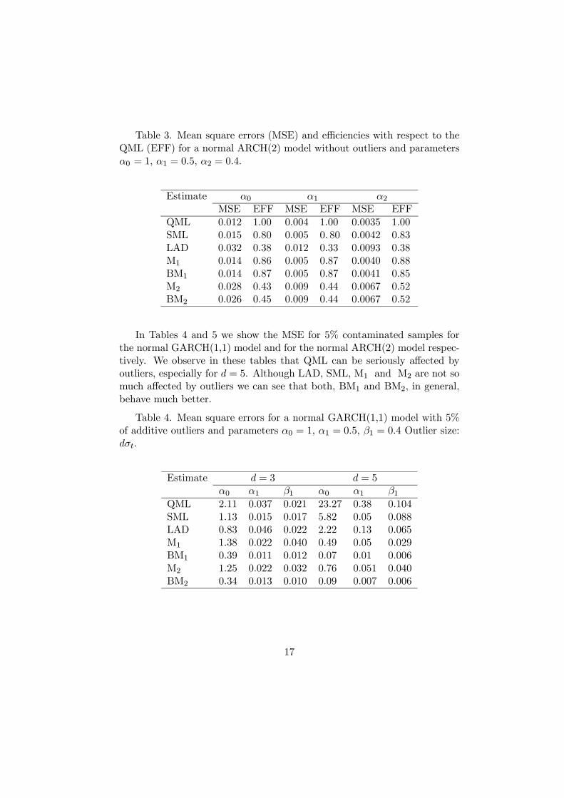
In Tables 4 and 5 we show the MSE for 5% contaminated samples forthe normal GARCH(1,1) model and for the normal ARCH(2) model respec-tively. We observe in these tables that QML can be seriously affected byoutliers, especially for d = 5. Although LAD, SML, M1 and M2 are not somuch affected by outliers we can see that both, BM1 and BM2, in general,behave much better.
Table 4. Mean square errors for a normal GARCH(1,1) model with 5%of additive outliers and parameters α0 = 1, α1 = 0.5, β1 = 0.4 Outlier size:dσt.
In Tables 6 and 7 we report the MSE for the normal GARCH(1,1) andnormal ARCH(2) models respectively when there is 10% outlier contamina-tion. In the case of d = 5 the behavior of the estimates is similar to the casewith 5% of outliers. In the case of d = 3 the only estimate that is not muchaffected by outliers is BM2.
Table 6 Mean square errors for a normal GARCH(1,1) model with 10%of additive outliers and parameters α0 = 1, α1 = 0.5, β1 = 0.4 Outlier size:dσt.
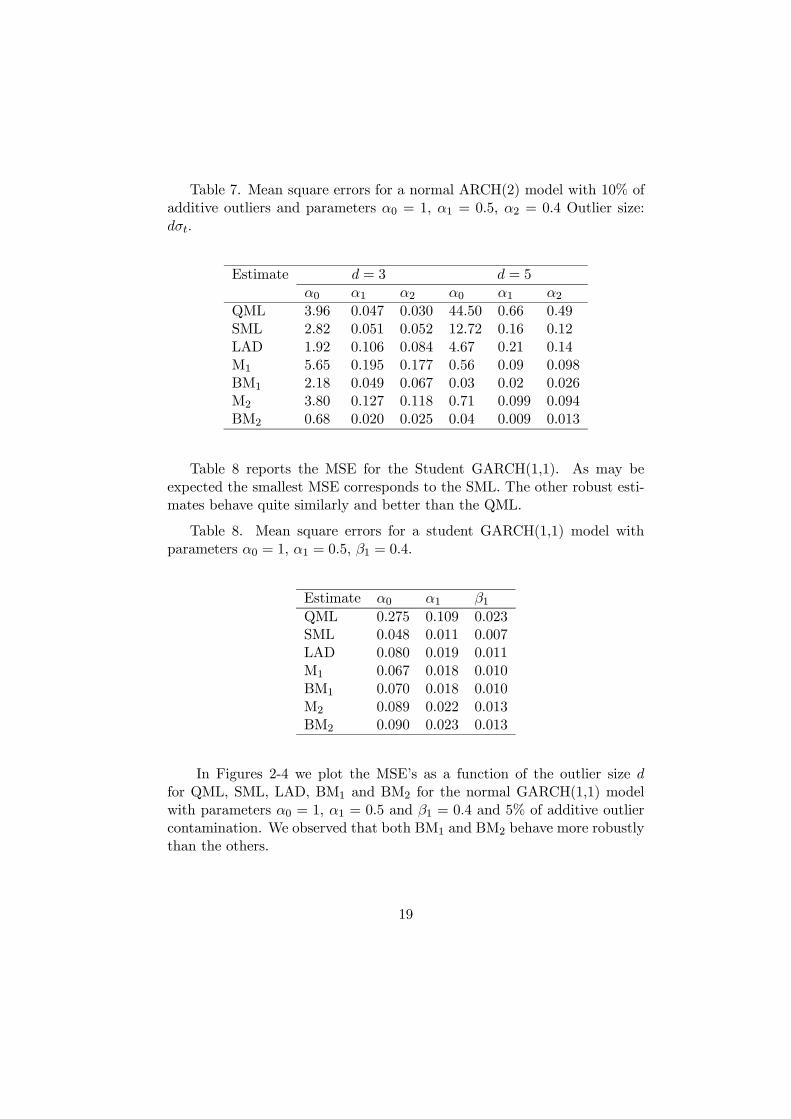
Table 8 reports the MSE for the Student GARCH(1,1). As may beexpected the smallest MSE corresponds to the SML. The other robust esti-mates behave quite similarly and better than the QML.
Table 8. Mean square errors for a student GARCH(1,1) model withparameters α0 = 1, α1 = 0.5, β1 = 0.4.
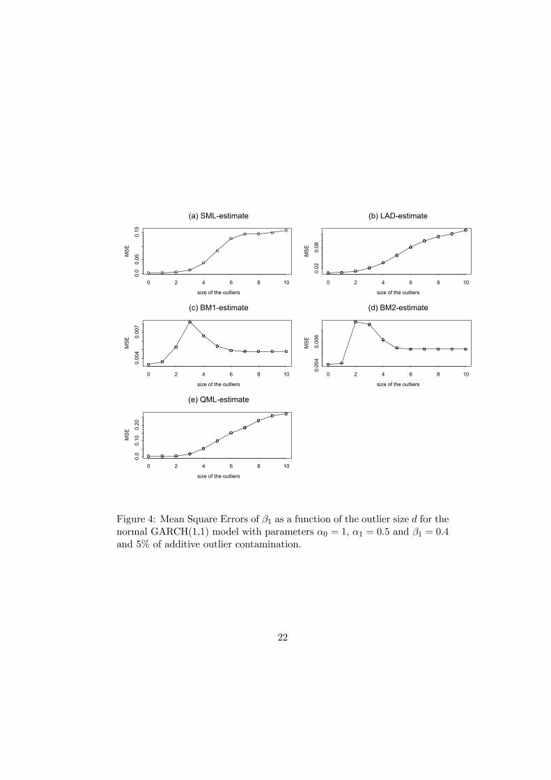
In Figures 2-4 we plot the MSE’s as a function of the outlier size dfor QML, SML, LAD, BM1 and BM2 for the normal GARCH(1,1) modelwith parameters α0 = 1, α1 = 0.5 and β1 = 0.4 and 5% of additive outliercontamination. We observed that both BM1 and BM2 behave more robustlythan the others.
19
size of the outliers
MSE
0 2 4 6 8 10
02
46
(a) SML-estimate
size of the outliers
MSE
0 2 4 6 8 10
0.5
1.5
(b) LAD-estimate
size of the outliers
MS
E
0 2 4 6 8 10
0.05
0.15
0.25
(c) BM1-estimate
size of the outliers
MS
E
0 2 4 6 8 10
0.10
0.20
(d) BM1-estimate
size of the outliers
MS
E
0 2 4 6 8 10
040
8012
0
(e) QML-estimate
Figure 2: Mean Square Errors of α0 as a function of the outlier size d for thenormal GARCH(1,1) model with parameters α0 = 1, α1 = 0.5 and β1 = 0.4and 5% of additive outlier contamination.
20
size of the outliers
MSE
0 2 4 6 8 10
0.0
0.10
0.20
(a) SML-estimate
size of the outliers
MSE
0 2 4 6 8 10
0.05
0.15
(b) LAD-estimate
size of the outliers
MS
E
0 2 4 6 8 10
0.00
40.
008
0.01
2
(c) BM1-estimate
size of the outliers
MS
E
0 2 4 6 8 10
0.00
60.
009
(d) BM2-estimate
size of the outliers
MS
E
0 2 4 6 8 10
0.0
0.4
0.8
1.2
(e) QML-estimate
Figure 3: Mean Square Errors of α1 as a function of the outlier size d for thenormal GARCH(1,1) model with parameters α0 = 1, α1 = 0.5 and β1 = 0.4and 5% of additive outlier contamination.
21
size of the outliers
MSE
0 2 4 6 8 10
0.0
0.05
0.15
(a) SML-estimate
size of the outliers
MSE
0 2 4 6 8 10
0.02
0.08
(b) LAD-estimate
size of the outliers
MSE
0 2 4 6 8 10
0.00
40.
007
(c) BM1-estimate
size of the outliers
MSE
0 2 4 6 8 10
0.00
40.
006
(d) BM2-estimate
size of the outliers
MS
E
0 2 4 6 8 10
0.0
0.10
0.20
(e) QML-estimate
Figure 4: Mean Square Errors of β1 as a function of the outlier size d for thenormal GARCH(1,1) model with parameters α0 = 1, α1 = 0.5 and β1 = 0.4and 5% of additive outlier contamination.
22
Observation Index
S&P
500
0 100 200 300 400 500 600
-0.0
40.
00.
04
Observation Index
SBS
E
0 100 200 300 400 500
-0.4
-0.2
0.0
0.2
0.4
Observation Index
EFC
X
0 100 200 300 400
-0.2
0.0
0.2
0.4
0.6
Observation Index
RH
O
0 100 200 300 400 500
-0.1
5-0
.05
0.05
Figure 5: Plot of the Daily Return Series.
5 Analysis of Some Examples
We consider four different examples of series corresponding to daily financialdata: (a) The Standard and Poor 500 Index (S&P 500) from February 1,2000 to June 30, 2002 (b) The SBS Technologies Inc.(SBSE) from January 3,2000 to December 31, 2001 (c) Electric Fuel. Corp (EFCX) from January 3,2000 to December 31, 2001 and (d) Rohm and Haas Company (ROH) fromJanuary 3, 2000 to December 31, 2001. In Fig 5 we plot the daily returnsof these four series. We observe that the series contain several outliers thatcorrespond to unusually large movements in the prices.
After centering with the median, each of these series was fitted as a
23
GARCH(1,1) model using the QML-estimate, SML-estimate, LAD-estimateand BM1-estimate defined as in the Section 4. In Table 9 we show theseestimates. Since the series contain outliers, as can be expected, the estimatesshow some important differences.
Table 9. Fitted GARCH(1,1) models for the daily returns series.
Let xt, 1 ≤ t ≤ T, be an observed centered series and (bα0, bα1, bβ1) anestimate for the GARCH(1,1) model. Let bσ2t be the conditional variance ofxt obtained using the estimated parameters. In the case of the QML-, SML-and LAD-estimates, bσ2t is recursively computed by
bσ2t = bα0 + bα1x2t−1 + bβ1bσ2t−1, 2 ≤ t ≤ T. (24)
In the case of the BM1- and the BM2-estimate bσ2t is also given by (24) if(bα0, bα1, bβ1) coincides with the correspondingM−estimate bγ1 defined in (14)or by
bσ2t = bα0 + bα1bσ2t−1gk(x2t−1/bσ2t−1) + bβ1bσ2t−1, 2 ≤ t ≤ Tif (bα0, bα1, bβ1) coincides with the bounded estimate bγ2 defined in (17).
When xt follows a GARCH model, the series zt have the following twoproperties (a) var(zt)=1 and (b) z
2t is uncorrelated to z
2t−1. We use these
properties to evaluate the performance in the four data sets of the differentestimates.
24
Given an estimate (bα0, bα1, bβ1) let us definebzt = xtbσt , 2 ≤ t ≤ T. (25)
If this estimate use to define bσt is close to the true value, properties (a)and (b) should approximately hold for the bz0ts.
Since the sample variance is not robust, to compare how property (a) issatisfied for the different estimates we use a normalized 0.10-trimmed samplevariance of bzt defined by
σ2TR =1.605
T1
T1Xt=1
bz2(t), (26)
where bz2(1) ≤ ... ≤ bz2(T−1) are the order statistics of ¡bz22 , ..., bz2T ¢, T1 is theinteger part of 0.9(T−1). The value 1.605 was chosen so that the normalizedtrimmed variance be one for normal samples. To compare the estimates inreference to property (b) we compute the rank correlation between bz2t−1 andbz2t , which is a robust correlation measure. We denote this estimate by τ.
Table 10 shows the value of σ2TR and τ corresponding to the QML-,SML-, LAD- and BM1-estimates for the four series.
Table 10. Truncated variance (σ2TR ) and rank correlation (τ) for thedaily returns series.
We observe that value of σ2TR for QML is in general much lower than one.Instead the robust estimates give values closer to one. In general all theestimates give values of τ close to zero. Taking into account both indicatorsσ2TR and τ, the BM-estimate performs better than the others for series S&P500, SBSE and RHO. However, for EFCX the SML seems preferable to theothers.
25
6 Concluding Remarks.
In this paper we present two classes of robust estimates for GARCH mod-els: M- and BM-estimates. A Monte Carlo study shows that for theGARCH(1,1) model, the QML-estimate may practically collapse when thereis 5% outlier contamination. All the robust estimates are in general lessinfluenced by outliers. However, the BM-estimates generally behave muchbetter than the rest of the robust methods under outlier contamination.
The study of four examples of daily returns series containing outliersshows that all the robust estimates are better than the QML-estimate. TheBM-estimate seems to behave better than the others in three of these ex-amples.
Our proposal is to always compute the BM- and the QML-estimateswhen fitting a GARCH model. A strong discrepancy between the two esti-mates indicates the presence of outliers in the series. In this case the decisionof which estimate is preferable can be based on the comparison of the sta-tistics σ2TR and τ for both fits. Of course this strategy can include otherrobust estimates such as the LAD or the SML.
7 Appendix
Proof of Lemma 1.We have that
E(|wt|) =Z ∞−∞
¯log(z2)
¯f(z)dz. (27)
Since f is continuous, there is a constant K such that |f(z)| ≤ K for allz ∈ [−1, 1]. Then we haveZ
|z|≤1
¯log(z2)
¯f(z)dz ≤ K
Z|z|≤1
¯log(z2)
¯dz <∞. (28)
Since for u ≥ 1 it holds that log(u) < u. Then using that zt has finitesecond moment we getZ
|z|>1
¯log(z2)
¯f(z)dz ≤
Z|z|>1
z2f(z)dz <∞. (29)
Then part (a) of the Lemma follows from (27),(28) and (29).Then (b) follows from (a) and the fact that ρ satisfies a global Lipschitz
condition.
26
Proof of Theorem 1.(i) Let γ = (α,β) be the true parameter. Then, we can write
M(c) = E
Ãρ
Ãwt − log
Ãeht(c)eht(γ)!!!
, (30)
where wt = log(yt/eht(γ)) = log(z2t ) are i.i.d. random variables with distri-bution g. Since eht(c) depends only on xt∗ with t∗ < t and E(ρ (wt − u))has a unique minimum at u0, the minimum of M(c) is attained at a pointc such that eht(c) = eu0eht(γ) a.s..Let γ∗ = (eu0α0, eu0α1, ..., eu0αp,β1, ...,βq), then we have eht(γ∗) = eu0eht(γ)and so eht(c) = eht(γ∗). Therefore, from Corollary 2.1 of Berkes, Horvathand Kokoszka (2003), we obtain c = γ∗.
(ii) Since g is strictly unimodal, continuous and g(u) > 0 for all u, Lemma1 of Bianco, Garcia Ben and Yohai (2005) implies that E(ρ (wt − u)) has aunique minimum at u0 = 0. Hence, (ii) follows
According to the Remark after Theorem 1, in the rest of the Appendixwe will assume u0 = 0 and γ
∗ = γ without loss of generality.The following Lemmas 2, 3 and 4 are used in the proofs of Theorems 2
and 3.Lemma 2. Let xt be a stationary and ergodic GARCH(p, q) process sat-
isfying (1) and(2). Let ht(c) be as defined in (8) and eht(c) as defined in(20). Then
(i) There exists 0 < ϑ < 1 and a positive finite random variable W such
that supc∈C
¯eht(c)−ht(c)¯ ≤ ϑtW for all t ≥ p+ 1.(ii)There exists a neighborhood U of γ such that sup
c∈UE¯∇ log(eht(c))¯n <
∞ for all n.(iii)There exists a neighborhood U of γ, 0 < ϑ < 1 and a finite positive
finite random variable W1 such that
supc∈U
¯∇ log(eht(c))−∇ log(ht(c))¯ ≤ ϑtW1
for all t ≥ p+ 1.(iv)There exists a neighborhood U of γ, 0 < ϑ < 1 and a positive finite
Observe that sup(a,b)∈CPqi=1 bi < 1 implies thatW <∞ and since 0 < eb <
1 we also have 0 < ϑ < 1.(ii) is proved in Hall and Yao (2003).(iii) Hall and Yao (2003) derive the following formulas
∂eht(c)∂a0
=1
1−Pqj=1 bj
, (33)
∂eht(c)∂ai
= x2t−i +∞Xk=1
qXji=1
· · ·qX
jk=1
bj1 · · · bjkx2t−i−j1−···−jk , 1 ≤ i ≤ p, (34)
∂eht(c)∂bj
=a0
(1−Pqi=1 bi)
2
+pXi=1
ai
∞Xk=0
(k + 1)qX
ji=1
· · ·qX
jk=1
bj1 · · · bjkx2t−i−j1−···−jk , 1 ≤ j ≤ q.(35)
In a similar way, from (32) we can derive
∂ht(c)
∂a0=
1
1−Pqj=1 bj
, (36)
∂ht(c)
∂ai= x2t−i +
∞Xk=1
qXji=1
· · ·qX
jk=1
bj1 · · · bjkx2t−i−j1−···−jkIt−i−j1−···jk≥1 (37)
and
29
∂ht(c)
∂bj=
a0
(1−Pqi=1 bi)
2 + (38)
+pXi=1
ai
∞Xk=0
(k + 1)qX
ji=1
· · ·qX
jk=1
bj1 · · · bjkx2t−i−j1−···−jkIt−i−j1−···jk≥1
for t ≥ p+ 1 and c = (a,b). Then we get
∂eht(c)∂a0
− ∂ht(c)
∂a0= 0, (39)
0 ≤ ∂eht(c)∂ai
− ∂ht(c)
∂ai≤
∞Xk=kt
qXji=1
· · ·qX
jk=1
bj1 · · · bjkx2t−i−j1−···−jk (40)
and
0 ≤ ∂eht(c)∂bj
− ∂ht(c)
∂bj≤
pXi=1
ai
∞Xk=kt
(k + 1)qX
ji=1
· · ·qX
jk=1
bj1 · · · bjkx2t−i−j1−···−jk ,
(41)where kt is the integer part of (t − p − 1)/q. Consider a neighborhood Uof γ such U ⊂ Cδ0/2, then, using a similar argument than the one used theproof of (i), we can prove that there exists ϑ1, 0 < ϑ1 < 1, and a randomvariable W ∗
1 such that
supc∈U
¯¯∂eht(c)∂ai
− ∂ht(c)
∂ai
¯¯ ≤ ϑt1W
∗1 . (42)
A similar bound can be obtained for the right hand side of (41) as follows
pXi=1
ai
∞Xk=kt
(k + 1)qX
ji=1
· · ·qX
jk=1
bj1 · · · bjkx2t−i−j1−···−jk
≤ ebkt−1 pXi=1
ai
∞Xk=1
(kt + k)qX
ji=1
· · ·qX
jk=1
bj1 · · · bjkx2t−i−j1−···−jk ,
where eb = maxC {max(b1, ..., bq), (a,b) ∈C} .30
There exists 0 < b∗ < 1 and t0 such that for t ≥ t0 we haveebkt−1kt ≤ ebt/qteb−p/q−2 ≤ (b∗)t eb−p/q−2.
and from Hall and Yao (2003) we know that the random variables
supc∈U
pXi=1
ai
∞Xk=1
qXji=1
· · ·qX
jk=1
bj1 · · · bjkx2t−i−j−j1−···−jk
and
supc∈U
pXi=1
ai
∞Xk=1
kqX
ji=1
· · ·qX
jk=1
bj1 · · · bjkx2t−i−j−j1−···−jk
are finite. Then taking ϑ2 = b∗ and
W ∗2 =
eb−p/q−2 sup(a,b)∈C
pXi=1
ai
∞Xk=1
(1 + k)qX
ji=1
· · ·qX
jk=1
bj1 · · · bjkx2t−i−j1−···−jk
we obtain
supc∈U
¯¯∂eht(c)∂bj
− ∂ht(c)
∂bj
¯¯ ≤ ϑt2W
∗2 (43)
for t ≥ t0 where W ∗2 is a finite random variable.
From (39),(42) and (43) we get that there exists a constant 0 < ϑ3 < 1and a finite random variable W ∗
3 such that
supc∈U
¯∇eht(c)−∇ht(c)¯ ≤ ϑt3W
∗3 (44)
for t ≥ t0Since c ∈U ⊂ Cδ0/2, from (21) we obtain
eht(c) ≥δ0/2, ht(c) ≥δ0/2. (45)
We can write
∇ log eht(c)−∇ log ht(c)=
1
ht(c)eht(c)∇eht(c)³ht(c)− eht(c)´+ 1
ht(c)(∇eht(c)−∇ht(c)),
31
and so from (i), (ii), (44) and (45) we prove (iii).(iv) We can write
∇ log(eht(c))∇ log(eht(c))0−∇ log(ht(c))∇ log(ht(c))0= ∇ log(eht(c))(∇ log(eht(c))−∇ log(ht(c)))0+³∇ log(eht(c))−∇ log(ht(c))´∇ log(ht(c))0Then using (ii) and (iii) we get (iv).(v) This is shown by Peng and Yao (2003) while proving Theorem 1.(vi) The proof is similar to that of (iv) using the expression for ∇2eht(c)
given in Peng and Yao (2003).Lemma 3. Let C be as in (21) and
fMT (c) =1
T − pTX
t=p+1
ρ(yt − log eht(c)). (46)
Then under the assumptions of Theorem 2, have
limT→∞
supc∈C
¯ fMT (c)−M(c)¯= 0 a.s..
Proof.Proof.We start proving
E
Ãsupc∈C
(|ρ(yt − log eht(c))|)!<∞. (47)
Since ρ has a bounded derivative, it is enough to show that
E
Ãsupc∈C
(|yt − log eht(c)|)!<∞. (48)
We also have
yt − log eht(c) = wt + log eht(γ)− log(eht(c)).Since by Lemma 1 (a) E(|wt|) <∞, to prove (47) it is enough to show
that
E
Ãsupc∈C
(| log eht(c)|)!<∞. (49)
32
From (21) and (31) we have that
E(supc∈C
eht(c)) <∞, (50)
and from (21) we obtainδ0 ≤ inf
c∈Ceht(c). (51)
Then (49) follows from (50) and (51) and the Lemma follows from Lemma3 of Muler and Yohai (2002).Lemma 4.Under the assumptions of Theorem 2, we have
limT→∞
supc∈C
¯MT (c)− fMT (c)
¯= 0
a.s.Proof
We have
MT (c)−fMT (c) =1
(T − p)TX
t=p+1
³ρ³yt − log
³eht(c)´´− ρ (yt − log (ht(c)))´.
Let K = sup |ρ0| < ∞. Then, from Lemma 2-(i) and (21) we have thatthere exists 0 < ϑ < 1, and a finite positive random variable W such that¯ρ³yt − log
³eht(c)´´− ρ (yt − log (ht(c)))¯≤ K
δ0
¯eht(c)− ht(c)¯ ≤ Kδ0ϑtW,
and this proves the Lemma.Proof of Theorem 2.
From Lemmas 3 and 4 we get
limT→∞
supc∈C
|MT (c)−M(c)| = 0
a.s. Then, putting
A =
(supc∈C
|MT (c)−M(c)|→ 0
),
we have P (A) = 1. Therefore it is enough to prove
A ⊂ { bγT → γ} . (52)
33
Assume that (52) is not true. Then we can find in A a subsequencebγTi such thatbγTi → γ (53)
with γ 6= γ. Since M(c) has a unique minimum at γ, and M(c) is continu-ous, there exists a neighborhood U(γ) and ε > 0 such that for all c ∈ U(γ)we obtain
M(c) > M(γ) + ε. (54)
From (53) there exists i0 large enough such that for all i ≥ i0 we obtain
bγTi ∈ U(γ), supc∈C
|MTi(c)−M(c)| <ε
2. (55)
Therefore from (54) and (55) for all i ≥ i0 we obtain
MTi(bγTi) =MTi(bγTi)−M(bγTi) +M(bγTi) > M(γ) + ε
2. (56)
Using the definition of bγT and (55), we haveMTi(bγTi) ≤MTi(γ) < M(γ) +
ε
2,
for all i ≥ i0. This contradicts (56) and therefore the Theorem is proved.We need the following four Lemmas to prove Theorem 3.
Lemma 5. Suppose that all the assumptions of Theorem 2 hold. More-over, assume that ρ has a continuous and bounded derivative ψ such thatE(ψ2(wt)) > 0. Then,
1√T − p
TXt=p+1
∇ρ³yt − log
³eht(γ)´´ →D N(0, E(ψ2 (wt))D0),
whereD0 = E
³∇ log(eht(γ))∇ log(eht(γ))0´ .
Proof.From Lemma 2-(ii) D0 is finite, and from (4) it can be shown that D0 is
positive definite (see for instance Horvath and Kokoszka (2003)).On the other hand, since E(ρ (wt − u)) is minimized at u = 0, we have
34
E(ψ(wt)) = 0.
This implies that b0ψ(wt )∇ log(eht(γ)) is a stationary martingale differencesequence for any vector b 6= 0 in Rp+q+1. Then applying the Central LimitTheorem for Martingales (see for instance Theorem 24.4, Davidson(1994))we obtain
1√T − p
TXt=p+1
b0ψ(wt)∇ log(eht(γ)) →D N(0, E(ψ2 (wt))b
0 D0b).
Finally, using a standard Cramer-Wold device we get the desired result.Lemma 6. Suppose that all the assumptions of Lemma 5 hold. More-over, assume that ρ has a two continuous and bounded derivatives and thatE(ψ0(wt)) > 0. Define A(c) = E(∇2ρ(yt − log(eht(c)))), then there exists aneighborhood U of γ such that
(i)
limT→∞
supc∈U
°°°°°° 1
T − pTX
t=p+1
∇2ρ(yt − log(eht(c)))−A(c)°°°°°° = 0 a.s..
(ii) A(γ) is a positive definite matrix given by A(γ) = E(ψ0(wt))D0.
From (21) and Lemma 2-(v) there exists a neighborhood U of γ suchthat
E
Ãsupc∈U
°°°°°∇2eht(c)eht(c)°°°°°!<∞. (58)
35
Then by Lemma 2-(ii), (57), (58) and the fact that ψ and ψ0 are continuousand bounded we get
E supc∈U
°°°∇2ρ ³yt − log ³eht(c)´´°°° <∞.Therefore, part (i) of the Lemma follows from Lemma 3 of Muler and Yohai(2002).
Since E(ψ(wt)) = 0 and yt − log(eht(γ)) = wt we getE(ψ(yt − log(eht(γ))∇ log(eht(γ))∇ logf(ht(γ))) = 0
and
E
Ãψ(yt − log(eht(γ)))∇2eht(γ)eht(γ)
!= 0.
ThenA(γ) = E(ψ0(wt))D0.
Since D0 is positive definite and E(ψ0(wt)) > 0 part (ii) follows.
Lemmas 7 and 8 are necessary to show that the asymptotic distributionof the M-estimates can be derived using the eht(γ)’s instead of the ht(γ)’s.Lemma 7. Suppose that all the assumptions of Lemma 6 hold. Then
³eht(c)´∇ log ³eht(c)´0 .From Lemma 2-(iv) there exists a neighborhood U1 of γ with U1 ⊂
Cδ0/2, 0 < ϑ < 1 and a finite random variable W2 such that
supc∈U1
kQt(c)k < ϑtW2
for t ≥ p+ 1. Then
limT→∞
supc∈U1
1
T − pTX
t=p+1
kQt(c)k = 0 (68)
a.s.. Then, since ζ(yt − log(ht(c))) is bounded we obtain
limT→∞
supc∈U1
1
T − pTX
t=p+1
kζ(yt − log(ht(c)))Qt(c)k = 0 (69)
a.s.. From Lemma 2-(ii) we have that there exists a neighborhood U2 ⊂ U1of γ such that,
E
Ãsupc∈U2
°°°°∇ log ³eht(c)´∇ log ³eht(c)´0°°°°!<∞. (70)
Since ζ 0 is bounded and U2 ⊂ Cδ0/ 2 , applying Lemma 2-(i) and usingsimilar arguments that in the proof of Lemma 7, we obtain
limT→∞
supc∈U2
1
T − pTX
t=p+1
³ζ(yt − log(eht(c)))− ζ(yt − log(ht(c)))
´∇ log
³eht(c)´∇ log ³eht(c)´0 = 0(71)
a.s.. Then, by (67), (69) and (71) we have
limT→∞
supc∈U2
1
T − pTX
t=p+1
Ht(c) = 0 (72)
a.s..
39
From Lemma 2-(vi) and Lemma 2-(v) there exists a neighborhood U ⊂U2 of γ, a constant 0 < ϑ < 1 and a positive variable W3 such that for allt ≥ p+ 1
supc∈U
°°°°°∇2eht(c)eht(c) − ∇2ht(c)
ht(c)
°°°°° ≤ ϑtW3,
and
supc∈U
E
°°°°°∇2eht(c)eht(c)°°°°°2
<∞.
Then, since ψ0 is bounded and U ⊂ Cδ0/2 using similar arguments than inthe proof of Lemma 7, we can show
limT→∞
supc∈U
1
T − pTX
t=p+1
Gt(c) = 0 (73)
a.s.. Finally, the Lemma follows from (72) and (73).Proof of Theorem 3
From Lemmas 5 and 7 we have
1√T − p
TXt=p+1
∇ρ (yt − log (ht(γ))) →D N(0, E(ψ2 (wt))D0), (74)
and from Lemmas 6-(i) and 8 we get that there exists a neighborhood U ofγ such that
limT→∞
supc∈U
°°°°°° 1
T − pTX
t=p+1
∇2ρ (yt − log (ht(c)))−A(c)°°°°°° = 0 a.s.. (75)
From (74) and (75) and Theorem 2 we get that
1
T − pTX
t=p+1
∇2ρ (yt − log (ht(c)))
is continuous in c, and that A0 = A(γ) is nonsingular (Lemma 6-(ii)). Then,Theorem 3 follows from Theorem 4.1.3. of Amemiya (1985).
40
The following Lemmas 9, 10 and 11 are going to be used to prove The-orem 4.Lemma 9. Let Yt be an ergodic process in R
m and g : Rm × R → R, acontinuous function satisfying:
(i) There exists g0 : Rm → R such that |g(Yt, u)| ≤ g0(Yt), and g0(Yt)
integrable.
(ii) limu→∞ g(Yt, u) = g+(Yt) and limu→−∞ g(Yt, u) = g−(Yt). Then
limT→∞
supu∈ R
¯¯ 1T
TXt=1
g(Yt, u)−E (g(Yt, u))¯¯ = 0 a.s..
Proof.From Muler and Yohai (2002) we have
limT→∞
supu∈ K
¯¯ 1T
TXt=1
g(Yt, u)−E (g(Yt, u))¯¯ = 0 a.s. (76)
for any compact set K ⊂R. Then to prove the Lemma, it is enough to showthat given any ε, there exists u such that
limT→∞
supu≥u
¯¯ 1T
TXt=1
g(Yt, u)−E (g(Yt, u))¯¯ ≤ ε a.s. (77)
and
limT→∞
supu≤u
¯¯ 1T
TXt=1
g(Yt, u)−E (g(Yt, u))¯¯ ≤ ε a.s..
Since both proofs are similar we only show (77). To this purpose, it isenough to prove that
limT→∞
supu≥u
1
T
TXt=1
g(Yt, u)−E (g(Yt, u)) ≤ ε a.s. (78)
and
limT→∞
infu≥u
1
T
TXt=1
g(Yt, u)−E (g(Yt, u)) ≥ −ε a.s.. (79)
41
Since the proofs of (78) and (79)are similar, we only show (78).Let
Bt(v) = supu>v(g(Yt, u)−E(g(Yt, u)).
Clearly, by the Dominated Convergence Theorem we have limv→∞Bt(v) =g+(Yt) − E(g+(Yt)) and limv→∞ E(Bt(v)) = 0. Therefore there exists usuch that E(Bt(u)) < ε. Then using the Law of Large Numbers we get
limT→∞
supu≥u
1
T
TXt=1
g(Yt, u)−E (g(Yt, u)) ≤ limT→∞
1
T
TXt=1
Bt(u) ≤ ε a.s.
and this proves (78).Lemma 10. Suppose that all the assumptions of Theorem 2 hold. Then,we have that
supc∈C
h∗t,k(c) ≤ Rt,
where h∗t,k(c) is defined in (15) and Rt is a positive-valued ergodic process.Proof.
Define
Rt = supc∈C
eht(c). (80)
Then, from (21) and (31) we have that Rt is a positive-valued ergodicprocesses and from (8) we get
supc∈C
ht(c) ≤ Rt. (81)
We prove by induction on t that
h∗t,k(c) ≤ ht(c). (82)
From the (15) it follows immediately that
h∗t,k(c) = ht(c) (83)
for all t ≤ 0. Assume now
h∗j,k(c) ≤ hj(c), j ≤ t.Then from (15) we have
42
h∗t+1,k(c) ≤ a0 +pXi=1
aix2t+1−i +
qXi=1
bih∗t+1−i,k(c) ≤ ht+1(c), (84)
and thereby (82) follows. Then, the Lemma follows from (81).Lemma 11. Suppose that all the assumptions of Theorem 4 hold. Letm0 = E(ρ(wt)) = J(0). Then, there exists δ > 0 such that
lim infT→∞
infc∈C
M∗Tk(c) > m0 + δ a.s.,
where M∗Tk is given in (18).
Proof.Since γ ∈C, there exists i0, 1 ≤ i0 ≤ p such that αi0 > 0. Then
eht(γ) ≥ αi0x2t−i0 = αi0z
2t−i0
eht−i0(γ). (85)
Consider s = max(p, q). If p < s define ap+1 = · · · = as = 0 and αp+1 =· · · = αs = 0. If q < s define bq+1 = · · · = bs = 0 and βq+1 = · · · = βs = 0.Then, we have for all t ≥ 1
h∗t,k(c) ≤ a0 +sXi=1
(aik + bi)h∗t−i,k(c) ≤ (2 + k)
sXi=1
h∗t−i,k(c) (86)
and
sXi=1
h∗t−i,k(c) ≤ (2+k)sXi=1
h∗t−i−1,k(c)+sXi=2
h∗t−i,k(c) ≤ 2(2+k)sXi=1
h∗t−i−1,k(c).
(87)By Lemma 10, there exists a positive-valued ergodic process Rt such
that supc∈C h∗t,k(c) ≤ Rt. Then, from (86) and (87) we have that
h∗t,k(c) ≤ 2i0(2 + k)i0+1s+jXi=j+1
Rt−i. (88)
Let us define the ergodic processes
Nt =eht−i0(γ)s+i0Pi=i0+1
Rt−i, t ≥ 1.
Then there exists η > 0 and ν > 0 such that
43
P (Nt > η ) ≥ ν. (89)
Using that limu→∞ ρ(u) = supu ρ(u) > m0, it is easy to show that if ε issmall enough, there exists k1 > 0 such that
infu≤−k1
E(ρ(wt − u)) ≥ m0 + ε. (90)
Let us define K as
K =2i0(2 + k)i0+1ek1
ηαi0(91)
and define
At =nNt > η, z2t−i0 > K
o. (92)
Since z2t−i0 is independent ofNt, using (89) and the fact that zt is unbounded,we have
a = P (At) = νP (z2t−i0 > K) > 0. (93)
From (88), (85) and the choice of K in the definition of At we have
supc∈C
(log h∗t,k(c)− log eht(γ)) ≤ −k1. (94)
We can write
M∗Tk(c) =
1
T − pTX
t=p+1
ρ(wt + log(eht(γ))− log(h∗t,k(c))).Let us consider first the case when ρ is a bounded function. From (94) weobtain
infc∈C
M∗Tk(c) ≥ inf
u
1
T − pTX
t=p+1
ρ(wt − u)(1− IAt)
+ infu≤−k1
1
T − pTX
t=p+1
ρ(wt − u)IAt . (95)
Since ρ is bounded, lim|u|→∞ ρ(u) = supu ρ(u) and IAt is ergodic and inde-pendent of wt, from Lemma 9 we get
44
limT→∞
supu
¯¯ 1
T − pTX
t=p+1
ρ(wt − u)(1− IAt)−E (ρ(wt − u)) (1− a)¯¯ = 0 a.s.
(96)and
limT→∞
supu≤−k1
¯¯ 1
T − pTX
t=p+1
ρ(wt − u)IAt −E (ρ(wt − u)) a¯¯ = 0 a.s.. (97)
From (96) and using E (ρ(wt − u)) ≥ m0 > 0 we get
lim infT→∞
infu
1
T − pTX
t=p+1
ρ(wt − u)(1− IAt ) ≥ m0(1− a) a.s.,
and from (90) and (97) we obtain
lim infT→∞
infu≤−k1
1
T − pTX
t=p+1
ρ(wt − u)IAt ≥ (m0 + ε)a a.s..
Thus, from (95) we derive
lim infT→∞
infc∈C
M∗Tk(c) ≥ m0 + εa a.s.,
and then taking δ = εa, the Lemma follows for the case that ρ is bounded.Consider now the case that lim|x|→∞ ρ(x) = ∞. We start proving that
for any k ≥ 0,E( sup
|u|≤kρ(wt − u)) <∞. (98)
Take any sequence ui with |ui | ≤ k, then
lim supi→+∞
E(ρ(wt − ui)) = lim supi→+∞
E (ρ(wt − ui)− ρ(wt)) +E(ρ(wt))
≤ k supu
ρ0(u) +E(ρ(wt)),
and (98) is proved.We will prove that there exists k1 large enough such that
45
lim infT→∞
supu≤−k1
1
T − pTX
t=p+1
ρ(wt − u)IAt ≥ 2m0a a.s. (99)
Given D > 0, define BtD = {|wt| ≤ D} and let D0 be such P (BtD0) ≥ 1/2.Let d1 be such that for all |x| ≥ d1 we have ρ(x) ≥ 4m0 and put k1 =2D0 + d1. Then,
lim infT→∞
supu≤−k1
1
T − pTX
t=p+1
ρ(wt − u)IAt
≥ lim infT→∞
supu≤−k1
1
T − pTX
t=p+1
ρ(wt − u)IAtIBtD0
≥ 4m0 lim infT→∞
1
T − pTX
t=p+1
IAtIBtD0 = 4m0E(IAtIBtD0 ).
Since At and Bt are independent, P (BtD0) ≥ 1/2 we obtain (99).We prove now
lim infT→∞
infu
1
T − pTX
t=p+1
ρ(wt − u)(1− IAt) ≥ m0 (1− a) a.s.. (100)
To prove this it is enough to show that
limD→∞
lim infT→∞
infu
1
T − pTX
t=p+1
ρ(wt − u)(1− IAt)IBtD ≥ m0 (1− a) a.s..(101)
Since lim|x|→∞ ρ(x) =∞, there exists a compact set UD ⊂ R such that
infu
1
T − pTX
t=p+1
ρ(wt−u)(1−IAt)IBtD = infu∈UD
1
T − pTX
t=p+1
ρ(wt−u)(1−IAt)IBtD ,
and so using compacity arguments and the fact that IAt is independent ofwt and of BtD we have that
lim infT→∞
infu∈UD
1
T − pTX
t=p+1
ρ(wt − u)(1− IAt)IBtD
46
≥ infu∈UD
E (ρ(wt − u)IBtD) (1− a)≥ inf
uE (ρ(wt − u)IBtD) (1− a).
Then to prove (100) it is enough to show that
limD→∞
infuE (ρ(wt − u)IBtD) = m0. (102)
Suppose that (102) is not true. Then, there exists (un,Dn) such thatDn ↑ ∞and ε > 0 such that
E³ρ(wt − un)IBtDn
´< m0 − ε. (103)
Without loss of generality, taking if necessary a subsequence, we have toconsider only the following two cases
(i) limn→∞un = u.
(ii) limn→∞ |un| =∞.
We have that
limn→∞ ρ(wt − un)IBtDn = ρ(wt − u)
Sincesup
|u|≤2|u|ρ(wt − u)
has finite expectation, by the dominated convergence theorem we get
lim infn→∞ E
³ρ(wt − un)IBtDn
´= E(ρ(wt − u)) ≥ m0
contradicting (103). This proves (102) for the case (i).Consider now case (ii). LetD0, d1 and k1 as in the proof of (99). Observe
that in BtD0 the condition |u| ≥ k1 implies |wt − u| ≥ d1 and therefore
limn→∞E
³ρ(wt − un)IBtDn
´≥ inf|u|≥k1
E³ρ(wt − u)IBtD0
´≥ 4m0P (BtD0) ≥ 2m0
contradicting (103). This proves (102) for the case (ii). This completes theproof of the Lemma for the case of unbounded ρ.Proof of Theorem 4.
Let bγ2 be as defined in (17). From Lemma 11 we have that
lim infT→∞
M∗Tk(bγT,2) > m0 + δ a.s.
47
for some δ > 0. On the other hand, by Theorem 2 we have that bγT as definedin (14) satisfy limT→∞MT (bγT ) = m0. This proves the Theorem.
Acknowledgments. This research was partially supported by a grantfrom the Fundacion Antorchas, Argentina, grant X611 from the University ofBuenos Aires and grant 03—06277 from the Agencia Nacional de PromocionCientifica y Tecnologica, Argentina.
REFERENCES
Amemiya, T. ,1985, Advanced Econometrics. Cambridge, Harvard Univer-sity Press.
Berkes, I., Horvath, L. and P. Kokoszka , 2003, GARCH processes: struc-ture and estimation. Bernoulli 9, 201-207.
Bianco, A. M., Garcia Ben, M. and V. J. Yohai , 2005, Robust estima-tion for linear regression with asymmetric errors, Canadian Journal ofStatistics, 33.
Bianco, A. M., Garcia Ben, M., Martinez, E. J. and V.J. Yohai , 1996, Ro-bust procedures for regression models with ARIMA Errors’, COMP-STAT 96, Proceedings in Computational Statistics, 27—38, Physica-Verlag.
Boente, G. , Fraiman, R. and V. J. Yohai, 1987, Qualitative robustness forgeneral stochastic processes, Annals of Statistics, 15, 1293-1312.
Bollerslev, T. , 1986, Generalized autoregressive conditional heteroskedas-ticity, Journal of Econometrics, 31, 307-27.
Bollerslev, T. , Chou, R. and K. Kroner,1992, ARCH modelling in finance:a review of theory and empirical evidence, Journal of Econometrics,52, 5-60.
Bougerol, P. and N. Picard, 1992, Stationarity of GARCH processes and ofsome nonnegative time series, Journal of Econometrics, 52, 115-127.
Boussama, F, 2000, Asymptotic normality for the quasi-maximum likeli-hood estimator of a GARCH model, Comptes Rendus de l’Academiedes Sciences Paris, Serie I, 331, 81-84.
48
Carnero, A., Pena, D. and E. Ruiz, 2001, Outliers and conditional autore-gressive heteroscedasticity in time series, Estadistica, 53, 143-213.
Davidson, J. , 1994, Stochastic Limit Theory: An Introduction for Econo-metricians, New York: Oxford University Press.
Denby, L. and R. D. Martin, 1979, Robust estimation of the first—orderautoregressive parameter, Journal of the American Statistical Associ-ation, 74, 140—146.
Elie, L. and T. Jeantheau, 1995, Estimation in conditionally heteroskedas-tic models, Comptes Rendus de l’Academie des Sciences Paris, SerieI, 320, 1255-1258.
Engle, R. F., 1982, Autoregressive conditional heteroscedasticity with es-timates of the variance of UK inflation, Econometrica, 50, 987-1008.
Engle, R. F., Lilien, D. M. and R. P. Robins, 1987, Estimating time-varyingrisk premia in the term structure: the ARCH-Mmodel, Econometrica,55, 391-407.
Christian F. and J. M.. Zakoian, 2004, Maximum likelihood estimation ofpure GARCH and
ARMA-GARCH processes, Bernoulli 10, 605-637.
Franses, P. H. and D. van Dijk, 2000, Outlier detection in GARCH models.Research report EI-9926/RV, Econometric Institute, Erasmus Univer-sity, Rotterdam.
Geweke, J. , 1986, Comment- modeling persistency of conditional variances,Econometric Review, 5, 57-61.
Giraitis, L., Kokoszka, P. and R. Leipus, 2000, Stationary ARCH mod-els: dependence structure and Central Limit Theorem, EconometricTheory, 16, 3-22.
Hampel, F., 1971, A general qualitative definition of robustness, Annals ofMathematical Statistics, 42, 1887-1896.
Hall, P. and Q. Yao, 2003, Inference in ARCH and GARCH models withheavy-tailed errors, Econometrica, 71, 285-317.
49
Huber, P. J. , 1964, Robust estimation of a location parameter, Annals ofMathematical Statistics, 35, 73-101.
Huber, P. J., 1973, Robust regression: asymptotics, conjectures and MonteCarlo, Annals of Statistics, 1, 799-821.
Huber, P. J., 1981, Robust Statistics, Wiley, N. Y.
Jiang, J., Zhao, Q., and Y.V. Hui, 2001, Robust modelling of ARCH mod-els, Journal of Forecasting, 20, 111-133.
Lee, S. and B. Hansen, 1994, Asymptotic theory for the GARCH(1,1)Quasi-Maximum Likelihood estimator, Econometric Theory, 10, 29-52.
Li, J. and C. Kao, 2002, Bounded influence estimation and outlier de-tection for GARCH models with and application to foreign exchangerates, Working Paper presented at the 57th European Meeting of theEconometric Society.
Lumsdaine, R.L., 1996, Consistency and asymptotic normality of the Quasi-Maximum Likelihood Estimator in IGARCH(1,1) and covariance sta-tionary GARCH(1,1) models, Econometrica, 64, 575-596.
Martin, R. D., Samarov, A. and W. Vandaele, 1983, Robust methods forARIMA models, United States Bureau of Census, Applied Time SeriesAnalysis of Economic Data, 153—177.
Mendes, B.V. M. , 2000, Assessing the bias of maximum likelihood esti-mates of contaminated GARCH Models, Journal of Statistical Com-putation and Simulation., 67, 359-376.
Mendes, B.V. M. and A. M. Duarte, 1999, Robust estimation for ARCHmodels. Revista de Econometria, 19, 138-180.
Muler, N. and V. J. Yohai , 2002, Robust estimates for ARCH Processes,Time Series Analysis, 23 , 341-375.
Nelson, D. , 1990, Stationarity and persistence in the GARCH(1,1), Model.Econometric Theory, 6, 318-334.
Nelson, D. B., 1991, Conditional heteroskedasticity in asset returns: A NewApproach, Econometrica, 59, 347-370.
50
Park, B., 2002, An outlier robust GARCH model and forecasting volatilityof exchange rate returns, Journal of Forecasting, 21, 381-393.
Peng, L. and Q. Yao, 2003, Miscellanea. Least absolute deviations estima-tion for ARCH and GARCH models, Biometrika, 90, 967-975.
Rieder, H. , Ruckdeschel, P. and M. Kohl, 2002, Robust estimation for timeseries models based on infinitesimal neighborhoods, Working Paperpresented at ICORS 2002, Vancouver.
Ronchetti E. and F. Trojani, 2001, Robust inference with GMM estimators,Journal of Econometrics, 101, 37-69.
Sakata, S. and H. White,1998, High breakdown point conditional disper-sion estimation with application to S&P 500 daily returns volatility,Econometrica, 66 (3),529-567.
Straumann, D. and T. Mikosh, 2003, Quasi-maximum-likelihood estima-tion in heteroscedastic time series: a stochastic recurrence equationapproach. Technical report, University of Copenhagen.
van Dijk, D., Lucas, A. and P. H. Franses, 1999 Testing for ARCH in thepresence of additive outliers. Journal of Applied Econometrics, 14,539-562
Yohai, V.J., 1987, High breakdown-point and high efficiency robust esti-mates for regression, Annals of Statistics, 15, 642-656.