50
Robust estimation in time series V. A. Reisen NuMes, D.E; Universidade Federal do Espirito Santo, Brazil. 20 de setembro de 2011
| Date post: | 08-Mar-2018 |
| Category: |
Documents |
| Upload: | duongthien |
| View: | 215 times |
| Download: | 0 times |

Robust estimation in time series
V. A. Reisen
NuMes, D.E; Universidade Federal do Espirito Santo, Brazil.
20 de setembro de 2011

Contents
Abstract
Introduction-Co-authors references
Introduction-Examples
Introduction-some references
The impact of outliers in stationary processes
A robust estimator of ACF
Theoretical Results-Short-memory and long-memory cases
An Application:Long-memory parameter estimators
Numerical Results
Application: Nile river data
References

Abstract
A desirable property of an autocovariance estimator is to be ro-bust to the presence of additive outliers. It is well-known thatthe sample autocovariance, based on the moments, does notown this property. Hence, the definition of an autocovarianceestimator which is robust to additive outlier can be very usefulfor time-series modeling. In this paper, some asymptotic proper-ties of the robust scale and autocovariance estimators proposedby Ma & Genton (2000) is study and applied to time series withdifferent correlation structures.
Introduction-References bases of this talk are:I FAJARDO M., F. A., REISEN, V. A., CRIBARI NETO, Francisco.
Robust estimation in Long-memory processes under additiveoutliers. Journal of Statistical Planning and Inference, 139 , 2511- 2525, 2009.
I SARGNAGLIA, A. REISEN, V. A, C. LÉVY-LEDUC. Robustestimation in PAR models in the presence of additive outliers,Journal of Multivariate Analysis, 2, 2168-2183, 2010.
I C. LÉVY-LEDUC. H. BOISTARD, MOULINES, E. M. S. TAQQU.and REISEN, V. A. Asymptotic properties of U-processes inlong-range dependence. The Annals of Statistics,39(3),1399-1246, 2011
I C. LÉVY-LEDUC, H. BOISTARD, , MOULINES, E. MURAD STAQQU and REISEN, V. A. Robust estimation of the scale andthe autocovariance functions in short and long-rangedependence. Journal of Time Series Analysis,32 (2),135-156.2011.
I LÉVY-LEDUC, H. BOISTARD, MOULINES, E. MURAD STAQQU and REISEN, V. A. Large sample behavior of somewell-known robust estimators under long-rangedependence,Statistics, 45(1),59-71, 2011.

Applications: Nile river 622 - 1281 D.C.
622 722 822 922 1022 1122 1222
1000
1200
1400
0 10 20 30 40 50 60 70
−0.
10.
10.
30.
5
Lag
FA
C
0 10 20 30 40 50 60 70
−0.
10.
10.
30.
5
Lag
FA
CP

Aplications: Quarterly mean flow of Castelo River,Castelo-ES
Tempo
Vaz
ão m
édia
trim
estr
al (
m³/
s)
1940 1960 1980 2000
1020
3040
50

Aplications: The daily average PM10 concentration-Vitoria-ES
2003 2004 2005
50
15
0
PM
_10 c
on
cen
tra
tion
(µ
gm
)
-3
(a) (b)
0 5 10 15 20 25
0.0
0.2
0.4
0.6
0.8
1.0
Lag
0 5 10 15 20 25
-0.1
0.1
0.3
0.5
Lag
Figura: ACF (a) and PACF (b).

Introduction-some references
I Haldrup & Nielsen (2007) evaluated the impact ofmeasurement errors, outliers and structural breaks on thelong-memory parameter estimation.
I Sun & Phillips (2003) suggested the use of a approachadding a nonlinear factor to the log-periodogramregression, as a way to minimize any existing bias.
I Agostinelli & Bisaglia (2003) proposed the use of aweighted maximum likelihood approach as a modificationof the the estimator proposed by Beran(1994).

The impact of outliers in stationary processes
Let {Xt}t∈Z be a stationary process and let {zt}t∈Z be a processcontaminated by additive outliers, which is described by
zt = Xt +m∑
i=1
ωi I(Ti )t , (1)
where m is the number of outliers; the unknown parameter ωi re-presents the magnitude of the i th outlier at time Ti , and I(Ti )
t is a
Bernoulli random variable with probability distribution Pr(
I(Ti )t = −1
)=
Pr(
I(Ti )t = 1
)= pi
2 and Pr(
I(Ti )t = 0
)= 1 − pi . The random va-
riables Xt and I(Ti )t are independent.
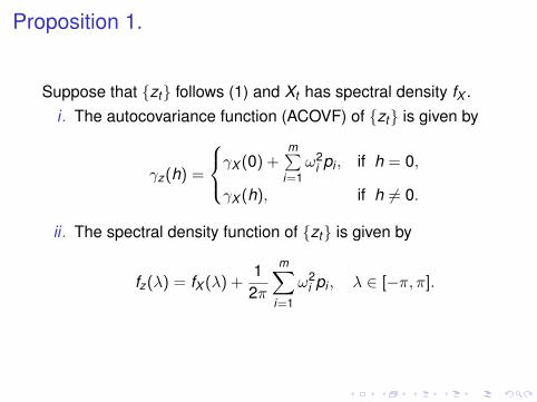
Proposition 1.
Suppose that {zt} follows (1) and Xt has spectral density fX .i . The autocovariance function (ACOVF) of {zt} is given by
γz(h) =
γX (0) +m∑
i=1ω2
i pi , if h = 0,
γX (h), if h 6= 0.
ii . The spectral density function of {zt} is given by
fz(λ) = fX (λ) +1
2π
m∑i=1
ω2i pi , λ ∈ [−π, π].

Proposition 2.
Let z1, z2, . . . , zn be a set of observations generated from model(1) with m = 1, and let the outlier occurs at time t = T . It followsthat:
i . The sample ACOVF is given by
γz(h) = γX (h)± ω
n(XT−h + XT+h − 2y) +
ω2
nδ(h) + op(n−1),
(2)
where γX (h) =1n
n−h∑t=1
(Xt − X )(Xt+h − X ) and
δ(h) =
{1, when h = 0,0, otherwise.

Proposition 2 (continuation).
ii . The periodogram is given by
Iz(λ) = IX (λ) + ∆(ω), [−π, π],
where
∆(ω) =ω2
2πn± ω
πn
{(XT − X ) +
n−1∑h=1
(XT−h + XT+h − 2X ) cos(hλ)
}(3)
+ op(n−1).

Proposition 3. (Chan (1992, 1995))
Suppose that z1, z2, . . . , zn is a set of observations generatedfrom model (1) and let ρz(h) = γz(h)/γz(0), then
i. For m = 1,
limn→∞
limω→∞
ρz(h) = 0.
ii. For m = 2 and T2 = T1 + l , such thath < T1 < T1 + l < n − h, we have
limn→∞
{plimω1→∞
ω2→±∞ρz(h)
}=
{0, if h 6= l ,±0.5, if h = l .

Some specific comments
I The outliers cause an increase in the variance of process,which reduces the magnitude of the autocorrelations andintroduces loss of information on the pattern of serialcorrelation.
I The spectral density of the process is characterized by antranslation due to the contributions of magnitude of outliers.
I These results also give the evidence that an outlier canseriously affect the autocorrelation structure due to anincrease in the variance.

Lemma 1.
Let {Xt}t∈Z be a stationary and invertible ARFIMA(p,d ,q) pro-cess. Also, let {zt}t∈Z be such that zt = Xt +
∑mi=1 ωi I
(T )t ,
where m is the number of outliers, the unknown parameter ωi
is the magnitude of the i th outlier at time Ti and I(Ti )t is Ber-
noulli distributed: Pr(
I(Ti )t = −1
)= Pr
(I(Ti )t = 1
)= pi
2 and
Pr(
I(Ti )t = 0
)= 1 − pi . The spectral density of {zt} is given
by
fz(λ) =σ2ε
2π|Θ(e−iλ)|2
|Φ(e−iλ)|2
{2 sin
(λ
2
)}−2d
+1
2π
m∑i=1
ω2i pi .
where λ ∈ [−π, π].
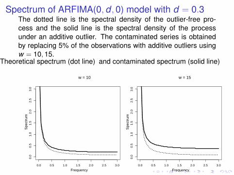
Spectrum of ARFIMA(0,d ,0) model with d = 0.3The dotted line is the spectral density of the outlier-free pro-cess and the solid line is the spectral density of the processunder an additive outlier. The contaminated series is obtainedby replacing 5% of the observations with additive outliers usingw = 10,15.
Theoretical spectrum (dot line)
0.0 0.5 1.0 1.5 2.0 2.5 3.0
0.0
0.5
1.0
1.5
2.0
2.5
3.0
w = 10
Frequency
Spe
ctru
m
and contaminated spectrum (solid line)
0.0 0.5 1.0 1.5 2.0 2.5 3.0
0.0
0.5
1.0
1.5
2.0
2.5
3.0
w = 15
Frequency
Spe
ctru
m

A robust estimator of ACF
Rousseeuw & Croux (1993) proposed a robust scale estimatorfunction which is based on the k th order statistic of
(n2
)distances
{|yi − yj |, i < j}, and can be written as
Qn(y) = c × {|yi − yj |; i < j}(k), (4)
where y = (y1, y2, . . . , yn)′, c is a constant used to guaran-tee consistency (c = 2.2191 for the normal distribution), and
k =
⌊(n
2)+24
⌋+ 1. The above function can be calculated using
the algorithm proposed by Croux & Rousseeuw (1992), which iscomputationally efficient. Rousseeuw & Croux (1993) showedthat the asymptotic breakdown point of Qn(·) is 50%, which me-ans that the time series can be contaminated by up to half ofthe observations with outliers and Qn(·) will still yield sensibleestimates.

A robust estimator of ACF- continuation
Q(·), Ma & Genton (2000) proposed a highly robust estimatorfor the ACOVF:
γ(h) =14
[Q2
n−h(u + v)−Q2n−h(u − v)
], (5)
where u and v are vectors containing the initial n − h and thefinal n − h observations, respectively. The robust estimator forthe autocorrelation function is
ρ(h) =Q2
n−h(u + v)−Q2n−h(u − v)
Q2n−h(u + v) + Q2
n−h(u − v).
It can be shown that |ρ(h)| ≤ 1 for all h.

ACF ARFIMA(0,d ,0) model, d = 0.3, n = 300
0 50 100 150 200 250 300
0.0
0.1
0.2
0.3
0.4
Outlier free−data
ACF (dot line)
Robust (dashed line)
Aut
ocov
aria
nces

ACF ARFIMA(0,d ,0) model, d = 0.3, n = 300
0 50 100 150 200 250 300
0.0
0.1
0.2
0.3
0.4
Data with outliers
ACF (dot line)
Robust (dashed line)
Aut
ocov
aria
nces

Theoretical Results-Short-memory and long-memorycases
It supposes that the empirical c.d.f. Fn, adequately normalized,converges. Let us first define the Influence Function. FollowingHuber (1981), the influence function x 7→ IF(x ,T ,F ) is definedfor a functional T at a distribution F at point x as the limit
IF(x ,T ,F ) = limε→0+
ε−1{T (F + ε(δx − F ))− T (F )} ,
where δx is the Dirac distribution at x . Influence functions are aclassical tool in robust statistics used to understand the effect ofa small contamination at the point x on the estimator.

Theoretical Results-Short-memory case
(Xi)i≥1 is a stationary mean-zero Gaussian process with auto-covariance sequence γ(h) = E(X1Xh+1) satisfying:∑
h≥1
|γ(h)| <∞ .

TheoremUnder some assumption Qn(X1:n) satisfies the following centrallimit theorem:
√n(Qn(X1:n)− σ)→ N (0, σ2) ,
where σ =√γ(0) and the limiting variance σ2 is given by
γ(0)E[IF2(X1/σ,Q,Φ)]+2γ(0)∑k≥1
E[IF(X1/σ,Q,Φ)IF(Xk+1/σ,Q,Φ)]
IF(·,Q,Φ) is the Influence Function defined previously.
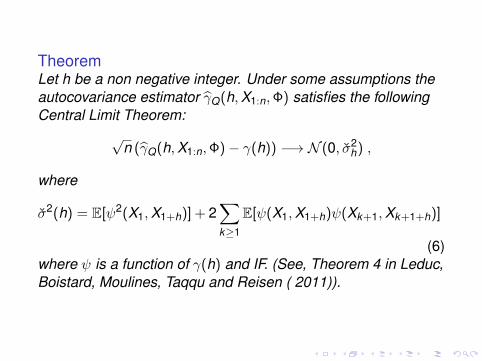
TheoremLet h be a non negative integer. Under some assumptions theautocovariance estimator γQ(h,X1:n,Φ) satisfies the followingCentral Limit Theorem:
√n (γQ(h,X1:n,Φ)− γ(h)) −→ N (0, σ2
h) ,
where
σ2(h) = E[ψ2(X1,X1+h)] + 2∑k≥1
E[ψ(X1,X1+h)ψ(Xk+1,Xk+1+h)]
(6)where ψ is a function of γ(h) and IF. (See, Theorem 4 in Leduc,Boistard, Moulines, Taqqu and Reisen ( 2011)).

Main theoretical Results-Long-memory case
Now, let (Xi)i≥1 be a stationary mean-zero Gaussian processwith autocovariance γ(h) = E(X1Xh+1) satisfying:
γ(h) = h−DL(h), 0 < D < 1 ,
where L is slowly varying at infinity and is positive for largeh.A classical model for long memory process is the so-calledARFIMA(p,d ,q), which is a natural generalization of standardARIMA(p,d ,q) models. By allowing d to assume any value in(−1/2,1/2). D = 1− 2d in above.
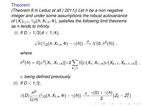
Theorem(Theorem 8 in Leduc et all ( 2011)) Let h be a non negativeinteger and under some assumptions the robust autovarianceof (Xi)i≥1, γQ(h,X1:n,Φ), satisfies the following limit theoremsas n tends to infinity.
(i) If D > 1/2(d < 1/4),
√n (γQ(h,X1:n,Φ)− γ(h))
d−→ N (0, σ2(h)) ,
where
σ2(h) = E[ψ2(X1,X1+h)]+2∑k≥1
E[ψ(X1,X1+h)ψ(Xk+1,Xk+1+h)] ,
ψ being defined previously.(ii) If D < 1/2,
β(D)nD
L(n)(γQ(h,X1:n,Φ)− γ(h))
d−→ γ(0) + γ(h)
2(Z2 − Z 2
1 )

In the theorem, β(D) = B((1 − D)/2,D), B denotes the Betafunction, the processes Z1,D(·) (the standard fractional Brownianmotion) and Z2,D(·) (the Rosenblatt process) are defined in theLevy-Leduc et al (2011), and
L(n) = 2L(n) + L(n + h)(1 + h/n)−D + L(n − h)(1− h/n)−D

PropositionUnder Assumption and D < 1/2 for the process (Xi)i≥1, therobust autocovariance estimator γQ(h,X1:n,Φ) has the sameasymptotic behavior as the classical autocovariance estimator.There is no loss of efficiency.
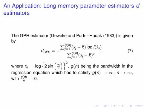
An Application: Long-memory parameter estimators-destimators
The GPH estimator (Geweke and Porter-Hudak (1983)) is givenby
dGPH = −∑g(n)
j=1 (xj − x) log I(λj)∑g(n)j=1 (xj − x)2
, (7)
where xj = log{
2 sin(λj2
)}2, g(n) being the bandwidth in the
regression equation which has to satisfy g(n) → ∞, n → ∞,with g(n)
n → 0.

The GPH estimator
Hurvich, Deo, Brodsky (1998) proved that, under some regula-rity conditions on the choice of the bandwidth, the GPH estima-tor is consistent for the memory parameter and is asymptoticallynormal when the time series is Gaussian. The authors also es-tablished that the optimal g(n) is of order o(n4/5). They showedthat if g(n) → ∞,n → ∞ with g(n)
n → 0 and g(n)n log g(n) → 0,
then, under some conditions on 0 < fu(λj) < ∞, the GPH esti-mator is a consistent estimator of d ∈ (−0.5,0.5) with variancevar(dGPH) = π2
24g(n) + o(g(n)−1).

A robust estimator of d
Assumption: Let M = min{h′,nβ} with 0 < β < 1, where
h′ = min{
0 < h < n : εtempn (γQ(h)) ≤ m
n
}− 1,
m and n are the numbers of outliers and the sample size, res-pectively.

A robust estimator of d
Let I(λ) be given by
I(λ) =1
2π
n−1∑s=−(n−1)
κ(s)R(s) cos(sλ), (8)
where R(s) is the sample autocovariance function in (5) andκ(s) is defined as
κ(s) =
{1, |s| ≤ M,
0, |s| > M.
κ(s) is called truncated periodogram lag window see, e.g., Pri-estley (1981, p. 433-437). We shall call the estimator in (8) ro-bust truncated pseudo-periodogram, since it does not have thesame finite-sample properties as the periodogram, with M = nβ,0 < β < 1.

A robust estimator of d
The robust GPH estimator we propose is
dGPHR = −∑g(n)
i=1 (xi − x) log I(λi)∑g(n)i=1 (xi − x)2
, (9)
where xi = log{
2 sin(λj2
)}2and g(n) is as before.

A robust estimator of dThe value of β, in M = nβ, was selected empirically by minimi-zing the MSE of the long-memory parameter estimates. TheFigure presents simulation results for a free-outliers ARFIMAprocess generated with n = 800 and 10000 Monte Carlo experi-
ments.

Numerical results: ARFIMA(0,d ,0) with d = 0.3
g(n) = n0.7 M = n0.7
d n dGPH dGPHc dGPHR dGPHR c
100 mean 0.2988 0.1134 0.2584 0.2449sd 0.1735 0.1619 0.1558 0.1556bias −0.0012 −0.1866 −0.0416 −0.0551MSE 0.0301 0.0610 0.0260 0.0272
300 mean 0.3062 0.1007 0.2907 0.28370.30 sd 0.1005 0.0978 0.0926 0.0960
bias 0.0062 −0.1993 −0.0093 −0.0163MSE 0.0101 0.0493 0.0087 0.0095
800 mean 0.3003 0.1184 0.2949 0.2869sd 0.0679 0.0715 0.0573 0.0610bias 0.0003 −0.1816 −0.0051 −0.0131MSE 0.0046 0.0381 0.0033 0.0039
ω = 10, outliers = 5% (of sample)

Numerical results: ARFIMA(0,d ,0) with d = 0.45
g(n) = n0.7 M = n0.7
d n dGPH dGPHc dGPHR dGPHR c
100 mean 0.4561 0.1923 0.3975 0.3778sd 0.1722 0.1727 0.1506 0.1433bias 0.0061 −0.2577 −0.0525 −0.0722MSE 0.0297 0.0962 0.0254 0.0258
300 mean 0.4594 0.2015 0.4329 0.42330.45 sd 0.0986 0.0976 0.1041 0.1013
bias 0.0094 −0.2485 −0.0171 −0.0267MSE 0.0098 0.0713 0.0111 0.0110
800 mean 0.4620 0.2306 0.4457 0.4349sd 0.0688 0.0809 0.0562 0.0576bias 0.0121 −0.2194 −0.0043 −0.0151MSE 0.0049 0.0547 0.0032 0.0035
ω = 10, outliers = 5% (of sample)

Numerical results: ARFIMA(0,d ,0) with d = 0.45
ω n dGPHc dGPHRc3 100 mean 0.3747 0.3799
sd 0.1953 0.1513bias −0.0753 −0.0701MSE 0.0438 0.0278
800 mean 0.4080 0.4309sd 0.0679 0.0576bias −0.0419 −0.0191MSE 0.0064 0.0037
5 100 mean 0.3108 0.3741sd 0.1934 0.1452bias −0.1392 −0.0759MSE 0.0567 0.0268
800 mean 0.3526 0.4270sd 0.0846 0.0568bias −0.0974 −0.0229MSE 0.0166 0.0038
10 100 mean 0.1923 0.3778sd 0.1727 0.1433bias −0.2577 −0.0722MSE 0.0962 0.0258
800 mean 0.2306 0.4349sd 0.0809 0.0576bias −0.2194 −0.0151MSE 0.0547 0.0035
outliers = 5% (of sample)

Numerical results: ARFIMA(0,d ,0) n = 300
GPH GPHR GPHc GPHRc
−0.
10.
00.
10.
20.
30.
40.
5

Numerical results: ARFIMA(0,d ,0) n = 3000
GPH GPHR GPHc GPHRc
0.1
0.2
0.3
0.4
Applications: Nile river 622 - 1281 D.C.
We have applied the methodology proposed in previous sectionto the annual minimum water levels of the Nile river measured atthe Roda Gorge near Cairo. This data set has been widely usedas to illustrate long-memory memory modeling strategies; seeBeran (1992), Reisen, Abraham & Toscano (2002), Robinson(1995), among others. The period analyzed ranges from 622A.D. to 1284 A.D. (663 observations).Various conclusions have been reached as to whether or notthis series contains outliers. For example, Chareka, Matarise &Turner(2006) developed a test to identify outliers and ran it onthe Nile data. Their test located two outliers at 646 A.D. and at809 A.D.

Applications: Nile river 622 - 1281 D.C.
622 722 822 922 1022 1122 1222
1000
1200
1400
0 10 20 30 40 50 60 70
−0.
10.
10.
30.
5
Lag
FA
C
0 10 20 30 40 50 60 70
−0.
10.
10.
30.
5
Lag
FA
CP
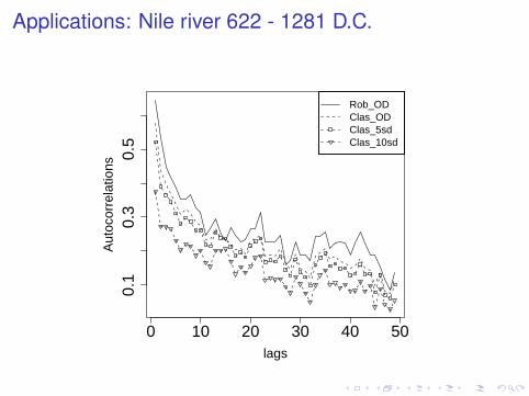
Applications: Nile river 622 - 1281 D.C.
0 10 20 30 40 50
0.1
0.3
0.5
lags
Aut
ocor
rela
tions
Rob_ODClas_ODClas_5sdClas_10sd

Applications: Nile river 622 - 1281 D.C.
GPH GPHRBandwidth d s.e. d s.e.g(n) = 25 0.503 0.142 0.459 0.057g(n) = 49 0.537 0.117 0.475 0.045g(n) = 94 0.396 0.079 0.416 0.040g(n) = 180 0.386 0.054 0.460 0.039
Tabela: Estimated values of d using the Nile data.
Based on a slight modification of the robust estimator proposedby Beran (1994), Agostinelli & Bisaglia (2004) found 0.412 asthe estimate of d which is very close to the GPHR estimate wheng(n) = 94.

Concluding remarks
The simulation results showed that the GPH estimator of thefractional differencing parameter can be considerably biased whenthe data contain atypical observations, and that the robust esti-mator we propose displays good finite-sample performance evenwhen the data contain highly atypical observations. Future re-search should address the important issue of establishing theasymptotic properties for the proposed estimator.

THANK YOU
References
Priestley, M.Spectral analysis and time series.Academic Press, 1983.
Agostinelli, C. & Bisaglia, L.Robust estimation of ARFIMA process.Technical Report Università Cà Foscari di Venezia, 2003.
Beran, J.On class of M-estimators for Gaussian long-memorymodels.Biometrika, 81:755-766, 1994.
References
Chan, W.A note on time series model specification in the presenceoutliers.Journal of Applied Statistics, 19:117–124, 1992.
Chan, W.Outliers and Financial Time Series Modelling: A CautionaryNote.Mathematics and Computers in Simulation, 39:425–430,1995.
Croux, C. & Rousseeaw P.Time-efficient algorithms for two highly robust estimators ofscale.Computational Statistics, 1:1–18, 1992.

References
Geweke, J. & Porter-Hudak, S.The estimation and application of long memory time seriesmodel.Journal of time serie analysis, 1:221–238, 1983.
Haldrup, N. & Nielsen, M.Estimation of fractional integration in the presence of datanoise.Computational statistical and data analysis, 51:3100-3114,2007.
Hosking, J.Fractional differencing.Biometrika, 68:165-176, 1981.

References
Hurvich C. M. & Beltaão K.Asymptotics for low-frequency ordinates of the periodogramof a long-memory time series.Journal of Time Series Analysis, 14:455–472, 1993.
Hurvich C. M., Deo R. & Brodsky J.The mean square error of Geweke and Porter-Hudak’sestimator of the memory parameter of a long-memory timeseries.Journal of Time Series Analysis, 19:19–46, 1998.
Künsch H. R.Discrimination between monotonic trends and long-rangedependence.Journal of Applied Probability, 23:1025–1030, 1989.
References
Ma, Y. & Genton, M.Highly robust estimation of the autocovariance function.Journal of time series analysis, 21:663–684, 2000.
Rousseeaw P. & Croux, C.Alternatives to the median absolute deviation.Journal of the American Statistical Association,88:1273–1283, 1993.


![Robust Model Predictive Control - Carnegie Mellon …cepac.cheme.cmu.edu/.../Ronust_Control_Classnotes.pdf1 Robust Model Predictive Control Formulations of robust control [1] The robust](https://static.documents.pub/doc/80x56/5aab45707f8b9a2b4c8bd345/robust-model-predictive-control-carnegie-mellon-cepacchemecmueduronustcontrol.jpg)
