Robust Inference of Risks of Large Portfolios · 2015-01-13 · Robust Inference of Risks of Large...

Robust Inference of Risks of Large Portfolios

Jianqing Fan∗, Fang Han†, Han Liu‡, and Byron Vickers §¶

January 10, 2015

Abstract

We propose a bootstrap-based robust high-confidence level upper bound (Robust

H-CLUB) for assessing the risks of large portfolios. The proposed approach exploits

rank-based and quantile-based estimators, and can be viewed as a robust extension of

the H-CLUB method (Fan et al., 2015). Such an extension allows us to handle possi-

bly misspecified models and heavy-tailed data. Under mixing conditions, we analyze

the proposed approach and demonstrate its advantage over the H-CLUB. We further

provide thorough numerical results to back up the developed theory. We also apply

the proposed method to analyze a stock market dataset.

Keywords: High dimensionality; robust inference; rank statistics; quantile statistics; risk

management; covariance matrix.

1 Introduction

Let R1, . . . ,RT be a stationary multivariate time series with Rt ∈ Rd representing the asset

returns at time t. Letting w ∈ Rd be a portfolio allocation vector, we define the risk of w as

Risk(w) := (Var(wTRt))1/2 = (wTΣw)1/2,

∗Department of Operations Research and Financial Engineering, Princeton University, Princeton, NJ

08544, USA; e-mail: [email protected]. His research is supported by NSF grant DMS-1406266 and

NIH grant R01GM100474-04.†Department of Biostatistics, Johns Hopkins University, Baltimore, MD 21205, USA; e-mail:

[email protected]. His research is supported by a Google fellowship.‡Department of Operations Research and Financial Engineering, Princeton University, Princeton, NJ

08544, USA; e-mail: [email protected]. His research is supported by NSF CAREER Award

DMS1454377, NSF IIS1408910, NSF IIS1332109, NIH R01MH102339, NIH R01GM083084, and NIH

R01HG06841.§Department of Operations Research and Financial Engineering, Princeton University, Princeton, NJ

08544, USA; e-mail: [email protected]. His research was supported by NIH 2R01-GM072611-10.¶We thank Huitong Qiu for discussions.

1

arX

iv:1

501.

0238

2v1

[m

ath.

ST]

10

Jan

2015

where Σ denotes the unknown volatility (or covariance) matrix of Rt. i.e.,

Σ := E[(Rt − ERt)(Rt − ERt)

T].

Assessing the risk of a portfolio includes two steps: First, we need a covariance matrix

estimator Σest; Secondly, we construct a confidence interval for wTΣw based on Σest.

Assessing the risk Risk(w) is challenging when d is large. For example, given a pool

of 2,000 candidate assets, the volatility matrix Σ involves more than 2 million parameters.

However, for daily returns data, the sample size is in general no larger than 500 over one and

a half years. This is a typical “small n, large d” problem which leads to the accumulation

of estimation errors (Jagannathan and Ma, 2003; Pesaran and Zaffaroni, 2008; Fan et al.,

2012). To handle the curse of dimensionality, more structural regularization is imposed

in estimating Σ. For example, Fan et al. (2008) and Fan et al. (2013) impose the factor

model structure on the covariance matrix. The assumed factor structure reduces the effective

number of parameters that have to be estimated. In addition, Ledoit and Wolf (2003) propose

a shrinkage estimator of Σ. Moreover, Barndorff-Nielsen (2002), Zhang et al. (2005), and Fan

et al. (2012) consider estimating Σ based on high-frequency data. Other literature includes

Chang and Tsay (2010), Gomez and Gallon (2011), Lai et al. (2011), Fan et al. (2011), Bai

and Liao (2012), and Fryzlewicz (2013).

However, most of these papers focus on risk estimation instead of uncertainty assessment.

To construct a confidence interval for wTΣw, Fan et al. (2012) propose to use ‖w‖21‖Σest −Σ‖max

1 as an upper bound of |wT(Σest−Σ)w|. However, this bound depends on the unknown

Σ and has proven to be overly conservative in numerical studies. To handle this problem,

Fan et al. (2015) further exploit several sample covariance based estimators Σest of Σ and

propose a high-confidence level upper bound (H-CLUB) of |wT(Σest − Σ)w|: For a given

confidence level 1−γ, under certain moment and dependence assumptions on the time series,

the derived H-CLUB proves to dominate |wT(Σest − Σ)w| with probability approximating

1− γ as both T and d increase to infinity.

This paper proposes new methods for uncertainty assessment of risks of large portfolios

for high dimensional heavy-tailed data. In particular, we derive confidence intervals for

wTΣw when the asset returns R1, . . . ,RT are elliptically distributed. This setting has

been commonly adopted in financial econometrics (Cont, 2001). To handle heavy-tailed

data, we propose a new risk uncertainty assessment method named robust high-confidence

level upper bound (Robust H-CLUB). The Robust H-CLUB exploits a new block-bootstrap-

based approach for uncertainty assessment of Risk(w). More specifically, we decompose the

problem of assessing the risk wTΣw into two parts: (i) We propose a robust estimator Σest

1We will provide the definitions of the vector `1 norm (‖ · ‖1) and matrix `max norm ‖ · ‖max later.

2

of Σ; (ii) We derive the variance of wT(Σest − Σ)w. For estimating Σ, we exploit rank-

based Kendall’s tau estimators and quantile-based median absolute deviation estimators. For

estimating the variance of wT(Σest −Σ)w, we employ the circular block bootstrap method

(Politis and Romano, 1992).

Theoretically, when T, d → ∞ and d is possibly much larger than T , we develop an

inferential theory of the robust risk estimators. In particular, we show that√TwT(Σest−Σ)w

is asymptotically normal with variance σ2, and the block-bootstrap-based estimator σ2est of σ2

is consistent. The theory holds even when d is nearly exponentially larger than T . Moreover,

it holds under any elliptical model. Thus we no longer need strong moment conditions (e.g.,

exponentially decaying rate on the tails of distributions) on the asset returns.

1.1 Other Related Work

There is a vast literature on estimating large sparse/factor-based covariance matrices. Under

the assumption that data points are mutually independent, many sample covariance based

regularization methods, including banding (Bickel and Levina, 2008b), tapering (Cai et al.,

2010), thresholding (Bickel and Levina, 2008a; Cai and Zhou, 2012), and factor structures

(Fan et al., 2008; Agarwal et al., 2012; Hsu et al., 2011), have been proposed. They are

further applied to study stationary time series data under vector autoregressive dependence

(Loh and Wainwright, 2012; Han and Liu, 2013c), mixing conditions (Pan and Yao, 2008;

Fan et al., 2011, 2013; Han and Liu, 2013b), and physical dependence (Xiao and Wu, 2012;

Chen et al., 2013).

This paper is also related to the literature on estimating large correlation/covariance

matrix under the misspecified or heavy-tailed model. For example, Han and Liu (2014b),

Han and Liu (2013a), Wegkamp and Zhao (2013), Mitra and Zhang (2014), and Fan et al.

(2014) exploit the rank statistics, while Qiu et al. (2014) focus on quantile statistics. None

of these works study the risk inference problem as in our paper.

1.2 Notation

Let v = (v1, . . . , vd)T be a d dimensional real vector and M = [Mjk] be a d by d real matrix.

For 0 < q < ∞, let the vector `q norm be ‖v‖q := (∑d

j=1 |vj|q)1/q and the vector `∞ norm

be ‖v‖∞ := maxdj=1 |vj|. For two subsets I, J ∈ 1, . . . , d, we denote vI and MI,J as the

sub-vector of v with entries indexed by I and sub-matrix of M with rows and columns

indexed by I and J . We denote the matrix `max norm of M as ‖M‖max := maxjk |Mjk|.Letting N = [Njk] ∈ Rd×d be another d by d real matrix, we denote by M N = [MjkNjk]

the Hadamard product between M and N. Letting f : R → R be a real function, we

denote by f(M) = [f(Mjk)] the matrix with f(Mjk) as its (j, k) entry. We write M =

3

diag(M1, . . . ,Mk) if M is block diagonal with diagonal matrices M1, . . . ,Mk. For random

vectorsX,Y ∈ Rd, we writeXd= Y ifX and Y are identically distributed. Throughout the

paper, we use c, c1, c2, . . . , and C,C1, C2, . . . to represent generic absolute positive constants,

for which the actual values may change at from one line to another. For any real positive

sequences an and bn, we write an & bn if we have an ≥ cbn for some absolute constant

c and all large enough n. We write an . bn if we have bn & an, and an bn if an . bn and

an & bn. For a ∈ R, we define dae and bac to be the smallest integer larger than a and the

largest integer smaller than a respectively.

1.3 Paper Organization

The rest of this paper is organized as follows. Section 2 introduces the Robust H-CLUB

estimator for assessing the uncertainty of the portfolio risk. We consider three settings: (i)

The marginal variances of the returns are known; (ii) The marginal variances are unknown,

but with additional information for helping determine the values; (iii) The marginal vari-

ances are unknown and there is no additional information available. Section 3 presents the

inferential theory for the risk estimators and justifies the use of Robust H-CLUB. Sections 4

and 5 present synthetic and real data analyses to back up the developed theory. Section 6

summarizes the results and discusses future work. Section 7 presents all the proofs.

2 Robust H-CLUB

This section introduces the Robust H-CLUB method. We consider a multivariate time

series of asset returns R1, . . . ,RT with Rt = (Rt1, . . . , Rtd)T ∈ Rd for t = 1, . . . , T . Let

Σ := Cov(Rt) be the covariance matrix and D ∈ Rd×d be a diagonal matrix with diagonals

Σ1/211 , . . . ,Σ

1/2dd . It is easy to derive Σ = DΣ0D, where Σ0 is the correlation matrix of Rt.

For a given portfolio allocation vector w ∈ Rd, we aim to construct a confidence interval for

wTΣw. Throughout this section, our interest is on analyzing heavy-tailed returns, which

are common in financial applications.

We exploit the elliptical distribution family to model heavy-tailed data. The ellipti-

cal distribution is routinely used in modeling financial data (Owen and Rabinovitch, 1983;

Hamada and Valdez, 2004; Frahm and Jaekel, 2007). More specifically, a random vector

Z ∈ Rd follows an elliptical distribution with mean µ ∈ Rd and positive definite covariance

matrix Σ ∈ Rd×d if

Zd= µ+ ξAU ,

where A ∈ Rd×d satisfies AAT = Σ, U ∈ Rd is uniformly distributed on the d-dimensional

sphere Sd−1, and ξ is an unspecified nonnegative random variable independent of U satisfying

4

Eξ2 = d. We impose the following stationary assumption on RtTt=1:

• (A0). R1, . . . ,RT are continuous and identically distributed as an elliptical random

vector R with covariance and correlation matrices Σ and Σ0.

For parameter estimation, we define the rank-based Kendall’s tau correlation coefficient

and quantile-based median absolute deviation estimators. In detail, given R1, . . . ,RT , the

sample and population Kendall’s tau matrices T = [τjk] and T = [τjk] are defined as

τjk :=2

T (T − 1)

∑

t<t′

sign(Rtj −Rt′j)sign(Rtk −Rt′k),

τjk := Esign(Rj − Rj)sign(Rk − Rk), (2.1)

where R = (R1, . . . , Rd)T and R = (R1, . . . , Rd)

T are two independent copies of R1. Under

the elliptical model, the Kendall’s tau matrix T and correlation matrix Σ0 satisfy (Lindskog

et al., 2003):

Σ0jk = sin

(π2τjk

). (2.2)

Next, we define the quantile-based median absolute deviation estimator of the scale

parameter. We start with some extra notation. Let X ∈ R be a random variable and

X1, . . . , XT be T realizations of X. For any q ∈ [0, 1], we define the population and

sample q-quantiles as

Q(X; q) := infx : P(X ≤ x) ≥ q

,

Q(Xt; q) := X(k), where k = mint :

t

T≥ q. (2.3)

Here X(1) ≤ X(2) ≤ · · · ≤ X(T ) are the ordered sequence of X1, . . . , XT2. We then define

the population and sample median absolute deviations for X1, . . . , XT as the population

and sample medians of absolute values of the centered data. The formal definitions are as

follows:

σM(X) := Q(∣∣∣X −Q

(X;

1

2

)∣∣∣

;1

2

),

σM(XtTt=1) := Q(∣∣∣Xt − Q

(XtTt=1;

1

2

)∣∣∣Tt=1

;1

2

). (2.4)

They are robust alternatives to the population and sample standard deviations. In particular,

for an elliptically distributed random vector R = (R1, . . . , Rd)T, Han et al. (2014) prove that

σM(R1)

sd(R1)=σM(R2)

sd(R2)= · · · = σM(Rd)

sd(Rd), (2.5)

2Let F and f be the distribution function and density function of X. We will use Q(X; q), Q(F ; q), and

Q(f ; q) exchangeably.

5

where for arbitrary random variable X, sd(X) represents the standard deviation of X.

Under the elliptical model and using the rank- and quantile-based estimators, we propose

three robust approaches to construct the confidence interval of wTΣw. Formally speaking,

for each proposed robust covariance matrix estimator Σest and any given γ > 0, we aim to

find a Uest(γ) such that

P(wTΣw ∈

[wTΣestw − Uest(γ),wTΣestw + Uest(γ)

])→ 1− γ,

as T, d→∞. The proposed approaches correspond to three scenarios where D has different

structures.

Of note, a main strategy throughout the proposed three methods is to separately estimate

the marginal standard deviations and bivariate correlation coefficients. In this paper, we

focus on measuring the uncertainty introduced in estimating the correlation coefficients,

while assuming that the uncertainty introduced in estimating marginal standard deviations

is negligible3. For measuring the uncertainty in correlation coefficients estimation, we employ

a circular block bootstrap method.

In detail, suppose that we derive robust marginal standard deviation estimator Dest of

D. We further derive the correlation matrix estimator Σ0est of Σ0 based on a d-dimensional

multivariate time series X1, . . . ,XT . For any given portfolio allocation vector w, we propose

to estimate wTΣw by

Risk(w) := wTΣestw, where Σest := DestΣ0estDest. (2.6)

To estimate the asymptotic variance of the estimator wTΣestw, we adopt a circular block

bootstrap procedure introduced in Politis and Romano (1992). First, we extend the sample

X1, . . . ,XT periodically by concatenating Xi+T = Xi for i ≥ 1. We then randomly select

a block of l = lT T 1−ε0 consecutive observations from the extended sample for some

absolute constant ε0 < 1 (e.g., we can pick ε0 to be 0.9). As the financial time series admits

weakly dependence structure, the choice of block size l is not very important. We repeat

this process b = bT/lc times independently to obtain a sample X∗1 , . . . ,X∗T , so that for each

k = 0, . . . , b− 1,

P∗(X∗kl+1 = Xj, . . . ,X

∗(k+1)l = Xj+l−1

)= 1/T, for j = 1, . . . , T,

where P∗ is the resampling distribution conditional on X1, . . . ,XT . Based on each re-

sampled time series X∗1 , . . . ,X∗T , we calculate the correlation matrix estimator Σ0∗

est. Let

Σ∗est := DestΣ0∗estDest be the estimator of Σ based on the resampled data and Var∗(·) be the

3This is mainly for the purpose of constructing the bootstrap-based inferential theory.

6

variance operator of the probability mass function P∗. We estimate the asymptotic variance

of wTΣestw by

σ2est := Var∗(

√TwTΣ∗estw).

2.1 Known Marginal Volatilities

In this section we consider the setting where the marginal standard deviations ofRt, encoded

in D, are known. While this is an ideal assumption, a practical implementation is to fit a

parametric model such as the GARCH(1,1) model introduced in Bollerslev (1986) to each

individual return time series. Such estimates are much more accurate than the nonparametric

ones and can be ideally treated as known.

When D is known, estimating wTΣw reduces to estimating the correlation matrix Σ0.

Using (2.2), under the elliptical model, we focus on the covariance matrix estimator Σ with

Σ := D sin(πT/2

)D. We then estimate wTΣw via replacing Σest by Σ in (2.6). Let σ2 be

an estimator of the asymptotic variance σ2 of wTΣw. We calculate σ2 based on the circular

block bootstrap method introduced earlier. Let Φ(·) be the cumulative distribution function

of a standard Gaussian random variable. For any given confidence level 1 − γ ∈ (0, 1), we

define the Robust H-CLUB estimator U(γ) as

U(γ) := Φ−1(1− γ/2)√σ2/T . (2.7)

The corresponding confidence interval for the risk is

[wTΣw − U(γ),wTΣw + U(γ)

]. (2.8)

In Section 3 we will show that, under mild conditions,

σ2 = σ2(1 + oP (1)) and P|wT(Σ−Σ)w| ≤ Uτ (γ)

→ 1− γ,

as T and d go to infinity. Therefore [wTΣw−U(γ),wTΣw+U(γ)] is a valid level (1−γ)100%

interval covering the true wTΣw.

2.2 Additional Data

This section considers the setting that there are available historical data for estimating D.

To adapt to the current market condition, we usually pick a short time series such that the

asset returns are approximately stationary. However, it is likely that each univariate time

series is stationary over a longer time scale than the multivariate time series, and hence we

can incorporate extra information into calculation of the marginal standard deviations.

7

Inspired by this, we consider a setting where historical information is available. We do not

assume the historical data to be multivariately stationary, but only marginally stationary.

Formally speaking, let R1, . . . ,RT be the observed stationary multivariate time series, and

H1, . . . ,HTh be the available historical data with Ht = (Ht1, . . . , Htd)T and

T = O(T 1−δh ), where δ is an absolute constant. (2.9)

H1, . . . ,HTh could have overlap with R1, . . . ,RT . However, Ht is not necessarily identically

distributed to either Ht′ or R1 for any t 6= t′ ∈ 1, . . . , Th. Instead, we only assume that

H1jd= H2j

d= · · · d

= HThj and Var(H1j) = Var(R1j), for j ∈ 1, . . . , d.

We then estimate wTΣw by separately estimating D and Σ0.

Formally, for estimating D, we use the historical data H1, . . . ,HTh and derive

Dh = (Dh11, . . . , D

hdd), where Dh

jj := σhM,jσh1σhM,1

, (2.10)

and σhM,j = σM(HtjTt=1), for j = 1, . . . , d, is the median absolute deviation estimator of

HtjTt=1, and σh1 =(Var(Ht1Tt=1)

)1/2is the Pearson sample standard deviation of Ht1Tt=1.

For estimating Σ0, we calculate the Kendall’s tau matrix T based on R1, . . . ,RT.Remark 2.1. In (2.10), to calculate Dh, we employ the term σh1/σ

hM,1 to approximate the

scaling factor between the median absolute deviation and the Pearson’s standard deviation.

This facilitates theoretical derivations. In practice, we can use, for example, the average

version∑d

j=1 σhj /∑d

j=1 σhM,j to estimate the scaling factor.

For estimating wTΣw, we replace Dest by Dh, Σ0est by sin(πT/2), and Σest by Σh in

(2.6). For any given 1− γ ∈ (0, 1), we calculate the Robust H-CLUB estimator Uh(γ) as

Uh(γ) = Φ−1(1− γ/2)√σ2h/T , (2.11)

where σ2h is calculated by employing the circular block bootstrap method introduced earlier.

The corresponding confidence interval for the risk is[wTΣhw − Uh(γ),wTΣhw + Uh(γ)

]. (2.12)

2.3 Unknown Marginal Volatilities

This section considers the setting that D is unknown with no additional data available.

More precisely, we use a data splitting strategy for separately estimating D and Σ0. More

precisely, we estimate D using the whole dataset:

D = (D11, . . . , Ddd), with Djj := σM,jσ1σM,1

, (2.13)

8

where σM,j = σM(RtjTt=1) for j = 1, . . . , d and σ1 =(Var(Rt1Tt=1)

)1/2is the Pear-

son sample standard deviation of Rt1Tt=1. For estimating Σ0, we extract a subsequence

RT−Ts+1, . . . ,RT from the time series R1, . . . ,RT , where Ts T 1−δ with δ a small enough

absolute constant. Using this subsequence, we calculate the Kendall’s matrix Ts. Combining

it with D, we obtain a robust covariance matrix estimator

Σs := D sin(π

2Ts)

D.

We then estimate wTΣw via replacing Dest, Σ0est, and Σest by D, sin(π

2Ts), and Σs in (2.6).

We then obtain a Robust H-CLUB estimator as

U s(γ) = Φ−1(1− γ/2)√σ2s/Ts, (2.14)

where σ2s is calculated by employing the circular block bootstrap method. Accordingly, we

construct the confidence interval of the risk as

[wTΣsw − U s(γ),wTΣsw + U s(γ)

]. (2.15)

Remark 2.2. In (2.13), for estimating the scaling factor, we can employ a similar average

version as in Remark 2.1. We also note that the data splitting strategy is mainly proposed for

theoretical analysis. In practice, we can set δ = 0 and use the entire data set in calculating

Σs and performing the block bootstrap.

3 Asymptotic Theory

In this section we prove that the confidence intervals of wTΣw corresponding to three settings

discussed in Section 2 have desired coverage probability. In other words, we prove that the

Robust H-CLUB estimators proposed in (2.7), (2.11), and (2.14) are asymptotic (1−γ)100%

confidence upper bound for the risk. It is clear that this problem reduces to calculating the

limiting distributions of wT(Σest −Σ)w for Σest = Σ, Σh, and Σs. In the sequel, we adopt

the triangular array setting as in Fan and Peng (2004) and Greenshtein and Ritov (2004)

and allow the dimension d to increase with the sample size n.

We introduce several mixing conditions for measuring degree of dependence. We start

with an introduction of three mixing coefficients. For a d-dimensional stationary process

Rtt∈Z, let F ba be the σ-algebra generated by Ra, . . . ,Rb for a ≤ b. We define the α-, β-,

9

and φ-mixing coefficients as follows:

α(n) := supB∈F0

−∞,A∈F∞n

∣∣P(A ∩B)− P(A)P(B)∣∣,

β(n) := E

supA∈F∞n

∣∣P(A|F0−∞)− P(A)

∣∣,

φ(n) := supB∈F0

−∞,A∈F∞n ,P(B)>0

∣∣P(A|B)− P(A)∣∣.

For an arbitrary positive integer n, we have α(n) ≤ β(n) ≤ φ(n) (Yoshihara, 1976).

Suppose that R1, . . . ,RT is a subsequence of the stationary process Rtt∈Z. Let F

be the distribution function of R1. For a := Dw = (a1, . . . , ad)T, let g : Rd × Rd → R be a

kernel function

g(Rt,Rt′) :=π

2

∑

j 6=kajak cos(

π

2τjk)sign(Rtj −Rt′j)sign(Rtk −Rt′k). (3.1)

We further define the following 3 quantities which will be useful in the later sections:

g1(R1) :=

∫g(R1,R2)dF (R2), (3.2)

θ :=

∫g(R1,R2)dF (R1)dF (R2) = aT

cos(

π

2T) π

2Ta, (3.3)

σ2 := 4(Eg1(R1)

2 − θ2 + 2∞∑

h=1

Eg1(R1)g1(R1+h)

). (3.4)

In the following, we assume that the elliptical time series model in Section 2 holds.

3.1 Theory for Known Volatilities

We make the following four assumptions which regulate the portfolio allocation vector w

and the stationary process Rtt∈Z.

(A1) There exist absolute constants C1 and C2 such that ‖w‖1≤C1 and ‖Σ‖max≤C2.

(A2) σ is lower bounded by a positive absolute constant.

(A3) The process Rtt∈Z is φ-mixing with φ(n) ≤ n−1−ε for some ε > 0.

(A4) log d/(T 1/2) = o(1).

Assumption (A1) regulates the portfolio allocation vector w to prevent extreme positions.

It is a common assumption made for stability of the portfolio (Jagannathan and Ma, 2003;

10

Fan et al., 2012, 2015). Assumption (A2) guarantees that the portfolio risk can not be

diversified away. This is mild given that the returns are commonly assumed to follow a

factor model (Chamberlain, 1983; Fan et al., 2015). Assumption (A3) is routinely used in

analyzing time series to capture the serial dependence strength (Pan and Yao, 2008; Han

and Liu, 2013b). Lastly, Assumption (A4) allows d to grow nearly exponentially faster than

T and hence is mild.

In the setting of Section 2.1 and Assumptions (A1)-(A4), we derive the limiting distribu-

tion of wT(Σ−Σ)w. The following theorem shows that√TwT(Σ−Σ)w/σ is asymptotically

normal.

Theorem 3.1 (CLT, known volatilities). Assuming that (A0) - (A4) hold and in the setting

of Section 2.1, we have

√TwT(Σ−Σ)w/σ

d→ N(0, 1),

as both T and d go to infinity.

The following theorem verifies that σ2 calculated using the circular block bootstrap ap-

proach is a consistent estimator of σ2. This result, combined with Theorem 3.1 and Slutsky’s

theorem, confirms that√TwT(Σ−Σ)w/σ converges weakly to the standard Gaussian. Ac-

cordingly, the confidence interval in (2.8) gives a reliable coverage probaility.

Theorem 3.2 (bootstrap, known volatilities). Under Assumptions (A0) - (A4), we have

σ2 = σ2(1 + oP (1)

),

and accordingly, for any given γ ∈ (0, 1), as T, d→∞, we have

P(wTΣw ∈

[wTΣw − U(γ),wTΣw + U(γ)

])→ 1− γ.

The above two theorems only assume that the marginal second moments exist. Therefore,

the Robust H-CLUB estimator naturally handles heavy-tailed data.

3.2 Theory with Additional Data

In this section we study the setting in Section 2.2. When D is unknown, we require additional

assumptions. First, the following three assumptions require that d does not grow too fast

compared to n and the given time series Xtt∈Z (either Rtt∈Z or Htt∈Z) is φ-mixing

with an exponentially decaying serial dependence.

• (A5). max√

log d/T δ, log d/(T 1/2) = o(1).

11

• (A6). The process Xtt∈Z is φ-mixing with φ(n) ≤ C1 exp(−C2nr) for some absolute

constants C1, C2, r > 0.

• (A7). Letting a = max(1, 1/r), we require that log d = o(T 1/(2a+3)).

Recall that δ is defined in (2.9) for characterizing the length of historical data. Secondly, we

require that the returns’ (4 + ε1)-th moments exist for some absolute constant ε1 > 0, and

the density functions are bounded away from zero around the median:

• (A8). For any j ∈ 1, . . . , d, E|X1j|4+ε1 ≤ C0 <∞ for some constant ε1, C0 > 0.

• (A9). Let fj and fj be the density functions of Xj and |Xj − Q(Xj; 1/2)|. For any

j ∈ 1, . . . , d, we require inf |x−Q(f ;1/2)|<κ f(x) ≥ η for some positive absolute constants

κ and η, and any f ∈ fj, fj.

Under (A0) - (A2) and (A5) - (A9), the next theorem shows that√TwT(Σh − Σ)w is

asymptotically normal.

Theorem 3.3 (CLT, unknown volatilities with additional data). Assume that Assumptions

(A0) - (A2) hold. In addition, assume that Assumptions (A5) - (A7) hold for both Rtt∈Zand the additional data Htt∈Z, and Assumptions (A8) - (A9) hold for Htt∈Z. Then in

the setting of Section 2.2, we have

√TwT(Σh −Σ)w/σ

d→ N(0, 1),

as both T and d go to infinity.

The next theorem shows that σ2h is a consistent estimator of σ2 and accordingly the

confidence interval in (2.12) is valid.

Theorem 3.4 (bootstrap, unknown volatilities with additional data). Under the assump-

tions of Theorem 3.3, we have

σ2h = σ21 + oP (1),


P(wTΣw ∈

[wTΣhw − Uh(γ),wTΣhw + Uh(γ)

])→ 1− γ.

12

3.3 Theory with Unknown Marginal Volatilities

Lastly we study the setting in Section 2.3. Under this setting, we use a data splitting strategy

and make inference only on a subsequence of length T 1−δ. The next theorem justifies the

use of such an approach.

Theorem 3.5 (CLT, unknown marginal volatilities). Assume that Assumptions (A0) -

(A2) hold and Assumptions (A5) - (A9) hold for Rtt∈Z. Then, under the setting of

Section 2.3, we have√Tsw

T(Σs −Σ)w/σd→ N(0, 1).

Furthermore, the bootstrap-based estimator σ2s proves to be a consistent estimator of σ2.

Theorem 3.6 (bootstrap, unknown marginal volatilities). Under the assumptions of Theo-

rem 3.5, we have

σ2s = σ21 + oP (1),


P(wTΣw ∈

[wTΣsw − U s(γ),wTΣsw + U s(γ)

])→ 1− γ.

Remark 3.7. Compared to the method in Fan et al. (2015), the Robust H-CLUB estimator

gains substantial robustness since it only assumes that the (4 + ε1)-th moments exist for the

marginal returns. In comparison, Fan et al. (2015) require a strong exponentially decaying

rate in the tails (Check, for example, Assumption 3.4 therein). Such assumptions are often

too restrictive and rarely satisfied in real applications. The Robust H-CLUB estimator

attains the power for handling heavy-tailed data at the cost of a small T δ efficiency. This is

due to the data splitting strategy, which is an artifact of the proof. In practice, we find that

the method introduced in Section 2.3 performs well.

The data splitting strategy allows the portfolio allocation vector to be random. More

specifically, suppose that w is calculated based on the data R1, . . . ,RT . The next theorem

shows that√Tsw

T(Σs −Σ)w is asymptotically normal under assumptions outlined below.

Corollary 3.1. Under the assumptions in Theorem 3.5, let w = (w1, . . . , wd)T be an esti-

mator of w = (w1, . . . , wd)T satisfying that

P(|wj/wj − 1| > t) ≤ 2 exp(−CTt2

)(3.5)

for some absolute constant C, any j ∈ 1, . . . , d, and any t > 0. We then have, as T, d→∞,√Tsw

T(Σs −Σ)w/σd→ N(0, 1).

In this case, we can also employ a similar circular block bootstrap procedure for estimating

the asymptotic variance of√Tsw

T(Σs −Σ)w.

13

4 Simulations on Synthetic Data

In this section we examine the finite-sample performance of the Robust H-CLUB estimators

on synthetically generated data with heavy tails and noise contamination. We calculate sev-

eral statistics of the estimators, following those used in Fan et al. (2015), to show the quality

of the estimators. Our analysis shows that the Robust H-CLUB estimator performs well in all

of the cases considered when compared to the full-confidence bound ξT = ‖w‖21‖Σest−Σ‖max.

We observe that 95% confidence intervals by our proposed method are much tighter than

the bound given by ξT . We also demonstrate that the H-CLUB calculated based on the

robust estimators outperforms the H-CLUB based on the sample covariance matrix esti-

mator S proposed in Fan et al. (2012) in the presence of heavy-tailed data. In particular,

we show that the H-CLUB estimator does not achieve coverage proportions of 95% in the

heavy-tailed setting, while the performance of the Robust H-CLUB estimator is consistently

reliable. Lastly, we show that the Robust H-CLUB estimators also perform competitively

when applied to the Gaussian data.

4.1 Calibration and Parameter Selection

To calibrate the parameters governing data generation in our model, we use the daily re-

turns of the S&P 500’s top 100 stocks ranked by market capitalization (as of June 29th,

2012), and the 3-month Treasury bill rates, sourced from the COMPUSTAT database

(www.compustat.com) and the CSRP database (www.crsp.com), respectively. We consider

the excess returns yt over the period from July 1, 2008 to June 29, 2012. We extract the

following features:

1. d†i100i=1 with d†i equal to the sample standard deviation of the i-th stock.

2. Σ0† = Σ0†ij 100i,j=1, the sample correlation matrix of the observations yt.

From these, we extract the mean and variance of d†i100i=1, denoted respectively by µd† and

σ2d† . We also compute the average and standard deviation of all pairwise correlations, denoted

respectively by µΣ0† and σ2Σ0† . These parameters are used to generate correlation matrices

and marginal variances later on.

We also have several tuning parameters to select. We choose Th = dT 1/(1−δh)e with δh =

0.1 as the parameter determining the quantity of historical data available to the estimator Σh,

l = bT 1−ε0c with ε0 = 0.8 as the parameter controlling the block size in the block bootstrap,

Nbootstrap = 50 as the number of bootstrapped datasets generated, and Ts = bT 1−δc with

δ = 0.01 as the parameter controlling the data-splitting used in the estimator Σs.

14

4.2 Simulation

For each given gross exposure constraint c := ‖w‖1, we set T = 300 and allow d to range

from 50 to 500 in multiples of 50. For each value of d we conduct 200 iterations of the same

procedure: Generate a model, synthesize data from that model, and then calculate estimates

based on the synthesized data. We collate the outputs across these 200 iterations to allow

us to compare performance between different estimators.

The detailed procedure is described as follows:

1. Generate didi=1 independently from the Gamma distribution with mean µd† and vari-

ance σ2d† . Define D as the diagonal matrix such that Dii = di.

2. Generate entries Σiji 6=j of Σ0 independently from the Gaussian distribution with

mean µΣ0† and variance σ2Σ0† . We threshold these off-diagonal elements to be no

greater than 0.95 and set the diagonals of Σ0 to be 1. If the matrix is not positive

definite, we use Higham’s algorithm (see, e.g. Higham (2002)) to make it so, while

keeping the diagonals fixed at 1.

3. Define the covariance matrix Σ = DΣ0D.

4. Generate RtTt=1 independently from the multivariate t distribution with 5 degrees of

freedom and covariance matrix Σ. Generate independent historical data HtTht=1 from

the multivariate t distribution with 5 degrees of freedom and covariance matrix D2.

5. Add noise contamination to the data by selecting a random 1% of the elements in

RtTt=1 and multiplying each one by a random variable drawn independently from a

Unif(1, 15) distribution. Do the same to 1% of the elements in HtTht=1. This step can

be regarded as the news arrivals on the firms that cause their returns to jump.

6. Calculate the covariance estimates given by the sample covariance matrix S and the

robust estimators Σ, Σh, and Σs, using the tuning parameters given in Section 4.14.

7. Generate 500 portfolio allocation vectors w according to the method outlined in Fan

et al. (2015), which is approximately uniformly distributed on the manifold w :

‖w‖1 = c,wT1 = 1.4We find the following minor alteration to improve performance in practice: For the H-CLUB based on Σh,

we take block-bootstrapped samples of both HtTht=1 and RtTt=1 in estimating the variance of wTΣhw.

For this we use the block size parameter lh = bT 1−ε0h c, entirely analogously to the block bootstrapping

performed on RtTt=1 with l = bT 1−ε0c. We use this modification throughout Sections 4 and 5.

15

8. For each portfolio allocation, calculate the H-CLUB estimates corresponding to the

estimators listed in Step 6. As proof-of-concept, we also calculate the estimator with

ΣsTs=T

, which is the estimator Σs with Ts = T (i.e., no data-splitting performed).

9. Over the 500 portfolios, compute the averages of the true risk R(w) :=√

wTΣw, as

well as ∆ := |wT(Σest −Σ)w|, ξT := ‖w‖21‖Σest −Σ‖max, and U(0.05) = 2√σ2/T for

each of the estimators Σest considered.

We plot the averages of ∆, ξT , and U(0.05) against d for every estimator considered and for

c = 1, c = 1.6, and c = 2 to observe the effects of gross exposure on risk assessment.

Next, for d = 200 and d = 500, we calculate the following quantities over the 100,000

portfolios (500 portfolios over 200 synthetic datasets) : The coverage proportion, defined

as the fraction of the sample in which the 95% confidence interval contains the true risk

R(w) = (wTΣw)1/2, the ratio of bounds defined as

RE1 :=ξT

2√σ2/T

,

and the relative error defined as

RE2 :=

√σ2/T

2wTΣw.

Again, we compute these for c = 1, 1.6, and 2. The measure RE1 compares the upper bound

with the half width of the 95% confidence interval, whereas RE2 is the half width of 95%

confidence interval for the portfolio risk wTΣw1/2 divided by the portfolio risk itself. The

former depicts how inefficiency the confidence upper bound is and the latter measures how

informative the constructed confidence interval is.

Lastly, we repeat the previous calculations of coverage proportions, RE1 and RE2 in

a setting where the data are generated from a Gaussian distribution without any noise

contamination. This means we alter Step 4 of the procedure above (but substitute Gaussian

distribution for t distribution) and remove Step 5. This allows us to examine the degree

of efficiency loss for robustness when data are normal. In this setting, we also calculate

the ratio U(0.05)/∆ as a measure of how tight the H-CLUB is relative to the theoretical

minimum bound.

4.3 Results

In Figures 1 and 2, we plot the average risk estimation errors along with the estimated error

bounds with gross exposure c = 1, 1.6, and 2, using estimators Σest = Σ, Σh, Σs, and ΣsTs=T

.

Note that c = 1.6 results in an average 130% long positions and 30% short positions, which

16

100 200 300 400 500

010

0025

00

Sample covariance estimator

d

100 200 300 400 500

020

40

Robust estimator

d100 200 300 400 500

020

40

Robust estimator (no data−splitting)

d

100 200 300 400 500

020

40

Robust estimator (known history)

d100 200 300 400 500

0.0

1.5

3.0

Robust estimator (known marginal variance)

d

Figure 1: Averages of ∆ = |wT(Σest − Σ)w| (blue curve), U(0.05) = 2

√Var(wTΣestw)

(dashed curve), and ξT = ‖w‖21‖Σest −Σ‖max (red curve) for c = 1.0. Horizontal axis shows

dimension of problem, i.e., portfolio size. Vertical axis shows the calculated averaged values.

is commonly used in practice. We also use the sample covariance matrix estimator S, for

which an H-CLUB estimator was derived in Fan et al. (2015), which is not robustified.

From these plots, we see that

• The dashed curve lies above the solid blue line throughout, an indication of the validity

of the 95% bound given by U(0.05). It is interesting to note that this still holds for

the sample covariance matrix estimator S, but this is in the average sense. As we will

see in Table 1, however, S fails to attain 95% coverage.

• The crude bound ξT is much larger than either the true error ∆ or the 95% confidence

bound U(0.05). This discrepancy increases with d, but also with c as we can see by

comparing Figure 1 with Figure 2. This is quantified in Table 2.

• For large d the crude bound on the sample covariance matrix estimator is almost 100

times larger than on any of the robust estimators. This suggests inaccurate estimation

of the sample covariance in the presence of heavy tails and contamination.

Table 1 illustrates the coverage of each estimator, defined as the proportion of samples

in which the 95% confidence interval captures the true variance wTΣw. It can be seen that

all the robust estimators have coverage proportions of approximately 95%. However, the

17

100 200 300 400 500

030

00Sample covariance estimator

d

100 200 300 400 500

060

140 Robust estimator

d

100 200 300 400 500

060

140 Robust estimator (no data−splitting)

d

100 200 300 400 500

060

120


d

100 200 300 400 500

04

8


d

(a) c = 1.6

100 200 300 400 500

060

00

Sample covariance estimator

d

100 200 300 400 500

010

0

Robust estimator

d

100 200 300 400 500

010

0

Robust estimator (no data−splitting)

d

100 200 300 400 500

010

0


d

100 200 300 400 500

04

814


d

(b) c = 2

Figure 2: Averages of ∆ = |wT(Σest − Σ)w| (blue curve), U(0.05) = 2

√Var(wTΣestw)

(dashed curve) and ξT = ‖w‖21‖Σest −Σ‖max (red curve) for c = 1.6 and c = 2. Horizontal

axis shows dimension of problem, i.e., portfolio size. Vertical axis shows the calculated

averaged values.

sample covariance matrix estimator S has substantially lower coverage. It is not sufficiently

robust to give a valid bound under the current setting.

We make further comparisons between the robust estimators we have proposed. Table 2

illustrates averages and standard deviations of the ratio RE1 = ξT/U(0.05): the ratio between

the full confidence bound and the H-CLUB. These serve to quantify some of our observations

made on Figures 1 and 2 — in particular, that the ratio ξT/U(0.05) increases strongly with

c and weakly with d.

We observe that:

• The value of RE1 is considerably bigger than 1, reflecting the fact that the confidence

interval given by the Robust H-CLUB is much tighter than that given by the crude

bound. In almost all cases the value of RE1 reflects a difference of scale of an order of

magnitude between the H-CLUB interval and the crude interval using ξT .

18

Table 1: Empirical coverage proportion for 95% confidence intervals in settings of data drawn

from t5 distribution with 1% noise contamination. Taken over 200 samples with T = 300.d = 200 d = 500

c = 1.0 c = 1.6 c = 2.0 c = 1.0 c = 1.6 c = 2.0

Coverage81.88% 72.29% 69.31% 83.30% 82.24% 80.12%

S

Coverage97.59% 95.26% 97.64% 99.00% 97.09% 95.52%

Σs

Coverage96.38% 95.70% 97.49% 98.18% 97.03% 95.03%

ΣsTs=T

Coverage93.87% 93.19% 95.23% 93.01% 92.84% 94.67%

Σh

Coverage94.21% 95.54% 96.40% 95.16% 93.41% 93.67%

Σ

• The ratio RE1 increases with our ability to accurately estimate the marginal stan-

dard deviations. Note that RE1(Σ) > RE1(Σh) > RE1(Σ

sTs=T

) > RE1(Σs), which

corresponds to an ordering based on the amount of information used to estimate the

marginal standard deviations.

• The value of RE1 increases strongly with c and weakly with d. This suggests that

the accuracy benefits of using the H-CLUB over the crude bound are particularly

substantial for larger portfolios and those with higher gross exposure.

Table 3 summarizes the relative error (RE2), which shows how informative our confidence

intervals for the true portfolio risks are. Similar to Table 2, we show the mean and standard

deviation of RE2 calculated over 200 simulations with 500 randomly generated portfolios per

simulation (i.e. 100,000 portfolios total).

Here we see a similar pattern as before. Values are generally better (smaller, here) when

more information is available in our estimation of the marginal standard deviations. This

statement comes from the observation that RE2(Σ) RE2(Σh) < RE2(Σ

sTs=T

) < RE2(Σs).

We also observe that here the value of RE2 does not appear to vary much with either c or

d. It is also substantially larger than the values seen in, e.g., Fan et al. (2015), presumably

due to the heavier tails and presence of noise in the data here which is not seen in those

settings. This difference can be immediately observed by comparing with Table 4. From the

last row of Table 3, the uninformative construction of the confidence interval is mainly due

to the inaccurate estimation of the marginal variances in presence of large random noises

19

Table 2: Averages and standard deviations (in parentheses) of RE1 := ξT/(2√σ2/T ) over

200 samples.d = 200 d = 500

c = 1.0 c = 1.6 c = 2.0 c = 1.0 c = 1.6 c = 2.0

RE1 5.57 14.73 21.62 6.63 17.55 27.50

Σs (1.94) (5.51) (7.68) (2.18) (6.13) (9.95)

RE1 5.64 14.54 21.90 6.70 17.47 27.57

ΣsTs=T

(1.85) (5.64) (8.50) (2.32) (6.61) (9.39)

RE1 5.87 14.65 22.44 6.93 18.54 27.22

Σh (2.11) (5.24) (8.55) (2.25) (6.56) (9.55)

RE1 9.88 25.43 38.85 12.29 32.19 48.62

Σ (2.80) (7.31) (10.89) (3.13) (9.10) (12.91)

Table 3: Averages and standard deviations (in parentheses) of RE2 =√σ2/T/2wTΣw over

200 samples.d = 200 d = 500

c = 1.0 c = 1.6 c = 2.0 c = 1.0 c = 1.6 c = 2.0

RE2 0.513 0.627 0.478 0.521 0.549 0.480

Σs (0.609) (0.880) (0.534) (0.586) (0.606) (0.540)

RE2 0.500 0.644 0.483 0.517 0.559 0.471

ΣsTs=T

(0.594) (0.906) (0.554) (0.595) (0.626) (0.531)

RE2 0.462 0.571 0.575 0.492 0.471 0.494

Σh (0.485) (0.837) (0.691) (0.604) (0.555) (0.573)

RE2 0.022 0.021 0.021 0.021 0.021 0.021

Σ (0.002) (0.002) (0.002) (0.002) (0.002) (0.002)

20

and heavy tails.

For our last set of results on synthetic data, we show in Table 4 that the robust estimators

are still competitive with the sample covariance based estimator when the data are drawn

from a Gaussian distribution without noise contamination. In this table we present coverage

proportions, means of RE1 and RE2, as well as the mean of the ratio between the 95% H-

CLUB and the value it is upper bounding, with this ratio given by U(0.05)/∆. These are

calculated over 200 randomly generated models.

Table 4: Coverage proportion and means of RE1, RE2 and U(0.05)/∆ for 200 samples when

returns are drawn from Gaussian distributions without noise contamination, using d = 500.

Coverage RE1 RE2 U(0.05)/∆

c 1.0 1.6 2.0 1.0 1.6 2.0 1.0 1.6 2.0 1.0 1.6 2.0

S .948 .944 .927 8.10 21.22 33.17 4.01% 3.97% 4.01% 5.67 6.29 7.02

Σs .965 .954 .950 8.57 22.24 34.19 7.19% 7.13% 7.14% 7.88 5.86 7.09

ΣsTs=T

.960 .951 .950 8.58 22.46 33.98 7.17% 7.06% 7.20% 7.42 5.93 8.88

Σh .960 .953 .964 9.26 23.99 37.28 4.92% 5.01% 5.09% 6.97 7.14 5.47

Σ .957 .949 .923 11.65 30.65 48.75 2.01% 2.00% 2.00% 7.05 6.76 5.82

5 An Empirical Study

In this section we examine the behaviour of the Robust H-CLUB estimators when applied

to real-world data. We use the daily excess returns of 100 industrial portfolios formed

on size and book-to-market ratio, as available on the website of Kenneth French. We use

the subset of data spanning from July 1, 2008 to June 29, 2012. For each 21 day period

(nominal month), we use the preceding 21 days’ data to estimate the covariance matrix

via the Robust H-CLUB estimator with data-splitting (Σs), the Robust H-CLUB with no

data splitting (ΣsTs=T

), and the Robust H-CLUB estimator with known history (Σh). For

the matrix of additional observations used in the latter estimator, we use the preceding 1.5

months (31 days) of returns data. Note that for all robust estimators in this section we

use the tuning parameter l = bT 0.5c (i.e. ε0 = 0.5) for the block size in the bootstrapping

procedure. All other parameters are as in the previous section. Finally, we also estimate the

covariance via the sample covariance matrix estimator S for comparison.

We track the performance of the H-CLUB estimators on three portfolios: one portfolio

with equal weighting (w = (1/100, . . . , 1/100)), and two portfolios of minimum variance

21

with gross exposure c = 1 and c = 1.6, as given by

w = arg minwT1=1,‖w‖1=c

wTΣestw.

Note that on occasion the estimated covariance matrix is not positive definite, leading to

problems in solving for the portfolio of minimum variance. In these cases, we coerce the esti-

mated covariance matrix to be positive definite using Higham’s algorithm before calculating

the minimum variance portfolio.

The portfolios of minimum variance are calculated at the start of each nominal month.

The actual risk during the holding month for each w as defined above is then

R(w) = (wTΣw)1/2 and Σ =1

21

21∑

t=1

ytyTt ,

where ytTt=1 are the centralized daily returns over the holding month. This is calculated

for each month in the four year period of study.

For each estimator and portfolio strategy, we consider five quantities. These quantities

are summarized via their mean (calculated over the whole study period) in Table 5. We

compare the first two columns of Table 5 and provide several observations.

• The values of ∆ are comparable among the four estimators considered. This suggests

that all estimators are similar in their estimations of the covariance matrix Σ, and

that differences between them lie in their ability to accurately conduct inference on

Σest (i.e. construct a valid H-CLUB).

• The (non-robustified) sample covariance matrix estimator S fails to give a valid upper

bound, as U(0.05) is less than ∆ throughout.

• For the robust estimators, U(0.05) is greater than ∆ for all cases except one. This

is broadly consistent with the expectation that the value of U(0.05) for the robust

estimators is a 95% upper bound of the estimation error for portfolio variance. We

note that for the single discrepancy (Σh, on the minimum variance portfolio with

‖w‖1 = 1.6), the value of U(0.05) still only falls below ∆ by a small margin.

Lastly, the estimated risk error U(0.05)/

√4wTΣestw is an H-CLUB estimate for the true

risk error |(wTΣw)1/2− (wTΣestw)1/2| (we can see this simply by applying the delta method

to the results of, e.g. Theorem 3.6). The last two columns of Table 5 show that the robust

estimators hold true to this, with the estimated risk error uniformly bounding the true risk

error in all cases. However, the non-robustified sample covariance estimator does not yield a

22

Table 5: Annualized true and estimated risk errors calculated on the 100 Fama-French

portfolios

Average of Average of Average of True Risk Estimated

Strategy ∆(×10−4) U(0.05)(×10−4) True Risk Error Risk Error

S (Sample Covariance Matrix Estimator)

Equal weighted 2.310 1.939 27.36% 8.32% 6.62%

Min. variance (c = 1) 1.289 0.743 19.52% 6.97% 4.19%

Min. variance (c = 1.6) 0.760 0.312 15.25% 6.38% 2.66%

Σs (Robust Estimator)

Equal weighted 2.165 4.790 27.36% 8.35% 18.67%

Min. variance (c = 1) 1.470 2.696 21.06% 8.41% 17.67%

Min. variance (c = 1.6) 1.576 2.249 18.30% 13.05% 46.32%

ΣsTs=T

(Robust Estimator — no data-splitting)

Equal weighted 2.154 5.121 27.36% 8.32% 18.94%

Min. variance (c = 1) 1.459 2.826 21.02% 8.34% 20.41%

Min. variance (c = 1.6) 1.562 2.218 18.22% 12.86% 37.81%

Σh (Robust Estimator — known history)

Equal weighted 2.100 3.325 27.36% 7.69% 12.85%

Min. variance (c = 1) 1.390 1.885 20.79% 7.63% 12.25%

Min. variance (c = 1.6) 1.358 1.200 17.52% 10.99% 17.40%

Note: ∆ = |wT(Σest − Σ)w|, U(0.05) = 2 × (Var(wTΣestw))1/2. True Risk is√

252 ×R(w). True Risk Error is

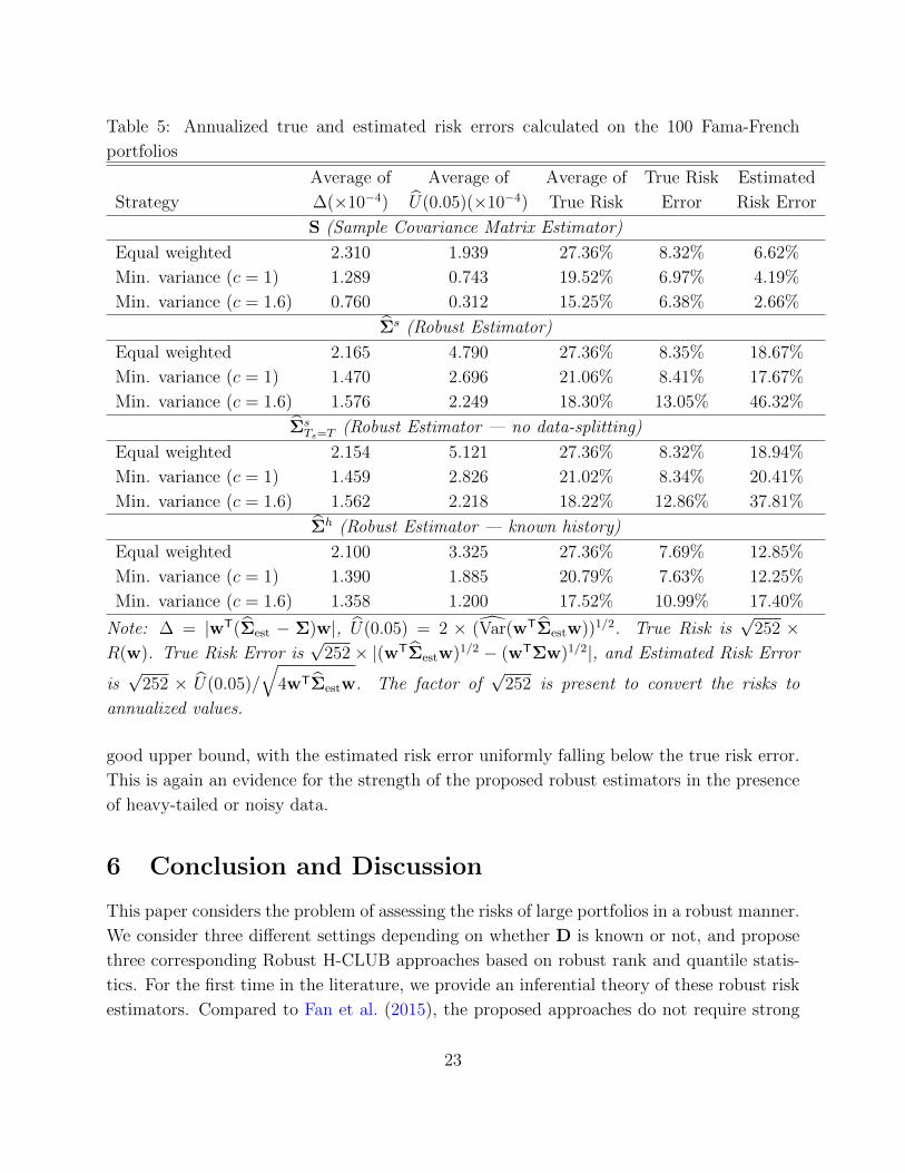
√252× |(wTΣestw)1/2 − (wTΣw)1/2|, and Estimated Risk Error

is√

252 × U(0.05)/

√4wTΣestw. The factor of

√252 is present to convert the risks to

annualized values.

good upper bound, with the estimated risk error uniformly falling below the true risk error.

This is again an evidence for the strength of the proposed robust estimators in the presence

of heavy-tailed or noisy data.

6 Conclusion and Discussion

This paper considers the problem of assessing the risks of large portfolios in a robust manner.

We consider three different settings depending on whether D is known or not, and propose

three corresponding Robust H-CLUB approaches based on robust rank and quantile statis-

tics. For the first time in the literature, we provide an inferential theory of these robust risk

estimators. Compared to Fan et al. (2015), the proposed approaches do not require strong

23

moment assumptions on the data. Both theoretical and empirical results verify that the

Robust H-CLUB approaches are more appropriate for studying heavy-tailed asset returns.

In the present paper, we do not impose any structural assumption on the covariance

matrix, such as the low rank plus sparse structure induced by the factor model. Fan et al.

(2015) propose methods based on factor-based covariance matrix estimators proposed in Fan

et al. (2008) and Fan et al. (2013). A natural extension to Fan et al. (2013) is to use Σ

(or Σh, Σs), instead of the sample covariance S, as the pilot estimator and plug it into the

POET algorithm (Fan et al., 2013). This constructs another robust risk estimator. We plan

to investigate the theoretical properties of such robust risk estimators and their limiting

distributions in the future.

The results in this paper also raise a number of interesting questions for future research.

One example is on deriving the limiting distributions of functionals of Σ other than wTΣw.

For example, Han and Liu (2014a) study the limiting distribution of ‖Σ‖max as T, d→∞ in

the setting that the observations are mutually independent. It is interesting to investigate

such asymptotic theory for a multivariate time series.

7 Proofs

In this section we provide the proofs of results in Section 3. In the sequel, using Assumption

(A1), we assume that ‖w‖ = 1 and ‖Σ‖max ≤ 1 without loss of generality.

7.1 Supporting Lemmas

Lemma 7.1 (Kontorovich et al. (2008) and Mohri and Rostamizadeh (2010)). Let f : ΩT →R be a measurable function that is c-Lipschitz with regard to the Hamming metric for some

c > 0:

supx1,...,xt,x′t

∣∣∣f(x1, . . . , xt, . . . , xT )− f(x1, . . . , x′t, . . . , xT )

∣∣∣ ≤ c,

and X1, . . . , XT be a sequence of stationary φ-mixing random variables. Then, for any ε > 0,

the following inequality holds:

P|f(X1, . . . , XT )− Ef(X1, . . . , XT )| ≥ ε

≤ 2 exp

[− 2ε2

Tc21 + 2∑T

k=1 φ(k)

].

Lemma 7.2 (Yoshihara (1976)). Let Xtt∈Z be a stationary process with the distribution

function F . For T ≥ m, we define

UT (g) =

(T

m

)−1 ∑

i1<···<img(Xi1 , . . . ,Xim)

24

be a U -statistic with order m and kernel function g. Let the function gi(·) be defined as

gi(X1, . . . ,Xi) =

∫g(X1, . . . ,Xm)dF (Xi+1) . . . dF (Xm),

for 1 ≤ i ≤ m, and let parameters θ and σ2 be defined as

θ =

∫g(X1, . . . ,Xm)dF (X1) . . . dF (Xm),

σ2 = 4(Eg1(X1)

2 − θ2 + 2∞∑

h=1

(Eg1(X1)g1(X1+h)− θ2

)). (7.1)

Suppose there exists a constant δ > 0 such that for r = 2 + δ, the following conditions hold:

1.

∫ ∣∣g(X1, . . . ,Xm)∣∣rdF (X1) . . . dF (Xm) ≤M0 <∞ for some constant M0;

2. E∣∣g(X1, . . . ,Xm)

∣∣r ≤M1 for some constant M1;

3. Xtt∈Z is β-mixing with β(n) = On−(2+δ′)/δ′ for some 0 < δ′ < δ.

Assuming that the above conditions hold, we then have

√TUT (g)− θ

σ

d→ Z, as T →∞,

where Z ∼ N(0, 1) is a standard Gaussian random variable.

Lemma 7.3 (Yoshihara (1976)). Let Xtt∈Z be a d-dimensional stationary process with the

marginal distribution function F , and X1, . . . ,XT be a sequence of observations. Suppose

h(·) : Rd × Rd → R is a kernel function such that for some constants ζ > 0 and H > 0, we

have∫ ∫

|h(X1,X2)|2+ζdF (X1)dF (X2) ≤ H, (7.2)∫|h(X1,X1+k)|2+ζdP(X1,X1+k) ≤ H, for all k ≥ 0, k ∈ Z, (7.3)

where P(Xt1 ,Xt2) is the joint distribution function of (Xt1 ,Xt2). For arbitrary random

vectors X,Y , we define

h1(X) =

∫h(X,Y )dF (Y )−

∫ ∫h(X,Y )dF (X)dF (Y ),

h2(X,Y ) = h(X,y)− h1(X)− h1(Y )−∫ ∫

h(X,Y )dF (X)dF (Y ).

25

If the process Xtt∈Z is β-mixing with mixing coefficient β(n) = On−(2+ζ′)/ζ′ for a con-

stant ζ ′ ∈ (0, ζ), then, for the U -statistic

UT (h2) :=2

T (T − 1)

∑

t1<t2

h2(Xt1 ,Xt2),

we have

ETUT (h2)2 ≤ 4

T (T − 1)2

∑

1≤t1<t2≤T

∑

1≤t3<t4≤T

∣∣∣Eh2(Xt1 ,Xt2)h2(Xt3 ,Xt4)∣∣∣

≤ 4

n3

T∑

t1,t2,t3,t4=1

∣∣∣Eh2(Xt1 ,Xt2)h2(Xt3 ,Xt4)∣∣∣ = O(T−λ),

where λ := min(2(ζ − ζ ′)/ζ ′(2 + ζ), 1

).

Lemma 7.4. Let Xtt∈Z be a d-dimensional stationary process with the marginal distri-

bution function F , X1, . . . ,XT be a sequence of observations, and X∗1 , . . . ,X∗T be a block

bootstrapped sample with block length l T 1−ε0 defined in Section 2.1. For a kernel function

h : Rd × Rd → R, define

UT (h) =2

T (T − 1)

∑

t1<t2

h(Xt1 ,Xt2) and U∗T (h) =2

T (T − 1)

∑

t1<t2

h(X∗t1 ,X∗t2

)

to be the U -statistics based on the observed sample and bootstrap sample, respectively. Now

supposing that h satisfies (7.2) and (7.3), and the process Xtt∈Z is β-mixing with mixing

coefficient β(n) = On−(2+ζ′)/ζ′ for a constant ζ ′ ∈ (0, ζ), we have∣∣∣Var∗

√TU∗T (h)

− Var

√TUT (h)

∣∣∣ = oP (1),

where Var∗ is the variance operator of the resampling distribution P∗ conditional onX1, . . . ,XT .

Proof. We define ω :=

∫ ∫h(X,Y )dF (X)dF (Y ). Using Hoeffding’s decomposition, we

have

U∗T (h) = ω +2

T

T∑

t=1

h1(X∗t ) + U∗T (h2).

The fact that for two random variables X and Y , we have Var(X+Y ) = Var(X)+Var(Y )+

2 Cov(X, Y ) ≤ Var(X) + Var(Y ) + 2√

Var(X)√

Var(Y ), yields

Var∗√TU∗T (h) ≤Var∗

2√T

T∑

t=1

h1(X∗t )

+ Var∗√

TU∗T (h2)

+ 2

√√√√Var∗ 2√

T

T∑

t=1

h1(X∗t )√

Var∗√

TU∗T (h2). (7.4)

26

Similarly, using the fact that Var(X + Y ) = Var(X) + Var(Y ) + 2 Cov(X, Y ) ≥ Var(X) +

Var(Y )− 2√

Var(X)√

Var(Y ), we have

Var∗√TU∗T (h) ≥Var∗

2√T

T∑

t=1

h1(X∗t )

+ Var∗√

TU∗T (h2)

− 2

√√√√Var∗ 2√

T

T∑

t=1

h1(X∗t )√

Var∗√

TU∗T (h2). (7.5)

By Theorem 2.3 of Shao and Yu (1993), regarding h1, we have

∣∣∣Var∗ 2√

T

T∑

t=1

h1(X∗t )− Var

2√T

T∑

t=1

h1(Xt)∣∣∣ a.s.−→ 0 (7.6)

On the other hand, by Lemma 7.3, we have Var√TUT (h2) = o(1) and Var∗

√TU∗T (h2) =

oP (1). Combining them with (7.4) and (7.5), we have

Var∗√TU∗T (h) = Var∗

2√T

T∑

t=1

h1(X∗t )

+ oP (1). (7.7)

Similar arguments yield that

Var√TUT (h) = Var

2√T

T∑

t=1

h1(Xt)

+ o(1). (7.8)

Combining (7.7) and (7.8), we obtain

Var∗√TU∗T (h) − Var

√TUT (h)=Var∗

2√T

T∑

t=1

h1(X∗t )−Var

2√T

T∑

t=1

h1(Xt)

+oP (1).

Combining the above equation with (7.6) completes the proof.

Lemma 7.5. Let Xtt∈Z be a stationary sequence of φ-mixing random vectors. Suppose

the φ-mixing coefficient satisfies Assumption (A3). Then we have

‖ET−T‖max = O(

1/T),

where T and T are sample and population Kendall’s tau matrix defined in (2.1).

Proof. For any two constant 1 ≤ s < t ≤ T , we have

P(Xtj −Xsj > 0, Xtk −Xtk > 0) = P(Xtj > Xsj, Xtk > Xsk).

27

Let

−∞ = a0 < −M < a1 < . . . < ah−1 < M < ah =∞and

−∞ = b0 < −M < b1 < . . . < bh−1 < M < bh =∞be two pre-determined real sequences. Note that for i0 = 1, . . . , h, given Xsj ∈ [ai0−1, ai0 ],the event Xtj > Xsj implies the event Xtj > ai0−1. This yields

P(Xtj > Xsj, Xtk > Xsk) ≤∑

i0,j0

P(Xtj > ai0−1, Xtk > bj0−1 |Xsj ∈ [ai0−1, ai0 ], Xsk ∈ [bj0−1, bj0 ])·

P(Xsj ∈ [ai0−1, ai0 ], Xsk ∈ [bj0−1, bj0 ]).

On the other hand, given Xsj ∈ [ai0−1, ai0 ], the event Xtj > ai0 implies the event

Xtj > Xsj. Thus, we have

P(Xtj > Xsj, Xtk > Xsk) ≥∑

i0,j0

P(Xtj > ai0 , Xtk > bj0 |Xsj ∈ [ai0−1, ai0 ], Xsk ∈ [bj0−1, bj0 ])·

P(Xsj ∈ [ai0−1, ai0 ], Xsk ∈ [bj0−1, bj0 ]).

Now, we define ψUh to be

ψUh :=∑

i0,j0

P(Xtj > ai0−1, Xtk > bi0−1)P(Xsj ∈ [ai0−1, ai0 ], Xsk ∈ [bj0−1, bj0 ]),

and similarly define ψLh to be

ψLh =∑

i0,j0

P(Xtj > ai0 , Xtk > bi0)P(Xsj ∈ [ai0−1, ai0 ], Xsk ∈ [bj0−1, bj0 ]).

Let ψh be either ψUh or ψLh with regard to the sign of P(Xtj > Xsj, Xtk > Xsk)− ψLh :

ψh =

ψLh , if P(Xtj > Xsj, Xtk > Xsk) > ψLh ;

ψUh , Otherwise..

Without loss of generality, supposing that we have P(Xtj > Xsj, Xtk > Xsk) > ψLh , it follows

that∣∣∣P(Xtj > Xsj, Xtk > Xsk)− ψh

∣∣∣ = P(Xtj > Xsj, Xtk > Xsk)− ψLh≤∑

i0,j0

∣∣∣P(Xtj>aj0−1, Xtk>bj0−1 |Xsj∈ [ai0−1, ai0 ], Xsk∈ [bj0−1, bj0 ])−P(Xtj > aj0 , Xtk > bj0)∣∣∣·

P(Xsj ∈ [ai0−1, ai0 ], Xsk ∈ [bj0−1, bj0 ])

≤φ(t− s) + maxi0,j0|P(Xtj > aj0−1, Xtk > bj0−1)− P(Xtj > aj0 , Xtk > bj0)|.

28

Now let h → ∞, maxh−1i=2 |ai − ai−1| → 0, maxh−1i=2 |bi − bi−1| → 0, and M → ∞. By the

definition of φ-mixing coefficient, we have

∣∣∣P(Xtj > Xsj, Xtk > Xsk)−∫

P(Xtj > a,Xtk > b)dP(Xsj = a,Xsk = b)∣∣∣ ≤ φ(s− t). (7.9)

Moreover, letting X ′ = (X ′1, . . . , X′d)T have the same distribution as X1 and independent of

(Xs,Xt), we have

dP(Xsj = a,Xsk = b) = dP(X ′j = a,X ′k = b).

This yields

∫P(Xtj > a,Xtk > b)dP(Xsj = a,Xsk = b) =

∫P(Xtj > a,Xtk > b)dP(X ′j = a,X ′k = b).

Plugging the above equation into (7.9), we obtain

∣∣∣P(Xtj > Xsj, Xtk > Xsk)−∫

P(Xtj > a,Xtk > b)dP(X ′j = a,X ′k = b)∣∣∣ ≤ φ(t− s).

Note that by the definition of conditional probability, we have

∫P(Xtj > a,Xtk > b)dP(X ′j = a,X ′k = b) = P(Xtj −X ′j > 0, Xtk −X ′k > 0).

Thus, combining the above two equations, we have∣∣∣P(Xtj −Xsj > 0, Xtk −Xsk > 0)− P(Xtj −X ′j > 0, Xtk −X ′k > 0)

∣∣∣ ≤ φ(t− s). (7.10)

Using similar arguments, we can prove∣∣∣P(Xtj −Xsj < 0, Xtk −Xsk < 0)− P(Xtj −X ′j < 0, Xtk −X ′k < 0)

∣∣∣ ≤ φ(t− s), (7.11)∣∣∣P(Xtj −Xsj < 0, Xtk −Xsk > 0)− P(Xtj −X ′j < 0, Xtk −X ′k > 0)

∣∣∣ ≤ φ(t− s), (7.12)∣∣∣P(Xtj −Xsj > 0, Xtk −Xsk < 0)− P(Xtj −X ′j > 0, Xtk −X ′k < 0)

∣∣∣ ≤ φ(t− s). (7.13)

By definition, we have τjk = Esign(Xtj − X ′j)(Xtk − X ′k). Applying the definition of

expectation, we have

τjk =P(Xtj −X ′j > 0, Xtk −X ′k > 0) + P(Xtj −X ′j < 0, Xtk −X ′k < 0)−P(Xtj −X ′j > 0, Xtk −X ′k < 0)− P(Xtj −X ′j < 0, Xtk −X ′k > 0). (7.14)

29

By the same reason, we have

Esign(Xtj −Xsj)(Xtk −Xsk)=P(Xtj −Xsj > 0, Xtk −X ′sk > 0) + P(Xtj −Xsj < 0, Xtk −Xsk < 0)−

P(Xtj −Xsj > 0, Xtk −Xsk < 0)− P(Xtj −Xsj < 0, Xtk −Xsk > 0). (7.15)

Now, by the definition of τjk, we have∣∣∣Eτjk − τjk

∣∣∣ =∣∣∣E 2

T (T − 1)

∑

s<t

sign(Xtj −Xsj)(Xtk −Xsk)− τjk

∣∣∣

≤ 2

T (T − 1)

∑

s<t

∣∣∣Esign(Xtj −Xsj)(Xtk −Xsk)− τjk∣∣∣.

Plugging (7.14) and (7.15) into the above equation, and applying (7.10) - (7.13), we obtain

∣∣∣Eτjk − τjk∣∣∣ ≤ 2

T (T − 1)

∑

s<t

4φ(t− s) =8∑T

t=1(T − t)φ(t)

T (T − 1)= O

( 1

T

). (7.16)

The last inequality is because by Assumption (A3), we have

T∑

t=1

(T − t)φ(t) ≤T∑

t=1

T − tt1+ε

≤ T

∞∑

t=1

1

t1+ε= O(T ).

This completes the proof.

Lemma 7.6. Let Xtt∈Z be a stationary sequence of φ-mixing random vectors. Suppose

the φ-mixing coefficient satisfies Assumption (A3). Then we have

‖T−T‖max = OP

(√ log d

T

),

where T and T are the sample and population Kendall’s tau matrix based on XtTt=1.

Proof. Consider the following function

fjk(X1, . . . ,XT ) :=2

T − 1

∑

t<t′

sign(Xtj −Xt′j)sign(Xtk −Xt′k) = T · τjk.

We have∣∣∣fjk(X1, . . . ,Xi, . . . ,XT )− fjk(X1, . . . ,X

′i, . . . ,XT )

∣∣∣

=2

T − 1

∣∣∣∑

t6=isign(Xij −Xtj)sign(Xik −Xtk)−

∑

t6=i′sign(Xi′j −Xtj)sign(Xi′k −Xtk)

∣∣∣

≤ 2

T − 12(T − 1) = 4.

30

Thus, fjk is c-Lipschitz with respect to the Hamming metric. By Lemma 7.1, we have

P(T |τjk − Eτjk| ≥ ε

)≤ 2 exp

[− ε2

8T1 + 2∑∞

l=1 φ(l)],

for any ε > 0. Here∑∞

l=1 φ(l) <∞ is guaranteed by Assumption (A3). Thus, we have

P(‖T− ET‖max ≥ ε

)≤

d∑

j,k=1

P(|τjk − Eτjk| ≥ ε

)≤ 2 exp

[2 log d− Tε2

81 + 2∑∞

l=1 φ(l)].

Setting ε =√

[241 + 2∑∞

l=1 φ(l) log d]/T , we have

‖T− ET‖max = OP

(√ log d

T

).

Combining the above equation with Lemma 7.5 completes the proof.

Lemma 7.7. [Theorem 1 in Doukhan and Neumann (2007)] Suppose that X1, . . . , XT are

real-valued random variables with mean 0, defined on a common probability space (Ω,A,P).

Let Ψ : N2 → N be one of the following functions:

(a). Ψ(u, v) = 2v,

(b). Ψ(u, v) = u+ v,

(c). Ψ(u, v) = uv,

(d). Ψ(u, v) = α(u+ v) + (1− α)uv, for some α ∈ (0, 1).

We assume that there exist constants K,M,L1, L2 > 0, a, b ≥ 0, and a non-increasing

sequence of real coefficients ρ(n)n≥0 such that for any u-tuple (s1, . . . , su) and v-tuple

(t1, . . . , tv) with 1 ≤ s1 ≤ · · · ≤ su ≤ t1 ≤ · · · ≤ tv ≤ T , the following inequalities hold:∣∣∣∣∣Cov

(u∏

i=1

Xsi ,

v∏

j=1

Xtj

)∣∣∣∣∣ ≤ K2Mu+v(u+ v)!bΨ(u, v)ρ(t1 − su), (7.17)

where for the sequence ρ(n)n≥0, we require that

∞∑

s=0

(s+ 1)kρ(s) ≤ L1Lk2(k!)a, ∀k ≥ 0. (7.18)

We also assume that the following moment condition holds:

E|Xt|k ≤ (k!)bMk, for all t = 1, . . . , T. (7.19)

31

Let ST =∑T

t=1Xt. Then, for all x > 0, we have

P(ST ≥ x) ≤ exp

− x2

C1T + C2x(2a+2b+3)/(a+b+2)

, (7.20)

where C1 and C2 are constants depending on K,M,L1, L2, a, and b:

C1 = 2a+b+3K2M2L1(K2 ∨ 2), C2 = 2ML2(K

2 ∨ 2)1/(a+b+2). (7.21)

Lemma 7.8. Let Xtt∈Z be a d dimensional stationary φ-mixing process satisfying As-

sumptions (A6), (A7), and (A9). Let R = diag(σM,1, . . . , σM,d) be a diagonal matrix of

sample median absolute deviations based on XtTt=1, and R = diagσM(X11), . . . , σM(X1d)be its population counterpart. Then we have

‖R−R‖max = OP

(√ log d

T

).

Proof. We first focus on a marginal process XtjTt=1. For notational brevity, we suppress

the index j and denote the process as XtTt=1. Define X = X1. Let F be the distribution

function of X and FT be the empirical distribution of XtTt=1 and F−1T (q) := Q(Xt; q) for

any q ∈ [0, 1]. By the definition of Q(·) in (2.3), we have, for any ε ∈ [0, 1],

ε ≤ FTF−1T (ε) ≤ ε+1

T.

This implies that

PQ(Xt; q)−Q(X; q) ≥ u

= P

F−1T (q)− F−1(q) ≥ u

≤ P

[q +

1

T≥ FTu+ F−1(q)

].

By the definition of FT , we further have


≤ P

[ T∑

t=1

IXt ≤ F−1(q) + u ≤ Tq + 1]

=P( T∑

t=1

[− IXt ≤ F−1(q) + u+ FF−1(q) + u

]≥ T

[FF−1(q) + u − q − 1

T

]).

Since Xtt∈Z is φ-mixing, the process −IXt ≤ F−1(q)+u+FF−1(q)+ut∈Z is also φ-

mixing. By Lemma 6 in Doukhan and Louhichi (1999), −IXt ≤ F−1(q)+u+FF−1(q)+

ut∈Z satisfies (7.17) with K = 2, M = 1, b = 0, any of the four Ψ functions, and

ρ(n) = φ(n) ≤ C1 exp(−C2nr).

32

By Proposition 8 in Doukhan and Neumann (2007), (7.18) is satisfied with a = max(1, 1/r)

and some constants L1 and L2. Since −IXt ≤ F−1(q) + u + FF−1(q) + u is bounded,

(7.19) is also satisfied with b = 0. Thus, applying Lemma 7.7, we have


≤ exp

(−ψ(FF−1(q) + u − q − 1

T

)), (7.22)

for FF−1(q) + u − q − 1/T > 0, where

ψ(x) :=Tx2

C1 + C2T (a+1)/(a+2)x(2a+3)/(a+2),

for x > 0, a = max(1, 1/r), and some absolute constants C1 and C2. On the other hand, we

have

PQ(Xt; q)−Q(X; q) ≤ −u

= P

F−1T (q)− F−1(q) ≤ −u

≤ P

[q ≤ FTF−1(q)− u

]

=P( T∑

t=1

[IXt ≤ F−1(q)− u − FF−1(q)− u

]≥ T

[q − FF−1(q)− u

]).

By similar arguments, we have

PQ(Xt; q)−Q(X; q) ≤ −u

≤ exp

(−ψ(q − FF−1(q)− u

)). (7.23)

Combining (7.22) and (7.23), we have

P∣∣∣Q(Xt; q)−Q(X; q)

∣∣∣ ≥ u

≤ exp(−ψ(FF−1(q) + u − q − 1

T

))+ exp

(−ψ(q − FF−1(q)− u

)), (7.24)

for FF−1(q) + u − q − 1/T > 0.

Next, we continue to derive exponential tail probabilities for σM(XtTt=1). We write

m := Q(XtTt=1; 1/2) and m := Q(X1; 1/2) to be the sample and population medians. Let

F1 and F2 be the distribution functions of X and |X −Q(X; 1/2)|. By the definition of σM,

we have

PσM

(XtTt=1

)− σM(X) > u

= P

Q(|Xt − m|

Tt=1

;1

2

)−Q

(|X −m|; 1

2

)> u

≤PQ(|Xt −m|

Tt=1

;1

2

)+ |m−m| −Q

(|X −m|; 1

2

)> u

≤PQ(|Xt −m|

Tt=1

;1

2

)−Q

(|X −m|; 1

2

)>u

2

+ P

(|m−m| > u

2

). (7.25)

33

On the other hand, using the same technique, we have

PσM

(XtTt=1

)− σM(X) < −u

= P

Q(|Xt − m|

Tt=1

;1

2

)−Q

(|X −m|; 1

2

)< −u

≤PQ(|Xt −m|

Tt=1

;1

2

)− |m−m| −Q

(|X −m|; 1

2

)< −u

≤PQ(|Xt −m|

Tt=1

;1

2

)−Q

(|X −m|; 1

2

)< −u

2

+ P

(|m−m| > u

2

). (7.26)

Combining (7.25) and (7.26), we have

P|σM(XtTt=1

)− σM(X)| > u

≤P∣∣∣Q

(|Xt −m|

Tt=1

;1

2

)−Q

(|X −m|; 1

2

)∣∣∣ > u

2

+ 2P

(|m−m| > u

2

). (7.27)

Now applying Inequality (7.24), we have

P|Q(|Xt −m|

Tt=1

;1

2

)−Q

(|X −m|; 1

2

)| > u

2

≤ exp(−ψ[F2

F−12

(1

2

)+u

2

− 1

2− 1

T

])+ exp

(−ψ[1

2− F2

F−12

(1

2

)− u

2

])

≤ exp−ψ(ηu

2− 1

T

)+ exp

−ψ(ηu

2

), (7.28)

whenever F2F−12 (1/2) + u/2 − 1/2 > 1/T . Here the last inequality is due to Assumption

(A9) and the fact that ψ is non-decreasing. Similarly, we also have

P(|m−m| > u

2

)

≤ exp(−ψ[F1

F−11

(1

2

)+u

2

]− 1

2− 1

T

)+ exp

(−ψ[1

2− F1

F−11

(1

2

)− u

2

])

≤ exp−ψ(ηu

2− 1

T

)+ exp

−ψ(ηu

2

), (7.29)

whenever F1F−11 (1/2) + u/2− 1/2 > 1/T . Again the last inequality is due to Assumption

(A9) and the fact that f is nondecreasing. Here we recall that F1 and F2 are the distribution

functions of X and |X − Q(X; 1/2)|. Combining Inequalities (7.27), (7.28), and (7.29), we

have

P∣∣∣σM

(XtTt=1

)− σM(X)

∣∣∣ > u≤3 exp

−ψ(ηu

2− 1

T

)+ 3 exp

−ψ(ηu

2

)

≤6 exp−ψ(ηu

2− 1

T

),

34

whenever we have 0 < u/2 < κ and ηu/2 > 1/T . Now we switch the focus back to the entire

matrix R. By the sub-additivity of probability measures, we have

P(‖R−R‖max > u

)≤

d∑

j=1

P∣∣∣σM

(XtjTt=1

)− σM(X1j)

∣∣∣ > u

≤6 exp

2 log d− ψ(ηu

2− 1

T

). (7.30)

We recall that by the definition of the function ψ(·), we have

ψ(ηu

2− 1

T

)=

T(ηu2− 1

T

)2

C1 + C2T (a+1)/(a+2)(ηu2− 1

T

)(2a+3)/(a+2).

To simplify the denominator on the right-hand side of the above equation, we require that

C1 ≥ C2T(a+1)/(a+2)

(ηu2− 1

T

)(2a+3)/(a+2)

. (7.31)

Then we have ψ(ηu/2− 1/T ) ≥ T/(2C1)(ηu/2− 1/T )2. Plugging this into (7.30), we obtain

P(‖R−R‖max > u

)≤ 6 exp

2 log d− T

2C1

(ηu2− 1

T

)2. (7.32)

Next we select a proper u to derive the rate of convergence. To this end, we set

2 log d− T

2C1

(ηu2− 1

T

)2= − log d.

This leads to

u =2

η

(√6C1 log d

T+

1

T

). (7.33)

Plugging the above equation into (7.31), we get

C1 ≥ 6(2a+3)/(2a+4)C2

(log d)2a+3

T

1/(2a+4)

.

Thus, (7.31) holds as long as we have log d = o[T 1/(2a+3)]. By Assumption (A7), (7.31)

holds. Plugging (7.33) into (7.32), we get

P‖R−R‖max >

2

η

(√6C1 log d

T+

1

T

)≤ 6

d.

Thus, as T and d both go to infinity, we have

‖R−R‖max = OP

(√ log d

T

).

This completes the proof.

35

Lemma 7.9. Let XtTt=1 be a d dimensional stationary process satisfying Assumptions

(A6) - (A9). We then have

‖D−D‖max = OP

(√ log d

T

),

where D is defined in Equation (2.13).

Proof. Define R = diag(σM,1, . . . , σM,d), R = diagσM(X11), . . . , σM(X1d), cM = σ1/σM,1,

and cM =√

Σ11/σM(X11). We have

‖D−D‖max = ‖cMR− cMR‖max ≤ ‖cM(R−R)‖max + ‖(cM − cM)R‖max

≤ |cM|‖R−R‖max + C|cM − cM|. (7.34)

By Lemma 7.8, we have

‖R−R‖max = OP

(√ log d

T

). (7.35)

Thus, specifically, we have

σM,1P→ σM(X11). (7.36)

We can rewrite σ21 as

σ21 =

1

T − 1

T∑

t=1

(Xt1 − XT1)2 =

2

T (T − 1)

∑

t<t′

h(Xt1, Xt′1),

where XT1 :=∑T

t=1Xtj/T , and h(Xt1, Xt′1) = (Xt1 − Xt′1)2/2. Thus, σ2

1 is a U -statistic

with kernel function h. Using Lemma 7.2 with Assumptions (A6) and (A8), we have√T (σ2

1 −Σ11)d→ Z1 where Z1 is a Gaussian random variable with mean 0. Using the delta

method, we have√T (σ1 −

√Σ11)

d→ Z2 for another mean 0 Gaussian random variable Z2.

Combining this with (7.36) and applying Slutsky’s theorem, we have√T (cM− cM)

d→ Z3 for

some Gaussian random variable Z3. Thus, we have

|cM − cM| = OP

(1/√T). (7.37)

Combining (7.34), (7.35), and (7.37), we have the desired result.

36

7.2 Proof of Theorem 3.1

Proof. Denote a = Dw. Using Taylor expansion entry-wise on sin(πT/2) at sin(πT/2), we

have

wT(Σ−Σ)w = aT

sin(π

2T)− sin(

π

2T)a

=aT

cos(π

2T) π

2(T−T)

a

︸︷︷︸A1

+aT−1

2[sin(θjk)] (

π

2)2(T−T) (T−T)

a

︸︷︷︸A2

,

where for each j, k ∈ 1, . . . , d, θjk lies between τjk and τjk. Using Lemma 7.6 and assump-

tion (A4), we have

A2 ≤π2

8‖a‖21‖T−T‖2max = OP

( log d

T

)= oP

( σ√T

). (7.38)

Here the first inequality is due to the fact that for any vectors v1,v2 ∈ Rd and matrix

M ∈ Rd×d,

|vT1 Mv2| ≤ ‖v1‖1‖Mv2‖∞ ≤ ‖M‖max‖v1‖1‖v2‖1. (7.39)

Next, we focus on A1. We can expand A1 by

A1 =2

T (T − 1)

∑

t<t′

g(Rt,Rt′)

︸︷︷︸UT

−aT

cos(π

2T) π

2Ta, (7.40)

where g(·) is defined in Equation (3.1). Note that UT is a U -statistic of order 2 and the

kernel function g(·) satisfying

∣∣∣g(Rt,Rt′)∣∣∣ ≤ π

2maxjk

∣∣∣sign(Rtj −Rt′j)sign(Rtk −Rt′k)∣∣∣‖a‖21 ≤

π

2‖D‖max‖w‖21 ≤

π

2.

Thus g(·) is a bounded kernel function. Assumption (A3) guarantees that Rtt∈Z is also

β-mixing with β(n) ≤ n−1−ε. Thus, by Lemma 7.2, we have

√TA1

σ=

√T (UT − θ)

σ

d→ Z, (7.41)

where Z ∼ N(0, 1) is a standard Gaussian random variable. By Slutsky’s theorem, combining

the above equation with (7.38) leads to the desired result.

37


Proof. Similar to the proof of Theorem 3.1, we can expand wT(Σ∗ −Σ)w by

wT(Σ∗−Σ)w=aTcos(

π

2T)π

2(T∗−T)

a

︸︷︷︸A∗1

+aT−1

2[sin(θjk)](

π

2)2(T∗−T)(T∗−T)

a

︸︷︷︸A∗2

. (7.42)

Let R∗ := wT(Σ∗ −Σ)w and rewrite A∗1 as

A∗1 =2

T (T − 1)

∑

t<t′

g(R∗t ,R∗t′)

︸︷︷︸U∗T

−aT

cos(π

2T) π

2Ta.

Remind that g(·) is a bounded kernel function and Assumption (A3) implies that the process

Rtt∈Z is β-mixing with β(n) ≤ n−1−ε. By Lemma 7.4 and Assumption (A2), we then have∣∣∣Var∗(

√TU∗T )− Var(

√TUT )

∣∣∣ = oP (σ2),

where UT is defined in Equation (7.40). Moreover, by (7.41), we have Var(√TUT ) = σ21 +

o(1). Thus, we have

Var∗(√TA∗1) = Var∗(

√TU∗T ) = σ21 + oP (1). (7.43)

Next, we focus on the asymptotics of Var∗(√TA∗2). Noting that by (7.39), we have

A∗2 ≤π2

4‖a‖21‖T∗ −T‖2max.

By the circular block bootstrap procedure, the process R∗tt∈Z is still a φ-mixing process

with mixing coefficient φ(n) ≤ n−(1+ε)(1−ε0) = O(n−1−ε2) for some ε2 > 0 as long as ε >

ε0/(1 − ε0). Thus, by Lemma 7.6, we have ‖T∗ − T‖max = OP (√

log d/T ). Thus, we have

A∗2 = OP (log d/T ) and accordingly

Var∗(√TA∗2) ≤ TE∗(A∗22 ) = OP

(log d)2

T

= oP (σ2), (7.44)

where E∗ is the bootstrap expectation conditional on RtTt=1. Combining Equations (7.42),

(7.43), and (7.44), we have

Var∗(√TR∗) = Var∗

√T (A∗1 + A∗2)

= Var∗(

√TA∗1) + Var∗(

√TA∗2) + 2 Cov(

√TA∗1,

√TA∗2)

≤ Var∗(√TA∗1) + Var∗(

√TA∗2) + 2

√Var∗(

√TA∗1)

√Var∗(

√TA∗2)

= σ21 + oP (1). (7.45)

38

On the other hand, we also have

Var∗(√TR∗) ≥ Var∗(

√TA∗1) + Var∗(

√TA∗2)− 2

√Var∗(

√TA∗1)

√Var∗(

√TA∗2)

= σ21 + oP (1). (7.46)

Combining (7.45) and (7.46) completes the proof.


Proof. Denote a := Dw. We can write

wT(Σs−Σ)w=aT

sin(π

2Ts)−sin(

π

2T)a

︸︷︷︸B1

+wTD sin(

π

2Ts)Dw−wTD sin(

π

2Ts)Dw

︸︷︷︸B2

. (7.47)

By the same arguments as in the proof of Theorem 3.1, we have

√TsB1

σ

d→ Z, (7.48)

where Z ∼ N(0, 1) is a Gaussian random variable. It remains to show that B2 is ignorable

asymptotically. Using (7.39), we have

|B2| ≤∣∣∣wTD sin(

π

2Ts)(D−D)w

∣∣∣+∣∣∣wT(D−D) sin(

π

2Ts)Dw

∣∣∣

≤ ‖ sinπ

2T‖max‖(D−D)w‖1(‖Dw‖1 + ‖Dw‖1)

≤ ‖D−D‖max(‖D‖max + ‖D‖max).

Using Lemma 7.9 and Assumption (A5), we have |B2| = OP (√

log d/T ) = oP (σ/√Ts).

Together with (7.47) and (7.48), using Slutsky’s theorem, we have the desired result.

7.5 Proof of Corollary 3.1

Proof. By (3.5), we have P(|wj/wj − 1| > t) ≤ exp(−CTt2). Thus, we further have

P(maxj|wj/wj − 1| > t) ≤ dP(|wj/wj − 1| > t) ≤ exp(log d− CTt2).

To simplify the rate of convergence, setting t =√

(3 log d)/(CT ), we have

P(

maxj|wj/wj − 1| >

√3 log d/(CT )

)≤ 1/d.

39

Thus, as (T, d) go to infinity, we have maxj |wj/wj − 1| = OP (√

log d/T ). This gives us an

upper bound of the convergence rate of ‖w −w‖1:

‖w−w‖1 =d∑

j=1

|wj−wj|=d∑

j=1

|wj| ·∣∣∣wjwj−1∣∣∣≤‖w‖1 ·max

j

∣∣∣wjwj−1∣∣∣ = OP

(√ log d

T

). (7.49)

Similar as in (7.47), we can decompose wTΣsw −wTΣw into

wTΣsw −wTΣw = B1 + wTD sin(π

2Ts)Dw −wTD sin(

π

2Ts)Dw

︸︷︷︸B3

, (7.50)

where B1 is defined in (7.47). As in the proof of Theorem 3.5, we still have (7.48). Regarding

B3, we have |B3| ≤ ‖Dw −Dw‖1‖Dw + Dw‖1. Using the triangle inequality, we have

|B3| ≤(‖D(w −w)‖1 + ‖(D−D)w‖1

)(‖D‖1‖w‖1 + ‖D‖1‖w‖1

)

≤(‖D‖max‖w −w‖1 + ‖D−D‖max

)(‖D‖max‖w‖1 + ‖D‖max

).

Using (7.49) and Lemma 7.9, we can conclude |B3| = OP (√

log d/T ). Plugging it into (7.50)

and using the Slutsky’s theorem, we have the desired result.


Proof. Let Ks∗ = sin(πTs∗/2) and K = sin(πT/2). We can decompose R∗s := wTDKs∗Dw

into two parts:

R∗s = wTDKs∗Dw −wTDKDw︸︷︷︸B∗1

+ wTDKs∗Dw −wTDKs∗Dw︸︷︷︸B∗2

. (7.51)

By similar arguments as in the proof of Theorem 3.2, we have

Var∗(√TsB

∗1) = σ21 + oP (1). (7.52)

Next, we show that Var∗(√TsB

∗2) = oP (σ2). We can upper bound Var∗(B∗2) by

Var∗(B∗2) = Var∗

wTDKs∗(D−D)w + wT(D−D)Ks∗Dw

≤Var∗

wTDKs∗(D−D)w

+ Var∗

wT(D−D)Ks∗Dw

+ 2

√Var∗

wTDKs∗(D−D)w

√Var∗

wT(D−D)Ks∗Dw

. (7.53)

40

For any random matrix X := (R1, . . . ,Rm)T ∈ Rm×n and fixed vectors v1 ∈ Rm, v2 ∈ Rn,

let V be a matrix with (j, k) entry vT2 Cov(Rj,Rk)v2. It is easy to verify that

Var(vT1 Xv2) =vT

1 Var(Xv2)v1 = vT1 Vv1 ≤ ‖v1‖21 max

jk

∣∣∣vT2 Cov(Rj,Rk)v2

∣∣∣

≤‖v1‖21‖v2‖21 maxj1,k1,j2,k2

|Cov(Rj1,k1,Rj2,k2)|. (7.54)

Now writing v1 = Dw, v2 = (D−D)w, and X = Ks∗ , we have

Var∗

wTDKs∗(D−D)w≤‖Dw‖21‖(D−D)w‖21 max

j1,k1,j2,k2|∗

Cov(τ s∗j1,k1

, τ s∗j2,k2

)|

≤‖w‖41‖D‖2max‖D−D‖2max = ‖D‖2max‖D−D‖2max. (7.55)

Note that D only depends on RtTt=1 and is thus fixed under Var∗(·). Using Lemma 7.9

and (7.55), we have

Var∗√

TswTDKs∗(D−D)w

= OP

(Ts

log d

T

)= OP

( log d

T δ

)= oP (σ2). (7.56)

Similarly, we also have

Var∗√

TswT(D−D)Ks∗Dw

= oP (σ2). (7.57)

Combining (7.53), (7.56), and (7.57), we have

Var∗(√TsB

∗2) = oP (σ2). (7.58)

By (7.51), we have

Var∗(√TsR

∗) ≥ Var∗(√TsB

∗1) + Var∗(

√TsB

∗2)− 2

√Var∗(

√TsB∗1)

√Var∗(

√TsB∗2),

and similarly

Var∗(√TsR

∗) ≤ Var∗(√TsB

∗1) + Var∗(

√TsB

∗2) + 2

√Var∗(

√TsB∗1)

√Var∗(

√TsB∗2).

Using the above two inequalities with (7.52) and (7.58), we can conclude that Var∗(√TsR

∗) =

σ21 + oP (1).

7.7 Proofs of Theorems 3.3 and 3.4

The proofs of Theorems 3.3 and 3.4 are close to those of Theorems 3.5 and 3.6. The main

difference is that now Th plays the role of T , and T plays the role of Ts. We accordingly

omit the proofs.

41

References

Agarwal, A., Negahban, S., and Wainwright, M. J. (2012). Noisy matrix decomposition via

convex relaxation: Optimal rates in high dimensions. The Annals of Statistics, 40(2):1171–

1197.

Bai, J. and Liao, Y. (2012). Efficient estimation of approximate factor models via regularized

maximum likelihood. arXiv preprint arXiv:1209.5911.

Barndorff-Nielsen, O. E. (2002). Econometric analysis of realized volatility and its use in

estimating stochastic volatility models. Journal of the Royal Statistical Society: Series B

(Statistical Methodology), 64(2):253–280.

Bickel, P. J. and Levina, E. (2008a). Covariance regularization by thresholding. The Annals

of Statistics, 36(6):2577–2604.

Bickel, P. J. and Levina, E. (2008b). Regularized estimation of large covariance matrices.

The Annals of Statistics, 36(1):199–227.

Bollerslev, T. (1986). Generalized autoregressive conditional heteroskedasticity. Journal of

Econometrics, 31(3):307–327.

Cai, T. T., Zhang, C.-H., and Zhou, H. H. (2010). Optimal rates of convergence for covariance

matrix estimation. The Annals of Statistics, 38(4):2118–2144.

Cai, T. T. and Zhou, H. H. (2012). Optimal rates of convergence for sparse covariance matrix

estimation. The Annals of Statistics, 40(5):2389–2420.

Chamberlain, G. (1983). A characterization of the distributions that imply mean–variance

utility functions. Journal of Economic Theory, 29(1):185–201.

Chang, C. and Tsay, R. S. (2010). Estimation of covariance matrix via the sparse Cholesky

factor with lasso. Journal of Statistical Planning and Inference, 140(12):3858–3873.

Chen, X., Xu, M., and Wu, W. (2013). Covariance and precision matrix estimation for

high-dimensional time series. The Annals of Statistics, 41(6):2994–3021.

Cont, R. (2001). Empirical properties of asset returns: stylized facts and statistical issues.

Quantatitive Finance, 1(2):223–236.

Doukhan, P. and Louhichi, S. (1999). A new weak dependence condition and applications

to moment inequalities. Stochastic Processes and their Applications, 84(2):313–342.

42

Doukhan, P. and Neumann, M. H. (2007). Probability and moment inequalities for sums

of weakly dependent random variables, with applications. Stochastic Processes and their

Applications, 117(7):878–903.

Fan, J., Fan, Y., and Lv, J. (2008). High dimensional covariance matrix estimation using a

factor model. Journal of Econometrics, 147(1):186–197.

Fan, J., Han, F., and Liu, H. (2014). PAGE: Robust pattern guided estimation of large

covariance matrix. Technical report, Princeton University.

Fan, J., Liao, Y., and Mincheva, M. (2011). High dimensional covariance matrix estimation

in approximate factor models. The Annals of Statistics, 39(6):3320–3356.

Fan, J., Liao, Y., and Mincheva, M. (2013). Large covariance estimation by thresholding

principal orthogonal complements. Journal of the Royal Statistical Society: Series B

(Statistical Methodology), 75(4):603–680.

Fan, J., Liao, Y., and Shi, X. (2015). Risks of large portfolios. Journal of Econometrics (to

appear).

Fan, J. and Peng, H. (2004). Nonconcave penalized likelihood with a diverging number of

parameters. The Annals of Statistics, 32(3):928–961.

Fan, J., Zhang, J., and Yu, K. (2012). Vast portfolio selection with gross-exposure con-

straints. Journal of the American Statistical Association, 107(498):592–606.

Frahm, G. and Jaekel, U. (2007). Tyler’s M-estimator, random matrix theory, and generalized

elliptical distributions with applications to finance. Technical report, Helmut Schmidt

University.

Fryzlewicz, P. (2013). High-dimensional volatility matrix estimation via wavelets and thresh-

olding. Biometrika, 100(4):921–938.

Gomez, K. and Gallon, S. (2011). Comparison among high dimensional covariance matrix

estimation methods. Revista Colombiana de Estadıstica, 34(3):567–588.

Greenshtein, E. and Ritov, Y. (2004). Persistence in high-dimensional linear predictor selec-

tion and the virtue of overparametrization. Bernoulli, 10(6):971–988.

Hamada, M. and Valdez, E. (2004). CAPM and option pricing with elliptical distributions.

School of Finance and Economics, University of Technology, Sydney.

43

Han, F. and Liu, H. (2013a). Optimal rates of convergence for latent generalized correlation

matrix estimation in transelliptical distribution. arXiv preprint arXiv:1305.6916.

Han, F. and Liu, H. (2013b). Principal component analysis on non-Gaussian dependent data.

In Proceedings of the 30th International Conference on Machine Learning, pages 240–248.

Han, F. and Liu, H. (2013c). Transition matrix estimation in high dimensional time series.

In Proceedings of the 30th International Conference on Machine Learning, pages 172–180.

Han, F. and Liu, H. (2014a). Distribution-free tests of independence with applications to

testing more structures. arXiv preprint arXiv:1410.4179.

Han, F. and Liu, H. (2014b). Scale-invariant sparse PCA on high-dimensional meta-elliptical

data. Journal of the American Statistical Association, 109(505):275–287.

Han, F., Lu, J., and Liu, H. (2014). Robust scatter matrix estimation for high dimensional

distributions with heavy tails. Technical report, Princeton University.

Higham, N. J. (2002). Computing the nearest correlation matrix—a problem from finance.

IMA Journal of Numerical Analysis, 22(3):329–343.

Hsu, D., Kakade, S. M., and Zhang, T. (2011). Robust matrix decomposition with sparse

corruptions. IEEE Transactions on Information Theory, 57(11):7221–7234.

Jagannathan, R. and Ma, T. (2003). Risk reduction in large portfolios: Why imposing the

wrong constraints helps. The Journal of Finance, 58(4):1651–1684.

Kontorovich, L. A., Ramanan, K., et al. (2008). Concentration inequalities for dependent

random variables via the martingale method. The Annals of Probability, 36(6):2126–2158.

Lai, T. L., Xing, H., and Chen, Z. (2011). Mean-variance portfolio optimization when means

and covariances are unknown. The Annals of Applied Statistics, 5(2A):798–823.

Ledoit, O. and Wolf, M. (2003). Improved estimation of the covariance matrix of stock returns

with an application to portfolio selection. Journal of Empirical Finance, 10(5):603–621.

Lindskog, F., McNeil, A., and Schmock, U. (2003). Kendall’s tau for elliptical distributions.

Credit Risk: Measurement, Evaluation and Management, pages 149–156.

Loh, P.-L. and Wainwright, M. J. (2012). High-dimensional regression with noisy and missing

data: Provable guarantees with nonconvexity. The Annals of Statistics, 40(3):1637–1664.

44

Mitra, R. and Zhang, C.-H. (2014). Multivariate analysis of nonparametric estimates of large

correlation matrices. arXiv preprint arXiv:1403.6195.

Mohri, M. and Rostamizadeh, A. (2010). Stability bounds for stationary φ-mixing and

β-mixing processes. The Journal of Machine Learning Research, 11:789–814.

Owen, J. and Rabinovitch, R. (1983). On the class of elliptical distributions and their

applications to the theory of portfolio choice. The Journal of Finance, 38(3):745–752.

Pan, J. and Yao, Q. (2008). Modelling multiple time series via common factors. Biometrika,

95(2):365–379.

Pesaran, M. H. and Zaffaroni, P. (2008). Optimal asset allocation with factor models for

large portfolios. Technical report, CESifo working paper.

Politis, D. N. and Romano, J. P. (1992). A circular block-resampling procedure for stationary

data. In Exploring the Limits of Bootstrap, pages 263–270. John Wiley, New York.

Qiu, H., Han, F., Liu, H., and Caffo, B. (2014). Robust portfolio optimization under high

dimensional heavy-tailed time series. Technical report, Johns Hopkins University.

Shao, Q.-M. and Yu, H. (1993). Bootstrapping the sample means for stationary mixing

sequences. Stochastic Processes and their Applications, 48(1):175–190.

Wegkamp, M. and Zhao, Y. (2013). Adaptive estimation of the copula correlation matrix

for semiparametric elliptical copulas. arXiv preprint arXiv:1305.6526.

Xiao, H. and Wu, W. B. (2012). Covariance matrix estimation for stationary time series.

The Annals of Statistics, 40(1):466–493.

Yoshihara, K.-I. (1976). Limiting behavior of U-statistics for stationary, absolutely regular

processes. Probability Theory and Related Fields, 35(3):237–252.

Zhang, L., Mykland, P. A., and Aıt-Sahalia, Y. (2005). A tale of two time scales. Journal

of the American Statistical Association, 100(472):1394–1411.

45

Date post:	11-Jun-2020
Category:	Documents
Upload:	others
View:	2 times
Download:	0 times

Robust Inference of Risks of Large Portfolios · 2015-01-13 · Robust Inference of Risks of Large...

Documents