Robust Inference Using Inverse Probability Weighting Xinwei Ma Jingshen Wang Department of Economics Department of Statistics University of Michigan University of Michigan November 18, 2018 (Link to the latest version) Abstract Inverse Probability Weighting (IPW) is widely used in program evaluation and other em- pirical economics applications. As Gaussian approximations perform poorly in the presence of “small denominators,” trimming is routinely employed as a regularization strategy. However, ad hoc trimming of the observations renders usual inference procedures invalid for the target estimand, even in large samples. In this paper, we propose an inference procedure that is robust not only to small probability weights entering the IPW estimator, but also to a wide range of trimming threshold choices. Our inference procedure employs resampling with a novel bias correction technique. Specifically, we show that both the IPW and trimmed IPW estimators can have di↵erent (Gaussian or non-Gaussian) limiting distributions, depending on how “close to zero” the probability weights are and on the trimming threshold. Our method provides more robust inference for the target estimand by adapting to these di↵erent limiting distributions. This robustness is partly achieved by correcting a non-negligible trimming bias. We demon- strate the finite-sample accuracy of our method in a simulation study, and we illustrate its use by revisiting a dataset from the National Supported Work program. Keywords : Inverse probability weighting, Trimming, Robust inference, Bias correction, Heavy tail. JEL Codes : C12, C13, C21 We are deeply grateful to Matias Cattaneo for the comments and suggestions that significantly improved the manuscript. We are indebted to Andreas Hagemann, Lutz Kilian and Roc´ ıo Titiunik for thoughtful discussions. We also thank Sebastian Calonico, Max Farrell, Yingjie Feng, Xuming He, Michael Jansson, Jose Luis Montiel Olea, Kenichi Nagasawa and Gonzalo Vazquez-Bare for their valuable feedback and suggestions. Auxiliary lemmas, additional results and all proofs are collected in the online Supplement.
Transcript
Robust Inference Using Inverse Probability Weighting
Xinwei Ma Jingshen Wang
Department of Economics Department of Statistics
University of Michigan University of Michigan
November 18, 2018(Link to the latest version)
Abstract
Inverse Probability Weighting (IPW) is widely used in program evaluation and other em-
pirical economics applications. As Gaussian approximations perform poorly in the presence of
“small denominators,” trimming is routinely employed as a regularization strategy. However,
ad hoc trimming of the observations renders usual inference procedures invalid for the target
estimand, even in large samples. In this paper, we propose an inference procedure that is robust
not only to small probability weights entering the IPW estimator, but also to a wide range
of trimming threshold choices. Our inference procedure employs resampling with a novel bias
correction technique. Specifically, we show that both the IPW and trimmed IPW estimators
can have di↵erent (Gaussian or non-Gaussian) limiting distributions, depending on how “close
to zero” the probability weights are and on the trimming threshold. Our method provides more
robust inference for the target estimand by adapting to these di↵erent limiting distributions.
This robustness is partly achieved by correcting a non-negligible trimming bias. We demon-
strate the finite-sample accuracy of our method in a simulation study, and we illustrate its use
by revisiting a dataset from the National Supported Work program.
Keywords: Inverse probability weighting, Trimming, Robust inference, Bias correction, Heavy
tail.
JEL Codes: C12, C13, C21
We are deeply grateful to Matias Cattaneo for the comments and suggestions that significantly improved themanuscript. We are indebted to Andreas Hagemann, Lutz Kilian and Rocıo Titiunik for thoughtful discussions.We also thank Sebastian Calonico, Max Farrell, Yingjie Feng, Xuming He, Michael Jansson, Jose Luis MontielOlea, Kenichi Nagasawa and Gonzalo Vazquez-Bare for their valuable feedback and suggestions. Auxiliary lemmas,additional results and all proofs are collected in the online Supplement.
Inverse Probability Weighting (IPW) is widely used in program evaluation settings, such as instru-
mental variables, di↵erence-in-di↵erences and counterfactual analysis. Other applications of IPW
include survey adjustment, data combination, and models involving missing data or measurement
error. In practice, it is common to observe small probability weights entering the IPW estimator.
This renders inference based on standard Gaussian approximations invalid, even in large samples,
because these approximations rely crucially on the probability weights being well-separated from
zero. In a recent study, Busso, DiNardo and McCrary (2014) investigated the finite sample perfor-
mance of commonly used IPW treatment e↵ect estimators, and documented that small probability
weights can be detrimental to statistical inference. In response to this problem, observations with
probability weights below a certain threshold are often excluded from subsequent statistical anal-
ysis. The exact amount of trimming, however, is usually ad hoc and will a↵ect the performance of
the IPW estimator and the corresponding confidence interval in nontrivial ways.
In this paper, we show that both the IPW and trimmed IPW estimators can have di↵erent
(Gaussian or non-Gaussian) limiting distributions, depending on how “close to zero” the probabil-
ity weights are and on how the trimming threshold is specified. We propose an inference procedure
that adapts to these di↵erent limiting distributions, making it robust not only to small probability
weights, but also to a wide range of trimming threshold choices. To achieve this “two-way robust-
ness,” our method employs a resampling technique combined with a novel bias correction, which
remains valid for the target estimand even when trimming induces a non-negligible bias. In addi-
tion, we propose an easy-to-implement method for choosing the trimming threshold by minimizing
an empirical analogue of the asymptotic mean squared error.
To understand why standard inference procedures are not robust to small probability weights,
we first consider the large-sample properties of the IPW estimator
✓n =1
n
nX
i=1
DiYi
e(Xi), (1)
where Di 2 {0, 1} is binary, Yi is the outcome of interest, and e(Xi) = P[Di = 1|Xi] is the
probability weight conditional on the covariates, with e(Xi) being its estimate. The asymptotic
1
framework we employ is general and allows, but does not require that the probability weights have
a heavy tail near zero. If the probability weights are bounded away from zero, the IPW estimator ispn-consistent with a limiting Gaussian distribution. Otherwise, a slower-than-
pn convergence rate
and a non-Gaussian limiting distribution can emerge, for which regular large-sample approximation
no longer applies. Specifically, in the latter case,
n
an
⇣✓n � ✓0
⌘d! L(�0,↵+(0),↵�(0)), (2)
where ✓0 is the parameter of interest and an ! 1 is a sequence of normalizing factors. The
limiting distribution, L(·), depends on three parameters. The first parameter �0 is related to the
“tail behavior” of the probability weights near zero. Only if the tail is relatively thin, the limiting
distribution will be Gaussian; otherwise it will be a Levy stable distribution. In the non-Gaussian
case, the limiting distribution does not need to be symmetric, with its two tails characterized by
↵+(0) and ↵�(0). Another complication in the non-Gaussian case is that the convergence rate,
n/an, is typically unknown, and depends again on how “close to zero” the probability weights are.
In an e↵ort to circumvent this problem, practitioners typically use trimming as a regularization
strategy. The idea is to exclude observations with small probability weights from the analysis.
However, the performance of standard inference procedures is sensitive to the amount of trimming.
We study the trimmed IPW estimator
✓n,bn =1
n
nX
i=1
DiYi
e(Xi)1e(xi)�bn . (3)
The large-sample properties of this estimator depend heavily on the choice of the trimming thresh-
old, bn. In particular,
n
an,bn
⇣✓n,bn � ✓0 � Bn,bn
⌘d! L(�0,↵+(·),↵�(·)). (4)
Compared to (2), the most noticeable change is that a trimming bias Bn,bn emerges. This bias
has order P[e(X) bn], hence it will vanish asymptotically if the trimming threshold shrinks to
zero. However, the trimming bias can still contribute to the mean squared error of the estimator
nontrivially. Furthermore, it can be detrimental to statistical inference, since the limiting dis-
2
tribution is shifted away from the target estimand by nan,bn
Bn,bn , which may not vanish even in
large samples. Indeed, in a simple simulation setting with sample size n = 2, 000 and a trimming
threshold bn = 0.036, the bias Bn,bn is already quite severe (three times as large as the variability
of the point estimate). Another noticeable change with trimming is that the normalizing factor,
an,bn , can depend on the trimming threshold. As a result, the trimmed IPW estimator may have
a di↵erent convergence rate compared to the untrimmed estimator. An extreme case is fixed trim-
ming (bn = b > 0), which forces the probability weights to be well-separated from zero. In this
case, the trimmed estimator converges to a pseudo-true parameter at the usual parametric rate
n/an,bn =pn. Finally, the form of the limiting distribution also changes and can depend on two
infinite dimensional objects, ↵+(·) and ↵�(·), making inference based on the estimated limiting
distribution prohibitively di�cult.
As the large-sample properties of both the IPW and trimmed IPW estimators are sensitive to
small probability weights and to the amount of trimming, it is important to develop an inference
procedure that automatically adapts to the relevant limiting distributions. However, it is di�cult to
base inference on estimates of the nuisance parameters in (2) or (4), and the standard nonparametric
bootstrap is known to fail in our setting (Athreya, 1987; Knight, 1989). We instead propose the use
of subsampling (Politis and Romano, 1994). In particular, we show that subsampling provides valid
approximations to the limiting distribution in (2) for the IPW estimator, and automatically adapts
to the distribution in (4) under trimming. With self-normalization (i.e., subsampling a Studentized
statistic), it also overcomes the di�culty of having a possibly unknown convergence rate.
Subsampling alone does not su�ce for valid inference due to the bias induced by trimming. A
desirable inference procedure should be valid even when the trimming bias is nonnegligible. That
is, it should be robust not only to small probability weights but also to a wide range of trimming
threshold choices. To achieve this “two-way robustness,” we combine subsampling with a novel
bias correction method based on local polynomial regression. Specifically, our method regresses the
outcome variable on a polynomial of the probability weight in a region local to 0, and estimates the
trimming bias with the regression coe�cients. In the current context, however, local polynomial
regressions cannot be analyzed with standard techniques available in the literature (Fan and Gijbels,
1996), as the density of the probability weights can be arbitrarily close to zero in the subsample
D = 1. Both the variance and bias of the local polynomial regression change considerably. In the
3
online Supplement, we discuss the large-sample properties of the local polynomial regression as a
technical by-product.
Finally, we address the question of how to choose the trimming threshold. One extreme possi-
bility is fixed trimming (bn = b > 0). Although fixed trimming helps restore asymptotic Gaussianity
by forcing the probability weights to be bounded away from zero, this practice is di�cult to justify,
unless one is willing to re-interpret the estimation and inference result completely (Crump, Hotz,
Imbens and Mitnik, 2009). We instead propose to determine the trimming threshold by taking into
consideration both the bias and variance of the trimmed IPW estimator. We suggest an easy-to-
implement method to choose the trimming threshold by minimizing an empirical analogue of the
asymptotic mean squared error.
From a practical perspective, this paper relates to the large literature on program evaluation
and causal inference (Imbens and Rubin, 2015; Abadie and Cattaneo, 2018; Hernan and Robins,
2018). Inverse weighting type estimators are widely used in missing data models (Robins, Rot-
nitzky and Zhao, 1994; Wooldridge, 2007) and for estimating treatment e↵ects (Hirano, Imbens
and Ridder, 2003; Cattaneo, 2010). They also feature in settings such as instrumental variables
and Lemieux, 1996) and survey sampling adjustment (Wooldridge, 1999). From a theoretical per-
spective, the IPW estimator is known to behave poorly when the probability weights are close to
zero (Khan and Tamer, 2010). Some attempts have been made to deal with this problem. Chaud-
huri and Hill (2016) propose a trimming strategy based on the absolute magnitude of |DY/e(X)|.
However, their method only allows the trimming of a few observations. Moreover, both inference
and bias correction rely on estimates of certain tail features, which can be di�cult to obtain. Hong,
Leung and Li (2018) consider a setting where observations fall into finitely many strata, and pro-
pose to measure the severity of limited overlap by how fast the propensity score approaches an
extreme. To conduct inference for moments of ratios, Sasaki and Ura (2018) propose a trimming
method and a companion sieve-based bias correction technique.
Trimming has also been studied in the literature on heavy-tailed random variables. As in our
setting, di↵erent limiting distributions can emerge (Csorgo, Haeusler and Mason, 1988; Hahn and
Weiner, 1992; Berkes, Horvath and Schauer, 2012). However, the focus in that literature has been
almost exclusively on extreme order statistics. Hence, the results do not apply to the trimming
4
strategy which practitioners use. Crump, Hotz, Imbens and Mitnik (2009) and Yang and Ding
(2018) are two exceptions. They consider the probability weight based trimming, as we do in this
paper, but both studies assume that the probability weights are already bounded away from zero.
With the IPW estimator as a special case, Cattaneo and Jansson (2018) and Cattaneo, Jansson
and Ma (2018) show how an asymptotic bias can arise in a two-step semiparametric setting where
the first step employs small bandwidths, which corresponds to undersmoothing, or many covariates,
which corresponds to overfitting. Along another direction, Chernozhukov, Escanciano, Ichimura,
Newey and Robins (2018) develop robust inference procedures against oversmoothing bias. The
first-order bias we document in this paper is both qualitatively and quantitatively di↵erent, as
it emerges due to trimming and will be present even when the probability weights are directly
observed (making the estimator a one-step procedure), and certainly will not disappear with model
selection or machine learning methods (Athey, Imbens and Wager, 2018; Belloni, Chernozhukov,
Chetverikov, Hansen and Kato, 2018; Farrell, 2015; Farrell, Liang and Misra, 2018).
In Section 2, we study the large-sample properties of the IPW estimator, and show that
subsampling provides valid distributional approximations. In Section 3, we extend our analysis to
the trimmed IPW estimator, for which we discuss in detail the bias correction required for our robust
inference procedure. A data-driven method to choose the trimming threshold is also proposed.
Section 4 shows how our framework can be extended to provide robust inference for treatment
e↵ects and parameters defined through a nonlinear moment condition. Section 5 provides numerical
evidence from a wide array of simulation designs and an empirical example. Section 6 concludes.
Auxiliary lemmas, additional results and all proofs are collected in the online Supplement.
2 The IPW Estimator
Let (Yi, Di, Xi), i = 1, 2, · · · , n be a random sample from Y 2 R, D 2 {0, 1} and X 2 Rdx . Recall
that the probability weight is defined as e(X) = P[D = 1|X]. Define the conditional moments of
the outcome variable as
µs(e(X))def= E[Y s|e(X), D = 1], s > 0,
then the parameter of interest is ✓0 = E[DY/e(X)] = E[µ1(e(X))]. Other notation is defined in
Appendix A. At this level of generality, we do not attach specific interpretations to the parameter
5
and the random variables in our model. To facilitate understanding, one can think of Y as an
observed outcome variable and D as an indicator of treatment status, hence the parameter is the
population average of one potential outcome (see Section 4.1 for a treatment e↵ect setting).
As previewed in Section 1, the large-sample properties of the IPW estimator ✓n depend on
the tail behavior of the probability weight near zero. If e(X) is bounded away from zero, the
IPW estimator ispn-consistent and asymptotically Gaussian. In the presence of small probability
weights, however, a non-Gaussian limiting distribution can emerge. In this section, we first discuss
the assumptions and formalize the notion of probability weights “being close to zero” or “having a
heavy tail.” Then we give precise statements on the large-sample properties of the IPW estimator,
and propose an inference procedure that is robust to small probability weights.
2.1 Tail Behavior
For an estimator that takes the form of a sample average (or more generally can be linearized
into such), distributional approximation based on the central limit theorem only requires a finite
variance. The problem with inverse probability weighting with “small denominators,” however, is
that the estimator may not have a finite variance. In this case, distributional convergence relies on
tail features, which we formalize in the following assumption.
Assumption 1 (Regularly varying tail)
For some �0 > 1, the probability weight has a regularly varying tail with index �0 � 1 at zero:
limt#0
P[e(X) tx]
P[e(X) t]= x
�0�1, for all x > 0.
Assumption 1 only imposes a local restriction on the tail behavior of the probability weights,
and is common when dealing with sums of heavy-tailed random variables. This assumption en-
compasses the special case that P[e(X) x] = c(x)x�0�1 with limx#0 c(x) > 0 (i.e., approximately
polynomial tail).1 To see how the tail index �0 features in data, Figure 1 shows the distribution
of the probability weights simulated with �0 = 1.5. There, it is clear that the probability weights
exhibit a heavy tail near 0 (more precisely, the density of e(X), if it exists, diverges to infinity). In
1Assumption 1 is equivalent to P[e(X) x] = c(x)x�0�1 with c(x) being a slowly varying function (see the onlineSupplement for a precise definition). Because c(x) does not need to have a well-defined limit as x # 0, Assumption 1is more general than assuming an approximately polynomial tail.
6
0 0.2 0.4 0.6 0.8 1e(X)
(a)
0 0.2 0.4 0.6 0.8 1e(X)
D = 0
D = 1
(b)
Figure 1. Illustration of �0
Note. Sample size: n = 2, 000. P[e(X) x] = x�0�1 with �0 = 1.5. (a) Distribution of the probability weights. (b)Distribution of the probability weights, separately for subgroups D = 1 (red) and D = 0 (blue).
Section 5.2, we illustrate this point with estimated probability weights from an empirical example,
and a similar pattern emerges. Later in Theorem 1, we show that �0 = 2 is the boundary case that
separates the Gaussian and the non-Gaussian limiting distributions for the IPW estimator. With
�0 = 2, the probability weight is approximately uniformly distributed, a fact that can be used in
practice as a rough guidance on the magnitude of this tail index.
Remark 1 (Identification) The requirement �0 > 1 ensures point identification of the parameter
✓0, as it implies P[e(X) = 0] = 0. k
Remark 2 (Tail property of the inverse weight) Assumption 1 can be equivalently rewritten
as a tail condition of the inverse weight: P[D/e(X) � x] ⇡ x��0 , as x " 1. (Precisely, D/e(X) has
a regularly varying tail at 1 with index ��0.) Therefore, �0 determines what moments the inverse
weight possesses. For our purpose, it is more instructive to have a result on the tail behavior of
DY/e(X). This is made precise in Lemma 1, for which an additional assumption is needed. k
Assumption 1 characterizes the tail behavior of the probability weights. However, it alone
7
does not su�ce for the IPW estimator to have a limiting distribution. The reason is that, for
sums of random variables without finite variance to converge in distribution, one needs not only a
restriction on the shape of the tail, but also a “tail balance condition.” This should be compared to
the asymptotically Gaussian case, in which no tail restriction is necessary beyond a finite variance.
Assumption 2 (Conditional distribution of Y )
(i) For some " > 0, E⇥|Y |(�0_2)+"
��e(X) = x,D = 1⇤is uniformly bounded. (ii) There exists a
probability distribution F , such that for all bounded and continuous `(·), E[`(Y )|e(X) = x,D =
1] !RR `(y)F (dy) as x # 0.
This assumption has two parts. The first part requires the tail of Y to be thinner than that
of D/e(X), therefore the tail behavior of DY/e(X) is largely driven by the “small denominator
e(X).” As our primary focus is the implication of small probability weights entering the IPW
estimator rather than a heavy-tailed outcome variable, we maintain this assumption. The second
part requires convergence of the conditional distribution of Y given e(X) and D = 1. Together,
they help characterize the tail behavior of DY/e(X). Specifically, the two tails of DY/e(X) are
balanced.
Lemma 1 (Tail property of DY/e(X))
Under Assumptions 1 and 2,
limx!1
xP[DY/e(X) > x]
P[e(X) < x�1]=�0 � 1
�0↵+(0), lim
x!1
xP[DY/e(X) < �x]
P[e(X) < x�1]=�0 � 1
�0↵�(0),
where
↵+(x)def= lim
t!0Eh|Y |�01Y >x
���e(X) = t,D = 1i, ↵�(x)
def= lim
t!0Eh|Y |�01Y <x
���e(X) = t,D = 1i.
Assuming the distribution of the outcome variable is nondegenerate conditional on the proba-
bility weights being small (i.e., ↵+(0) + ↵�(0) > 0), Lemma 1 shows that DY/e(X) has regularly
varying tails with index ��0. As a result, �0 determines which moment of the IPW estimator is
finite: for s < �0, E[|DY/e(X)|s] < 1, and for s > �0, the moment is infinite. Thanks to Assump-
tion 2(ii), Lemma 1 also implies that DY/e(X) has balanced tails: the ratio P[DY/e(X)>x]P[|DY/e(X)|>x] tends to
a finite constant. It turns out that without a finite variance, the limiting distribution of the IPW
8
estimator is non-Gaussian, and the limiting distribution depends on both the left and right tails
of DY/e(X). This should be compared to the asymptotically Gaussian case, where delicate tail
properties do not feature in the asymptotic distribution beyond a finite second moment. Thus, tail
balancing (and Assumption 2(ii)) is indispensable for developing a large sample theory allowing
small probability weights entering the IPW estimator.
Lemma 1 also helps clarify di↵erent consequences of small probability weights/small denomina-
tors. If �0 > 2, the IPW estimator is asymptotically Gaussian:pn(✓n � ✓0)
d! N (0,V[DY/e(X)]),
although the probability weights can still be close to zero. The reason is that, with large �0 > 2,
small denominators appear so infrequently that they will not a↵ect the large-sample properties.
For �0 2 (1, 2], the IPW estimator no longer has finite variance, and without further restrictions
on the data generating process, the parameter is notpn-estimable. Since the distribution of e(X)
does not approach zero fast enough (or equivalently, the density of e(X), if it exists, diverges to
infinity), it represents the empirical di�culty of dealing with small probability weights entering
the IPW estimator, for which regular asymptotic analysis no longer applies. In the following,
we compare our setting with some recent work tackling a similar issue, although from di↵erent
perspectives.
Remark 3 (Limited overlap) When estimating treatment e↵ects (see Section 4.1 for a setup),
it is possible that covariates are distributed very di↵erently across the treatment and the control
group. Even worse, for some region in the covariates distribution, one may observe abundant units
from one group, yet units from the other group are scarce. This is commonly referred to as “limited
overlap,” and is one instance in which extreme probability weights (propensity scores) can arise
(Imbens and Rubin, 2015, Chapter 14).
Hong, Leung and Li (2018) consider a setting where observations fall into finitely many strata
(hence the propensity score has a finite support), and propose to use the quantity “nmin1in e(Xi)”
as the measure of the e↵ective sample size (severity of limited overlap). They require this measure
to diverge in large samples, which is equivalent to �0 > 2 in our setting. To see this connection,
Phn min
1ine(Xi) > x
i=⇣1� P[e(X) n
�1x]⌘n
⇣⇣1�
�n�1
x��0�1
⌘n,
so that nmin1in e(Xi)p! 1 if and only if �0 > 2, which guarantees that the IPW estimator is
9
pn-consistent and asymptotically Gaussian. k
Remark 4 (Implied tail of X) To see how the tail behavior of the probability weights is related
to that of the covariates X, we consider a Logit model: e(X) = exp(XT⇡0)/(1 + exp(XT
⇡0)). Note
that when the index XT⇡0 approaches �1, the probability weight approaches zero, and
P[e(X) x] = P
1
1 + exp(�XT⇡0) x
�= P
⇥X
T⇡0 < � log(x�1 � 1)
⇤.
As a result, Assumption 1 is equivalent to that, for all x large enough, P[XT⇡0 < �x] ⇡ e
�(�0�1)x,
meaning that the (left) tail of XT⇡0 is approximately sub-exponential. k
2.2 Large Sample Properties of the IPW Estimator
The following theorem characterizes the limiting distribution of the IPW estimator. To make the
result concise, we assume the oracle (rather than estimated) probability weights are used, making
the IPW estimator a one-step procedure. We extend the theorem to estimated probability weights
in the next subsection.
Theorem 1 (Large sample properties of the IPW estimator)
Assume Assumptions 1 and 2 hold with ↵+(0) + ↵�(0) > 0. Let an be defined from
n
a2nE
"����DY
e(X)� ✓0
����2
1|DY/e(X)|an
#! 1.
Then (2) holds with L(�0,↵+(0),↵�(0)) being:
(i) the standard Gaussian distribution if �0 � 2; and
(ii) the Levy stable distribution if �0 < 2, with characteristic function:
(⇣) = exp
⇢Z
R
ei⇣x � 1� i⇣x
x2M(dx)
�,
where M(dx) = dx
2� �0
↵+(0) + ↵�(0)|x|1��0
⇣↵+(0)1x�0 + ↵�(0)1x<0
⌘�.
This theorem demonstrates how a non-Gaussian limiting distribution can emerge when the
IPW estimator does not have a finite variance (�0 < 2). The limiting Levy stable distribution is
generally not symmetric (unless the outcome variable is conditionally symmetrically distributed),
10
and has tails much heavier than that of a Gaussian distribution. As a result, inference procedures
based on the standard Gaussian approximation perform poorly.
Theorem 1 also shows how the convergence rate of the IPW estimator depends on the tail
index �0. For �0 > 2, the IPW estimator converges at the usual parametric rate n/an =pn.
This extends to the �0 = 2 case, except that an additional slowly varying factor is present in the
convergence rate. For �0 < 2, an is only implicitly defined from a truncated second moment, and
generally does not have an explicit formula. One can consider the special case that the probability
weights have an approximately polynomial tail: P[e(X) x] ⇣ x�0�1, for which an can be set to
n1/�0 (this coincides with the optimal minimax rate derived in Ma 2018). As a result, the IPW
estimator will have a slower convergence rate if the probability weights have a heavier tail at zero
(i.e., smaller �0). Fortunately, the (unknown) convergence rate is captured by self-normalization
(Studentization), which we employ in our robust inference procedure.
As a technical remark, the characteristic function in Theorem 1(ii) has an equivalent repre-
sentation, from which we deduce several properties of the limiting Levy stable distribution. In
particular,
(⇣) = �|⇣|�0 �(3� �0)
�0(�0 � 1)
� cos
⇣�0⇡
2
⌘+ i
↵+(0)� ↵�(0)
↵+(0) + ↵�(0)sgn(⇣) sin
⇣�0⇡
2
⌘�,
where �(·) is the gamma function and sgn(·) is the sign function. First, this distribution is not
symmetric unless ↵+(0) = ↵�(0). Second, the characteristic function has a sub-exponential tail,
meaning that the limiting stable distribution has a smooth density function (although in general
it does not have a closed-form expression). Finally, the above characteristic function is continuous
in �0, in the sense that as �0 " 2, it reduces to the standard Gaussian characteristic function.
2.3 Estimated Probability Weights
The probability weights are usually unknown and are estimated in a first step, which are then
plugged into the IPW estimator, making it a two-step estimation problem. In this subsection, we
discuss how estimating the probability weights in a first step will a↵ect the results of Theorem 1.
11
To start, consider the following expansion:
n
an
⇣✓n � ✓0
⌘=
1
an
nX
i=1
✓DiYi
e(Xi)� ✓0
◆
| {z }Theorem 1
+1
an
nX
i=1
DiYi
e(Xi)
✓e(Xi)
e(Xi)� 1
◆
| {z }Proposition 1
,
where the first term is already captured by Theorem 1. At this level of generality, it is not possible
to determine whether the second term in the above expansion has a nontrivial (first order) impact.
In fact, nothing prevents the second term from being dominant in large samples, which happens,
for example, when the probability weights are estimated at a rate slower than n/an. Even if the
probability weights are estimated at the usual parametric rate, the di↵erence between their inverses
may not be small at all (due to the presence of “small estimated denominators”). In this subsection,
we first impose high-level assumptions and discuss the impact of employing estimated probability
weights. Then we specialize to generalized linear models, and verify the high-level assumptions for
Logit and Probit models which are widely used in applied work.
Assumption 3 (First step)
The probability weights are parametrized as e(X,⇡) with ⇡ 2 ⇧, and e(·) is continuously di↵eren-
tiable with respect to ⇡. Let e(X) = e(X,⇡0) and e(X) = e(X, ⇡n). Further,
(i)pn(⇡n � ⇡0) =
1pn
Pni=1 h(Di, Xi) + op(1), where h(Di, Xi) is mean zero and has a finite vari-
ance.
(ii) For some " > 0, Ehsup⇡:|⇡�⇡0|"
��� e(Xi)e(Xi,⇡)2
@e(Xi,⇡)@⇡
���i< 1.
Now we state the analogue of Theorem 1 but with the probability weights estimated in a first
step.
Proposition 1 (IPW estimator with estimated probability weights)
Assume Assumptions 1–3 hold with ↵+(0) + ↵�(0) > 0. Let an be defined from
n
a2nE
"����DY
e(X)� ✓0 �A0h(D,X)
����2
1|DY/e(X)�A0h(D,X)|an
#! 1,
where A0 = E
µ1(e(X))e(X)
@e(X,⇡)@⇡
���⇡=⇡0
�. Then the IPW estimator has the following linear represen-
12
tation:
n
an
⇣✓n � ✓0
⌘=
1
an
nX
i=1
✓DiYi
e(Xi)� ✓0 �A0h(Di, Xi)
◆+ op(1),
and the conclusions of Theorem 1 hold with estimated probability weights.
To understand Proposition 1, we again consider two cases. In the first case, V[DY/e(X)] < 1,
and estimating the probability weights in a first step will contribute to the asymptotic variance. The
second case corresponds to V[DY/e(X)] = 1, implying that the final estimator, ✓n, has a slower
convergence rate compared to the first-step estimated probability weights. As a result, the two
definitions of the scaling factor an (in Theorem 1 and in the above proposition) are asymptotically
equivalent, and the limiting distribution will be the same regardless of whether the probability
weights are known or estimated.
Now we consider generalized linear models (GLMs) for the probability weights, and show that
Assumption 3 holds under very mild primitive conditions.
Lemma 2 (Primitive conditions for GLMs)
Assume Assumptions 1 holds with e(X,⇡0) = L(XT⇡0). Further,
(i) ⇡0 is the unique minimizer of E[|D�L(XT⇡)|2] in the interior of the compact parameter space
⇧, and ⇡n = argmin⇡2⇧Pn
i=1 |Di � L(XTi ⇡)|2.
(ii) For some " > 0, Ehsup⇡:|⇡�⇡0|"
���L(XTi ⇡0)L(1)(XT
i ⇡)
L(XTi ⇡)2
X
���i< 1.
(iii) E[L(1)(XT⇡0)2XX
T] is nonsingular.
Then Assumption 3 holds with
h(Di, Xi) =⇣EhL(1)(XT
⇡0)2XX
Ti⌘�1
(Di � L(XTi ⇡0))L
(1)(XTi ⇡0)Xi.
This lemma provides su�cient conditions to verify Assumption 3 when the probability weight
takes a generalized linear form, hence also justifies the result in Proposition 1. Most of the conditions
in Lemma 2 are standard, except for part (ii). In the following remark we discuss in detail how
this condition can be justified in Logit and Probit models.
Remark 5 (Logit and Probit models) Assuming a Logit model for the probability weights:
e(Xi,⇡) = eXT
i ⇡/(1 + e
XTi ⇡), we show in the online Supplement that a su�cient condition for
13
Lemma 2(ii) is the covariates having a sub-exponential tail: E[e"|X|] < 1 for some (small) " > 0.
This should be compared to Remark 4, where we show that for Assumption 1 to hold in a Logit
model, the index XT⇡0 needs to have a sub-exponential left tail. Therefore, this su�cient condition
is fully compatible with, and in a sense is “implied” by Assumption 1.
As for the Probit model, condition (ii) in Lemma 2 is implied by a sub-Gaussian tail of the
covariates: E[e"|X|2 ] < 1 for some (small) " > 0. Again, it is possible to show that Assumption 1
implies a sub-Gaussian left tail for the index XT⇡0. Thus, the requirement E[e"|X|2 ] < 1 is fairly
weak and does not contradict Assumption 1. k
2.4 Robust Inference
The limiting distribution of the IPW estimator can be quite complicated, and depends on multiple
nuisance parameters which are usually di�cult to estimate. In addition, the usual nonparametric
bootstrap fails to provide a valid distributional approximation when �0 < 2 (Athreya, 1987; Knight,
1989). As a result, conducting statistical inference is particularly challenging. Subsampling is a
powerful data-driven method to approximate the (limiting) distribution of a statistic. It draws
samples of size m ⌧ n and recomputes the statistic with each subsample. Therefore, subsam-
pling provides distributional approximation as if many independent sets of random samples were
available. Following is the detailed algorithm.
Algorithm 1 (Robust inference using the IPW estimator)
Let ✓n be defined as in (1), and
Sn =
vuut 1
n� 1
nX
i=1
✓DiYi
e(Xi)� ✓n
◆2
.
Step 1. Sample m ⌧ n observations from the original data without replacement, denoted by
(Y ?i , D
?i , X
?i ), i = 1, 2, · · · ,m.
Step 2. Construct the IPW estimator with the new subsample, and the self-normalized statistic
as
T?m =
✓?m � ✓n
S?m/
pm, S
?m =
vuut 1
m� 1
mX
i=1
✓D?
i Y?i
e?(X?i )
� ✓?m
◆2
.
14
Step 3. Repeat Step 1 and 2, and a (1� ↵)%-confidence interval can be constructed as
✓n � q1�↵
2(T ?
m)Snpn
, ✓n � q↵2(T ?
m)Snpn
�,
where q(·)(T?m) denotes the quantile of the statistic T
?m. k
Subsampling validity typically relies on the existence of a limiting distribution (Politis and
Romano, 1994; Romano and Wolf, 1999). We follow this approach, and justify our robust inference
procedure by showing that the self-normalized statistic, Tn =pn(✓n � ✓0)/Sn, converges in distri-
bution. Under �0 > 2, the term Sn in Algorithm 1 converges in probability, and Tn converges to
a Gaussian distribution by the Slutsky theorem. Asymptotic Gaussianity of Tn continues to hold
for �0 = 2. Under �0 < 2, Tn still converges in distribution, although the limit is neither Gaussian
nor Levy stable. We characterize this limiting distribution in the proof of the following theorem
(available in the online Supplement).
Theorem 2 (Validity of robust inference)
Under the assumptions of Theorem 1 (or Proposition 1 with estimated probability weights), and
assume m ! 1 and m/n ! 0. Then
supt2R
���P[Tn t]� P?[T ?m t]
��� p! 0.
Before closing this section, we address several practical issues when applying the robust infer-
ence procedure. First, it is desirable to have an automatic and adaptive procedure to capture the
possibly unknown convergence rate n/an, as the convergence rate depends on the tail index �0. In
the subsampling algorithm, this is achieved by self-normalization (Studentization).
Second, one has to choose the subsample size m. Some suggestions have been made in the
literature: Arcones and Gine (1991) suggest to use m = bn/ log log(n)1+"c for some " > 0, although
they consider the m-out-of-n bootstrap. Romano and Wolf (1999) propose a calibration technique.
We use m = bn/ log(n)c which performs quite well in our simulation study. Other choices such as
m = bn2/3c and bn1/2c yield similar performance.
Finally, the denominator for self-normalization does not include all terms in the asymptotic
linear representation stated in Proposition 1. For example, with the probability weights estimated
15
in a first step, an alternative is to use
Sn =
vuut 1
n� 1
nX
i=1
✓DiYi
e(Xi)� ✓n � Anh(Di, Xi)
◆2
,
where An and h(·) are plug-in estimates of A0 and h(·). This alternative Studentization can be
A natural question is how bn can be chosen in practice. One possibility is to consider the
19
leading mean squared error:
B2n,bn + Vn,bn ⇡ [P [e(X) bn] · µ1(0)]
2 +1
nE⇥e(X)�11e(X)�bn
⇤· µ2(0)
=
Z bn
0dP[e(X) x] · µ1(0)
�2+
1
n
Z 1
bn
x�1dP[e(X) x] · µ2(0),
and by taking derivative with respect to bn, we have,
b†n · P[e(X) b
†n] =
1
2n
µ2(0)
µ1(0)2, (5)
which gives the optimal trimming threshold.
The (mean squared error) optimal trimming b†n helps understand the three scenarios in The-
orem 3: light, moderate and heavy trimming. More importantly, it helps clarify whether (and
when) the trimming bias features in the limiting distribution. (The trimming bias Bn,bn vanishes
as long as bn ! 0. Scaled by the convergence rate, however, it may not be negligible even in large
samples.) b†n corresponds to the moderate trimming scenario, and since it balances the leading
bias and variance, the limiting distribution of the trimmed IPW estimator is not centered at the
target estimand (i.e., it is asymptotically biased). A trimming threshold that shrinks more slowly
than the optimal one corresponds to the heavy trimming scenario, where the bias dominates in the
asymptotic distribution. The only scenario in which one can ignore the trimming bias for inference
purposes is when light trimming is used. That is, the trimming threshold shrinks faster than b†n.
In large samples, however, no observation will be discarded. Overall, the trimming bias cannot be
ignored if one wants to develop an inference procedure that is valid for the target estimand using
the trimmed IPW estimator. In the next subsection, we propose an inference procedure that is
valid for the target estimand under a range of trimming threshold choices. This is achieved by
explicitly estimating and correcting the trimming bias with a novel application of local polynomial
regression.
The following theorem shows that, under very mild regularity conditions, the optimal trimming
threshold can be implemented in practice by solving the sample analogue of (5). In addition, it
also provides a disciplined method for choosing the trimming threshold if the researcher prefers to
employ a heavy trimming.
20
Theorem 4 (Optimal trimming: implementation)
Assume Assumption 1 holds, and 0 < µ2(0)/µ1(0)2 < 1. For any s > 0, define bn and bn as:
bsnP[e(X) bn] =
1
2n
µ2(0)
µ1(0)2, b
sn
1
n
nX
i=1
1e(X)bn
!=
1
2n
µ2(0)
µ1(0)2,
where µ1(0) and µ2(0) are some consistent estimates of µ1(0) and µ2(0), respectively. Then bn is
consistent for bn, in the sense that:
bn
bn
p! 1.
Therefore, for 0 < s < 1, s = 1 and s > 1, we have that bn/b†n converges in probability to 0, 1 and
1, respectively.
If in addition Assumption 3 holds, and for any " > 0,
max1in
sup|⇡�⇡0|"/
pn
����1
e(Xi)
@e(Xi,⇡)
@⇡
���� = op
✓rn
log(n)
◆,
then bn can be constructed with estimated probability weights.
This theorem states that, as long as we can construct a consistent estimator for the ratio
µ2(0)/µ1(0)2, the optimal trimming threshold can be implemented in practice with the unknown
distribution P[e(X) x] replaced by the standard empirical estimate. Although (5) and its sample
analogue do not have closed-form solutions, finding bn is quite easy, by first searching over the order
statistics of the probability weights, and then performing a grid search in a interval with length of
order n�1.
In addition, Theorem 4 allows the use of estimated probability weights for constructing bn.
The extra condition turns out to be quite weak, and is easily satisfied if the probability weights
are estimated in a Logit or Probit model. (See Remark 6, and the online Supplement for further
discussion.)
Remark 7 (Bias-variance trade-o↵ when �0 � 2) The characterization of leading variance in
Lemma 3 only applies to �0 < 2. The trimming threshold in (5), however, remains to be mean
squared error optimal even for �0 � 2. To show this, we need to characterize a higher order variance
21
term. Assume for simplicity that �0 > 2, then the variance of the trimmed IPW estimator is
1
nV
DY
e(X)1e(X)�bn
�=
1
nE
DY
2
e(X)2
�� 1
nE
DY
2
e(X)21e(X)bn
�� 1
n(✓0 + Bn,bn)
2
=1
nV
DY
e(X)
�� 1
nE
DY
2
e(X)21e(X)bn
�(1 + o(1)),
provided that µ2(0) > 0. In this case, the (asymptotic) mean squared error optimal trimming
threshold is defined as the minimizer of:
Z bn
0dP[e(X) x] · µ1(0)
�2� 1
n
Z bn
0x�1dP[e(X) x] · µ2(0),
which can be found by solving a first order condition and coincides with (5). The �0 = 2 case can
be analyzed similarly, although one has to take extra care on a slowly varying term in the variance
expansion. Finally, we note that Theorem 4 remains valid and can be employed to estimate this
optimal trimming threshold for �0 � 2. k
3.4 Bias Correction and Robust Inference
To motivate our bias correction technique, recall that the bias is Bn,bn = �E[µ1(e(X))1e(X)bn ],
where µ1(·) is the expectation of the outcome Y conditional on the probability weight and D = 1.
Next, we replace the expectation by a sample average, and the unknown conditional expectation
by a p-th order polynomial expansion, and the bias is approximated by
� 1
n
nX
i=1
0
@pX
j=0
1
j!µ(j)1 (0)e(Xi)
j
1
A1e(Xi)bn .
Here, µ(j)1 (0) is the j-th derivative of µ1(·) evaluated at 0, and has to be estimated. Given that
we do not impose parametric assumptions on the conditional expectation beyond certain degree of
smoothness, we employ local polynomial regression (Fan and Gijbels, 1996).
Our procedure takes two steps. In the first step, one implements a p-th order local polynomial
regression of the outcome variable on the probability weight using the D = 1 subsample in a
region [0, hn], where (hn)n�1 is a bandwidth sequence. In the second step, the estimated bias is
constructed by replacing the unknown conditional expectation function and its derivatives by the
22
first-step estimates. Following is the detailed algorithm, which is illustrated in Figure 2.
Algorithm 2 (Bias estimation)
Step 1. With the D = 1 subsample, regress the outcome variable Yi on the (estimated) probability
weight in a region [0, hn]:
h�0, �1, · · · , �p
i0= argmin
�0,�1,··· ,�p
nX
i=1
Di
hYi �
pX
j=0
�j e(Xi)ji21e(Xi)hn
.
Step 2. Construct the bias correction term as
Bn,bn = � 1
n
nX
i=1
0
@pX
j=0
�j e(Xi)j
1
A1e(Xi)bn ,
so that the bias-corrected estimator is ✓bcn,bn = ✓n,bn � Bn,bn . k
By inspecting the bias-corrected estimator, our procedure can be understood as a “local re-
gression adjustment,” since we replace the trimmed observations by its conditional expectation,
which is further approximated by a local polynomial. In the local polynomial regression step, it
is possible to incorporate other kernel functions: we use the uniform kernel 1e(Xi)hnto avoid in-
troducing additional notation, but all the main conclusions continue to hold with other commonly
employed kernel functions, such as the triangular and Epanechnikov kernels. As for the order of
local polynomial regression, common choices are p = 1 and 2, which reduce the bias to a satisfactory
level without introducing too much additional variation.
Standard results form the local polynomial regression literature require the density of the
design variable to be bounded away from zero, which is not satisfied in our context. When the
probability weight is close to zero, it becomes very di�cult to observe D = 1. Equivalently, in
the subsample which we use for the local polynomial regression, the distribution of the probability
weights quickly vanishes near the origin.2 As a result, nonstandard scaling is needed to derive
large-sample properties of µ(j)1 (0). See the online Supplement for a precise statement.
The following theorem shows the validity of our bias correction procedure.
2More precisely, P[e(X) x|D = 1] � x as x # 0, meaning that in the D = 1 subsample, the density of theprobability weights (if it exists) tends to zero: fe(X)|D=1(0) = 0.
23
●
●
●
●
●
●
●
●
●
●
●
●
●
●
●
●
●
●
●
●
●
●
●
●
●
●
●
●
● ●
●●
●
●
●
●●
●
●
●
●
●
●
●●
●●
●
●
●
●
●
●
●
●
●
●
●
●
●
●
●
●●
●●
●
●
●
●
●
●
●
●
●
●
●
●
●
●
●
●
●●
●
●
●
●
●
●
●
●
●
●
●
●
●
●
●
●
●
●
●
●
●
●
●
●
●
●
●
●
●
●
●
●
●
●
●
●
●
●
●
●
●
●
● ●
●
●
●
●
●
●
●
●
●
●
●
●
●
●●
●
●
●
●
●●
●
●
●
●
●
●●
●
●
●
●
●
●
●
●
●
●●
●
●
●
●
●
●
●
●
●
●
●
●
●
●
●
●
●
●
●
●
●
●
●
●
●
●●
●
●
●
●●
●
●
●
●
●
●
●
●
●
●
●
●
●
●
●
●
●
●
●
●
● ●
●
●●
●
●
●●
●
●
●
●
●
●●
●
●
●
●●
●
●
●
●
●
●
●●
●
●
●
●
●
● ●
●
●
●
●
●
●
●
●
●
●
●
●
●
●
●
●
●
●
●
●
●
●
●
●
● ●●
●
●
●
●
●
●
●
●
●
●
●
●
●
●
●
●
●
●
●
●
●
●
●
●
●
●●
●
●
●
●
●
●
●
●
●
●
●
●
●
●
●
●●
●
●
●
●
●●
●
●
●
●
●
●
●
●
●
●
●
●
●
●
●
●
●
●
●
●
●
●
●
●
●
●
●
●
●
●
●
●
●
●
●
●
●
●
●
●
●
●
●
●
●
●
●
●
●●●
●
●
●
●
●
●
●
●
●
●
●
●
●
●
●
●
●
●
●
●
●
●
●
●
●
●
●
●
●
●
●
●
●
●
●
●
●
●
●
●
●
●●
●
●
●
●
●
●
●
●
●
●
●●
●
●
●
●
●
●
●
●
●
●●
●
●
●●
●
●
●
●
●
●●
●
●
●
●
●
●
●
●●
●
●
●
●
●
●
●
● ●
●
●
●
●
●
●
●
●
●
●
●
●
●
●
●
●
●
●
●
●
●
●
●
●
●
●
●
●
●
●
●
●
●
●
●
●
●
●
●
●
●
●
●
●
●
●
●
●
●
●
●
●
●
●
●
●
●
●
●●
●
●
●
●
●
●
●●
●
●
●
●
●●
●
●
●
●
●
●
●
●
●
●
●
●
●
●
●
●
●
●
●
●
●
●
●
●
●
●
●
●
●
●
●
●
●
●
●
●
●
●
●
●
●
●
●
●
●
●
●
●
●
●
●
●
●
●
●
●
●
●
●
●
●
●
●
●●●
●
●
●
●
●●
●
●
●
●
●●
●
●
●
●
●
●
●
0 0.2 0.4 0.6 0.8 1
−3
−2
−1
01
23
45
DY
e(X)
bn
(a)
●
●
●
●
●
●
●
●
●
●
●
●
●
●
●
●
●
●
●
●
●
●
●
●
●
●
●
●
●
●
●
●
●
●●
●
●
●
●
●
●
●
●
●
●
●
●
●
●
●●
●
●
●
●
●
●
●
●
●
●
●
●
●
●
●
●
●
●
●●
●
●
●
●
●
●
●
●
●
●
●
●
●
●
●
●
●
●
●
●
●
● ●
●
●
●
●
●
●
●
●
●
●
●
●
●
●●
●
●
●●
●
●
●
●●
●
●
●
●
●
●
●
●
●●
●
●
●
●
●
●
●
●
●
●
●
●
●
●
●
●
●
●
●
●
●
●
●
●
●
●●
●
●
●
●
●
●
●
●
●
●
●
●
●
●
● ●
●
●●
●
●
●●
●
●
●
●
●
●●
●
●
●
●
●
●
●
●
●
●
●
●
●
●
●
●
● ●
●
●
●
●
●
●
●
●
●
●
●
●
●
●● ●●
●
●
●
●
●
●
●
●
●
●
●
●
●
●
●
●
●
●
●
●
●
●
●
●
●●
●
●
●
●
●
●
●
●
●
●
●
●
●
●
●
●
●
●
●
●
●
●
●
●
●
●
●
●
●
●
●
●
●
●
●
●
●
●
●
●
●
●
●
●
●
●
●
●
●
●
●
●
●
●
●
●●
●
●
●
●
●
●
●
●
●
●
●
●
●
●
●
●
●
●
●
●
●
●
●
●
●
●
●
●
●
●
●
●
●
●
●
●
●
●
●
●
●
●●
●
●
●
●
●
●●
●
●
●●
●
●
●
●
●
●
●
●
●
●
●
●
●●
●
●
●
●
●
● ●
●
●
●
●
●
●
●
●
●
●
●
●●
●
●
●
●
●
●
●
●
●
●
●
●
●
●
●
●
●
●
●
●
●
●
●
●
●
●
●
●
●
●
●
●
●●
●
●
●
●●
●
●
●
●
●
●
●
●
●
●
●
●
●
●
●
●
●
●
●
●
●
●
●
●
●
●
●
●
●
●
●
●
●
●
●
●
●
●
●
●
●
●
●
●
●
●
●
●
●
●
●
●
●
●
●
●
●
●
●
●
●●●
●
●
●
●
●
●
●
●
●
●
●
●
●
●
●
●
●
●
●
●
●
●
●
●
●
●
●
●
●
●
●
●
●
●●
●
●
●
●
●
●
●
●
●
●
●
●
●
●
●
●
●
●
●
●
●
●
●
●
●
●
●●
●
●
●
●
●
●
●
●
●
●
●
●
●
●
●
●●
●
●
●
●
●
●
●
●
●
●
●
●
●
●
●
●
●
●
●
●
●
●
●
●
●
●
●
●
●
●
●
●
●
●
●
●
●
●
●
●
●●
●
●
●
●
●
●
●
●
●●
●
●
●
●
●
●
●
●
●
●
●
●
0 0.2 0.4 0.6 0.8 1
−3
−2
−1
01
23
45
DY
e(X)
bn
hn
(b)
Figure 2. Trimmed IPW estimator and Local polynomial bias correction
Note. (a) Illustration of the trimmed IPW estimator. Circles: trimmed observations. Solid dots: observationsincluded in the estimator. Solid curve: conditional expectation function E[Y |e(X), D = 1]. (b) Illustration of thelocal polynomial regression. Solid dots: observations used in the local polynomial regression. Solid straight line:local linear regression function.
Theorem 5 (Large sample properties of the estimated bias)
Assume Assumptions 1 and 2 (and in addition Assumption 3 and 4 with estimated probability
weights) hold. Further, assume (i) µ1(·) is p + 1 times continuously di↵erentiable; (ii) µ2(0) �
µ1(0)2 > 0; (iii) the bandwidth sequence satisfies nh2p+3n P[e(X) hn] ⇣ 1; (iv) nb
2p+3n P[e(X)
bn] ! 0. Then the bias correction is valid, and does not a↵ect the asymptotic distribution:
✓bcn,bn � ✓0 =
⇣✓n,bn � Bn,bn � ✓0
⌘(1 + op(1)).
Theorem 5 has several important implications. First, our bias correction is valid for a wide
range of trimming threshold choices, as long as the trimming threshold does not shrink to zero too
slowly: nb2p+3n P[e(X) bn] ! 0. However, fixed trimming bn = b 2 (0, 1) is ruled out (except
for the trivial case where the probability weight is already bounded away from zero). This is not
surprising, since under fixed trimming the correct scaling ispn, and generally the bias cannot be
24
estimated at this rate without additional parametric assumptions.
Second, it gives a guidance on how the bandwidth for the local polynomial regression can be
chosen. In practice, this is done by solving nh2p+3n P[e(X) hn] = c for some c > 0, so that the
resulting bandwidth makes the (squared) bias and variance of the local polynomial regression the
same order. A simple strategy is to set c = 1. It is also possible to construct a bandwidth that
minimizes the leading mean squared error of the local polynomial regression, for which c has to be
estimated in a pilot step (see the online Supplement for a complete characterization of the leading
bias and variance of the local polynomial regression).
Finally, it shows how trimming and bias correction together can help improve the convergence
rate of the (untrimmed) IPW estimator. From Theorem 3(ii), we have |✓n,bn � ✓0 � Bn,bn | =
Op((n/an,bn)�1), where the convergence rate n/an,bn is typically faster when a heavier trimming is
employed. This, however, should not be interpreted as a real improvement, as the trimming bias
can be so large that the researcher e↵ectively changes the target estimand to ✓0 � Bn,bn . with bias
correction, it is possible to achieve a faster rate of convergence for the target estimand, since under
the assumptions of Theorem 5, one has |✓bcn,bn � ✓0| = Op((n/an,bn)�1), which is valid for a wide
rage of trimming threshold choices.
Together with our bias correction technique, subsampling can be employed to conduct statisti-
cal inference and to construct confidence intervals that are valid for the target estimand. Although
Theorem 5 states that estimating the bias does not have a first order contribution to the limiting
distribution, it may still introduce additional variability in finite samples (Calonico, Cattaneo and
Farrell, 2018). Therefore, we recommend subsampling the bias-corrected statistic.
Algorithm 3 (Robust inference using the trimmed IPW estimator)
Let ✓bcn,bn be defined as in Algorithm 2, and
Sn,bn =
vuut 1
n� 1
nX
i=1
✓DiYi
e(Xi)1e(Xi)�bn � ✓n,bn
◆2
.
Step 1. Sample m ⌧ n observations from the original data without replacement, denoted by
(Y ?i , D
?i , X
?i ), i = 1, 2, · · · ,m.
Step 2. Construct the trimmed IPW estimator and the bias correction term from the new sub-
25
sample, and the bias-corrected and self-normalized statistic as
T?m,bm =
✓?bcm,bm
� ✓bcn,bn
S?m,bm
/pm
, S?m,bm =
vuut 1
m� 1
mX
i=1
✓D?
i Y?i
e?(X?i )1e?(X?
i )�bm � ✓?m,bm
◆2
.
Step 3. Repeat Step 1 and 2, and a (1� ↵)%-confidence interval can be constructed as
✓bcn,bn � q1�↵
2(T ?
m,bm)Sn,bnp
n, ✓
bcn,bn � q↵
2(T ?
m,bm)Sn,bnp
n
�,
where q(·)(T?m,bm
) denotes the quantile of the statistic T?m,bm
. k
Same as Theorem 2, the validity of our inference procedure relies on establishing a limiting
distribution for the self-normalized statistic, Tn,bn =pn(✓bcn,bn � ✓0)/Sn,bn . This is relatively easy if
�0 � 2 or a heavy trimming is employed, in which case Tn,bn is asymptotically Gaussian. With light
or moderate trimming under �0 < 2, the limiting distribution of Tn,bn depends on the trimming
threshold and is quite complicated. This technical by-product generalizes Logan, Mallows, Rice
and Shepp (1973). We leave the details to the online Supplement.
Theorem 6 (Validity of robust inference)
Under the assumptions of Theorem 1 (or Proposition 2 with estimated probability weights) and
Theorem 5, and assume m ! 1 and m/n ! 0. Then
supt2R
���P[Tn,bn t]� P?[T ?m,bm t]
��� p! 0.
4 Extensions
In this section, we discuss two extensions of the current IPW framework. In the first extension,
we consider treatment e↵ect estimation under selection on observables. In the second extension,
we consider a general estimating equation where the parameter is defined by a possibly nonlinear
moment condition, not necessarily a population mean.
26
4.1 Treatment E↵ect Estimation
Given the prominent role of treatment e↵ect estimands in program evaluation, we extend the IPW
framework along this direction. Let the binary indicator denote a treatment status, D = 1 for the
treatment group and 0 for the control group. The corresponding potential outcomes are denoted
by Y (1) and Y (0), respectively. The observed outcome is Y = DY (1) + (1�D)Y (0). Throughout
this subsection, we maintain the selection on observables assumption that, conditional on the
covariates X, D and (Y (1), Y (0)) are independent. Following the convention in the literature, we
use the terminology “propensity score” rather than probability weight. We ignore the issue of using
estimated propensity scores for ease of exposition (see Section 2.3 and 3.2 for discussions).
Treatment E↵ect on the Treated (ATT)
We first consider the treatment e↵ect on the treated estimand: ⌧ATT0 = E[Y (1)�Y (0)|D = 1]. Both
Assumption 1 and 2 can be modified in a straightforward way.
Assumption ATT
(i) For some �0 > 1, the propensity score has a regularly varying tail with index �0 � 1 at one:
limt#0
P[1� e(X) tx]
P[1� e(X) t]= x
�0�1, for all x > 0.
(ii) For some " > 0, E⇥|Y (0) + Y (1)|(�0_2)+"
��e(X) = x⇤is uniformly bounded. There exists a
probability distribution F(0), such that for all bounded and continuous `(·), E[`(Y (0))|e(X) = x] !RR `(y)F(0)(dy) as x " 1.
Assumption ATT(i) su�ces for identification, as it implies P[e(X) = 1] = 0. Using inverse
probability weighting, a natural estimator of ⌧ATT0 is
⌧ATTn =
1
n1
nX
i=1
DiYi �
e(Xi)
1� e(Xi)(1�Di)Yi
�=
1
n
nX
i=1
(Di � e(Xi))Yi
P[D = 1](1� e(Xi)),
where n1 =Pn
i=1Di is size of the treated group, and P[D = 1] = n1/n. It should be clear that
propensity scores that are close to 1 will pose a challenge to both estimation and inference. The
following proposition characterizes the large sample properties of ⌧ATTn .
27
Proposition 3 (Large sample properties of the ATT estimator)
Assume Assumption ATT holds with ↵(0),+(0) + ↵(0),�(0) > 0, where
↵(0),+(x)def= lim
t!1Eh|Y (0)|�01Y (0)>x
���e(X) = t
i, ↵(0),�(x)
def= lim
t!1Eh|Y (0)|�01Y (0)<x
���e(X) = t
i.
Let an be defined from
n
a2nE
"����(D � e(X))Y
P[D = 0](1� e(X))� ⌧
ATT0
����2
1��� (D�e(X))YP[D=0](1�e(X))
���an
#! 1.
Thennan(⌧ATTn � ⌧
ATT0 ) converges in distribution, with the limit being:
(i) the standard Gaussian distribution if �0 � 2; and
(ii) the Levy stable distribution if �0 < 2, with characteristic function:
(⇣) = exp
⇢Z
R
ei⇣x � 1� i⇣x
x2M(dx)
�,
where M(dx) = dx
2� �0
↵(0),+(0) + ↵(0),�(0)|x|1��0
⇣↵(0),+(0)1x<0 + ↵(0),�(0)1x�0
⌘�.
Proposition 3 and Theorem 1 share common features. The limiting distribution can be Gaus-
sian or non-Gaussian, depending on the tail behavior of the propensity score near 1. In the latter
case, the limiting distribution is smooth, heavy-tailed but not necessarily symmetric (and usually
does not have a closed-form distribution or density function).
We also consider the trimmed ATT estimator, which takes the following form
⌧ATTn,bn =
1
n1
nX
i=1
DiYi �
e(Xi)
1� e(Xi)(1�Di)Yi11�e(Xi)�bn
�
=1
n
nX
i=1
(Di � e(Xi))Yi
P[D = 1](1� e(Xi))11�e(Xi)�(1�Di)bn .
That is, observations from the control group with propensity scores above 1� bn are discarded. It
can be shown that the trimming bias is
Bn,bn =1
P[D = 1]Ehe(X)E[Y (0)|e(X)]1e(X)�1�bn
i.
28
To implement bias correction, one first regresses the outcome variable on a p-th polynomial of the
propensity score, using only observations from the control group:
h�0, �1, · · · , �p
i0= argmin
�0,�1,··· ,�p
nX
i=1
(1�Di)hYi �
pX
j=0
�je(Xi)ji21e(Xi)�1�hn
.
Then the bias is estimated by
Bn,bn =1
n1
nX
i=1
pX
j=0
�je(Xi)j+11e(Xi)�1�bn .
Next we discuss the large sample properties of the trimmed ATT estimator, for which we focus
on the �0 < 2 case.
Proposition 4 (Large sample properties of the trimmed ATT estimator)
Assume Assumption ATT holds with �0 < 2 and ↵(0),+(0)+↵(0),�(0) > 0. Further, let an be defined
as in Proposition 3.
(i) For bnan ! 0, let an,bn = an, thenn
an,bn(⌧ATTn,bn
� ⌧ATT0 � Bn,bn) converges to the Levy stable
distribution in Proposition 3(ii).
(ii) For bnan ! 1, let an,bn =qnV[ (D�e(X))Y
P[D=1](1�e(X))11�e(X)�(1�D)bn ], thenn
an,bn(⌧ATTn,bn
�⌧ATT0 �Bn,bn)
converges to the standard Gaussian distribution.
(iii) For bnan ! t 2 (0,1), let an,bn = an, thenn
an,bn(⌧ATTn,bn
�⌧ATT0 �Bn,bn) converges to an infinitely
divisible distribution with characteristic function:
(⇣) = exp
⇢Z
R
ei⇣x � 1� i⇣x
x2M(dx)
�,
where M(dx) = dx
2� �0
↵(0),+(0) + ↵(0),�(0)|x|1��0
⇣↵(0),+(�tx)1x<0 + ↵(0),�(�tx)1x�0
⌘�.
Average Treatment E↵ect (ATE)
the average treatment e↵ect, ⌧ATE0 = E[Y (1) � Y (0)], is another commonly employed treatment
e↵ect estimand. Because both small and large propensity scores can lead to “small denominators,”
Assumptions 1 and 2 have to be properly modified. To be specific, we require
Assumption ATE
29
(i) For some �0 > 1 and ! 2 [0, 1],
limt#0
P[e(X) t]
P[e(X) t] + P[1� e(X) t]= !,
and limt#0
P[e(X) tx] + P[1� e(X) tx]
P[e(X) t] + P[1� e(X) t]= x
�0�1, for all x > 0.
(ii) For some " > 0, E[|Y (1) + Y (0)|(�0_2)+"|e(X) = x] is uniformly bounded. Further, there exist
probability distributions, F(1) and F(0), such that for all bounded and continuous `(·), E[`(Y (1))|e(X) =
x] !R`(y)F(1)(dy) and E[`(Y (0))|e(X) = 1� x] !
R`(y)F(0)(dy) as x # 0.
Note that in part (i), we do not require the two tails of th propensity score having the same
index, since it is possible to have ! = 0 or 1. Asymptotically, the heavier tail “wins.” Part (i) also
implies P[e(X) = 0] = P[e(X) = 1] = 0, meaning that the ATE is identified. Part (ii) takes into
account that both potential outcomes can a↵ect the tail behavior of the estimator. The following
is a natural estimator of ATE using inverse probability weighting:
⌧ATEn =
1
n
nX
i=1
DiYi
e(Xi)� (1�Di)Yi
1� e(Xi)
�=
1
n
nX
i=1
(2Di � 1)Yi1�Di + (2Di � 1)e(Xi)
.
Assumption ATE su�ces to characterize the tail of (2D�1)Y(1�D+(2D�1)e(X)) . For future reference, let
Note. (i) bn: trimming threshold. (ii) nbn: e↵ective number of trimmed observations. (iii) bias: empirical bias,
scaled by n1�1/�0 . (iv) sd: empirical standard deviation, scaled by n1�1/�0 . (v) rmse: empirical root mean squarederror, scaled by n1�1/�0 . (vi) cov: coverage probability (nominal level 0.95). (vii) |ci|: average confidence intervallength, scaled by n1�1/�0 .
Conventional: bias, sd and rmse are calculated for both the untrimmed (✓n) and the trimmed (✓n,bn) IPWestimators. Coverage is calculated for the Gaussian-based confidence interval, [✓n ± 1.96 · Sn/
pn] without trimming,
and [✓n,bn ± 1.96 · Sn,bn/pn] with trimming.
Robust: bias, sd and rmse are calculated for the trimmed and bias-corrected IPW estimator (✓bcn,bn , Algorithm 2).Coverage is calculated for the subsampling-based confidence interval, using either the untrimmed (Algorithm 1) orthe trimmed and bias-corrected (Algorithm 3) IPW estimator. hn: bandwidth for local polynomial bias correction.
Number of Monte Carlo repetitions: 5000. Number of subsampling iterations: 1000. Subsample size: bn/ log(n)c.
47
150
0 0.2 0.4 0.6 0.8 1
050
100
800
900
1000
Cel
l cou
nt
e(X)
150
0 0.2 0.4 0.6 0.8 1
050
100
800
900
1000
Cel
l cou
nt
e(X)
D = 0 D = 1
(a) Distribution of the estimated probability weights
$1794
−20
000
2000
4000
6000
●
●
[0.96 ,1]5
●
[0.94 ,1]7
●
[0.86 ,1]7
●
[0.80 ,1]7
●
[0.75 ,1]9
●
[0.69 ,1]12
notrimming
Est
imat
ed A
TT
($)
Robust 95% CIConventional 95% CI●
(b) ATT estimation and inference
Figure 3. Empirical illustration: National Supported Work program
Note. Panel (a): histogram of the estimated probability weights (propensity scores). Panel (b): estimated ATT fordi↵erent trimming thresholds. Numbers below the horizontal axis show the trimming threshold/region and thee↵ective number of observations trimmed from the comparison group. The experimental benchmark ($1, 794) isindicated by the solid horizontal line.
48
Supplement to “Robust Inference Using Inverse Probability Weighting”
For ease of reference, we collect some facts from Feller (1991) on regularly varying functions and
distributional convergence of sums of random variables. We also provide preliminary lemmas for
establishing the results in the main paper.
I.1 Regular Variation
In this subsection, we take X and Y as some generic univariate random variables, not necessarily
the same as in the main paper.
With finite second moments, weak convergence is not sensitive to delicate tail features. This
is captured by the central limit theorem. However, weak convergence of sums of random vari-
ables without finite variance relies on additional tail properties. The appropriate notion is regular
variation.
Definition SA.1
A random variable X has regularly varying tail at 1 with index �� < 0, if for all x > 0, P[X >
tx]/P[X > t] ! x��
as t ! 1. Similarly, X has regularly varying tail at �1 if for all x > 0,
P[X < tx]/P[X < t] ! x��
as t ! �1.
Assume P[X > 0] = 1, then it has regularly varying tail at 0 with index � if 1/X has regularly
varying tail at 1 with index ��.
One special example of regular variation is “approximately polynomial tail”: Assume P[X >
x] = c(x)x�� with � > 0 and c(x) tending to a strictly positive constant, then X has regularly
varying tail at 1 with index ��. Following is a complete characterization of regular variation.
Lemma SA.1
Assume X has regularly varying tail at 1 with index ��, then for all x large enough,
P[X > x] = x��
c(x), with c(x) = L(x) exp
⇢Zx
s
R(t)
tdt
�, (SA.1)
where L(x) tends to a strictly positive constant, limx!1R(x) = 0, and s is some strictly positive
constant.
If X has a regularly varying right tail with index ��, then it is clear that E[X↵1X>0] exists
and is finite for any ↵ < �. However, the expectation will be infinite for all ↵ > �. For the purpose
of studying distributional convergence of sums of heavy-tailed random variables, a more thorough
characterization of the truncated moment E[X↵10<X<x] is necessary.
Lemma SA.2
Assume X has a regularly varying right tail at 1 with index ��, then for any ↵ > �,
E[X↵10<X<x]
x↵P[X > x]! �
↵� �, as x ! 1.
2
In the main paper, we take X to be the inverse probability weight multiplied by the binary
indicator. However, the primary quantity of interest involves the outcome variable, and it is unclear
how multiplication a↵ects the tail behavior. The following lemma gives su�cient conditions under
which the product XY has the same tail index as X. Despite being intuitive, it doesn’t seem to be
available in the literature.
Lemma SA.3
Assume X is nonnegative and has a regularly varying tail with index ��. Further assume (i)
E[|Y |↵|X = x] is uniformly bounded for some ↵ > �, and (ii) there exists a distribution F , such
that for all bounded and continuous `(·), E[`(Y )|X = x] !R`(y)F (dy) as x ! 1. Then
limx!1
P[XY > x]
P[X > x]= lim
x!1E[|Y |�1Y >0|X = x], (SA.2)
limx!1
P[XY < �x]
P[X > x]= lim
x!1E[|Y |�1Y <0|X = x]. (SA.3)
Therefore the product XY has a regularly varying right (resp. left) tail with index ��, if limx!1 P[Y >
0|X = x] > 0 (resp. limx!1 P[Y < 0|X = x] > 0).
The first condition that E[|Y |↵|X = x] is uniformly bounded is intuitive. To ensure the product
that XY has the same tail behavior as X, one needs to assume that the tail of Y is uniformly thin
enough. In general, it is not possible to drop the second requirement that Y |X = x converges in
distribution, unless one is willing to impose additional structures on the conditional distribution.
Following is a example, which shows that when the conditional distribution of Y “oscillates” as X
tends to infinity, the product XY does not have a regularly varying tail even when Y is bounded.
Example SA.1 Assume Y = 1 for X 2 (2j , 2j+1] for j = 1, 3, 5, · · · , and equals 0 otherwise, then
on the grid (2j)j�1, XY has right tail:
P[XY > 2j ] =1X
k=j, k odd
FX(2k+1)� F (2k).
Now we take limit j ! 1 along the sequence of odd numbers,
limj!1, j odd
P[XY > 2j ]
P[X > 2j ]= lim
j!1, j odd
1X
k=j,k odd
FX(2k+1)� F (2k)
P[X > 2j ]
=⇣1� 2��
⌘ 1X
k=0
2�2k� =1� 2��
1� 2�2�.
If we take the limit along the sequence of even numbers,
limj!1, j even
P[XY > 2j ]
P[X > 2j ]=⇣1� 2��
⌘ 1X
k=1
2�2k� = 2�2� 1� 2��
1� 2�2�.
3
Since X has regularly varying tail and the ratio P[XY > x]/P[X > x] oscillates between two
numbers, we conclude XY does not have regularly varying tail. k
I.2 Distributional Convergence
Assume (Xi,n)1in,n�1 is a triangular array, such that for each n, (Xi,n)1in are independently
and identically distributed. The following lemma characterizes the asymptotic distribution of the
sumP
n
i=1Xi,n, if exists.
Lemma SA.4
Assume E[Xi,n] = 0 for all n, and that the sumP
n
i=1Xi,n converges in distribution. Then the
limiting distribution has a characteristic function given by the canonical form:
(⇣) = exp
Z
R
ei⇣x � 1� i⇣x
x2M(dx),
where M is a nonnegative measure satisfying (i) M(I) < 1 for all bounded intervals I, and (ii)
the integralsR1c
x�1
M(dx) andR �c
�1 x�1
M(dx) are finite for all c > 0.
The next lemma gives conditions under which the distributional convergence of the partial
sum,P
n
i=1Xi,n, happens.
Lemma SA.5
Assume E[Xi,n] = 0 for all n, and let Fn be the distribution function of Xi,n. Then the sumP
n
i=1Xi,n converges in distribution if and only if, for some measure M ,
nEhX
2i,n1Xi,n2I
i! M(I)
for all compact intervals with M(@I) = 0; and
n(1� Fn(c)) !Z 1
c
x�2
M(dx), nFn(�c) !Z �c
�1x�2
M(dx),
for all c > 0 with M({c}) = 0. In this case, the limiting distribution is infinitely divisible, and its
characteristic function is given by the form in Lemma SA.4.
To understand the previous lemma, assumeXi,n = Yi/pn with (Yi)i�1 being iid and V[Yi] = �
2.
Then it is quite easy to show that M(I) = �2102I . That is, M is a point mass of size �2 at the
origin. The integrand is �⇣2/2 at the origin by l’Hospital’s rule, meaning that (⇣) = e�⇣
2�2/2,
which is the characteristic function of the centered Gaussian distribution with variance �2. The
situation becomes much more delicate if Xi,n does not have a finite variance, and/or if it involves
trimming that depends on the sample size. We will be using this lemma repeatedly in order to
derive the asymptotic distributions of the IPW and the trimmed IPW estimators.
4
I.3 Local Polynomial Regression
In the main paper, local polynomial regression is employed for estimating the trimming bias. To
be more specific, the outcome variable is regressed on the probability weight in a region local to
the origin. That is,
� =h�0, �1, · · · , �p
i0= argmin
�0,�1,··· ,�p
nX
i=1
Di
hYi �
pX
j=0
�je(Xi)j
i21e(Xi)hn
,
where for ease of exposition we assume that the true probability weights are used. The following
lemma characterizes the properties of the local polynomial estimates.
Lemma SA.6
Assume Assumption 1 and 2 hold. In addition, assume (i) µ1(·) is p + 1 times continuously
di↵erentiable; (ii) µ2(0) � µ1(0)2 > 0; and (iii) the bandwidth sequence satisfies nhnP[e(X) hn] ! 1 and nh
2p+3n P[e(X) hn] = O(1). Let � =
hµ1(0), µ
(1)1 (0), · · · , 1
p!µ(p)1 (0)
i0and � be
defined in the above, then
pnhnP[e(X) hn]Hn
� � � � h
p+1n H
�1n
µ(p+1)1 (0)
(p+ 1)!S�1
R
! N
⇣0, (µ2(0)� µ1(0)
2)S�1⌘,
where Hn = diagonal(1, hn, h2n, · · · , hpn), S = (sij)1i,jp with sij = (�0 � 1)/(�0 + i + j � 2), and
R = (ri)1ip with ri = (�0 � 1)/(�0 + i+ p).
II Additional Simulation Evidence
In this section, we provide additional finite sample comparisons in simulation studies through Tables
SA.1-SA.2 for �0 = 1.3 and Tables SA.3-SA.4 for �0 = 1.9. We follow the same data generating
process as described in Section 5. Encouragingly, from the results in Tables SA.1-SA.4, we can
reach similar conclusions provided in Section 5.
Meanwhile, we observe that the trimming threshold bn increases with the tail index �0, which
is in line with our analysis in Theorem 3. Additionally, we see that the e↵ective number of trimmed
observations decreases with �0. Indeed, with �0 closer to 2, the probability weights have lighter
tails at zero, and thus it is sensible that only a smaller fraction of observations need to be trimmed
to achieve desired properties. Overall, the relative performance of our proposed robust inference
procedure delivers promising additions to the toolkit for the IPW estimator in the presence of small
probability weights.
5
III Proof of Preliminary Lemmas
III.1 Proof of Lemma SA.1
See Theorem VIII.9.1 and the corresponding corollary in Feller (1991). ⌅
III.2 Proof of Lemma SA.2
See Theorem VIII.9.2 in Feller (1991). ⌅
III.3 Proof of Lemma SA.3
We split the proof into three parts.
Part 1
We first assume X and Y are independent. For simplicity, we denote by FX and FY the distribution
functions of X and Y , and " = ↵� � > 0. Define a(y, x) be
a(y, x) =1� FX(x/y)
1� FX(x).
Then from the definition of regular variation, one has limx!1 a(x, y) = y� for all y > 0. Consider
the following limit:
limx!1
P[XY > x]
P[X > x]= lim
x!1
Z 1
0a(y, x)FY (dy)
= limx!1
Zb(x)1/(�+")
0a(y, x)FY (dy)
| {z }(I)
+ limx!1
Z 1
b(x)1/(�+")a(y, x)FY (dy)
| {z }(II)
,
where b(x) satisfies limx!1 b(x)(1 � FX(x)) = 1 and limx!1 b(x)/x�+" = 0. We first show that
the second limit is zero:
(II) = limx!1
Z 1
b(x)1/(�+")
1� FX(x/y)
1� FX(x)FY (dy) lim
x!1
Z 1
b(x)1/(�+")
1
1� FX(x)FY (dy)
limx!1
Z 1
b(x)1/(�+")
y�+"
(1� FX(x))b(x)FY (dy)
limx!1
1
(1� FX(x))b(x)E[|Y |�+"] = 0.
Now we consider (I), and show that for all x large enough, the integrand is bounded by an integrable
function (of y), hence dominated convergence can be applied. First, we note that for y 2 (0, 1),
a(y, x) 1 for all x. Therefore we only need to consider y 2 [1, b(x)1/(�+")]. Since y b(x)1/(�+"),
6
we have
x
y�✓x�+"
b(x)
◆ 1�+"
,
which can be made arbitrarily large for all x large enough. Also note that
a(y, x) = y�L(x/y)
L(x)exp
(Zx/y
x
R(t)
tdt
),
where the ratio |L(x/y)/L(x)| is bounded by a constant for all x large enough, uniformly in y.
Similarly, |R(t)| can be chosen to be arbitrarily small, which means the exponential term is bounded
by y". Hence, for y 2 [1, b(x)1/(�+")],
a(y, x) Cy�+"
,
which is integrable with respect to the distribution FY . Applying the dominated convergence, one
concludes that
limx!1
P[XY > x]
P[X > x]=
Z 1
0y�FY (dy) = E[Y �1Y >0],
so that the product XY also has regularly varying tail with index �, provided that P[Y > 0] > 0.
Similar argument can be applied to analyze the left tail of XY .
Part 2
Now we drop the independence assumption, and assume instead that Y is bounded by a constant
C. For simplicity, we use F to denote the limit of the conditional distribution FY |X=x as x ! 1.
Same as before, " = ↵� � > 0. First,
P[XY > x]
P[X > x]=
Z 1
0
P[Y > x/y|X = y]
P[X > x]FX(dy) =
Z 1
x/C
P[Y > x/y|X = y]
P[X > x]FX(dy).
Further, let U ?? (X,Y ) be distributed according to F . Since the conditional distribution Y |X = x
converges weakly to that of U as x ! 1, one has for all x large enough,
���P[Y > x|X = y]� P[U > x]��� ⌘ + 1x2A(y),
where ⌘ > 0 is arbitrary, and for fixed ⌘, the set A(x) takes the form
A(y) =J[
j=1
⇣aj � �(y), aj + �(y)
⌘,
7
with �(y) monotonically decreases to zero as y ! 1. Then we have
Z 1
x/C
����P[Y > x/y|X = y]� P[U > x/y]
P[X > x]
����FX(dy)
⌘P[X > x/C]
P[X > x]+
X
1jJ : 0ajC
FX(x/(aj � �(x/c)))� FX(x/(aj + �(x/c)))
P[X > x],
where the right-hand-side has limit ⌘C� . Since ⌘ is arbitrary, the left-hand-side tends to zero as
x ! 1. As a result, we have
limx!1
P[XY > x]
P[X > x]= lim
x!1
Z 1
x/C
P[U > x/y]
P[X > x]FX(dy) = lim
x!1
P[XU > x]
P[X > x].
Since we have U ?? X, Part 1 of this proof can be applied to obtain the desired result.
Part 3
Now we drop the boundedness condition on Y . For this purpose, we only need to show that the
following
Zx/C
0
P[Y > x/y|X = y]
P[X > x]FX(dy),
Zx/C
0
P[U > x/y]
P[X > x]FX(dy),
can be made arbitrarily small by choosing C large enough. We only show for the first term. By
Markov’s inequality and the assumption that E[|Y |�+"|X = x] is uniformly bounded, we have
Zx/C
0
P[Y > x/y|X = y]
P[X > x]FX(dy)
⇣supx
E[|Y |�+"|X = x]⌘Z x/C
0
y�+"
x�+"P[X > x]FX(dy)
!⇣supx
E[|Y |�+"|X = x]⌘C
�"�
",
where the last convergence follows from Lemma SA.2. ⌅
III.4 Proof of Lemma SA.4 and SA.5
See Section XVII.2 in Feller (1991). ⌅
III.5 Proof of Lemma SA.6
We take p = 1 (i.e. local linear regression) for the proof, which allows us to show explicitly the
form of various matrices. The general case can be proven similarly, although the notation becomes
much more cumbersome. Define r(x) = [1, x]0, then the estimator can be rewritten as
"nX
i=1
r(e(Xi))r(e(Xi))0wi
#�1 " nX
i=1
r(e(Xi))Yiwi
#,
8
where wi = 1e(Xi)hn,Di=1. We use Fe(X) to denote the distribution function of the probability
weight. We first analyze the “denominator” term. Consider the following:
Sn =1
n
1
hnFe(X)(hn)
nX
i=1
r(e(Xi)/hn)r(e(Xi)/hn)0wi,
whose expectation is given by
E[Sn] =1
Fe(X)(hn)
Zhn
0r(x/hn)r(x/hn)
0x/hnFe(X)(dx)
=1
Fe(X)(hn)
"r(1)r(1)0Fe(X)(hn)�
Z 1
0
"1 2x
2x 3x2
#Fe(X)(xhn)dx
#
=
"r(1)r(1)0 �
Z 1
0
"1 2x
2x 3x2
#x�0�1dx
#(1 + o(1)) =
"�0�1�0
�0�1�0+1
�0�1�0+1
�0�1�0+2
#(1 + o(1)),
which is always invertible. Next we show that Sn converges to the expectation computed above.
For this purpose, we consider the variance of individual terms in Sn, which is bounded by
1
n
1
hnFe(X)(hn)2
Zhn
0(x/hn)
j+1Fe(X)(dx)
=1
n
1
hnFe(X)(hn)2
Fe(X)(hn)�
Z 1
0(j + 1)xjFe(X)(xhn)dx
�
=1
n
1
hnFe(X)(hn)
1�
Z 1
0(j + 1)xjx�0�1dx
�(1 + o(1))
=1
n
1
hnFe(X)(hn)
�0 � 1
�0 + j(1 + o(1)),
which shrinks to zero provided that nhnFe(X)(hn) ! 1.
Now we consider the “numerator” term. First ignore the expectation, and let ⌘i = Yi �E[Yi(1)|e(Xi)] be the residual from conditional expectation projection. Then the following
Ln =
s1
nhnFe(X)(hn)
nX
i=1
r(e(Xi)/hn)⌘iwi
has variance:
V[Ln] =1
Fe(X)(hn)
Zhn
0x/hnr(x/hn)r(x/hn)
0V[Y |e(X) = x,D = 1]Fe(X)(dx)
= (µ2(0)� µ1(0)2)
1
Fe(X)(hn)
Zhn
0x/hnr(x/hn)r(x/hn)
0Fe(X)(dx)(1 + o(1))
= (µ2(0)� µ1(0)2)E[Sn](1 + o(1)).
The Lindeberg condition can easily be verified by calculating higher moments, and Ln will be
9
asymptotically Gaussian provided that nhnFe(X)(hn) ! 1. We do not elaborate the argument
here.
Next we consider the bias. Assuming µ1 is twice continuously di↵erentiable, then one has
µ1(x) = µ1(0) + µ(1)1 (0)x+
1
2µ(2)1 (x)x2,
where x 2 [0, x]. Now we rewrite the estimator as follows:
"nX
i=1
r(e(Xi))r(e(Xi))0wi
#�1 " nX
i=1
r(e(Xi))Yiwi
#�"µ1(0)
µ(1)1 (0)
#
= H�1n S
�1n
"s1
nhnFe(X)(hn)Ln + h
2nRn
#,
where Hn is diagonal with elements 1 and hn, and Rn is
Rn =1
nh3nFe(X)(hn)
nX
i=1
r(e(Xi)/hn)µ(2)1 (�ie(Xi)
2)e(Xi)2wi/2,
with �i 2 [0, 1]. With the same technique applied to Sn, one can show that
���Rn � E[Rn]���2=
�����Rn � µ(2)1 (0)
2
"�0�1�0+2�0�1�0+3
#(1 + o(1))
�����
2
= Op
✓1
nhnFe(X)(hn)
◆.
⌅
IV Proof of Main Results
IV.1 Proof of Lemma 1
Let F1/e(X) be the distribution function of the inverse probability weight 1/e(X). First consider
the tail probability P[D/e(X) > x]:
P[D/e(X) > x] = E[e(X)1e(X)�1>x] =
Z 1
x
y�1
F1/e(X)(dy)
=
Z 1
x
y�2
F1/e(X)(y)dy � x�1
F1/e(X)(x) = x�1⇣1� F1/e(X)(x)
⌘�Z 1
x
y�2⇣1� F1/e(X)(y)
⌘dy
= x�1⇣1� F1/e(X)(x)
⌘�Z 1
1x�1
y�2⇣1� F1/e(X)(xy)
⌘dy.
10
Hence
limx!1
xP[D/e(X) > x]
P[e(X) < x�1]= lim
x!1
xP[D/e(X) > x]
P[e(X)�1 > x]= 1� lim
x!1
Z 1
1y�2 1� F1/e(X)(xy)
1� F1/e(X)(x)dy
= 1�Z 1
1y�2
y1��0dy =
�0 � 1
�0.
For the second line, interchanging integration and limit is permitted since the integrand is bounded
by y�2, which is integrable. Therefore D/e(X) has regularly varying tail with index ��0. The rest
follows from Lemma SA.3. ⌅
IV.2 Proof of Theorem 1
Claim (i)
We first assume �0 > 2 so that DY/e(X) has finite variance, which is also nonzero since ↵+(0) +
↵�(0) > 0. Then we set an =p
nV[DY/e(X)], which satisfies the requirement of the theorem.
Then asymptotic Gaussianity follows from the central limit theorem.
Next we consider the �0 = 2 case, for which we compute the limits in Lemma SA.5 and show
that M is a point mass at the origin. Let
Wn =Z
an, Z =
DY
e(X)� ✓0,
and FZ be the distribution function of Z. Without loss of generality, we assume ↵+(0) > 0, so that
DY/e(X) has a regularly varying right tail with index �2. First, note that for any 0 < ⌘ < c,
Zanc
0x
1� FZ(x)
a2n(1� FZ(an))dx �
Zanc
an⌘
x1� FZ(x)
a2n(1� FZ(an))dx =
Zc
⌘
x1� FZ(anx)
1� FZ(an)dx ! ln c� ln ⌘.
As a result, the left-hand-side diverges as ⌘ > 0 is arbitrary. Then one hasRanc
0 y(1� FZ(y))dy �a2n(1�FZ(an)) for any c > 0. Using a similar argument, we have
R 0�anc
y(1�FZ(y))dy � a2nFZ(�an)
for any c > 0. Now take an such that nE[W 2n1|Wn|1] ! 1, then for any c > 0,
nE[W 2n1|Wn|c] =
n
a2nE⇥Z
21Z/anc
⇤=
n
a2n
Zanc
�anc
x2FZ(dx)
= n
c2FZ(anc)� c
2FZ(�anc)� 2
Zanc
�anc
x
a2nFZ(x)dx
�
= n
�c
2(1� FZ(anc)) + c2FZ(�anc) + 2
Zanc
�anc
x
a2n(1� FZ(x))dx
�
=
2n
Zanc
�anc
x
a2nFZ(x)dx
�(1 + o(1)) ! 1.
Therefore, we showed that for any compact interval I containing 0 in its interior, nE[Xn1|Xn|c] !1. As a byproduct, n(1 � FZ(anc)) ! 0 and nFZ(�anc) ! 0 for any c > 0. Hence the measure
11
as in Lemma SA.5 concentrates at the origin, showing that the limiting distribution is standard
Gaussian.
Claim (ii)
Again we assume, without loss of generality, that ↵+(0) > 0, so that DY/e(X) has regularly varying
right tail with index ��0. For c > 0, we compute the following:
n
⇣1� FZ(anc)
⌘=
1� FZ(anc)
1� F|Z|(an)n
⇣1� F|Z|(an)
⌘=
1� FZ(anc)
1� F|Z|(an)
a2n(1� F|Z|(an))
E[|Z|21|Z|an]
n
a2nE[|Z|21|Z|an
]
! ↵+(0)
↵+(0) + ↵�(0)
2� �0
�0c��0 =
Z 1
c
1
x2
⇣ (2� �0)↵+(0)
↵+(0) + ↵�(0)x1��0
⌘dx.
Similarly, we compute for the left tail:
nFZ(�anc) !↵�(0)
↵+(0) + ↵�(0)
2� �0
�0c��0 =
Z 1
c
1
x2
⇣ (2� �0)↵�(0)
↵+(0) + ↵�(0)x1��0
⌘dx.
Therefore, we conjecture the measure M to be of the form:
M(dx) = dx
2� �0
↵+(0) + ↵�(0)|x|1��0
⇣↵+(0)1x�0 + ↵�(0)1x<0
⌘�.
Indeed, this is confirmed by computing the other condition in Lemma SA.5. We verify for intervals
I = [c1, c2] with c1 > 0,
nE[X2n1|Wn|2I ] =
n
a2n
Zanc2
anc1
x2FZ(dx) = n
c22FZ(anc2)� c
21FZ(anc1)� 2
Zc2
c1
xFZ(anx)dx
�
= n
�c
22
⇣1� FZ(anc2)
⌘+ c
21
⇣1� FZ(anc1)
⌘+ 2
Zc2
c1
x
⇣1� FZ(anx)
⌘dx
�
= (1 + o(1))2� �0
�0
�c
221� FZ(anc2)
1� F|Z|(an)+ c
211� FZ(anc1)
1� F|Z|(an)+ 2
Zc2
c1
x1� FZ(anx)
1� F|Z|(an)dx
�
! 2� �0
�0
↵+(0)
↵+(0) + ↵�(0)
�c
2��02 + c
2��01 + 2
Zc2
c1
x1��0dx
�
=↵+(0)
↵+(0) + ↵�(0)
⇣c2��02 � c
2��01
⌘= M(I).
Given the measure M , the characteristic function can be found by evaluating the integral in lemma
SA.4, yielding
Z
R
ei⇣x � 1� i⇣x
x2M(dx) = �|⇣|�0 �(3� �0)
�0(�0 � 1)cos⇣�0⇡
2
⌘i↵+(0)� ↵�(0)
↵+(0) + ↵�(0)sgn(⇣) tan
⇣�0⇡
2
⌘� 1
�.
⌅
12
IV.3 Proof of Proposition 1
n
an
⇣✓n � ✓0
⌘=
1
an
nX
i=1
✓DiYi
e(Xi)� ✓0
◆+
1
an
nX
i=1
DiYi
e(Xi)
✓e(Xi)
e(Xi)� 1
◆
=1
an
nX
i=1
✓DiYi
e(Xi)� ✓0
◆+
� 1
n
nX
i=1
DiYi
e(Xi, ⇡n)2@e(Xi, ⇡n)
@⇡
!n
an(⇡n � ⇡0) ,
where ⇡n is some convex combination of ⇡n and ⇡0, hence |⇡n � ⇡0| = Op(1/pn). By Assumption
3, the class
⇢DiYi
e(Xi,⇡)2@e(Xi,⇡)
@⇡: |⇡ � ⇡0| "
�
is Glivenko-Cantelli, hence
1
n
nX
i=1
DiYi
e(Xi, ⇡n)2@e(Xi, ⇡n)
@⇡
p! E
DY
e(Xi)2@e(Xi,⇡0)
@⇡
�.
Therefore, we have
n
an
⇣✓n � ✓0
⌘=
1
an
nX
i=1
✓DiYi
e(Xi)� ✓0 � E
µ1(e(Xi))
e(Xi)
@e(Xi,⇡0)
@⇡
�h(Di, Xi)
◆+ op(1).
For �0 > 2, we have n/an ⇣pn, and the above is asymptotically Gaussian. For the other case, the
additional term in the summand is asymptotically negligible. ⌅
IV.4 Proof of Lemma 2
Consider the first step estimation problem, where the parameter ⇡0 is estimated by the nonlinear
least squares:
⇡n = argmin⇡2⇧
1
n
nX
i=1
��Di � L(XTi ⇡)
��2 ,
where L is the link function. Since⇧ is compact and L is continuous in ⇡, the class {��Di � L(XT
i⇡)��2 :
⇡ 2 ⇧} is Glivenko-Cantelli with an finite envelop. Together with the assumption that ⇡0 is the
unique minimizer of E[��D � L(XT
⇡)��2], ⇡n will be consistent for ⇡0. For simplicity, define
V = D � e(X) = D � L(XT⇡0).
13
Then by a standard Taylor expansion argument,
pn (⇡n � ⇡0) =
⇣EhL(1)(XT
⇡0)2XX
Ti⌘�1 1p
n
nX
i=1
ViL(1)(XT
i ⇡0)Xi + op(1),
provided that the inverse matrix is well-defined, and that the covariates have finite second moment
E[|X|2] < 1. This justifies Assumption 3(i), with
h(Di, Xi) =⇣EhL(1)(XT
⇡0)2XX
Ti⌘�1
ViL(1)(XT
i ⇡0)Xi.
⌅
IV.5 Omitted Details of Remark 5
Assumption 3(ii) in Logit models
Note that
L(XT⇡0)
L(XT⇡)2@
@⇡L(XT
⇡) =L(XT
⇡0)
L(XT⇡)
⇣1� L(XT
⇡)⌘X
=eX
T⇡0
eXT⇡0 + 1
eX
T⇡ + 1
eXT⇡
1
eXT⇡ + 1
X
eX
T(⇡0�⇡)X.
Then
E
"sup
|⇡�⇡0|"
����L(XT
⇡0)
L(XT⇡)2@
@⇡L(XT
⇡)
����
# E
he"|X|
X
iqE[e2"|X|]E[|X|2],
which will be finite if we can show that, for some small " > 0, E[e2"|X|] < 1.
14
Assumption 3(ii) in Probit models
The same argument can be applied here to show that the first step estimate has an asymptotic
linear expansion. Hence we only verify Assumption 3(ii). Note that
L(XT⇡0)
L(XT⇡)2@
@⇡L(XT
⇡) =�(XT
⇡0)�(XT⇡)
�(XT⇡)2X
= 1XT⇡��2�(XT
⇡0)�(XT⇡)
�(XT⇡)2X + 1XT⇡�2
�(XT⇡0)�(XT
⇡)
�(XT⇡)2X
�(�2)�2�(XT⇡0)�(X
T⇡)X + 1XT⇡�2
�(XT⇡0)�(XT
⇡)
�(XT⇡)2X
�(�2)�2�(XT⇡0)�(X
T⇡)X| {z }
(I)
+1XT⇡�2�(XT
⇡0)
�(XT⇡)
✓|XT
⇡|3
|XT⇡|2 � 1
◆2
X
| {z }(II)
,
where for the last line, see Proposition 2.1.2 of Vershynin (2018). Term (I) is easily bounded by
E
"sup
|⇡�⇡0|"
|(I)|# �(�2)�2
�(0)E[|X|].
We can further bound (II) by
(II) 41XT⇡�2 exp
⇢1
2|X|2|⇡ + ⇡0||⇡ � ⇡0|
�|XT
⇡|2X,
Hence
E
"sup
|⇡�⇡0|"
|(II)|# 4(|⇡0|+ ")2E
exp
⇢1
2|X|2"(2|⇡0|+ ")
�|X|3
�,
which is finite if E[e"(2|⇡0|+")|X|2 ] < 1 for some small " > 0. ⌅
IV.6 Proof of Theorem 2
Define:
Z =DY
e(X)� ✓0, Un =
1
an
nX
i=1
Zi, Vn =
vuut 1
a2n
nX
i=1
Z2i.
We first establish the joint limiting distribution of (Un, V2n ) under �0 < 2, which is the only interest-
ing case. (Otherwise the self-normalized statistic is asymptotically Gaussian). The argument relies
on a modification of the method in Feller 1991, Chapter XVII. To start, consider the characteristic
15
function:
Ehei(⇣1Un+⇣2V
2n )i=⇣Ehei(⇣1Wn+⇣2W
2n)i ⌘n
=
1 +
1
n
Z
R
ei(⇣1x+⇣2x
2) � 1� i⇣1x
x2nx
2FWn(dx)
!n
,
where
Wn =Z
an.
LetK : R ! (0,1) be an auxiliary function which is smooth, symmetric, and satisfies limx!1 xK(x) =
1.
Take I = [c1, c2] to be a compact interval with 0 c1 < c2, following the same argument used
to prove Theorem 1(ii),
Z
I
K(x)nx2FWn(dx)
= nE[K(Wn)W2n1Wn2I ]
=n
a2nE
K
✓Z
an
◆Z
21Z/an2I
�
=n
a2n
Zanc2
anc1
K
✓x
an
◆x2dFZ(x)
= n
K(c2)c
22FZ(anc2)�K(c1)c
21FZ(anc1)�
Zc2
c1
⇣2xK (x) + x
2K
(1) (x)⌘FZ(anx)dx
�
= n
�K(c2)c
22
⇣1� FZ(anc2)
⌘+K(c1)c
21
⇣1� FZ(anc1)
⌘+
Zc2
c1
⇣2xK (x) + x
2K
(1) (x)⌘⇣
1� FZ(anx)⌘dx
�
! 2� �0
�0
↵+(0)
↵+(0) + ↵�(0)
�K(c2)c
2��02 +K(c1)c
2��01 +
Zc2
c1
⇣2xK (x) + x
2K
(1) (x)⌘x��0dx
�
= M†(I),
where the measure M†(dx) is defined as
M†(dx) = dx
2� �0
↵+(0) + ↵�(0)K(x)|x|1��0
⇣↵+(0)1x�0 + ↵�(0)1x<0
⌘�.
The same convergence holds for compact intervals [c1, c2] with c2 0. Finally, we note that
Z
RK(x)nx2FWn(dx) ! M
†(R) 2 (0,1).
Therefore, we have the following distributional convergence:
K(x)nx2FWn(dx)RRK(x)nx2FWn(dx)
d! M†(dx)
M †(R) .
16
Since the following is bounded and continuous of x
ei(⇣1x+⇣2x
2) � 1� i⇣1x
x2K(x)
for any ⇣1, ⇣2 2 R, we have
Z
R
ei(⇣1x+⇣2x
2) � 1� i⇣1x
x2nx
2FWn(dx) =
Z
R
ei(⇣1x+⇣2x
2) � 1� i⇣1x
x2K(x)K(x)nx2FWn(dx)
!Z
R
ei(⇣1x+⇣2x
2) � 1� i⇣1x
x2K(x)M
†(dx) =
Z
R
ei(⇣1x+⇣2x
2) � 1� i⇣1x
x2M(dx),
where M(dx) is defined in Theorem 1(ii). To summarize, we showed:
Ehei(⇣1Un+⇣2V
2n )i! exp
(Z
R
ei(⇣1x+⇣2x
2) � 1� i⇣1x
x2M(dx)
).
A similar result was derived in Logan, Mallows, Rice and Shepp (1973). However, our argument
only relies on the fact that Z has a regularly varying tail, while they impose the stronger assumption
that Z follows a Levy stable distribution. Given the joint limiting characteristic function, Logan,
Mallows, Rice and Shepp (1973) showed that the limiting distribution does not have positive mass
on R ⇥ {0}, implying that Un/Vn has a well-defined limiting distribution. Further, the limiting
distribution has a smooth density function.
For the self-normalized statistic Tn in Theorem 2, we rely on Proposition 1, which claims that
estimating the probability weights in a first step does not contribute to the limiting distribution
when �0 < 2. Then with simple algebra,
Tn =Un
Vn
sn� 1
n� V 2n
.
As a result, Tn has the same limiting distribution as Un/Vn. Therefore, subsampling is valid by
standard arguments in Politis and Romano (1994) (or Romano and Wolf 1999). ⌅
IV.7 Proof of Theorem 3
Part (i)
Take c > 0 and first consider the following probability:
Zbn
0xP[Y > ancx|e(X) = x,D = 1]Fe(X)(dx)
Zbn
0xFe(X)(dx) = P
D
e(X)> b
�1n
�.
If anbn ! 0, the right-hand-side will be asymptotically negligible compared to P[D/e(X) > anc]
for any c > 0. As a result, we have for anbn ! 0,
17
Ph
DY
e(X)1e(X)�bn> anc
i
Ph
D
e(X) > anc
i =1
Ph
D
e(X) > anc
iZ 1
bn
xP[Y > ancx|e(X) = x,D = 1]Fe(X)(dx)
=1
Ph
D
e(X) > anc
ih Z 1
0xP[Y > ancx|e(X) = x,D = 1]Fe(X)(dx)
�Z
bn
0xP[Y > ancx|e(X) = x,D = 1]Fe(X)(dx)
i
= o(1) +Ph
DY
e(X) > anc
i
Ph
D
e(X) > anc
i ! ↵+(0),
as claimed in Lemma 1. Therefore, the same Levy stable limiting distribution emerges under light
trimming.
Part (ii)
First note that nb2nE[|DY/e(X)|21|DY/e(X)|b
�1n] ! 1 and that Sn has unit variance. Hence we
only need to verify the Lindeberg condition.
n
a2+⌘
n,bn
E
DY
2+⌘
e(X)2+⌘1e(X)�bn
� C
n
a2+⌘
n,bn
E
1
e(X)1+⌘1e(X)�bn
�= C
n
a2+⌘
n,bn
Z 1/bn
1x1+⌘
F1/e(X)(dx)
C0n�⌘/2
"Z 1/bn
1x1+⌘
F1/e(X)(dx)
#"Z 1/bn
1xF1/e(X)(dx)
#�2�⌘
= C0
"R 1/bn1 x
1+⌘F1/e(X)(dx)
b�1�⌘n P[e(X) bn]
#"R 1/bn1 xF1/e(X)(dx)
b�1n P[e(X) bn]
#�2�⌘
nP[|DY/e(X)| � b�1n ]
nbnP[e(X) bn]
E[|DY/e(X)|21|DY/e(X)|b�1n]
b�2n P[|DY/e(X)| � b
�1n ]
1
nb2nE[|DY/e(X)|21|DY/e(X)|b�1n]! 0,
by Lemma SA.2.
Part (iii)
Again we ignore the centering, since it is irrelevant for computing the tail probabilities or truncated
moments. Let FU be the limiting distribution of FY |e(X)=x,D=1 as x ! 0, U ?? (X,Y ) be distributed
according to FU , and c > 0. We first compute the following limit:
18
limn!1
nP
DU
e(X)1e(X)�ta
�1n
> anc
�= n
Z 1
0P
D
e(X)1e(X)�ta
�1n
>anc
x
�FU (dx)
= limn!1
n
Z 1
0
Zx/(anc)
t/an
yFe(X)(dy)FU (dx) = limn!1
n
Z 1
ct
Zx/(anc)
t/an
yFe(X)(dy)FU (dx)
= limn!1
n
Z 1
ct
"x
ancFe(X)
✓x
anc
◆� t
anFe(X)
✓t
an
◆�Z
x/(anc)
t/an
Fe(X)(y)dy
#FU (dx)
= limn!1
n
Z 1
ct
"x
ancFe(X)
✓x
anc
◆� t
anFe(X)
✓t
an
◆� 1
an
Zx/c
t
Fe(X)
✓y
an
◆dy
#FU (dx)
= limn!1
nFe(X)(an)
an
� "Z 1
ct
"x
c
Fe(X) (x/(anc))
Fe(X) (1/an)� t
Fe(X) (t/an)
Fe(X) (1/an)�Z
x/c
t
Fe(X)(y/an)
Fe(X)(1/an)dy
#FU (dx)
#
= limn!1
nFe(X)(an)
an
� "Z 1
ct
"⇣x
c
⌘�0� t
�0 �Z
x/c
t
y�0�1dy
#FU (dx)
#
=�0 � 1
�0limn!1
nFe(X)(an)
an
� Z 1
ct
h⇣x
c
⌘�0� t
�0
iFU (dx)
�.
Finally we note that
limn!1
nFe(X)(an)
an= lim
n!1nP[|DY/e(X)| > an]
Fe(X)(an)
anP[|DY/e(X)| > an]
= limn!1
n
a2nE[|DY/e(X)|21|DY/e(X)|an
]a2nP[|DY/e(X)| > an]
E[|DY/e(X)|21|DY/e(X)|an]
Fe(X)(an)
anP[|DY/e(X)| > an]
=2� �0
�0 � 1
1
↵+(0) + ↵�(0).
Therefore,
limn!1
nP
DU
e(X)1e(X)�ta
�1n
> anc
�=
2� �0
�0
1
↵+(0) + ↵�(0)
Z 1
ct
h⇣x
c
⌘�0� t
�0
iFU (dx)
�
=
Z 1
c
1
x2
2� �0
↵+(0) + ↵�(0)x1��0↵+(tx)
�dx.
Similarly, we can obtain, for the left tail, that
limn!1
nP
DU
e(X)1e(X)�ta
�1n
< �anc
�=
Z 1
c
1
x2
2� �0
↵+(0) + ↵�(0)x1��0↵�(tx)
�dx,
where F�U is the distribution function of �U . Define a measure M as
M(dx) = dx
2� �0
↵+(0) + ↵�(0)|x|1��0
⇣↵+(tx)1x�0 + ↵�(tx)1x<0
⌘�,
19
and we verify the other condition in Lemma SA.5. For simplicity, take I = [c1, c2] with 0 < c1 < c2
and t = 1. Then the truncated second moment is
n
a2nE
DU
2
e(X)21e(X)�a
�1n1DU/e(X)1
e(X)�a�1n
2[anc1,anc2]
�
=n
a2n
Z 1
�1
Z 1
01x�a
�1n1x2[u/(anc2),u/(anc1)]
u2
xFe(X)(dx)FU (du)
=n
a2n
Z 1
c1
Zu/(anc1)
((u/c2)_1)/an
u2
xFe(X)(dx)FU (du)
=n
a2n
Z 1
c1
u2
"Fe(X)(u/(anc1))
u/(anc1)�
Fe(X)(((u/c2) _ 1)/an)
((u/c2) _ 1)/an+
Zu/(anc1)
((u/c2)_1)/an
1
x2Fe(X)(x)dx
#FU (du)
= n
Z 1
c1
u2
"Fe(X)(u/(anc1))
anu/c1�
Fe(X)(((u/c2) _ 1)/an)
an((u/c2) _ 1)+
Zu/c1
((u/c2)_1)
1
anx2Fe(X)(x/an)dx
#FU (du)
= (1 + o(1))2� �0
�0 � 1
1
↵+ + ↵�
Z 1
c1
u2
"1
u/c1
Fe(X)(u/(anc1))
Fe(X)(1/an)� 1
(u/c2) _ 1
Fe(X)(((u/c2) _ 1)/an)
Fe(X)(1/an)+
Zu/c1
((u/c2)_1)
1
x2
Fe(X)(x/an)
Fe(X)(1/an)dx
#FU (du)
! 2� �0
�0 � 1
1
↵+(0) + ↵�(0)
Z 1
c1
u2
"(u/c1)
�0�2 � ((u/c2) _ 1)�0�2 +
Zu/c1
((u/c2)_1)x�0�3dx
#FU (du)
= � 1
↵+(0) + ↵�(0)
Z 1
c1
u2⇥(u/c1)
�0�2 � ((u/c2) _ 1)�0�2⇤FU (du)
= � 1
↵+(0) + ↵�(0)
"Zc2
c1
u�0
c�0�21
� u2FU (du) +
Z 1
c2
u�0
c�0�21
� u�0
c�0�22
FU (du)
#,
which, by simple algebra, can be shown to be the same as M([c1, c2]). The next step is to replace
DU/e(X) by DY/e(X). The same argument used to proved Lemma SA.3 applies here, which we
do not repeat. ⌅
IV.8 Proof of Proposition 2
To start,
1
an,bn
nX
i=1
✓DiYi
e(Xi, ⇡n)1e(Xi,⇡n)�bn
� ✓0 � Bn,bn
◆
=1
an,bn
nX
i=1
✓DiYi
e(Xi,⇡0)1e(Xi,⇡0)�bn
� ✓0 � Bn,bn
◆(I)
+1
an,bn
nX
i=1
✓DiYi
e(Xi, ⇡n)1e(Xi,⇡n)�bn
� DiYi
e(Xi,⇡0)1e(Xi,⇡0)�bn
◆, (II)
20
where asymptotic properties of (I) is discussed in Theorem 3. For (II), we further expand it as
(II) =1
an,bn
nX
i=1
✓DiYi
e(Xi, ⇡n)� DiYi
e(Xi,⇡0)
◆1e(Xi,⇡n)�bn
| {z }(II.1)
+1
an,bn
nX
i=1
DiYi
e(Xi,⇡0)
⇣1e(Xi,⇡n)�bn
� 1e(Xi,⇡0)�bn
⌘
| {z }(II.2)
.
By the same argument used in Proposition 1, it satisfies
(II.1) = � 1
an
nX
i=1
A0h(Di, Xi) + op(1).
For (II.2), we first make some auxiliary calculations. Take ⇡ be a generic element in the parameter
space ⇧,
e(Xi,⇡)
e(Xi,⇡0)� 1 =
1
e(Xi,⇡0)
@e(Xi, ⇡)
@⇡(⇡ � ⇡0),
where ⇡ is some convex combination of ⇡ and ⇡0. Next define
Zi(") = sup|⇡�⇡0|"
����1
e(Xi,⇡0)
@e(Xi,⇡)
@⇡
���� .
Then we have
���1e(Xi,⇡)�bn� 1e(Xi,⇡0)�bn
��� 1 bn1+Zi(")"
e(Xi,⇡0) bn1�Zi(")"
+ 1|⇡�⇡0|>".
Now fix some K > 0 and let " = K/pn in the above, we have
|(II.2)| 1
an,bn
nX
i=1
Di|Yi|e(Xi,⇡0)
1 bn1+Zi(
Kpn) Kp
n
e(Xi,⇡0) bn1�Zi(
Kpn) Kp
n| {z }(II.2.1)
+(II.2)1|⇡n�⇡0|> Kpn| {z }
(II.2.2)
.
Now take a sequence cn, we expand (II.2.1) as
|(II.2.1)| 1
an,bn
nX
i=1
Di|Yi|e(Xi,⇡0)
1 bn1+ Kp
ncn
e(Xi,⇡0) bn1� Kp
ncn
| {z }(II.2.1.1)
+(II.2.1)1max1in Zi(Kpn)>cn
| {z }(II.2.1.2)
.
21
Further,
E[|(II.2.1.1)|] - n
an,bn
"Fe(X)
bn
1� Kpncn
!� Fe(X)
bn
1 + Kpncn
!#
- n
an,bn
Fe(X)(bn)
2
4 1 + 2
Kpncn
1� Kpncn
!�0�1
� 1
3
5 ⇣ n
an,bn
Fe(X)(bn)Kpncn.
From Lemma 3, the above becomes
K
pbnP[e(X) bn]cn ! 0.
Put all pieces together, we have for any % > 0
lim supn
P [|(II.2)| > %] ! lim supn
P
|⇡n � ⇡0| >
Kpn
�,
since only (II.2.2) can be non-degenerate. The left-hand-side is independent of K and the right-
hand-side decreases to 0 as K " 1, we have that (II.2) converges in probability to zero. ⌅
IV.9 Omitted Details of Remark 6
Bounding cn in Logit models
Let
Zi(") = sup|⇡�⇡0|"
����e(Xi,⇡)
e(Xi,⇡0)(1� e(Xi,⇡))Xi
���� ,
for which it su�ces to consider (see the proof of Proposition 2)
Zi(") = sup|⇡�⇡0|"
e|Xi|·|⇡�⇡0||Xi| = e
"|Xi||Xi|.
By our assumption, Xi is sub-exponential, hence
max1in
Zi
✓Kpn
◆✓max1in
eKpn|Xi|◆✓
max1in
|Xi|◆
= Op
⇣n
K"pn
⌘Op (log(n)) = Op(log(n)).
Bounding cn in Probit models
Let
Zi(") = sup|⇡�⇡0|"
�(XTi⇡)�(XT
i⇡0)
�(XTi⇡0)�(XT
i⇡0)
|Xi| .
22
Again for our purposes, it su�ces to consider XTi⇡0 ⌧ 0, hence
Zi(") = sup|⇡�⇡0|"
�(XTi⇡)
�(XTi⇡0)
|Xi|3 = e12 |Xi|2"(2|⇡0|+")|Xi|3.
By our assumption, Xi is sub-Gaussian, hence
max1in
Zi
✓Kpn
◆✓max1in
e12 |Xi|2 Kp
n(2|⇡0|+ Kp
n)◆✓
max1in
|Xi|3◆
= Op
⇣log(n)
32
⌘.
⌅
IV.10 Proof of Lemma 3
The bias of ✓n,bn is quite easy to derive. Note that the IPW estimator ✓n is unbiased for ✓0, hence
the bias can be written as the following expectation:
Bn,bn = E[✓n,bn ]� ✓0 = �E"1
n
nX
i=1
DiYi
e(Xi)1e(Xi)bn
#
= �EhE[Y |e(X), D = 1]1e(X)<bn
i⇡ �µ1(0) · P[e(X) bn],
so that the leading bias vanishes at the rate P[e(X) bn], unless the data generating process is
that the conditional mean shrinks as the probability weight approaches zero1.
For the variance of DY/e(X)1e(X)�bn, we note that when �0 2 (1, 2) and bn ! 0, it diverges
to infinity. As a result,
Vn,bn =1
nV
DY
e(X)1e(X)�bn
�⇡ 1
nE
DY
2
e(X)21e(X)�bn
�=
1
n
Z 1
bn
E[Y 2|e(X) = x,D = 1]
xdP[e(X) x].
As one may suspect, the behavior of the above integral is not “sensitive” to the conditional second
moment of Y , since what matters is the tail behavior of the probability weight.
To simplify notation, let a = limy!0 E[Y 2|e(X) = y,D = 1]. Choose c > 0 small enough so
that
supxc
���E[Y 2|e(X) = x,D = 1]� a
��� ⌘.
Then
R 1bn
ax�1
Fe(X)(dx)R 1bnE[Y 2|e(X) = x,D = 1]x�1Fe(X)(dx)
= 1 +A+B � C
R 1bnE[Y 2|e(X) = x,D = 1]x�1Fe(X)(dx)
,
1In ✓n,bn we use the entire sample size n for normalization, rather than the e↵ective number of observations
nbn =Pn
i=1 1e(X)�bn . We note that even when nbn is used, the order of bias does not change, unless one has
limx!0 E[Y |e(X) = x,D = 1] = ✓0, so that the limiting conditional expectation equals exactly the target parameter.
23
where
A =
Z 1
c
ax�1
Fe(X)(dx)
B =
Zc
bn
⇣a� E[Y 2|e(X) = x,D = 1]
⌘x�1
Fe(X)(dx)
C =
Z 1
c
E[Y 2|e(X) = x,D = 1]x�1Fe(X)(dx).
Note that
AR 1bnE[Y 2|e(X) = x,D = 1]x�1Fe(X)(dx)
! 0,C
R 1bnE[Y 2|e(X) = x,D = 1]x�1Fe(X)(dx)
! 0.
For B, we have
BR 1bnE[Y 2|e(X) = x,D = 1]x�1Fe(X)(dx)
⌘
infx2[0,c] E[Y 2,D=1|e(X) = x],
which can be made arbitrarily small. Hence
R 1bn
ax�1
Fe(X)(dx)R 1bnE[Y 2|e(X) = x,D = 1]x�1Fe(X)(dx)
! 1.
For the final claim, we first note, by a slight modification of Lemma SA.2,
b�1n P[e(X) bn]
E[e(X)�11e(X)�bn]! 2� �0
�0 � 1,
as bn ! 0, from which the desired result follows. ⌅
IV.11 Proof of Theorem 4
Let Fe(X)(x) =P
n
i=1 1e(X)x/n. We first consider the behavior of bsFe(X)(b) at bn (defined in the
theorem), which is given by the following probability bound (Markov’s inequality):
Phn
���bsnFe(X)(bn)� bs
nFe(X)(bn)��� > �
i n
2
✓bsn
�
◆2
E���Fe(X)(bn)� Fe(X)(bn)
���2
= n
✓bsn
�
◆2
V⇥1e(X)bn
⇤
= n
✓bsn
�
◆2
Fe(X)(bn)(1� Fe(X)(bn))
=c0
�2bs
n
⇣1 + o(1)
⌘,
24
which implies
n
���bsnFe(X)(bn)� bs
nFe(X)(bn)��� p! 0.
To complete the proof, take some constant a 2 (0, 1), and define bl,n and br,n as:
bs
l,nFe(X)(bl,n) =ac0
n, b
s
r,nFe(X)(br,n) =c0
an.
Then it is easy to see that
Phbn bl,n
i P
hbs
l,nFe(X)(bl,n) � bs
nFe(X)(bn)i= P
bs
l,nFe(X)(bl,n) �cn
n
�
= P
bs
l,nFe(X)(bl,n)� bs
l,nFe(X)(bl,n) �(1� a)c0 + (cn � c0)
n
�
= Phn
⇣bs
l,nFe(X)(bl,n)� bs
l,nFe(X)(bl,n)⌘� (1� a)c0 + (cn � c0)| {z }
p!(1�a)c0>0
i! 0,
since the first term n
⇣bs
l,nFe(X)(bl,n)� b
s
l,nFe(X)(bl,n)
⌘is op(1). Using a similar technique, we can
show that P[bn � br,n] ! 0. Therefore,
Phbl,n bn br,n
i= P
"bl,n
bn bn
bn br,n
bn
#! 1.
Since the choice of a is arbitrary, we only need to show that both bl,n/bn and br,n/bn are arbitrarily
close to 1 for all a close to 1. To see this, note that since bn ! 0, one has
a =bs
l,nFe(X)(bl,n)
bsnFe(X)(bn)=
bs
l,n
bsn
Fe(X)((bl,n/bn)bn)
Fe(X)(bn)| {z }!(bl,n/bn)�0�1
=
✓bl,n
bn
◆�0�1+s
(1 + o(1)).
and the same argument applies to br,n.
To show that estimated probability weights can be employed, we only need to show that for
all � > 0,
Phn
���bsnFe(X)(bn)� bs
nFe(X)(bn)��� > �
i! 0,
where again bn is defined in the theorem. From the proof of Proposition 2, we have, for any
|⇡ � ⇡0| ",
���1e(Xi,⇡)�bn� 1e(Xi,⇡0)�bn
��� 1 bn1+Zi(")"
e(Xi,⇡0) bn1�Zi(")"
,
25
and
Zi(") = sup|⇡�⇡0|"
����1
e(Xi,⇡0)
@e(Xi,⇡)
@⇡
���� .
Therefore, for any K > 0,
Phn
���bsnFe(X)(bn)� bs
nFe(X)(bn)��� > �
i
P
"bs
n
nX
i=1
1 bn1+Zi(
Kpn) Kp
n
e(Xi,⇡0) bn1�Zi(
Kpn) Kp
n
> �
#+ P
|⇡n � ⇡0| �
K
n
�
P
"bs
n
nX
i=1
1 bn1+ Kp
ncn
e(Xi,⇡0) bn1� Kp
ncn
> �
#+ P
max1in
Zi(Kpn) > cn
�+ P
|⇡n � ⇡0| �
K
n
�,
and cn is to be specified. For the first term, one has
E
"bs
n
nX
i=1
1 bn1+ Kp
ncn
e(Xi,⇡0) bn1� Kp
ncn
#
= nbs
n
"Fe(X)
bn
1� Kpncn
!� Fe(X)
bn
1 + Kpncn
!#
- nbs
nFe(X)(bn)
2
4 1 + 2
Kpncn
1� Kpncn
!�0�1
� 1
3
5
⇣ nbs
nFe(X)(bn)Kpncn
⇣ Kpncn ! 0,
which holds if cn =pn/ log(n). By our assumption,
P
max1in
Zi
✓Kpn
◆> cn
�! 0.
Finally,
P
|⇡n � ⇡0| �
K
n
�
can be made arbitrarily small by taking K large. Since
Phn
���bsnFe(X)(bn)� bs
nFe(X)(bn)��� > �
i
does not depend on K, this probability converges to 0 for all � > 0. ⌅
26
IV.12 Proof of Theorem 5
We assume the true probability weights are used in the local polynomial regression, as estimating
the probability weights in a first step does not have a first order contribution to the local polynomial
regression. We first consider a (trivial) situation where nFe(X)(bn) ! 0. This clearly falls into the
light trimming scenario of Theorem 3(i). To show that our bias correction does not contribute to
the limiting distribution, note that
n
an,bn
|Bn,bn � Bn,bn | n
an,bn
|Bn,bn || {z }
op(1), due to light trimming
+n
an,bn
���Bn,bn
��� .
The second term has expansion
n
an,bn
���Bn,bn
��� ���
pX
j=0
�j
���
| {z }Op(1), Lemma SA.6
n
an,bn
1
n
nX
i=1
1e(Xi)bn,
where by Markov’s inequality,
n
an,bn
1
n
nX
i=1
1e(Xi)bn= Op
✓n
an,bn
E[1e(Xi)bn]
◆= Op
✓n
an,bn
Fe(X)bn
◆= op(1),
since we assumed nFe(X)(bn) ! 0 and for all cases we consider, an,bn ! 1.
Now we proceed to prove the theorem assuming nFe(X)(bn) % 1. Note that the true bias Bn,bn
has order Fe(X)(bn), hence we consider the relative accuracy:
n
an,bn
|Bn,bn � Bn,bn | ⇠✓
n
an,bn
Bn,bn
◆|Bn,bn � Bn,bn |
Fe(X)(bn)✓
n
an,bn
Bn,bn
◆⇣(I) + (II) + (III)
⌘,
where
(I) =pX
j=0
(I)j=
pX
j=0
|µ(j)
1 (0)� µ(j)1 (0)|
j!Fe(X)(bn)
1
n
nX
i=1
e(Xi)j1e(Xi)bn
!
(II) =1
(p+ 1)!Fe(X)(bn)
1
n
nX
i=1
µ(p+1)1 (�ie(Xi))e(Xi)
p+11e(Xi)bn
(III) =1
nFe(X)(bn)
nX
i=1
⇣µ1(e(Xi))1e(Xi)bn
� E[µ1(e(Xi))1e(Xi)bn]⌘,
27
with �i 2 [0, 1], by a (p+ 1)-th order Taylor expansion. For 0 j p,
E[e(X)j1e(X)bn] =
Zbn
0xjFe(X)(dx) = b
j
nFe(X)(bn)�Z
bn
0jx
j�1Fe(X)(x)dx
= (1 + o(1))�0 � 1
�0 + j � 1Fe(X)(bn)b
j
n.
Similarly, its variance has order:
V
"1
n
nX
i=1
e(Xi)j1e(X)bn
# 1
nE[e(Xi)
2j1e(X)bn] = (1 + o(1))
1
n
�0 � 1
�0 + 2j � 1Fe(X)(bn)b
2jn .
Hence, we have
1
Fe(X)(bn)
1
n
nX
i=1
e(Xi)j1e(X)bn
= Op
bj
n + bj
n
s1
nFe(X)(bn)
!,
which implies that (II) has order:
(II) = Op
bp+1n + b
p+1n
s1
nFe(X)(bn)
!
By Lemma SA.6, term (I) has order:
(I) = Op
2
4 s
1
nhnFe(X)(hn)+ h
p+1n
!·
0
@pX
j=0
bjn
hjn
1
A · 1 +
s1
nFe(X)(bn)
!3
5
= Op
" s1
nhnFe(X)(hn)+ h
p+1n
!·✓1 _ b
pn
hpn
◆· 1 +
s1
nFe(X)(bn)
!#.
Now we consider some concrete situations. First, assume bn = b?n being the optimal trimming
threshold. Then we know that an,bn ⇠ b�1n . Then for bias correction to be successful, we need
bn = o(hn). Therefore, hn should be chosen such that the bias and variance in Lemma SA.6 is
balanced, which requires nh2p+3n Fe(X)(hn) ⇠ 1. To explicitly calculate the order of the remaining
bias, we assume for simplicity that Fe(X)(hn) ⇠ h�0�1n , which gives n�(p+1)/(2p+�0+2), and for p = 1
(i.e. local linear regression), it becomes n�2/(�0+4). Since we assumed �0 < 2, the remaining bias,
after normalization, is at most n�1/3.
For light trimming, the previous discussion continues to hold, although it is not necessary to
conduct bias correction in this case.
The heavy trimming case is delicate. We know that in the extreme case where fixed trimming
is employed bn = b 2 (0, 1), no bias correction will be satisfactory in the sense that the remaining
bias, after normalization, either explodes or the that the noise from bias correction will contribute
to asymptotic variance. The reason is simple: under fixed trimming, the correct normalization is
28
pn, but bias cannot be estimated at a faster rate unless parametric assumption is imposed on the
conditional mean function. As a result, one has to rule out fixed trimming unless the researcher is
willing to reinterpret the target estimand.
For heavy trimming, we first note that n/an,bn =pVn,bn , hence by Lemma 3,
n
an,bn
Bn,bn =qnbnFe(X)(bn).
Therefore to make sure term (II) is negligible, we need
n
an,bn
Bn,bn(II) = op(1), ) nb2p+3n Fe(X)(bn) ! 0.
We can still employ the MSE optimal hn, and the bias correction will be successful.
Finally, we note that term (III) has mean zero and variance of order 1/(nFe(X)(bn)), so that
n
an,bn
Bn,bn(III) -qnbnFe(X)(bn)
s1
nFe(X)(bn)=pbn,
which is negligible. ⌅
IV.13 Proof of Theorem 6
Define:
Z =DY
e(X)1e(X)�bn
� E
DY
e(X)1e(X)�bn
�, Un =
1
an,bn
nX
i=1
Zi, Vn =
vuut 1
a2n,bn
nX
i=1
Z2i.
Similar as the proof of Theorem 2, we first establish the joint limiting distribution of (Un, V2n ).
Consider the characteristic function:
Ehei(⇣1Un+⇣2V
2n )i=⇣Ehei(⇣1Wn+⇣2W
2n)i ⌘n
=
1 +
1
n
Z
R
ei(⇣1x+⇣2x
2) � 1� i⇣1x
x2nx
2FWn(dx)
!n
,
where Wn = Z/an,bn . Let K : R ! (0,1) be an auxiliary function that is smooth, symmetric, and
satisfies limx!1 xK(x) = 1.
29
Light trimming
The proof is essentially the same as that of Theorem 2. Take I = [c1, c2] to be a compact interval
with 0 c1 < c2, then
Z
I
K(x)nx2FWn(dx)
= nE[K(Wn)W2n1Wn2I ]
=n
a2n,bn
E
K
✓Z
an,bn
◆Z
21Z/an,bn2I
�
=n
a2n,bn
Zan,bnc2
an,bnc1
K
✓x
an,bn
◆x2dFZ(x)
= n
K(c2)c
22FZ(an,bnc2)�K(c1)c
21FZ(an,bnc1)�
Zc2
c1
⇣2xK (x) + x
2K
(1) (x)⌘FZ(an,bnx)dx
�
= n
h�K(c2)c
22
⇣1� FZ(an,bnc2)
⌘+K(c1)c
21
⇣1� FZ(an,bnc1)
⌘
+
Zc2
c1
⇣2xK (x) + x
2K
(1) (x)⌘⇣
1� FZ(an,bnx)⌘dxi.
The tail probabilities can be calculated as in the proof of Theorem 3(i), implying
Z
I
K(x)nx2FWn(dx)
! 2� �0
�0
↵+(0)
↵+(0) + ↵�(0)
�K(c2)c
2��02 +K(c1)c
2��01 +
Zc2
c1
⇣2xK (x) + x
2K
(1) (x)⌘x��0dx
�
= M†(I),
where the measure M†(dx) is defined as
M†(dx) = dx
2� �0
↵+(0) + ↵�(0)K(x)|x|1��0
⇣↵+(0)1x�0 + ↵�(0)1x<0
⌘�.
The same convergence holds for compact intervals [c1, c2] with c2 0. Finally, we note that
Z
RK(x)nx2FWn(dx) ! M
†(R) 2 (0,1).
Therefore, we have the following distributional convergence:
K(x)nx2FWn(dx)RRK(x)nx2FWn(dx)
d! M†(dx)
M †(R) .
Since the following is bounded and continuous,
ei(⇣1x+⇣2x
2) � 1� i⇣1x
x2K(x),
30
we have
Z
R
ei(⇣1x+⇣2x
2) � 1� i⇣1x
x2nx
2FWn(dx) =
Z
R
ei(⇣1x+⇣2x
2) � 1� i⇣1x
x2K(x)K(x)nx2FWn(dx)
!Z
R
ei(⇣1x+⇣2x
2) � 1� i⇣1x
x2K(x)M
†(dx) =
Z
R
ei(⇣1x+⇣2x
2) � 1� i⇣1x
x2M(dx),
where
M(dx) = dx
2� �0
↵+(0) + ↵�(0)|x|1��0
⇣↵+(0)1x�0 + ↵�(0)1x<0
⌘�,
as defined in Theorem 1(ii). To summarize, we showed:
Ehei(⇣1Un+⇣2V
2n )i! exp
(Z
R
ei(⇣1x+⇣2x
2) � 1� i⇣1x
x2M(dx)
),
which defines the joint limiting distribution of (Un, V2n ).
Moderate trimming
We do not repeat the lengthy argument. With the tail probability calculations used for Theorem
3(iii), one has
Ehei(⇣1Un+⇣2V
2n )i! exp
(Z
R
ei(⇣1x+⇣2x
2) � 1� i⇣1x
x2M(dx)
),
where
M(dx) = dx
2� �0
↵+(0) + ↵�(0)|x|1��0
⇣↵+(tx)1x�0 + ↵�(tx)1x<0
⌘�,
as defined in Theorem 3(iii).
Heavy trimming
This case is much easier, and one can directly show that Un/Vn converges to the standard Gaussian
distribution.
For all three cases, Un/Vn has a well-defined limiting distribution. And since we focus on �0 < 2,
the impact of estimating the probability weights can be ignored. Therefore, the self-normalized
statistic Tn,bn has the same limiting distribution as Un/Vn, and subsampling is valid by standard
arguments in Politis and Romano (1994) (or Romano and Wolf 1999). ⌅
31
IV.14 Proof of Proposition 3
Rewrite the estimator as
⌧ATTn =
c0
cn
1
n
nX
i=1
(Di � e(Xi))Yic0(1� e(Xi))
,
where c0 = P[D = 1], and cn = n�1Pn
i=1Di. We first consider the tail behavior of (D �e(X))Y/(c0(1� e(X)). Note that
P
(D � e(X))Y
c0(1� e(X))> x
�= P[D = 1]P
Y (1)
c0> x
����D = 1
�+ P[D = 0]P
e(X)Y (0)
c0(1� e(X))< �x
����D = 0
�,
where we take x > 0. To proceed, let F1�e(X) be the distribution function of 1� e(X), then
limx#0
P[1� e(X) x|D = 0]
xP[1� e(X) x]= lim
x#0
P[D = 0|1� e(X) x]
xP[D = 0]
= limx#0
1
xP[1� e(X) x]P[D = 0]
Zx
0yF1�e(X)(dy)
= limx#0
1
xP[1� e(X) x]P[D = 0]
✓xF1�e(X)(x)�
Zx
0F1�e(X)(y)dy
◆
= limx#0
1
xP[1� e(X) x]P[D = 0]
✓xF1�e(X)(x)�
Z 1
0xF1�e(X)(xy)dy
◆
= limx#0
1
P[D = 0]
✓1�
Z 1
0
F1�e(X)(xy)
F1�e(X)(x)dy
◆
=1
P[D = 0]
✓1�
Z 1
0y�0�1dy
◆
=�0 � 1
�0
1
P[D = 0].
Applying the same argument used to prove Lemma 1, one has
limx!1
P[D = 0]Ph
e(X)Y (0)c0(1�e(X)) < �x
���D = 0i
x�1P[1� e(X) < x�1]
= limx!1
P[D = 0]P[1� e(X) < x�1|D = 0]
x�1P[1� e(X) < x�1]
Ph
e(X)Y (0)c0(1�e(X)) < �x
���D = 0i
P[1� e(X) < x�1|D = 0]
=�0 � 1
�0c��00 ↵(0),�(0),
where
↵(0),�(x) = limt!1
Eh|Y (0)|�01Y (0)<x
���e(X) = t
i.
32
Therefore,
limx!1
Ph(D�e(X))Yc0(1�e(X)) > x
i
x�1P[1� e(X) < x�1]=�0 � 1
�0c��00 ↵(0),�(0).
Similarly, we have
limx!1
Ph(D�e(X))Yc0(1�e(X)) < �x
i
x�1P[1� e(X) < x�1]=�0 � 1
�0c��00 ↵(0),+(0).
As a result, (D � e(X))Y/(c0(1 � e(X)) has regularly varying tails with index ��0 if ↵(0),+(0) +
↵(0),�(0) > 0. The rest of the proof employs the same argument used for Theorem 1. ⌅
IV.15 Proof of Proposition 4
This employs the same argument used for Theorem 3 and Proposition 3. ⌅
IV.16 Proof of Proposition 5
We first consider the tail behavior of (2D � 1)Y/(1�D + (2D � 1)e(X)). For this, we note that
P
(2D � 1)Y
1�D + (2D � 1)e(X)> x
�= P[D = 1]P
Y (1)
e(X)> x
����D = 1
�+ P[D = 0]P
Y (0)
1� e(X)< �x
����D = 0
�,
where we take x > 0. Then if ! > 0,
limx#0
P[e(X) x|D = 1]
xP[e(X) x]= lim
x#0
P[D = 1|e(X) x]
xP[D = 1]
= limx#0
1
xP[e(X) x]P[D = 1]
Zx
0yFe(X)(dy)
= limx#0
1
xP[e(X) x]P[D = 1]
✓xP[e(X) x]�
Zx
0Fe(X)(y)dy
◆
= limx#0
1
xP[e(X) x]P[D = 1]
✓xP[e(X) x]�
Z 1
0xFe(X)(xy)dy
◆
= limx#0
1
P[D = 1]
✓1�
Z 1
0
Fe(X)(xy)
Fe(X)(x)dy
◆
=1
P[D = 1]
✓1�
Z 1
0y�0�1dy
◆
=�0 � 1
�0
1
P[D = 1].
33
Therefore, conditional on D = 1, the probability weight has regularly varying left tail with index
�0. Applying the same argument used to prove Lemma 1, one has
limx!1
P[D = 1]PhY (1)e(X) > x
���D = 1i
x�1P[e(X) < x�1]= lim
x!1
P[D = 1]P[e(X) < x�1|D = 1]
x�1P[e(X) < x�1]
PhY (1)e(X) > x
���D = 1i
P[e(X) < x�1|D = 1]
=�0 � 1
�0↵(1),+(0).
Similarly, we can show that if ! < 1,
limx#0
P[D = 0]Ph
Y (0)1�e(X) < �x
���D = 0i
x�1P[1� e(X) < x�1]=�0 � 1
�0↵(0),�(0).
Together, they imply
limx!1
xPh
(2D�1)Y1�D+(2D�1)e(X) > x
i
P[e(X) < x�1] + P[1� e(X) < x�1]=�0 � 1
�0
⇣!↵(1),+(0) + (1� !)↵(0),�(0)
⌘.
By the same argument,
limx!1
xPh
(2D�1)Y1�D+(2D�1)e(X) < �x
i
P[e(X) < x�1] + P[1� e(X) < x�1]=�0 � 1
�0
⇣!↵(1),�(0) + (1� !)↵(0),+(0)
⌘.
As a result, (2D � 1)Y/(1�D + (2D � 1)e(X)) has regularly varying tail with index ��0 if
!
⇣↵(1),+(0) + ↵(1),�(0)
⌘+ (1� !)
⇣↵(0),+(0) + ↵(0),�(0)
⌘> 0.
The rest of the proof employs the same argument used for Theorem 1. ⌅
IV.17 Proof of Proposition 6
This employs the same argument used for Theorem 3 and Proposition 5. ⌅
IV.18 Proof of Proposition 7
This employs the same argument used for Theorem 1. ⌅
IV.19 Proof of Proposition 8
This employs the same argument used for Theorem 3. ⌅
34
References
Feller, William, (1991). An Introduction to Probability Theory and Its Applications (Volume
II): John Wiley & Sons, 2nd edition.
Logan, B. F., C. L. Mallows, S. O. Rice, and L. A. Shepp, (1973). “Limit distributions of
self-normalized sums,” Annals of Probability, 1 (5), pp. 788–809.
Politis, Dimitris N. and Joseph P. Romano, (1994). “Large sample confidence regions based
on subsamples under minimal assumptions,” Annals of Statistics, 22 (4), pp. 2031–2050.
Romano, Joseph P. and Michael Wolf, (1999). “Subsampling inference for the mean in the
heavy-tailed case,” Metrika, 50 (1), pp. 55–69.
Vershynin, Roman, (2018). High-Dimensional Probability: Cambridge University Press.
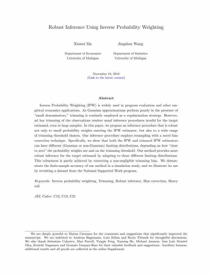
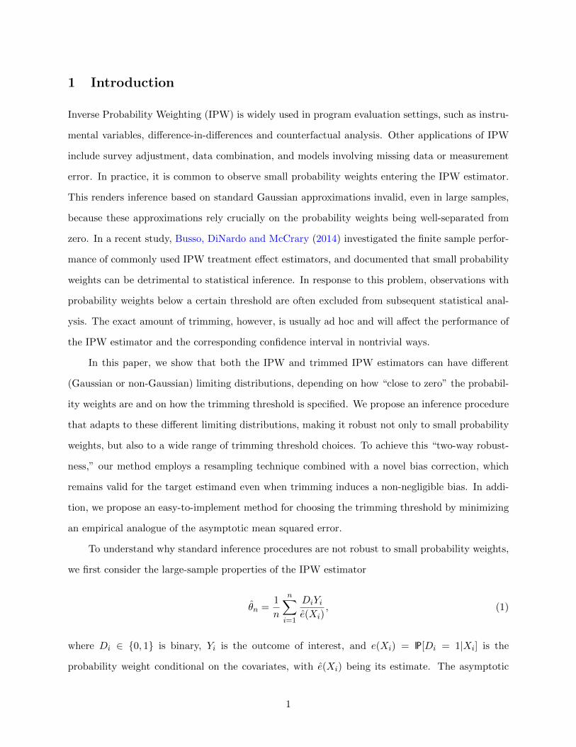
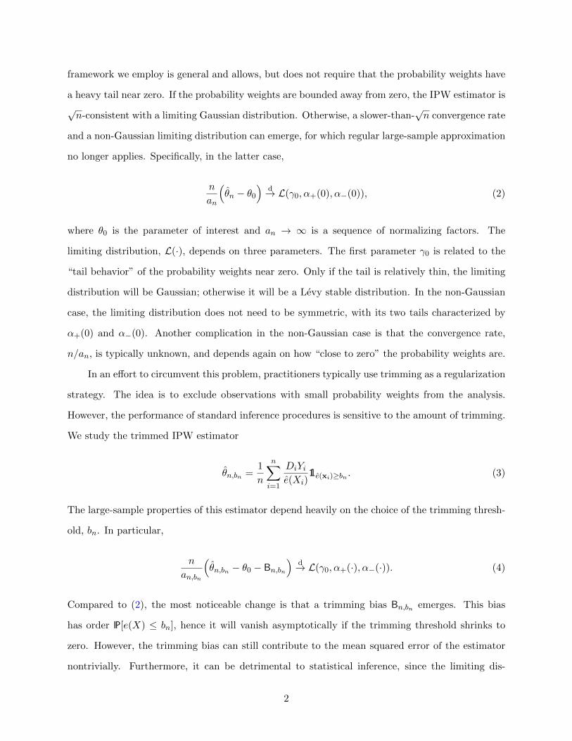

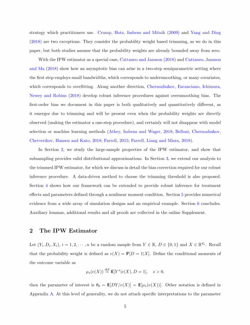

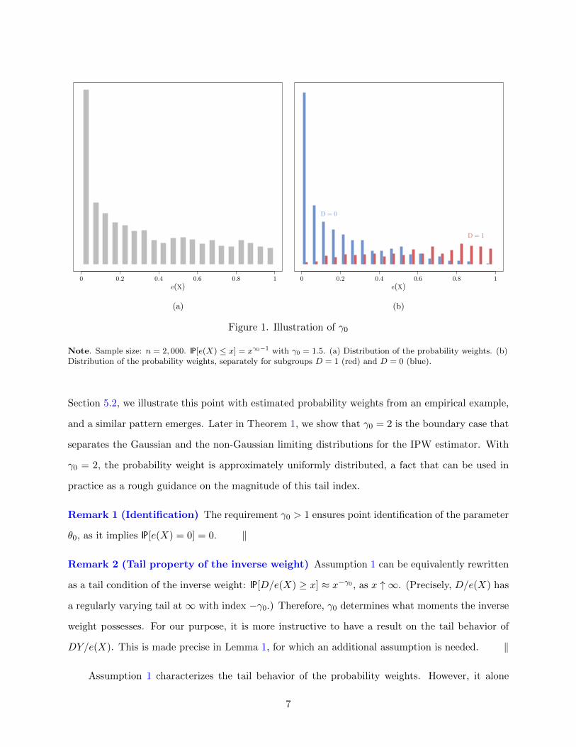
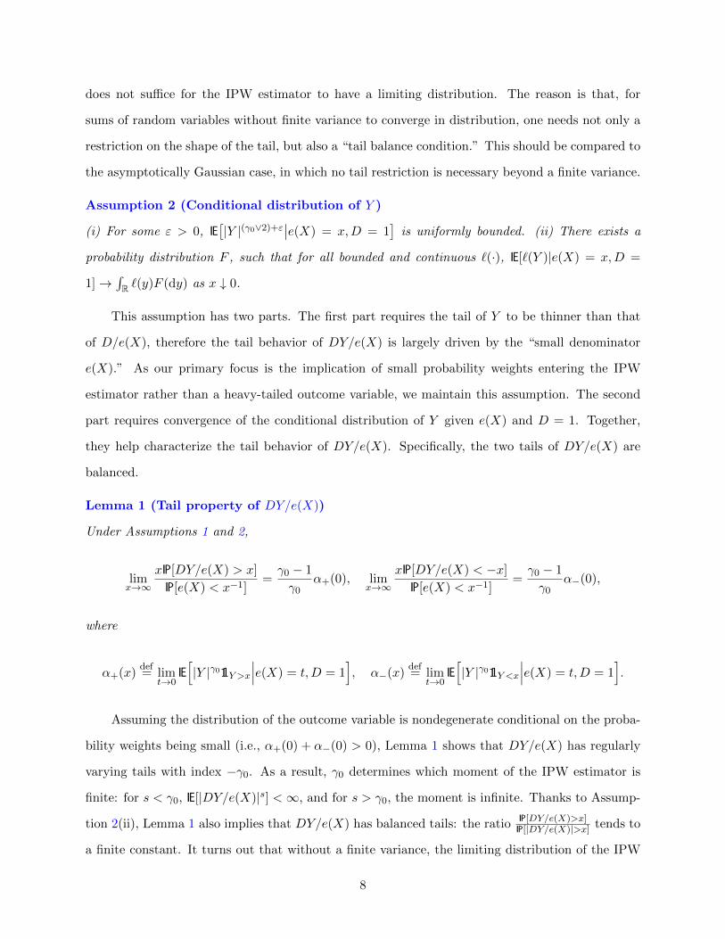
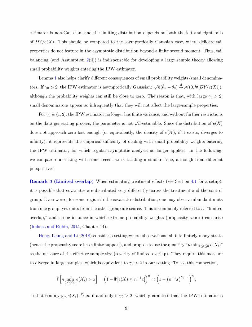
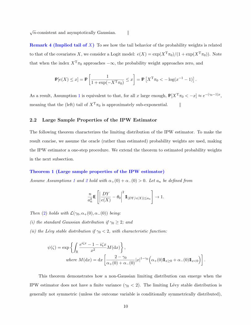


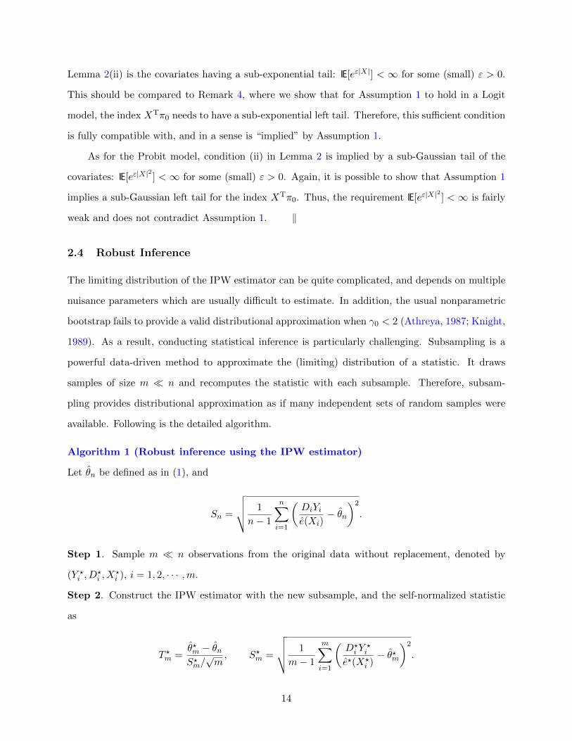
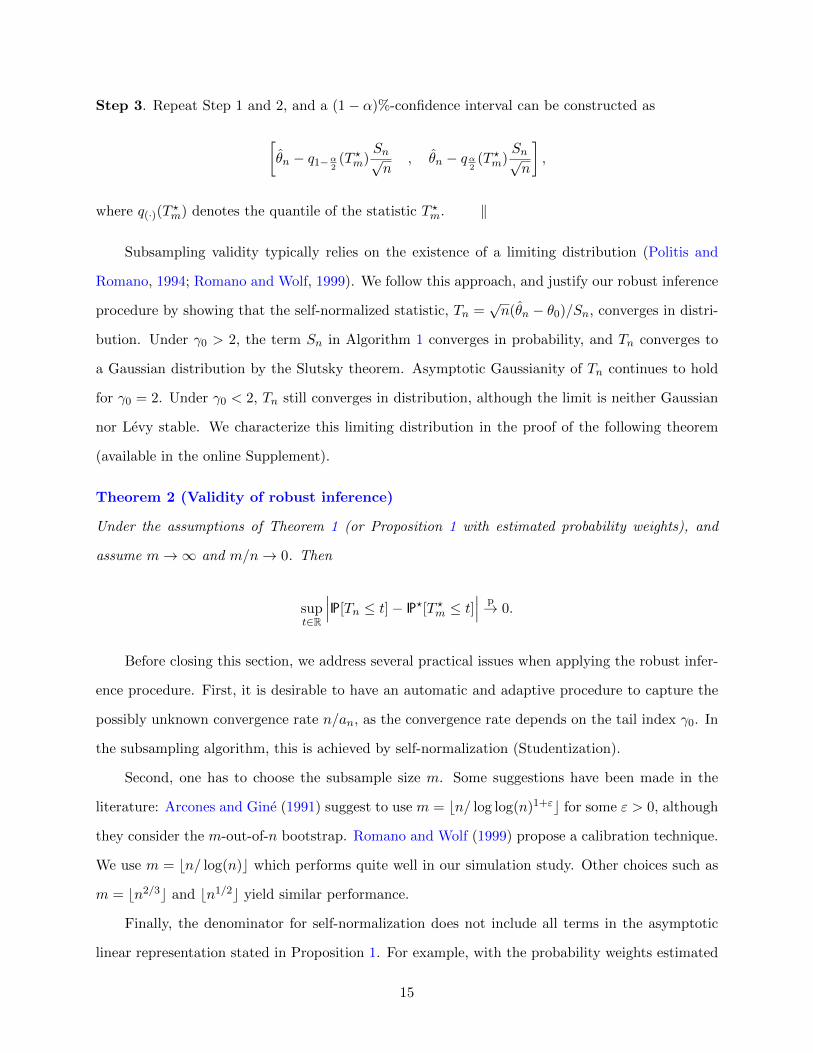

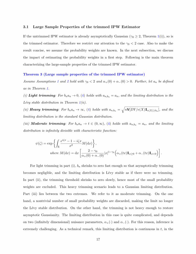
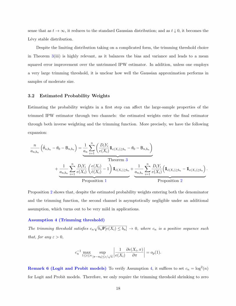
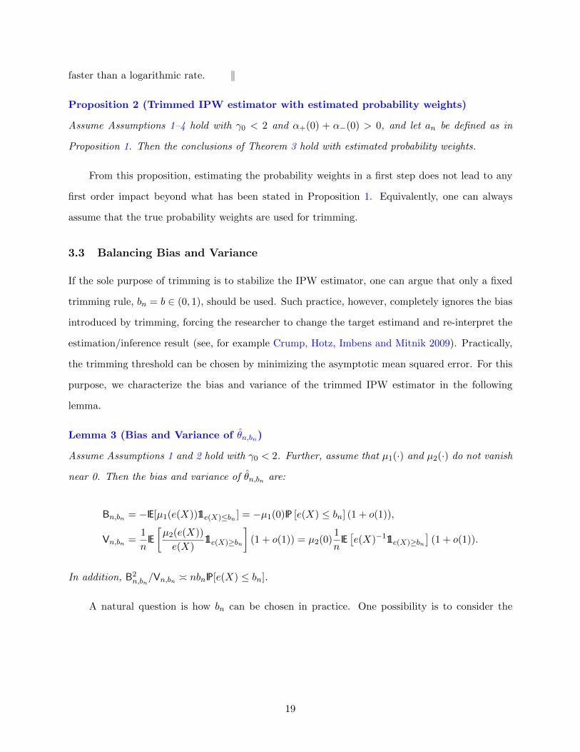
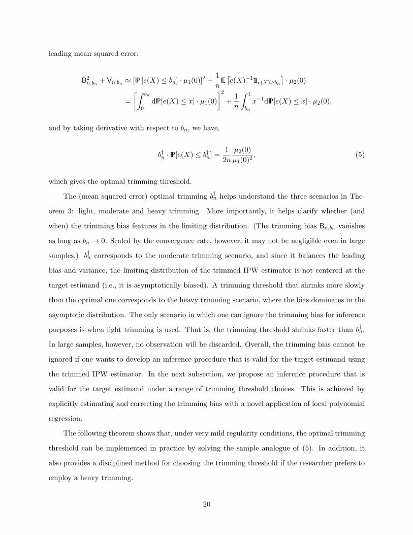


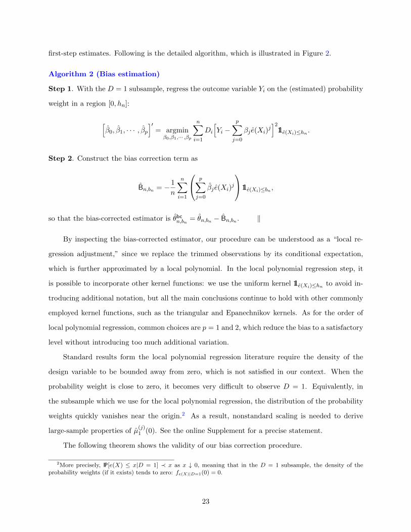


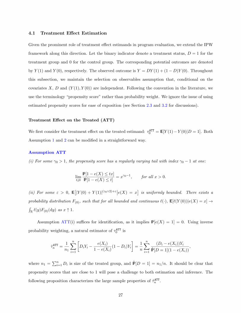
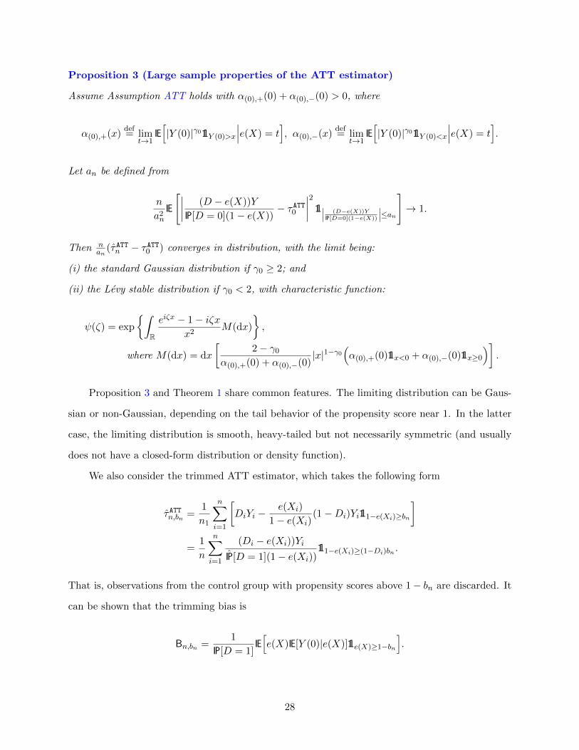

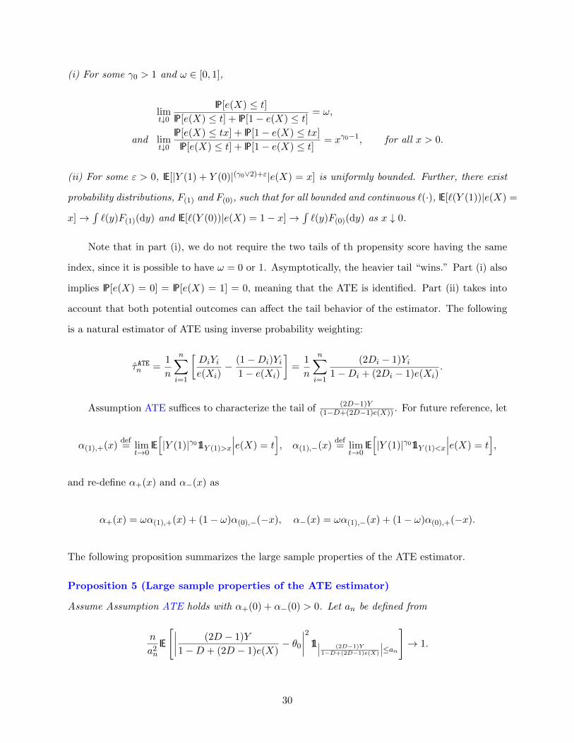
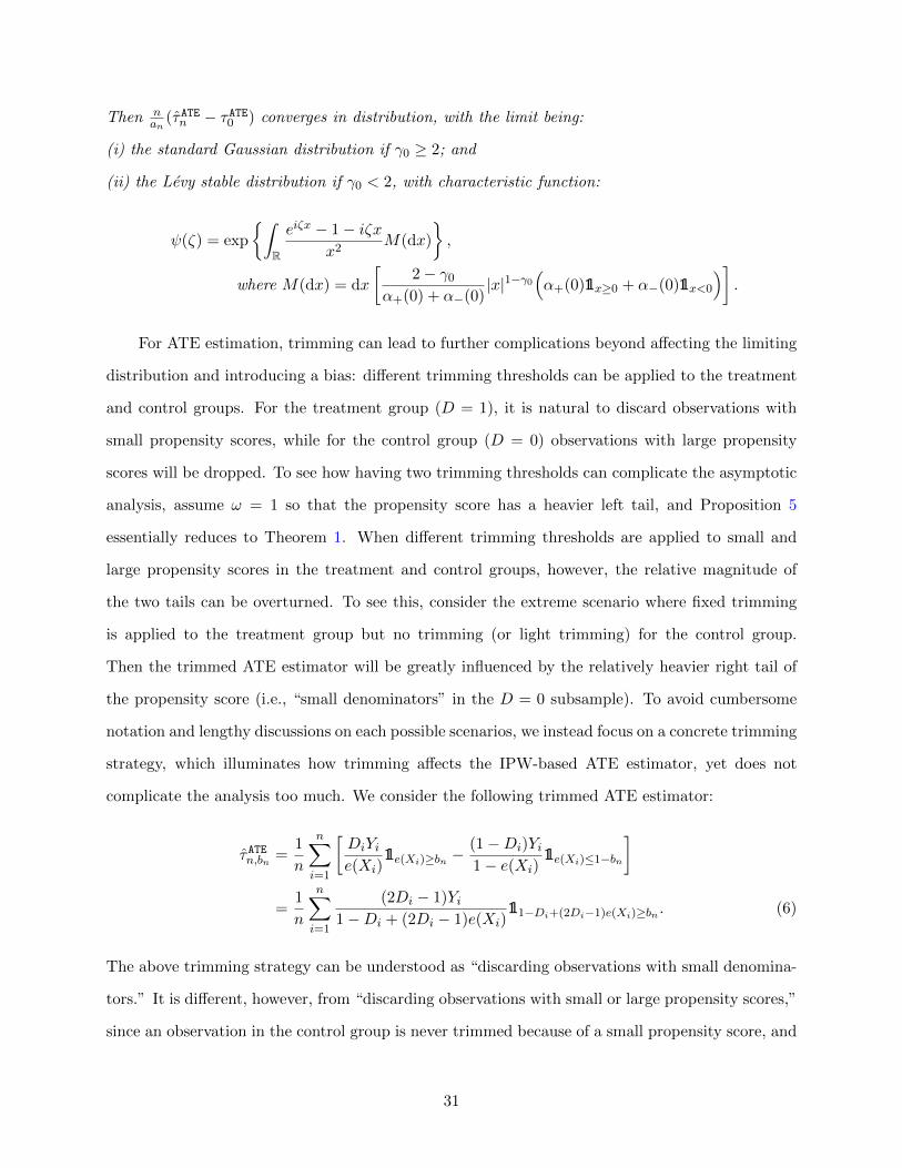
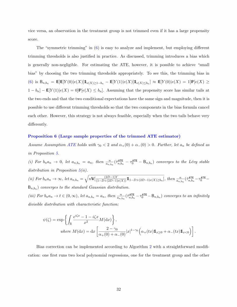


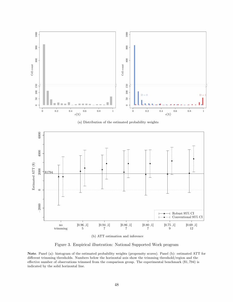
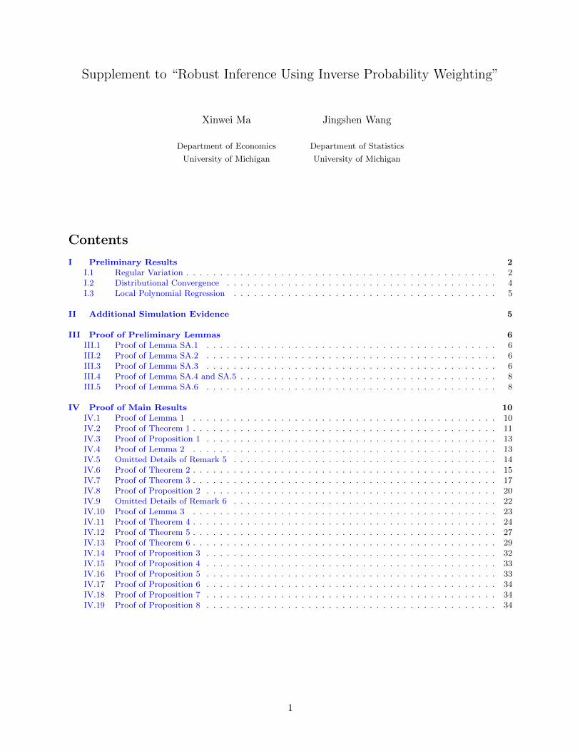

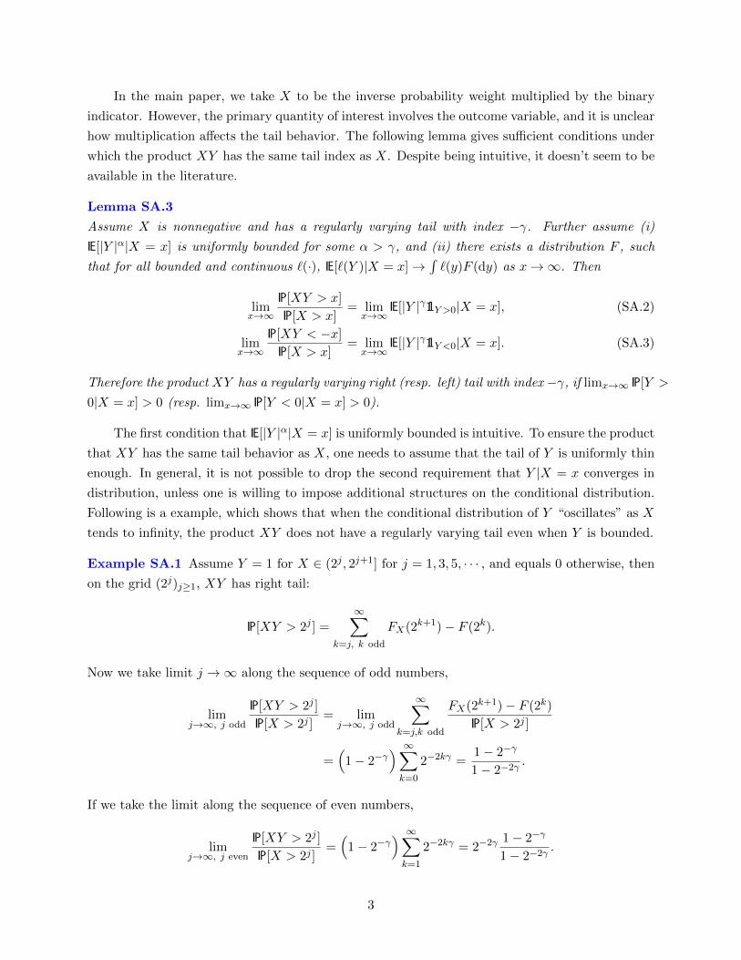


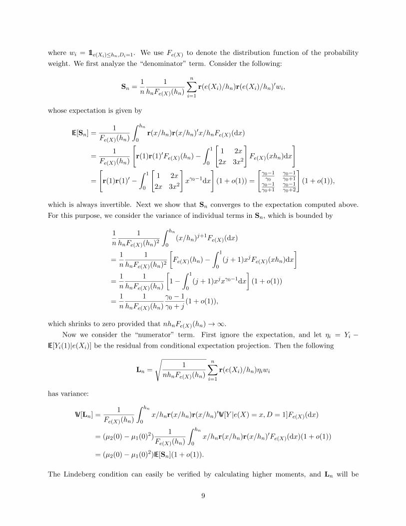


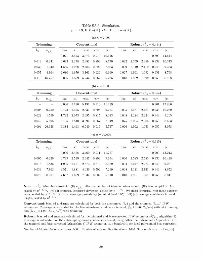


![SPECTRAL LIKELIHOOD EXPANSIONS FOR BAYESIAN INFERENCE · In view of inverse modeling [1, 2] and uncertainty quanti cation [3, 4], Bayesian inference establishes a convenient framework](https://static.documents.pub/doc/80x56/5f2241e5e36de465777028e4/spectral-likelihood-expansions-for-bayesian-inference-in-view-of-inverse-modeling.jpg)


