Robust Optimization with Multiple Ranges: Theory and

Application to R & D Project Selection

Ruken Duzgun∗ Aurelie Thiele†

July 2010

Abstract

We present a robust optimization approach when the uncertainty in objective coefficients

is described using multiple ranges for each coefficient. This setting arises when the value of

the uncertain coefficients, such as cash flows, depends on an underlying random variable, such

as the effectiveness of a new drug. Traditional robust optimization with a single range per

coefficient would require very large ranges in this case and lead to overly conservative results.

In our approach, the decision-maker limits the number of coefficients that fall within each

range; he can also limit the number of coefficients that deviate from their nominal value in a

given range. Modeling multiple ranges requires the use of binary variables in the uncertainty

set. We show how to address this issue to develop tractable reformulations and apply our

approach to a R&D project selection problem when cash flows are uncertain. Furthermore, we

develop a robust ranking heuristic, where the project manager ranks the projects according to

densities (ratio of cash flows to development costs) or Net Present Values, while incorporating

the budgets of uncertainty but without requiring any optimization procedure. While both

density-based and NPV-based ranking heuristics perform very well in experiments, the NPV-

based heuristic performs better; in particular, it finds the truly optimal solution more often.

Keywords: robust optimization; multiple ranges; project selection; robust ranking.

1 Introduction

Robust optimization addresses data uncertainty by assuming that uncertain parameters belong

to a bounded, convex uncertainty set and maximizing the minimum value of the objective over∗Department of Industrial and Systems Engineering, Lehigh University, Bethlehem, PA 18015,

rud207@lehigh.edu.†Department of Industrial and Systems Engineering, Lehigh University, Bethlehem, PA 18015, aure-

lie.thiele@lehigh.edu. Phone: +1-610-758-2903. Work supported in part by NSF Grant CMMI-0757983 andan IBM Faculty Award.

1

that uncertainty set, while ensuring feasibility for the worst-case value of the constraints. This

approach was pioneered by Soyster [27] in the 1970s; however, his model required that each

uncertain parameter be equal to its worst-case value, and thus was deemed too conservative for

practical implementation. In the mid-1990s, Ben-Tal and Nemirovski ([5, 6, 7]), El-Ghaoui and

Lebret [20] and El-Ghaoui et al. [21] presented tractable mathematical reformulations, based

on ellipsoidal uncertainty sets, that turned linear programming problems into second-order cone

problems and reduced the conservatism of Soyster’s [27] approach. Furthermore, Ben-Tal and

Nemirovski [8] studied robust optimization applied to conic quadratic and semidefinite program-

ming. Ben-Tal et. al. [4] provides an extensive book treatment of robust optimization with an

emphasis on ellipsoidal sets.

Bertsimas and Sim [12, 13] and Bertsimas et al. [11] investigated in the early 2000s the

special case where the uncertainty set is a polyhedron. Specifically, the uncertainty set consists

of range forecasts (confidence intervals) for each parameter and a constraint called a budget-

of-uncertainty constraint, which limits the number of coefficients that can take their worst-case

value. The approach preserves the degree of complexity of the problem (the robust counterpart

of a linear problem is linear) and allows the decision-maker to control the degree of conservatism

of the solution. Robust optimization remains the focus of substantial research efforts; recent

theoretical advances include the development of adjustable optimization (Ben-Tal et. al. [3])

and adaptable optimization (Bertsimas and Caramanis [10]) to incorporate information revealed

over time, while robust optimization has been successfully applied to a variety of areas, from

inventory management (Bertsimas and Thiele [15]) to revenue management (Adida and Perakis

[1]) to wireless sensor networks (Ye and Ordonez [29]). The reader is referred to Bertsimas et. al.

[9] for a comprehensive review paper and to Duzgun and Thiele [18] for an overview of dynamic

models in robust optimization.

In this paper, we focus on problem setups where the ranges taken by uncertain coefficients

depend on the realizations of underlying random variables. This problem arises for instance in

R&D project selection, where project cash flows are uncertain but also depend on the effec-

tiveness of the underlying compound tested by the pharmaceutical company. Project selection

requires binary variables, for which ellipsoidal uncertainty sets are ill-suited as they lead to non-

linear integer problems (Bertsimas and Sim [14]); therefore, we will focus throughout this paper

on polyhedral uncertainty sets, specifically, sets with range forecasts and budget-of-uncertainty

constraints. The traditional robust optimization approach, with a single range for each uncertain

coefficient, would require very large ranges and thus lead to overly conservative solutions. The

multi-range robust optimization approach we propose allows for a more realistic description of

2

uncertainty. While Metan and Thiele [25] introduces multiple ranges for product demand in

a simple two-stage robust revenue management problem for a single product, that approach is

an hybrid between robust optimization and stochastic programming, where the decision-maker

gains advance knowledge of the range that product demand will fall into. It incorporates neither

binary variables nor budgets of uncertainty and has a single source of uncertainty, and focuses

on the impact of scenario probabilities on the quality of the optimal solution. Bienstock [16]

incorporates multiple ranges to classical mean-variance problems in portfolio management. In

that framework, risk is discretized by constructing uncertainty “bands” around estimates of the

return shortfalls of the assets; observations in the same band represent similar levels of risk.

The user specifies rough estimates of the frequencies with which shortfalls fall within each band,

and constructs intervals for the actual number of occurrences in the bands, leading to a his-

togram model. The proposed model is solved using a cutting-plane algorithm with a convex

master problem (called the implementor problem) and a mixed-integer subproblem (called the

adversarial problem), which generates cuts for the implementor problem. The results suggest

that the cutting-plane algorithm implemented can successfully address uncertainty models with

non-convexities for large-scale problems and is of interest in applications beyond finance.

The Research and Development (R&D) project selection problem has been studied since the

1960s. Competition between R&D companies has increased the importance of funding projects

that would best meet their needs. While many methods to identify these projects have been

investigated, there is no consensus on their practical effectiveness. Martino [24] presents various

methods available for selecting R&D projects, in particular ranking methods, economic models,

portfolio or optimization models and ad-hoc methods.

Early studies of the R&D project selection problem mostly use ranking methods. The most

common ones are scoring models and the analytic hierarchy procedure (AHP) (see Baker and

Freeland [2] for a literature review on these approaches.) Economic methods, which are recom-

mended by Martino [24], consider the cash flows involved with the project, using metrics such

as net present value (NPV), internal rate of return (IRR) and cash flow payback. Portfolio opti-

mization methods implement mathematical programming to find the projects, from a candidate

project list, that would give the maximum payoff to the firm. For instance, Childs and Triantis

[17] use a real options framework in order to examine dynamic R&D investment policies and

valuation of R&D programs, and Stummer and Heidenberger [28] use a multi-objective integer

programming model to determine all efficient (Pareto-optimal) portfolios.

Data envelopment analysis (DEA) is another method for solving R&D project selection de-

cisions. Linton et. al [23] proposed this method to split decisions on project portfolios into

3

accept, consider-further and reject sub-groups. Eilat et. al [19] use a methodology based on an

extended DEA that quantifies some qualitative concepts embedded in the balanced scorecard

(BSC) approach. They employ a DEA-BSC model first to evaluate individual R&D projects,

and then to evaluate alternative R&D portfolios.

R&D project selection problems include high levels of uncertainty in future cash flows; how-

ever, the most common approaches to project selection replace uncertain parameters by their

expected values or rely on traditional, stochastic descriptions of randomness, although quanti-

fying accurately the probability distributions of future cash flows for a R&D project and the

probabilities of project success is very difficult in practice. As mentioned above, the classical

robust optimization approach also suffers from over-conservatism in this setup due to the large

ranges that would be required to implement it. This makes multi-range robust optimization a

novel theoretical extension of robust optimization with valuable practical applications.

Contributions. Our contributions to the literature are as follows.

• We define the multi-range robust optimization framework and derive tractable reformula-

tions.

• In particular, we show that the linear relaxation of the worst-case problem (which computes

the worst-case objective for a given strategy and requires binary variables to model multiple

ranges) has integer optimal solutions in both robust optimization models we consider.

• We apply the approach to a R&D project selection problem.

• We present a robust ranking heuristic to identify projects to fund without any optimization

and test it in numerical experiments.

• Our computational results suggest that, in this setting, ranking projects according to Net

Present Values rather than densities (ratio of cash flows to development costs), yields

higher-quality solutions, i.e., solutions closer to optimality.

To the best of our knowledge, we are the first to incorporate the idea of robust ranking to a

range- and budgets-of-uncertainty-based description of uncertainty.

Outline. Section 2 introduces the generic multi-range robust optimization approach. In Section

3, we apply our methodology to a R&D project selection problem. Section 4 introduces heuristics

based on robust ranking. Numerical results are presented in Section 5. Finally, Section 6 contains

concluding remarks.

4

2 Multi-Range Robust Optimization

We first provide a quick overview of traditional (one-range) robust optimization before discussing

its limitations and presenting the approach with multiple ranges.

2.1 Review of One-Range Robust Optimization

Let c be the objective coefficient vector of size n. The general model we consider is:

max c′x

s.t. x ∈ X ,(1)

where X is the constraint set of x, which may include integrality constraints. We further assume

that all decision variables are non-negative, which is a natural assumption to make in the context

of operations management, where decision variables represent for instance ordering quantities

or amounts transported; this assumption is particularly justified in the project management

application described in Section 3, where decision variables are binary.

We consider the case where the vector c is uncertain, which will correspond to uncertain

project cash flows in Section 3. We can apply the traditional one-range robust optimization ap-

proach that Bertsimas and Sim developed in [11], [13] to the uncertain parameter c. Specifically,

we model ci, i = 1, . . . , n, as an uncertain parameter in the interval [ci − ci, ci + ci]. (Note that,

since decision variables are non-negative, the worst case will always be achieved at the low end

of the range; therefore, knowledge of the high end of the range is not required to implement the

approach and the confidence interval does not have to be symmetric.) Define the scaled deviation

yi such that ci = ci + ci yi for all i. In line with Bertsimas and Sim [13], the scaled deviations

are assumed to belong to the polyhedral uncertainty set:

P = {y|n∑

i=1

|yi| ≤ Γ, |yi| ≤ 1, ∀i}.

The parameter Γ ∈ [0, n] is the budget of uncertainty which specifies the maximum number of

coefficients that can deviate from their nominal values.

• If Γ = 0, the only feasible element in P is the zero vector, so that the problem reduces to

its deterministic counterpart.

• If Γ = n, each uncertain parameter takes its worst case value.

• Taking a value of Γ between 0 and n allows the decision-maker to achieve a trade-off

5

between the nominal performance of the deterministic model and the risk protection of the

most conservative model.

While the setup above assumes that the project cash flows are independent, it is straightforward

to extend the approach to the case where cash flows are correlated by using the multi-factor

model described in Bertsimas and Sim [13]. This extension is left to the reader.

The robust problem becomes:

max minn∑

i=1

(ci + ci yi) xi

s.t. y ∈ Ps.t. x ∈ X .

(2)

Theorem 2.1 (One-range robust optimization (Bertsimas and Sim [13])). The robust counterpart

of Problem (1) is:

maxn∑

i=1

ci xi − Γz0 −n∑

i=1

zi

s.t. x ∈ Xzi + z0 ≥ ci xi, ∀i,zi, z0 ≥ 0 ∀i.

(3)

Proof. This is a direct application of Bertsimas and Sim [13] to Problem (2) after injecting the

fact that the worst case is always achieved for yi ≤ 0 for all i and that the decision vector x is

non-negative.

Limitations of the One-Range Framework. This framework is not well-suited for cases

where the uncertain parameters are driven by underlying random variables. For instance, in

the case of drug trials, the potential revenue of a drug will depend on the effectiveness of the

active chemical compound being tested; if the performance of the compound is disappointing,

the resulting cash flows will fall in a low range; if the compound is effective in healing a wide

array of patients, cash flows will fall in a high range. Trying to encompass all possible values

of the cash flows into a single interval will generate an overly large range forecast, with an ill-

defined nominal value lacking any realistic meaning if it falls between the two intervals, as the

decision-maker never believes he will observe such cash flows.

This is particularly a concern in robust optimization, since it can be shown (see Bertsimas

and Sim [13]) that at optimality, the worst-case coefficients of Problem (2) will be equal to either

their worst case or their nominal value, assuming the budget of uncertainty is integer. Hence, it is

6

important for the relevance of the robust optimization approach and its adoption by practitioners

that the optimal values of the uncertain coefficients correspond to values these parameters can

actually take. Similar arguments can be made in the case of demand for a new product, the

sales of which depends on the degree of popularity or market share that the product will achieve.

Such items, with a wide range of possible outcomes, require a finer-grained representation of

uncertainty than the one-range model is able to provide.

2.2 The Case With Multiple Ranges

Instead of having a single range of uncertainty, we now assume that we have multiple ranges

that the uncertain values can take values from. For notational simplicity, we assume that each

uncertain parameter has the same number m of possible ranges, but the approach can be extended

easily to the case where the number of ranges depends on the uncertain parameter. We will

analyze two cases:

1. The simple case where the (pessimistic) decision-maker assumes that each uncertain param-

eter takes the worst value of the range it falls into, and the maximum number of parameters

that can fall in a given range is bounded by a budget of uncertainty.

2. The more complex case where the decision-maker extends the setup in Case 1 to introduce

another family of budgets of uncertainty limiting the number of parameters that can take

their worst-case value in a given range. This allows some parameters to be equal to their

nominal value, rather than their worst-case value, in that range.

2.2.1 Case 1: Without a Budget For the Deviations Within The Ranges

Let ck−i , resp. ck+

i be the lower, resp. higher, bound of range k for parameter i, i = 1, . . . , n,

k = 1, . . . ,m. The budget Γk constrains the maximum number of coefficients that can fall within

range k, k = 1, . . . , m. (The decision maker can also choose to introduce these budgets only for

the lowest ranges, corresponding to the most conservative outcomes, to limit the conservatism

of the approach.)

7

The robust problem can be formulated as a mixed-integer programming problem (MIP):

maxx∈X

minc,y

c′x

s.t. ck−i yk

i ≤ cki ≤ ck+

i yki , ∀i, k,

m∑

k=1

yki = 1, ∀i,

ci =m∑

k=1

cki , ∀i,

n∑

i=1

yki ≤ Γk, ∀k,

yki ∈ {0, 1}, ∀i, k.

(4)

The tractability of the robust optimization paradigm relies on the decision-maker’s ability to

convert the inner minimization problem into a maximization problem, of such a structure that the

master maximization problem (incorporating the outer maximization problem and the new inner

maximization problem) can be solved efficiently. Strong duality has emerged as the tool of choice

to implement this conversion (Bertsimas and Sim [13]); however, the model of uncertainty we

propose require the use of integer (binary) variables, which makes the rewriting of a minimization

problem as an equivalent maximization one considerably more difficult. It is thus natural to

investigate whether the linear relaxation of the inner minimization problem in Problem (4) yields

binary y variables at optimality. This is the purpose of Lemma 2.2.

Lemma 2.2. The linear relaxation of the inner minimization problem:

minc,y

c′x

s.t. ck−i yk

i ≤ cki ≤ ck+

i yki , ∀i, k,

m∑

k=1

yki = 1, ∀i,

ci =m∑

k=1

cki , ∀i,

n∑

i=1

yki ≤ Γk, ∀k,

yki ∈ {0, 1}, ∀i, k,

(5)

has a binary optimal vector y for any given integer Γl and nonnegative vector x.

Proof. The objective is a minimization over c of c′x where ci =m∑

k=1

cki for all i and x is non-

8

negative. Hence, cki will take the minimum value in its range, i.e., ck

i = ck−i yk

i at optimality for

all i, k. It follows that ci =m∑

k=1

ck−i yk

i for all i and the feasible set is reduced to∑m

k=1 yki = 1, ∀i,

∑ni=1 yk

i ≤ Γk, ∀k, and yki ∈ {0, 1}, ∀i, k,. The feasible set of the linear relaxation has binary

extreme points, thus proving the lemma.

This allows us to derive a tractable reformulation of Problem (4).

Theorem 2.3. Problem (4) has the equivalent robust linear formulation:

maxn∑

i=1

pi −m∑

k=1

γk Γk −n∑

i=1

m∑

k=1

zki

s.t. pi − γk − zki ≤ ck−

i xi, ∀i, k,

x ∈ Xγk, zk

i ≥ 0, ∀i, k.

(6)

Proof. As in the proof of Lemma 2.2, we notice that, due to the non-negativity of the vector x,

the optimal objective coefficients in the robust optimization framework are always achieved at

the low end of the range. Therefore, we can rewrite the group of constraints:

ck−i yk

i ≤ cki ≤ ck+

i yki , ci =

m∑

k=1

cki ,

as:

ci =m∑

k=1

ck−i yk

i .

We use Lemma 2.2 to rewrite Problem (5) as:

minc,y,u

n∑

i=1

m∑

k=1

ck−i yk

i xi,

s.t.m∑

k=1

yki = 1, ∀i,

n∑

i=1

yki ≤ Γk, ∀k,

0 ≤ yki ≤ 1, ∀i, k,

(7)

which is a linear programming problem with a non-empty, bounded feasible set. We can then

invoke strong duality to reformulate the minimization as a maximization problem, i.e., replace

the primal formulation by its dual. Re-injecting yields Problem (6).

9

2.2.2 Case 2: With a Budget For the Deviations Within the Ranges

In practice, it is unlikely that every single uncertain parameter will take the worst-case value of

the range it falls in. The purpose of this section is to extend the robust optimization approach

presented in Section 2.2.1 to the case where the manager also decides how many parameters, at

most, can take the worst-case value in the ranges they are in.

As before, the uncertain coefficients satisfy:

ci =m∑

k=1

cki , ∀i,

ck−i yk

i ≤ cki ≤ ck+

i yki , ∀i, k,

m∑

k=1

yki = 1, ∀i,

n∑

i=1

yki ≤ Γk, ∀k,

yki ∈ {0, 1}, ∀i, k.

Because we need to define the deviation of each parameter within its given range, we further

assume that the nominal value of parameter i in range k, denoted cki , is known for all i = 1, . . . , n

and k = 1, . . . ,m. The measure of uncertainty for parameter i of range k is then defined as

cki = ck

i − ck−i for all i = 1, . . . , n and k = 1, . . . ,m. Again, because the decision variables are

non-negative, the part of the range forecast above the nominal value will not be used in the

robust optimization approach and the optimal uncertain coefficients satisfy:

ci =m∑

k=1

(cki − ck

i zki ) yk

i ,

where zki is the scaled deviation of coefficient i, i = 1, . . . , n, from its nominal value in range k,

k = 1, . . . ,m with:n∑

i=1

m∑

k=1

zki ≤ Γ,

0 ≤ zki ≤ 1, ∀i, k.

Lemma 2.4. For any feasible x ∈ X , the worst-case objective can be computed as a mixed-integer

10

programming problem:

minc,y

n∑

i=1

m∑

k=1

xi

(cki yk

i − cki uk

i

)

s.t. uki ≤ yk

i , ∀i, k,n∑

i=1

m∑

k=1

uki ≤ Γ,

m∑

k=1

yki = 1, ∀i,

n∑

i=1

yki ≤ Γk, ∀k,

yki ∈ {0, 1}, ∀i, k,

uki ≥ 0, ∀i, k.

(8)

Proof. Defining uki = zk

i yki , we obtain:

cki = ck

i yki − ck

i uki , ∀i, k,

where 0 ≤ uki ≤ yk

i . The result follows from the fact that it is suboptimal to have zki > 0 when

uki = 0 for any i, k.

The following lemma is key to the tractability of the robust optimization approach we present.

Lemma 2.5. The constraint matrix of Problem (8) is totally unimodular.

Proof. A matrix obtained by a pivot operation on a totally unimodular matrix is totally uni-

modular (Nemhauser and Wolsey [26]). The matrix C below is the constraint matrix of Problem

(8) where the columns represent the variables [u y].

C =

Inm −Inm

11×nm 01×nm

0m×nm An×nm

0n×nm Bm×nm

where Inm is the nm× nm identity matrix and matrix An×nm has the following structure:

1 · · · 1 0 · · · 0 · · · 0 · · · 0

0 · · · 0 1 · · · 1 · · · ......

. . ....

0 · · · 0 · · · 1 · · · 1

11

Specifically, A is defined as:

Ai,j =

1 if (i− 1)m < j ≤ im

0 otherwise,

Matrix Bm×nm has the following structure:

1 · · · 0 1 · · · 0 · · · 1 · · · 0...

. . ....

.... . .

... · · · .... . .

...

0 · · · 1 0 · · · 1 · · · 0 · · · 1

Specifically, B has the following structure:

B =(Im×m Im×m · · · Im×m

)

We will do the following operations on C.

1) Let Rj is the jth row and Rj is the jth column of C. By doing the row operations, we obtain

the r-th version of the matrix C which is denoted by (C)r

For j = nm + 2 to nm + 2 + m, do

−Rj + Rnm+1 → Rnm+1

and call the resulting matrix (C)m.

Now, for j = 1 to nm, do

Rj + Rj+nm → Rj+nm.

and call the resulting matrix (C)m(n+1).

2) At the end of these row/colum operations we obtain the matrix (C)m(n+1), which is

(C)m(n+1) =

Inm 0nm

11×nm 01×nm

0m×nm An×nm

0n×nm Bm×nm

To conclude the proof, we will need the following result.

12

Lemma 2.6. (Nemhauser and Wolsey [26], p. 544) Let A be a (0, 1,−1) matrix with no more

than two nonzero elements in each column. Then A is totally unimodular if and only if the rows

of A can be partitioned into two subsets Q1 and Q2 such that if a column contains two nonzero

elements, the following statements are true:

a. If both nonzero elements have the same sign, then one is in a row contained in Q1 and

the other is in a row contained in Q2.

b. If the two nonzero elements have opposite sign, then both are in rows contained in the

same subset.

The matrix (C)m(n+1) satisfies these conditions of total unimodularity. Since a matrix ob-

tained by pivot operations on a totally unimodular matrix is also totally unimodular, our con-

straint matrix C is totally unimodular.

Theorem 2.7. The robust counterpart is equivalent to the following problem, with a linear

objective and linear constraints added to the original feasible set:

maxn∑

i=1

pi −n∑

i=1

m∑

k=1

zki −

m∑

k=1

γk Γk − Γ γ0

s.t. πki + γ0 ≥ ck

i xi, ∀i, k,

πki + pi − γk − zk

i ≤ cki xi, ∀i, k,

x ∈ Xγk, γ0, π

ki , zk

i ≥ 0 ∀i, k.

(9)

Proof. Since the constraint matrix of Problem (8) is totally unimodular (Lemma 2.5) and the

right-hand-side values of the constraints are integer, the linear relaxation of the problem has

integer optimal solutions. It follows from strong duality, because the feasible set of the linear

relaxation of Problem (8) is non-empty and bounded, that Problem (8) and the dual of its linear

relaxation have the same optimal objective. Reinjecting the dual yields Problem (9).

3 Application to Project Management

3.1 Problem Setup

We now apply the setting described in Section 2 to an example in R&D project selection. The

manager must decide in which projects to invest over a finite time horizon. Each project has

known cash requirements at each stage of its development (for notational simplicity, we assume all

13

projects have the same number of stages; this corresponds for instance to the case of drug trials of

small, medium and large scale leading to possible approval by the Food and Drug Administration

in the United States), but cash flows during and at the end of development are uncertain and

depend on underlying random variables, such as the effectiveness of the active compounds or

the market response to the new product. These random variables are realized only once (e.g.,

the drug compound is effective for the disease being treated), so that the coefficients for a given

project all fall in the low range or all fall in the high range. We allow for cash flows to be

generated during development as the company might file for patents or generate monetary value

from the results of the intermediary stages; the biggest cash flows, however, will be generated at

the end of the development phase.

We assume that there are two uncertainty ranges for each cash flow: a project might be

successful and has high cash flows, or it might be a failure and has low cash flows. Note that

cash flows are non-zero, even in the low state, as the drug might be found to be effective on a

subset of the patients and retain some market value. Because no new information is revealed

during the time horizon in this robust optimization setting, we do not consider the possibility of

stopping a project after it has started, before the end of the development phase.

The goal is to maximize the worst-case cumulative Net Present Value of the projects the

manager invests in, where the worst case is computed over the uncertainty sets described in

Sections 2.2.1 and 2.2.2, subject to constraints on the amount of money available at each time

period to spend on development. We will use the following notation throughout the paper.

General and cost parameters.n : number of projects,

T : number of time periods,

S : number of development phases for each project,

Bt : available budget for the time period t where t = 1,..., T ,

CDi,s : development cost of project i in phase s,

r : discount rate at each time period.Cash flow parameters.

14

CF l−i,s : lower bound of cash flow of project i in phase s if the project is unsuccessful,

CFli,s : nominal value of the cash flow of project i in phase s if the project is unsuccessful,

CF l+i,s : upper bound of cash flow of project i in phase s if the project is unsuccessful,

CFl

i,s : measure of uncertainty for cash flow of project i in phase s in low range (= CFli,s − CF l−

i,s ),

CF h−i,s : lower bound of cash flow of project i in phase s if the project is successful,

CFhi,s : nominal value of the cash flow of project i in phase s if the project is successful,

CF h+i,s : upper bound of cash flow of project i in phase s if the project is successful,

CFh

i,s : measure of uncertainty for cash flow of project i in phase s in high range (= CFhi,s − CF h−

i,s ),

Robust optimization parameters and decision variables.Γl : uncertainty budget that restricts the number of projects whose cash flows will be

in the low range,

Γ : uncertainty budget that restricts the number of projects whose cash flows deviate from

their nominal value within their given range,

xi,τ : 1 if the project i is selected to begin at time τ , 0 otherwise,

yi : 1 if the project i is in its low range (unsuccessful), 0 otherwise.

The deterministic project selection problem where each project can be selected at most once is

formulated as:

maxn∑

i=1

T−S+1∑

τ=1

xi,τ

(1 + r)τ−1

[S∑

s=1

CFi,s

(1 + r)s

]

s.t.n∑

i=1

t∑

τ=max{1,t−S+1}CDi,t−τ+1 xi,τ ≤ Bt ∀t

T∑

τ=1

xi,τ ≤ 1,

xi,τ ∈ {0, 1}, ∀i, τ.

(10)

3.2 Case 1: Robust Optimization Without a Budget for the Deviation Within

the Ranges

First, we consider the simple case where the manager only limits the number of projects that will

be unsuccessful, and assumes that each cash flow will take its worst case within a given range.

15

Problem (4) becomes:

maxx

minCFi,s,yi

n∑

i=1

T−S+1∑

τ=1

xi,τ

(1 + r)τ−1

[S∑

s=1

CFi,s

(1 + r)s

]:Total cash flow over time

s.t. CF l−i,s yi ≤ CF l

i,s ≤ CF l+i,s yi ∀(i, s) :Cash flow interval if in low range

CF h−i,s (1− yi) ≤ CF h

i,s ≤ CF h+i,s (1− yi) ∀(i, s) :Cash flow interval if in high range

CF li,s + CF h

i,s = CFi,s ∀(i, s) :Cash flow is either high or lown∑

i=1

yi ≤ Γl :At most Γl projects in low range

yi ∈ {0, 1}, ∀iCF l

i,s, CF hi,s, CFi,s ≥ 0 ∀(i, s)

s.t.n∑

i=1

t∑

τ=max{1,t−S+1}CDi,t−τ+1 xi,τ ≤ Bt ∀t :Budget constraint at each time period

T∑

τ=1

xi,τ ≤ 1, ∀(i) :Each project started at most once

xi,τ ∈ {0, 1}, ∀i, τ.(11)

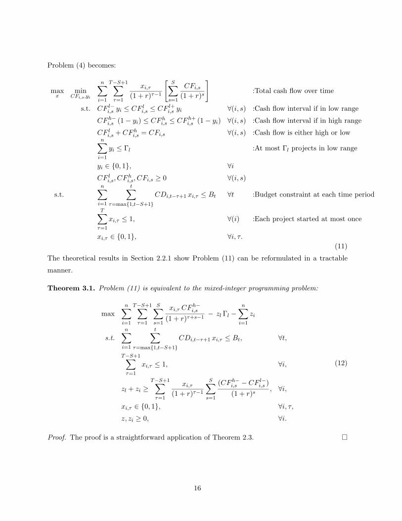
The theoretical results in Section 2.2.1 show Problem (11) can be reformulated in a tractable

manner.

Theorem 3.1. Problem (11) is equivalent to the mixed-integer programming problem:

maxn∑

i=1

T−S+1∑

τ=1

S∑

s=1

xi,τ CF h−i,s

(1 + r)τ+s−1− zl Γl −

n∑

i=1

zi

s.t.n∑

i=1

t∑

τ=max{1,t−S+1}CDi,t−τ+1 xi,τ ≤ Bt, ∀t,

T−S+1∑

τ=1

xi,τ ≤ 1, ∀i,

zl + zi ≥T−S+1∑

τ=1

xi,τ

(1 + r)τ−1

S∑

s=1

(CF h−i,s − CF l−

i,s )(1 + r)s

, ∀i,

xi,τ ∈ {0, 1}, ∀i, τ,z, zi ≥ 0, ∀i.

(12)

Proof. The proof is a straightforward application of Theorem 2.3.

16

3.3 Case 2: Robust Optimization With a Budget for the Deviation Within

the Ranges

Assume that cash flows for project i in phase s, with i = 1, . . . , n, s = 1, . . . , S, are either in

[CFli,s − CF

l

i,s, CFli,s + CF

l

i,s] or [CFhi,s − CF

h

i,s, CFhi,s + CF

h

i,s]. In line with the framework in

Section 2.2.2, they can be written in mathematical terms as:

CFi,s = (CFli,s − CF

l

i,s zli,s)y

li + (CF

hi,s − CF

h

i,s zhi,s)y

hi ,

with 0 ≤ zli,s, z

hi,s ≤ 1 ∀i, s and yj

i ∈ {0, 1} ∀j ∈ {l, h}. Since the coefficients must belong to

one of the two ranges, we only introduce a budget-of-uncertainty constraint on the number of

coefficients that fall into their low range.

Given feasible binary variables xi,τ (equal to 1 if project i is started at time τ and 0 otherwise),

the worst-case cash flows are given by:

minul,uh,y

n∑

i=1

T−S+1∑

τ=1

xi,τ

(1 + r)τ−1

S∑

s=1

CFli,s yl

i − CFl

i,s uli,s + CF

hi,s yh

i − CFh

i,s uhi,s

(1 + r)s

s.t. uli,s ≤ yl

i, ∀i, s,uh

i,s ≤ yhi , ∀i, s,

yli + yh

i = 1, ∀i,n∑

i=1

yli ≤ Γl,

n∑

i=1

S∑

s=1

(uli,s + uh

i,s) ≤ Γ,

yji ∈ {0, 1}, ∀i, ∀j ∈ {l, h},

uli,s, u

hi,s ≥ 0, ∀i, s.

(13)

It is a direct application of Lemma 2.5 that the constraint matrix of Problem (13) is totally

unimodular.

17

The robust optimization problem is given by:

maxx

minul,uh,y

n∑

i=1

T−S+1∑

τ=1

xi,τ

(1 + r)τ−1

S∑

s=1

CFli,s yl

i − CFl

i,s uli,s + CF

hi,s yh

i − CFh

i,s uhi,s

(1 + r)s

s.t. uli,s ≤ yl

i, ∀i, s,uh

i,s ≤ yhi , ∀i, s,

yli + yh

i = 1, ∀i,n∑

i=1

yli ≤ Γl,

n∑

i=1

S∑

s=1

(uli,s + uh

i,s) ≤ Γ,

yji ∈ {0, 1}, ∀i,∀j ∈ {l, h},

uli,s, u

hi,s ≥ 0, ∀i, s,

s.t.n∑

i=1

t∑

τ=max{1, t−S+1}CDi,t−τ+1 xi,τ ≤ Bt, ∀t,

T−S+1∑

τ=1

xi,τ ≤ 1, ∀i,

xi,τ ∈ {0, 1}, ∀i, τ.(14)

The following theorem provides a tractable reformulation of Problem (14). Because it is a

straightforward application of Theorem 2.7, we state it without proof.

Theorem 3.2. The robust optimization problem (14) is equivalent to the mixed-integer program-

18

ming problem:

maxn∑

i=1

pi −n∑

i=1

(zli + zh

i )− Γl γl − Γ γ0

s.t.n∑

i=1

t∑

τ=max{1,t−S+1}CDi,t−τ+1 xi,τ ≤ Bt, ∀t,

T−S+1∑

τ=1

xi,τ ≤ 1, ∀i,

S∑

s=1

πli,s + pi − γl − zl

i ≤T−S+1∑

τ=1

xi,τ

S∑

s=1

CFli,s

(1 + r)τ+s−1, ∀i,

S∑

s=1

πhi,s + pi − zh

i ≤T−S+1∑

τ=1

xi,τ

S∑

s=1

CFhi,s

(1 + r)τ+s−1, ∀i,

πli,s + γ0 ≥

T−S+1∑

τ=1

xi,τ CFl

i,s

(1 + r)τ+s−1, ∀i, s,

πhi,s + γ0 ≥

T−S+1∑

τ=1

xi,τ CFh

i,s

(1 + r)τ+s−1, ∀i, s,

xi,τ ∈ {0, 1}, ∀i, τ,πl

i,s, πhi,s ≥ 0 ∀i, s,

zli, z

hi ≥ 0, ∀i,

γl, γ0 ≥ 0.

(15)

The feasible set can be decomposed as follows:

• The first two groups of constraints are the same as in the deterministic model, representing

the maximum amount of money to be allocated at each time period and the fact that a

project can be started at most once.

• The third and fourth group of constraints are the dual constraints corresponding to the

primary variables yli and yh

i , respectively, and incorporate the information about the nomi-

nal values of the cash flows. Because one of these decision variables (either yli or yh

i ) will be

non-zero for each i at optimality, by complementarity slackness, one of the dual constraints

will be tight for each i, thus determining pi as a function of the nominal cash flow for that

range and the other dual variables. This will bring the nominal cash flows back into the

objective.

• The fifth and sixth group of constraints are the dual constraints corresponding to the

19

primary variables ulis and uh

is, respectively, and incorporate the information about the

uncertainty on the cash flows in each range. At most one of these decision variables (either

ulis or uh

is) will be non-zero for each i at optimality; if it is non-zero, by complementarity

slackness, one of the dual constraints will be tight for each i, thus determining either πlis or

πhis as a function of the uncertainty in that range and the other dual variables. (Otherwise

the πlis and πh

is variables will be at zero.) This will bring the cash flow uncertainty, through

the half-range of the confidence intervals, into the objective when needed.

• The other constraints are sign constraints or binary constraints.

The robust formulation (15) has n (3+T +2S)+2 decision variables and T +n(3+2S) constraints

in addition to sign and binary constraints; therefore, the size of the mixed-integer programming

problem increases linearly with each of the parameters n, T, S (number of projects, length of

time horizon, number of development stages) when the others are kept constant.

4 Robust Ranking Heuristic

While Problem (15) provides an exact formulation of the robust optimization problem for project

management, we focus in this section on developing optimization-free heuristics to provide a

feasible solution to the robust problem, which would give practitioners more insights into the

strategy they implement and the impact of the cash flow parameters.

We are motivated by the fact that, when there is only one time period and one development

phase (T = 1 and S = 1), the project selection problem has the structure of a knapsack problem,

for which a well-known heuristic is to rank items by decreasing order of density (value to weight

ratio) and fill the knapsack until the next item in the list does not fit (see, for instance, Kellerer

et. al. [22])). In particular, we provide a robust ranking procedure to rank the projects with

uncertain cash flows; to the best of our knowledge, we are the first to present such a ranking

procedure in the context of robust optimization.

We will consider two ways to rank the projects: (a) according to decreasing density, (b)

according to decreasing Net Present Value. Method (a) is motivated by its popularity to solve the

generic knapsack problem; Method (b) is motivated by its superior performance in the numerical

experiments provided in Section 5 and the widespread use of Net Present Value to select projects

in practice. Once projects are ranked, we apply the greedy multiple-knapsack heuristic described

in Kellerer et. al. [22] to generate a candidate solution. Specifically, we proceed down the ranked

list of projects and assign project j to knapsacks t, . . . , t+S− 1, with t the smallest integer such

that the project development costs fit in all of these knapsacks’ capacity.

20

4.1 Case 1: Ranking for the Projects Without a Budget for the Deviation

Within the Ranges

Recall that, if there is no budget for the deviation within the ranges, the cash flows always take

their worst case within the range, and that the range (high or low) is only selected once, i.e., the

range does not change with the development phase.

The high-level idea is to (i) compute two rankings, one using the low range of the cash flows

and the other using the high range, (ii) use the low-range ranking until the budget of uncertainty

has been used up, and then (iii) use the high-range ranking.

Ranking procedure.

Step 1 Compute the following parameters for all projects i.

Method (a): Densities

ahi =

S∑

s=1

CF h−i,s

(1 + r)s CDi,s

ali =

S∑

s=1

CF l−i,s

(1 + r)s CDi,s

Method (b): Net Present Values

ahi =

S∑

s=1

(−CDi,s +

CF h−i,s

(1 + r)s

)

ali =

S∑

s=1

(−CDi,s +

CF l−i,s

(1 + r)s

)

For either method, compute two rankings: in decreasing order of ahi , and in decreasing

order of ali.

Step 2 Add Γl projects to your ranking list corresponding to the projects with the largest Γl

values of ali. Then proceed to Step 3.

Step 3 Continue until all projects are ranked by choosing the unranked projects according to

the largest values of ahi , discarding projects that have already been selected in Step 2.

21

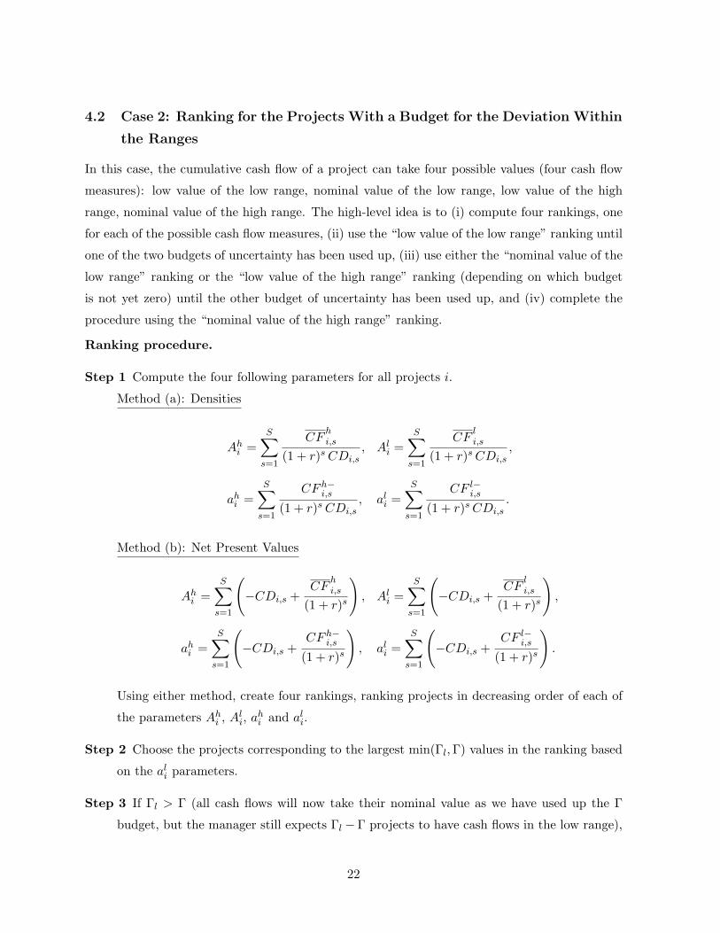
4.2 Case 2: Ranking for the Projects With a Budget for the Deviation Within

the Ranges

In this case, the cumulative cash flow of a project can take four possible values (four cash flow

measures): low value of the low range, nominal value of the low range, low value of the high

range, nominal value of the high range. The high-level idea is to (i) compute four rankings, one

for each of the possible cash flow measures, (ii) use the “low value of the low range” ranking until

one of the two budgets of uncertainty has been used up, (iii) use either the “nominal value of the

low range” ranking or the “low value of the high range” ranking (depending on which budget

is not yet zero) until the other budget of uncertainty has been used up, and (iv) complete the

procedure using the “nominal value of the high range” ranking.

Ranking procedure.

Step 1 Compute the four following parameters for all projects i.

Method (a): Densities

Ahi =

S∑

s=1

CFhi,s

(1 + r)s CDi,s, Al

i =S∑

s=1

CFli,s

(1 + r)s CDi,s,

ahi =

S∑

s=1

CF h−i,s

(1 + r)s CDi,s, al

i =S∑

s=1

CF l−i,s

(1 + r)s CDi,s.

Method (b): Net Present Values

Ahi =

S∑

s=1

(−CDi,s +

CFhi,s

(1 + r)s

), Al

i =S∑

s=1

(−CDi,s +

CFli,s

(1 + r)s

),

ahi =

S∑

s=1

(−CDi,s +

CF h−i,s

(1 + r)s

), al

i =S∑

s=1

(−CDi,s +

CF l−i,s

(1 + r)s

).

Using either method, create four rankings, ranking projects in decreasing order of each of

the parameters Ahi , Al

i, ahi and al

i.

Step 2 Choose the projects corresponding to the largest min(Γl, Γ) values in the ranking based

on the ali parameters.

Step 3 If Γl > Γ (all cash flows will now take their nominal value as we have used up the Γ

budget, but the manager still expects Γl − Γ projects to have cash flows in the low range),

22

add Γl − Γ projects to the ranked list by using the ranking based on the Ali parameters,

skipping the projects that have already been selected in Step 2.

Step 4 If Γ− Γl > 0, add Γ− Γl projects to the ranked list by using the ranking based on the

ahi parameters, skipping the projects that have already been selected in Steps 2 and 3.

Step 5 Continue until all projects are ranked by using the ranking based on the Ahi parameters,

skipping the projects that have already been selected in Steps 2, 3 and 4.

5 Numerical Example

In this section, we investigate the practical performance of our robust optimization models and

heuristics on an example. We focus on the case where T = 1 and S = 1, for which the mathe-

matical formulation without uncertainty becomes a well-known knapsack problem. Furthermore,

we consider two uncertainty ranges: high (indicated by the superscript h in relevant parameters)

and low (indicated by the superscript l). We have two main goals in this experiment:

1. Test whether the robust optimization framework does protect against downside risk as

advertised.

2. Test the performance of the heuristics, (a) compared to the optimal solution, (b) compared

to each other.

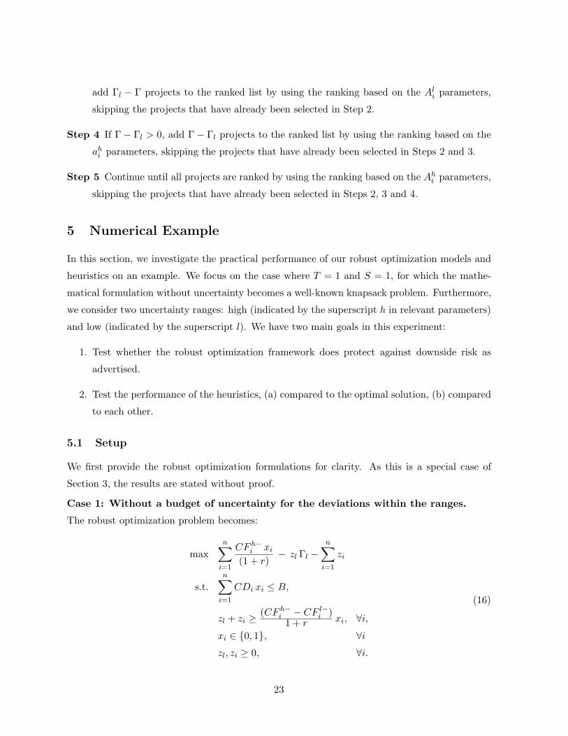
5.1 Setup

We first provide the robust optimization formulations for clarity. As this is a special case of

Section 3, the results are stated without proof.

Case 1: Without a budget of uncertainty for the deviations within the ranges.

The robust optimization problem becomes:

maxn∑

i=1

CF h−i xi

(1 + r)− zl Γl −

n∑

i=1

zi

s.t.n∑

i=1

CDi xi ≤ B,

zl + zi ≥ (CF h−i − CF l−

i )1 + r xi, ∀i,

xi ∈ {0, 1}, ∀izl, zi ≥ 0, ∀i.

(16)

23

The project density parameters (Method (a)) are given by:

Ahi = CF h−

i(1 + r)CDi

, Ali = CF l−

i(1 + r) CDi

.

The project Net Present Value parameters (Method (b)) are given by:

Ahi = −CDi + CF h−

i1 + r , Al

i = −CDi + CF l−i

1 + r .

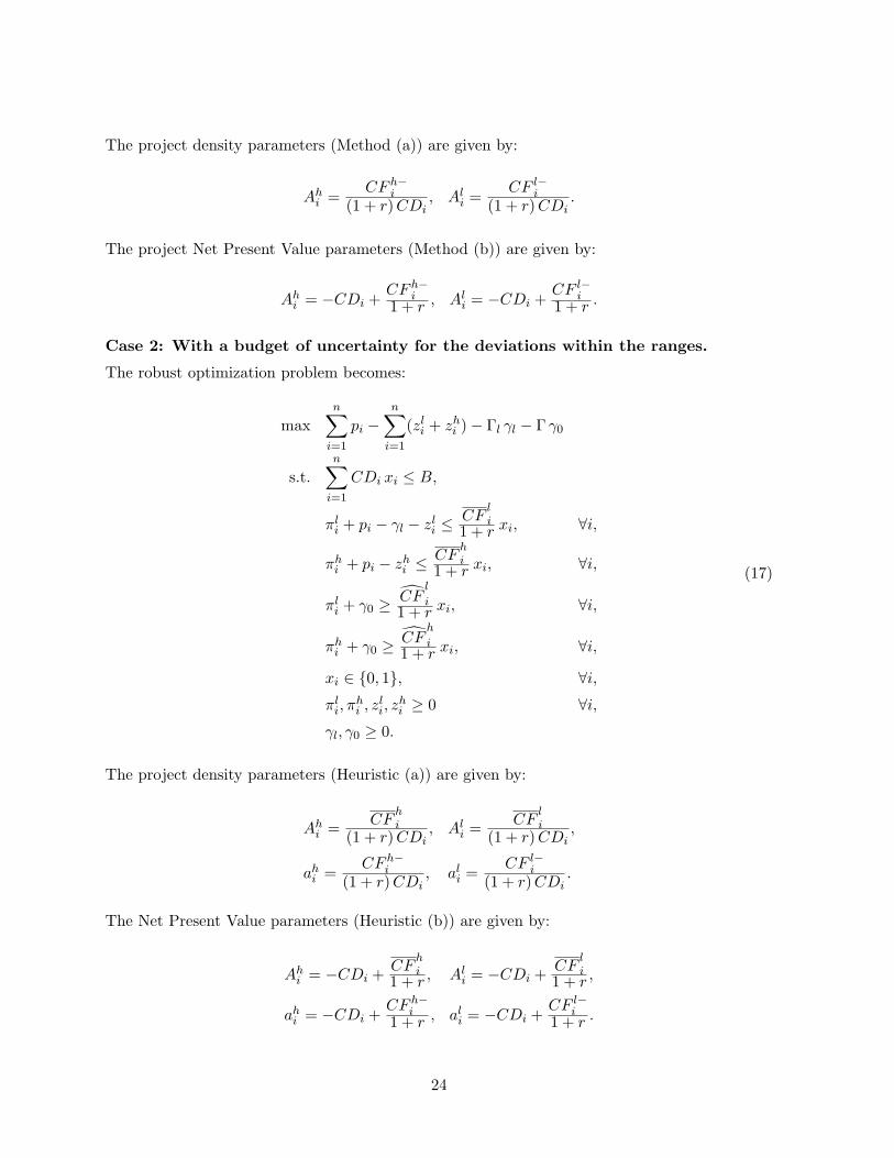
Case 2: With a budget of uncertainty for the deviations within the ranges.

The robust optimization problem becomes:

maxn∑

i=1

pi −n∑

i=1

(zli + zh

i )− Γl γl − Γ γ0

s.t.n∑

i=1

CDi xi ≤ B,

πli + pi − γl − zl

i ≤ CFli

1 + r xi, ∀i,

πhi + pi − zh

i ≤ CFhi

1 + r xi, ∀i,

πli + γ0 ≥ CF

l

i1 + r xi, ∀i,

πhi + γ0 ≥ CF

h

i1 + r xi, ∀i,

xi ∈ {0, 1}, ∀i,πl

i, πhi , zl

i, zhi ≥ 0 ∀i,

γl, γ0 ≥ 0.

(17)

The project density parameters (Heuristic (a)) are given by:

Ahi = CF

hi

(1 + r)CDi, Al

i = CFli

(1 + r) CDi,

ahi = CF h−

i(1 + r) CDi

, ali = CF l−

i(1 + r) CDi

.

The Net Present Value parameters (Heuristic (b)) are given by:

Ahi = −CDi + CF

hi

1 + r , Ali = −CDi + CF

li

1 + r ,

ahi = −CDi + CF h−

i1 + r , al

i = −CDi + CF l−i

1 + r .

24

5.2 Numerical Results

We tested our formulations and heuristics for 4 data sets. Data Sets 1 and 2 have 10 projects

while Data Sets 3 and 4 have 20 projects. In all cases, development costs (CDi) were generated

using a Uniform distribution in [80−120], nominal values of low cash flows (CFli) were generated

using Uniform distribution in (0.5 − 2.5) · CDi, and nominal values of high cash flows (CFhi )

generated using Uniform distribution in (2− 3.5) ·CDi. For all i, the deviation parameters CFl

i,

CFh

i were selected as 0.2 CFli, 0.2CF

hi respectively. Budget for development costs was set to

500 in all cases. In addition, Data Sets 3 and 4 were also solved for a value of the budget equal

to 1,000. The same distributions were used to compute the actual objective using random cash

flows once the optimization problem had been solved. The probability of the cash flows being in

the low range was taken equal to 0.5.

Optimal solution.

We solved Problem (15) for each data set and for each (Γ, Γl) combination. Figure 1 shows the

histogram of revenues for Data Set 1 and the deterministic model, where parameter values are

taken equal to their expected values, here (CFhi +CF

li)/2 for all i (red line with square markers)

as well as two robust models: (Γ, Γl) = (2, 1) and (Γ, Γl) = (3, 4) (blue line with lozenge markers

and green line with triangle markers, respectively). These budgets were chosen to have Γ > Γl

in one case and Γ < Γl in the other. This histogram was generated using 1,000 scenarios. Figure

1 suggests that robust optimization is more conservative than its nominal counterpart (limits

upside potential) but decreases the downside risk.

Figures 2 and 3 show the number of iterations versus budget of uncertainty Γl for five different

Γ values, for Data Sets 1 and 3, respectively. Recall that Data Set 1 has 10 projects and Data Set

3 has 20. (Our observations remain valid for other values of Γ, but the corresponding graphs were

omitted for graph readability.) We observe that, for each Γ value, the number of iterations in

the robust optimization models does not differ substantially from the number of iterations in the

deterministic model when Γl is close to its bounds (Γl = 0 or Γl = 10), which means that most

projects are in the same uncertainty range.) When projects are more evenly assigned to low and

high ranges (middle values of Γl), the number of iterations increases, sometimes substantially

(see Figure 3, where the top curve corresponds to Γ = 10).

Since robust optimization maximizes the worst-case cash flow over the uncertainty set, it

is natural to evaluate how well it protects against downside risk. To do that, we compute the

first and fifth percentile of the distribution of the random objective where we have injected the

optimal solution, for Data Set 1 and all (Γ, Γl) combinations, using 1,000 scenarios. These results

25

Figure 1: Histogram of Revenues.

Figure 2: Number of Iterations versus Budget of Uncertainties for Data Set 1, Budget=500.

are shown in Tables 1 and 2, respectively. Table 3 shows the expected value of the objective

for reference. We see that robust optimization does indeed protect against downside risk, as

evidenced in the increase in the values for the first and fifth percentile, with modest performance

degradation (decrease in average objective value).

It is important to note that the optimal solution will not change once Γ or Γl increases past

26

Figure 3: Number of Iterations versus Budget of Uncertainties for Data Set 3, Budget=1000.

the number of projects being funded, which we will denote x. If p is the (estimated) probability of

project cash flows falling in the low range, a decision-maker interested in protecting his cumulative

cash flow against adverse events will select Γl ≥ p x; however, x cannot be determined before the

robust optimization problem has been solved (and depends somewhat on Γ and Γl, although the

dependence is minimal in our experiments: the manager invests in 4 or 5 in all data sets with

budget equal to 500, and 10 or 11 projects out of 20 in Data Sets 3 and 4 when the budget is

equal to 1,000).

Therefore, we recommend that the decision-maker compute Tables 1, 2 and 3 for his own

project selection problem, and choose an appropriate (Γ, Γl) pair based on the tradeoff between

downside risk (measured either by first or fifth percentile) and performance (measured by average

objective) that he wishes to achieve. Also note that several (Γ, Γl) pairs have the same optimal

solution, due to the use of binary variables, and that what the manager ultimately needs to

determine is the strategy he will implement, rather than a specific (Γ, Γl) pair, which would only

be used to compute the corresponding optimal strategy anyway. In the case of Data Set 1, we

recommend to invest in projects 1, 3, 6, 8, 10; this strategy is optimal for (Γ, Γl) pairs (3, 4),

(4, 4), (0, 3) and (Γ, 3) for any Γ ≥ 5. This choice maximizes both first and fifth percentiles

over all possible (Γ, Γl) combinations, achieving the biggest shift of the cumulative cash flow

distribution to the right.

27

↓ Γ Γl → 0 1 2 3 4 5-100 811.5 811.5 908.5 919.5 919 9191 811.5 908.5 908.5 908.5 919 9192 842.5 908.5 908.5 908.5 919 9193 842.5 908.5 908.5 908.5 919.5 9194 842.5 908.5 908.5 908.5 919.5 9195-10 811.5 811.5 908.5 919.5 919 919

Table 1: First percentile values for each (Γ,Γl) pair with Data Set 1.

↓ Γ Γl → 0 1 2 3 4 5-100 879.5 879.5 965 981 968 9681 879.5 965 965 965 968 9682 911 965 965 965 968 9683 911 965 965 965 981 9684 911 965 965 965 981 9685-10 879.5 879.5 965 981 968 968

Table 2: Fifth percentile values for each (Γ,Γl) pair with Data Set 1.

↓ Γ Γl → 0 1 2 3 4 5-100 1156.3 1156.3 1162.0 1148.1 1117.4 1117.41 1156.3 1162.0 1162.0 1162.0 1117.4 1117.42 1176.7 1162.0 1162.0 1162.0 1117.4 1117.43 1176.7 1162.0 1162.0 1162.0 1148.1 1117.44 1176.7 1162.0 1162.0 1162.0 1148.1 1117.45-10 1156.3 1156.3 1162.0 1148.1 1117.4 1117.4

Table 3: Expected revenue for each (Γ, Γl) pair with Data Set 1.

Heuristics.

Table 4 compares the objective function values of Method (a) (ranking according to densities)

and Method (b) (ranking according to NPV) with the optimal objective function value. For this

comparison, the development budget was taken equal to 500 in all data sets. # Opt. indicates

the number of times the heuristics gives the same objective function value as the optimal solution

when all possible (Γ, Γl) pairs are enumerated. We see that Method (b) generally performs better

in terms of the number of times it finds the optimal value: it performs as well as Heuristic (a)

for Data Set 2 and performs much better for the other three data sets. Highest performance is

achieved for Data Set 3, where Heuristic (a) never found the optimal solution while Heuristic (b)

had a success ratio of 76%.

We now evaluate the optimal solution and the heuristic solutions. We generated 100 scenarios

for the cash flows when the probability of falling into the low range is 0.5. We implemented the

28

Method (a) vs Optimal Method (b) vs Optimal% Obj. Dif. # Opt. % Obj. Dif. # Opt.

Data Set 1 3.28 15/121 2.12 90/121Data Set 2 6.32 77/121 5.77 77/121Data Set 3 1.82 0/441 3.27 336/441Data Set 4 5.23 21/441 5.35 48/441

Table 4: Optimal objective function value versus heuristic results.

optimal and heuristic solutions of each data set for these scenarios (again, with a budget of 500

in all cases, to allow for easy comparison) and computed mean and standard deviation of the

objective (cumulative discounted cash flows). Table 5 shows the average percentage (absolute)

difference in mean and standard deviation of the simulation results over all (Γ, Γl) combinations

for method (a) and method (b). We see that using the heuristics rather than the optimal solution

does not significantly change the objective average, but does change the standard deviation more

significantly. There was no sign pattern in the mean difference or standard deviation difference,

which is why we only show absolute values.

Method (a) vs Optimal Method (b) vs Optimal% |Dif.| % |Dif.| % |Dif.| % |Dif.|(Mean) (St. Dev.) (Mean) (St. Dev.)

Data Set 1 0.96 9.60 0.86 8.77Data Set 2 3.32 3.50 3.25 5.11Data Set 3 3.92 28.76 2.53 7.01Data Set 4 2.79 4.81 4.28 6.94

Table 5: Difference between simulated optimal solutions versus heuristic solutions.

6 Conclusions

We have presented an approach to robust optimization with multiple ranges for each uncertain

coefficient, derived tractable exact reformulations and studied an application to R&D project

selection. We have also provided a robust ranking heuristic and tested two possible ranking

criteria: (a) according to project densities, and (b) according to project Net Present Values.

Numerical experiments suggest that, while both heuristics exhibit good performance, Heuristic

(b) performs better. The multi-range approach gives more flexibility to the decision-maker to

specify how many coefficients can fall in each of the ranges and thus allows for a finer description

of uncertainty within the robust optimization framework.

29

References

[1] Elodie Adida and Georgia Perakis. A robust optimization approach to dynamic pricing and

inventory control with no backorders. Math. Program., Ser. B, 107(97-129), 2006.

[2] Norman Baker and James Freeland. Recent advances in R&D benefit measurement and

project selection methods. Management Science, 21(10), 1975.

[3] A. Ben-Tal, A. Goryashko, E. Guslitzer, and A. Nemirovski. Adjustable robust solutions of

uncertain linear programs. Math. Program., Ser. A, 99:351–376, 2004.

[4] Aharon Ben-Tal, Laurent El-Ghaoui, and Arkadi Nemirovski. Robust optimization. Prince-

ton Series in Applied Mathematics. Princeton University Press, Princeton, NJ, 2009.

[5] Aharon Ben-Tal and Arkadi Nemirovski. Robust convex optimization. Mathematics of

Operations Research, 23(4):769–805, 1998.

[6] Aharon Ben-Tal and Arkadi Nemirovski. Robust solutions of uncertain linear programs.

Operations Research Letters, 25:1–13, 1999.

[7] Aharon Ben-Tal and Arkadi Nemirovski. Robust solutions of linear programming problems

contaminated with uncertain data. Mathematical Programming, 88:411–424, 2000.

[8] Aharon Ben-Tal and Arkadi Nemirovski. Robust optimization: Methodology and applica-

tions. Mathematical Programming, 92:453–480, 2002.

[9] Dimitris Bertsimas, David Brown, and Constantine Caramanis. Theory and applications of

robust optimization. Technical report, University of Texas at Austin, Austin, TX, 2007.

[10] Dimitris Bertsimas and Constantine Caramanis. Finite adaptability in multistage linear

optimization. IEEE Transactions on Automatic Control, to appear, 2010.

[11] Dimitris Bertsimas, Dessislava Pachamanova, and Melvyn Sim. Robust linear optimization

under general norms. Operations Research Letters, 32:510–516, 2004.

[12] Dimitris Bertsimas and Melvyn Sim. Robust discrete optimization and network flows. Math-

ematical Programming B, 98:49–71, 2003.

[13] Dimitris Bertsimas and Melvyn Sim. The price of robustness. Operations Research, 52(1):35–

53, 2004.

30

[14] Dimitris Bertsimas and Melvyn Sim. Robust discrete optimization under ellipsoidal un-

certainty sets. Technical report, Massachusetts Institute of Technology, Cambridge, MA,

2004.

[15] Dimitris Bertsimas and Aurelie Thiele. A robust optimization approach to inventory theory.

Operations Research, 54(1):150168, 2006.

[16] Daniel Bienstock. Histogram models for robust portfolio optimization. Journal of Compu-

tational Finance, 11(1):1–64, 2007.

[17] Paul D. Childs and Alexander J. Triantis. Dynamic R&D investment policies. Management

Science, 45(10):1359–1377, 1999.

[18] Ruken Duzgun and Aurelie Thiele. Encyclopedia of Operations Research and Management

Science, volume to appear, chapter Dynamic Models for Robust Optimization. Wiley, New

York, NY, 2010.

[19] Harel Eilat, Boaz Golany, and Avraham Shtub. Constructing and evaluating balanced

portfolios of R&D projects with interactions: A dea based methodology. European Journal

of Operational Research, 172:1018–1039, 2006.

[20] Laurent El-Ghaoui and Herve Lebret. Robust solutions to least-square problems to uncertain

data. SIAM Journal on Matrix Analysis and Applications, 18(4):1035–1064, 1997.

[21] Laurent El-Ghaoui, Francois Oustry, and Herve Lebret. Robust solutions to uncertain

semidefinite programs. SIAM Journal on Optimization, 9:33–52, 1998.

[22] Hans Kellerer, Ulrich Pferschy, and David Pisinger. Knapsack Problems. Springer-Verlag,

Berlin, Heidelberg, Germany, 2004.

[23] Jonathan D. Linton, Steven T. Walsh, and Joseph Morabito. Analysis, ranking and selection

of r&d projects in a portfolio. R&D Management, 32(2):139–148, 2002.

[24] Joseph P. Martino. Research and Development Project Selection. Wiley Series in Engineering

& Technology Management, New York, 1995.

[25] Gokhan Metan and Aurelie Thiele. Scenario design in robust inventory management. Tech-

nical report, Lehigh University, Bethlehem, PA, 2008.

[26] George L. Nemhauser and Laurence A. Wolsey. Integer and Combinatorial Optimization.

Wiley-Interscience Series in Dicrete Mathematics and Optimization, USA, 1988.

31

[27] Allen L. Soyster. Convex programming with set-inclusive constraints and applications to

inexact linear programming. Operations Research, 21:1154–1157, 1973.

[28] Christian Stummer and Kurt Heidenberger. Interactive r&d portfolio analysis with project

interdependencies and time profiles of multiple objectives. IEEE Transactions On Engineer-

ing Management, 50(2):175–183, 2003.

[29] Wei Ye and Fernando Ordonez. Robust optimization models for energy-limited wireless sen-

sor networks under distance uncertainty. IEEE Transactions on Wireless Communications,

7(6):2161–2169, 2008.

32