Robust Parameter Design with Feedback

Control

Tirthankar Dasgupta and C.F.Jeff Wu

School of Industrial and Systems Engineering

Georgia Institute of Technology

Atlanta, GA 30332-0205, USA

Abstract

Robust parameter design (or, briefly, parameter design) has been widely used as

a cost effective tool to reduce process variability by appropriate selection of control

factors to make the process insensitive to noise. However, when there are strong noise

factors in the process, use of parameter design alone may not be effective and an on-line

control strategy can be used to compensate for the effect of noise. In this paper, a pa-

rameter design methodology in the presence of feedback control is developed. Systems

with pure-gain dynamic model are considered and the best proportional-integral (PI)

and minimum mean squared error (MMSE) control strategies are developed by using

parameter design. The proposed method is illustrated using a real life example from a

urea packing plant.

KEY WORDS: Experiments; Quality Engineering; Process control; Proportional-

Integral control; Minimum mean squared error control.

1 Introduction

There are many processes in which there exist strong noise the effect of which cannot be

nullified by using parameter design. The use of control is inevitable in these situations.

1

Feedback control involves measurement of the output at regular intervals and compensation

for the effect of the uncontrollable disturbance through a controllable process parameter. To

understand the combined role of parameter design and feedback control in reducing process

variation, consider a simple model

Yt = −2 + 2x− qt + 0.5xqt + 2Ct−1 + zt, (1)

where x is a control factor that is not changed during production, q is a noise factor and C

is a control factor that is adjusted to compensate for the strong unobservable disturbance z.

Changing C by one unit at time t− 1 produces a 2 units change in Y at time t. We assume

that q and z are random variables with mean 0 and variance 1. Suppose the target value

of Y is 10. Clearly, if we can set x = 4 and C = 2, then the target is achieved on average,

and we have V ar(Y ) = 2. Instead, if we set x to 2 and C to 4, then the effect of q on Y is

removed, and the target is still achieved with a much lower variance of 1.

Now suppose that instead of being a white noise process, zt is a non-stationary disturbance

which makes the output Y unstable. In such a case, one can set C to an initial value C0 = 4,

and keep on adjusting Ct with a view to compensate for the disturbance z, make the process

stable and consequently minimize the variation of Y around the target. In actual practice,

this can be achieved by obtaining a forecast of zt at time point t−1 from the past observations

and adjusting C based on such a forecast.

However, similar to the case of parameter design with feedforward control (Joesph 2003),

a two-stage approach for quality improvement using first parameter design and then control

systems may not work well. For example, in model (1), if x interacts with C, and we have

a model of the form

Yt = −2 + 2x− qt + 0.5xqt + (2− 0.75x)Ct−1 + zt, (2)

then obviously the choice of x would have an impact on the effect of q on y (i.e., robustness

of the process) as well as on the control law. Thus the control law would depend on the

parameter design solution and vice-versa. Another situation where this may happen is

when the variance component associated with zt depends on x. For example, if zt is an

autoregressive process of order 1 such that zt = at +φzt−1 and var(at) = σ2(x) = (1−0.5x)2,

2

then the performance of the control law as well robustness of the process depends on the

choice of x.

Joseph (2003) developed a general parameter design methodology for systems with feed-

forward control. In this article, we propose an integrated approach to conduct a parameter

design experiment for systems with feedback control. In Section 2, we describe an industrial

scenario as a motivating example. In Section 3 we give an overview of some common pro-

cess inertia models and feedback control schemes. In Section 4, a framework for parameter

design with feedback control is proposed for a specific class of process inertia models (pure

gain) and the discrete proportional-integral (PI) control scheme. In Section 5 we discuss the

extension of the proposed framework to minimum mean squared error (MMSE) feedback

control scheme. Section 6 illustrates the proposed approach with an example from a packing

plant. Section 7 contains some concluding remarks and future research directions.

2 A Motivating Example

As a motivating example we consider the packing experiment described by Dasgupta, Sarkar

and Tamankar (2002). The paper describes an automated packing process in which the input

material flows into the machine from a hopper. The target weight can be pre-set. There

are several control factors X, which are set at the beginning of production and usually not

altered.

Let Y denote the response (weight of packed bag) and T denote the target weight. When

a bag is packed, the material flows into the bag in two stages, viz. main (coarse) feed stage

(when the material flows into the bag thick and fast) and dribble (fine) feed stage (when

the material just trickles down into the bag). In-flight material compensation C determines

how early the main feed will be cut off. The main-feed cut-off value is T − (C+Dribble feed

quantity). For example, if C is set to zero, the target weight is 50 lb, and the dribble feed

quantity is 12 lb, then the main feed will be cut off at (50-12)=38 lb. But after the main

feed is cut off, there will still be some material flow, which will result in Y being greater

than 50 kgs. If C is now increased to 1 lb, then the main feed will be cut off at (50-12-1)

3

= 37 lb, and Y will consequently be reduced. C is therefore used as an on-line adjustment

factor to compensate for the effect of noise. The noise is strong and is a manifestation of a

multitude of small effects none of which can be measured individually. However, an off-line

noise factor that can be controlled to some extent for experimental purposes is the material

composition (course/fine/lumpy).

Among the set of control factors X, some are likely to interact with noise and/or with C.

Further, the variance of the unobservable noise is also expected to depend on some of the

control factors. This is thus a case of robust parameter design with feedback control. The

actual experiment and analysis of data will be discussed in Section 6.

3 Feedback control schemes, process inertia models

and role of DOE

3.1 Feedback control schemes and process inertia

Suppose, at time t, the effect of present and past adjustments to C is experienced in the

output Y as a compensation of yt units of weight. The need for control arises because of

disturbances whose overall effect on Y is represented at the output by zt, i.e., zt represents

what would happen to Y if no control action was taken. We consider the noise zt and

the compensation yt as deviations from the target value. Then, the output error, i.e., the

deviation from the target of the controlled process will be

et = yt + zt. (3)

There is a vast literature on feedback control schemes (e.g., Astrom (1970); Davis and

Vinter (1985); Box, Jenkins and Reinsel (1994)). Among various control schemes, the dis-

crete proportional-integral (PI) control schemes have received particular attention because

of structural simplicity and ease of implementation. In a discrete PI control scheme, the

control equation is of the form

−Ct = k0 + kpet + kI

t∑

i=1

ei, (4)

4

where kp and kI are positive constants that determine the amount of proportional and

integral control. In the example cited in Section 2, the controller is a special case with

kp = 0 (integral control).

Another commonly used feedback control scheme is the minimum mean squared error

(MMSE) scheme. Under certain model assumptions and choice of parameters, the discrete

PI control scheme and MMSE schemes can be shown to be equivalent (Box and Luceno

1997). However, in general, the PI schemes are seen to be quite efficient over a broad range

of the parameter space. Furthermore, as shown by Tsung, Wu and Nair (1998), the PI

schemes are more robust to model misspecification than MMSE schemes.

A simple first-order dynamic model that characterizes many processes of practical interest

is given by the difference equation

yt = α + δyt−1 + g(1− δ)Ct−1, (5)

where 0 < δ < 1

The inertial properties of the equation can be appreciated from the consideration that, t

time periods after a unit step change is made in C, the change in y will be g(1− δt). Thus,

for this dynamic model, the output change asymptotically approaches g units. Details can

be found in Box and Kramer (1992).

A further simplicification of (5) can be achieved by assuming that essentially all the

change induced by C will occur in a single time interval. This corresponds to setting δ = 0

in (5), i.e.,

yt = α + gCt−1. (6)

This is called the pure-gain model, which is a realistic scenario in many run-to-run control

applications (Del Castillo and Hurwitz 1997). Box and Kramer (1992) considered primarily

the pure gain model in their discussion on feedback control. Under model (6), the PI control

scheme reduces to integral control (kP = 0 in (4)).

In Section 4, while developing a framework for parameter design with feedback control,

we shall restrict attention to the pure-gain dynamics and the integral control scheme.

5

3.2 Choice of control scheme parameters and role of DOE

It is clear that under the discrete PI control scheme, the control can be poor or unstable if

the constant kI is incorrectly chosen. One way of selection of kI is to study the nature of the

underlying time series model for zt and use this information for optimum selection of k. For

example, if zt is an ARIMA(0,1,1) process with parameter λ, then under model(5), kI = λ/g

results in minimum output variation (Box, Jenkins and Reinsel (1994), Chapter 13).

Suppose a controller has been hooked up to a system, and is approximately of right

design but is mistuned. One may try to tune it by formally identifying and fitting models

for the process disturbance and dynamics. However, such an approach may be too tedious

for routine use. Thus, as pointed out by Box and Kramer (1992), considerable improvement

may be achieved by adopting a careful experimental approach, using kp and kI as factor

levels. However, in case a controller has to be set up from scratch, or there is already a

controller whose basic design is inappropriate, one has to design and conduct a more elaborate

experiment to identify the appropriate models for process disturbance and dynamics. We

shall consider both these situations in our proposed framework described in the following

section.

4 A framework for parameter design with first order

pure-gain dynamic models and discrete PI control

scheme

4.1 Framework and statistical model

Fig 1 depicts a model for feedback control in the presence of control and noise factors. Let

X = (X1, X2, . . . , Xp)′ denote the set of control factors that can only be changed at the

process set up, and N = (N1, N2, . . . , Nq)′ denote the set of noise factors that can be varied

during the experiment but cannot be measured during actual production. In addition, we

have a control factor C that is adjusted on-line during production. Y and C are linked by

6

a transfer function of the form

Yt = β(X,N, Ct−1, Ct−2, . . .) + zt.

At time t, a correction is given to Ct on the basis of the observed output error et through

a control equation Ct = f(et, et−1, . . .). As discussed in Section 3.1, we shall consider the

following forms for the functions β and f(et, et−1, . . .):

β(X,N, Ct−1, Ct−2, . . .) = α0(X,N) + g(X)Ct−1,

f(et, et−1, . . .) = −k0 − kI

t∑

i=1

ei.

We thus postulate the following first-order pure-gain dynamic model

Yt = α0(X,N) + g(X)Ct−1 + zt, (7)

where {zt} is the disturbance due to unobservable noise factors and may be a stationary or

a non-stationary process.

If T denotes the target, and et = Yt − T denotes the deviation from the target, then

et = α(X,N) + g(X)Ct−1 + zt, (8)

where α(X,N) = α0(X,N)− T .

Note that this is essentially the same as (3), where yt is given by (6). The added aspect

is the dependence of the dynamics on X and N. It is thus imperative that if an integral

control scheme is employed to such a process, kI necessarily has to be a function of X and

X has to be such that the output is least sensitive to the effect of N.

4.2 Performance measure

Let us assume that zt =∑∞

j=0 ψjat−j, where {at} is a white noise process with zero mean and

variance σ2(X). Recalling that in an integral control scheme Ct−1 is set to −k0− kI∑t−1

i=1 ei,

we have from (8),

et = α(X,N)− g(X)(k0 + kI

t−1∑

i=1

ei

)+ zt

=(α(X,N)− g(X)k0

)− g(X)kI

t−1∑

i=1

ei +∞∑

j=0

ψjat−j. (9)

7

Clearly, the objective is to select X and the control law in such a way that the variance of

et is minimized. Thus, it is reasonable to consider V ar(et) as the appropriate performance

measure. We have,

V ar(et) = V araEN(et|a) + EaV arN(et|a)

= V ar(ut) + π(X), (10)

where

ut = EN(et|a)

=(α(X)− g(X)k0

)− g(X)kI

t−1∑

i=1

ui +∞∑

j=0

ψjat−j

and α(X) = EN(α(X,N)), π(X) = V arN(α(X,N)).

It is seen that if model (8) and the distribution of N is known, then we can compute the

performance measure by substituting V ar(ut) in (10). For a given process disturbance model

(i.e., given the weights ψj) V ar(ut) can be obtained through routine but tedious derivations

(Tsung, Wu and Nair 1996). For example, consider the case where zt is an ARIMA(0,1,1)

process with parameter λ. Obtaining an expression for V ar(ut) (Box and Kramer 1992) and

its substitution in (10) yields

V ar(et) =1 + θ2 − 2φ(X)θ

1− φ2(X)σ2(X) + π(X), if− 1 < φ(X) ≤ 1,

= ∞ otherwise, (11)

where φ(X) = 1− g(X)kI and θ = 1− λ.

To illustrate the computation of the performance measure, let us revisit the earlier ex-

ample in (2):

Yt = −2 + 2x−N + 0.5xN + (2− 0.75x)Ct−1 + zt.

We assume that zt = at + λ∑t−1

i=1 ai is an ARIMA(0,1,1) process with λ = 0.2, E(at) = 0,

V ar(at) = (1− 0.5x)2 and N is a random variable with mean 0 and variance 1. It can easily

be seen that the performance measure is given by

PM(X, kI) =1.64− 1.6{1− kI(2− 0.75x)}

1− {1− kI(2− 0.75x)}2(1− 0.5x)2 + (1 + 0.25x2).

The problem is thus to

8

minimize PM(X, kI) subject to

xL ≤ x < 2.67,

0 < kI < 0.22−0.75x

.

The upper bound of X comes from the constraint g(X) > 0 and xL is a suitable lower

bound beyond which the experimenter is not willing to go. Figure 2 shows the surface

of the performance measure function. Setting xL = 0.5, we find that the minimum is

obtained at x∗ = 1, k∗I = 0.16 and the corresponding value of the performance measure is

PM(x∗, k∗I ) = 1.5.

The performance of the system without control may be evaluated by substituting kI = 0

in the expression for performance measure. In the example discussed above, this would lead

to an infinite variance, which is understood from the fact that the underlying disturbance is

non-stationary and without control, the response would be unstable.

In order to express PM as a suitable function of X and kI , one may conduct a suitable

open-loop experiment with X,N and C as experimental factors to estimate model (8), fit an

appropriate time series model for zt and then obtain an expression for PM by considering

an appropriate distribution of N. This approach is known as response modelling (Wu and

Hamada 2000, Chapters 10 and 11). An alternative procedure is to directly model PM as a

function of X and kI by treating kI as an experimental factor and conducting the experiment

with the control loop. This is called performance measure modelling. In the following two

subsections, we discuss the design and analysis of experiments under these two approaches.

4.3 Design of experiments and analysis of data

4.3.1 Response modelling

Recall that in Section 3.2, we had assumed the dependence of σ2a (the variance of at) on X.

Thus, the response modelling may be thought of as a two-step approach:

1. Fitting a transfer function of the form et = α + gCt−1 + zt for various combinations of

X and N.

9

2. Modelling α as a function of (X,N); g and σ2a as functions of X.

To achieve this objective, we may use a cross array design between X and N and nest all

the levels of C within each X,N combination. Thus, for each combination of X and N,

a time series in Yt and hence et will be obtained by changing the levels of C. As in the

simulated experiment described on p. 442 of Box et al. (1994), each level of C may be held

constant for a fixed time, and τ observations may be generated. Figure 3 depicts such an

experimental plan where three levels of C are considered. Instead of employing a cross array

design, we may use a single array as well, ensuring that all the interactions between X and

N are estimable. Details of cross array and single array designs may be found in Chapter

10 of Wu and Hamada (2000).

As indicated above, the analysis consists of the following two broad stages:

1. For each combination of X and N,

(a) Identification of the form of the disturbance zt =∑∞

j=0 ψjat−j using autocorrela-

tion function (ACF) plots and partial autocorrelation function (PACF) plots;

(b) Estimating the parameters (α, g, ψj’s, σ2a) using a constrained iterative nonlinear

least squares algorithm (Box et al. 1994, Chapter 7).

2. Treating α, g and σ2a as three different responses, identify significant control factors

and control-by-noise interactions and fit α = α(X,N), g = g(X), σ2a = σ2

a(X).

Note that if we assume that σ2a does not depend on X, i.e., all the parameters asso-

ciated with the disturbance zt are free of X, then the experiment can be considerably

simplified. In such a case we may estimate the time series parameters from a single ex-

perimental run for fixed X = X∗ and N = N∗. Next, we may conduct a cross array design

D(X)⊗

D(N)⊗

D(C) and estimate model (3) directly from the experimental data.

Although the response modelling approach provides an in-depth understanding of the

underlying phenomena, there is a possibility that the experiment will be very large and will

require intensive computation. Further, it is obvious, that this experiment has to be run

with an open loop. For systems in which controllers have already been installed, industrial

10

personnel would usually be reluctant to run open-loop experiments. Thus, when the objective

is to achieve robustness of a system that already has a feedback controller, the performance

modelling approach discussed in the following section will be appropriate.

4.3.2 Performance measure modelling

Since this approach can be thought of as modelling the performance measure as a function

of X and kI , it would be reasonable to use a cross array design between X and kI . The

various noise combinations may be nested within each (X, kI) combination. Thus, for each

combination of X and kI , a time series in Yt and hence et will be obtained by changing

the levels of N. An illustration is given in Figure 4, where three levels of kI and two

noise combinations have been considered. In order to reduce the run-size, X and kI can be

accommodated in a single array. In this case, one must ensure that the important interactions

between kI and X are estimable.

Note that, in this set-up, the adjustment factor C need not be included in the experiment

as it will be automatically changed during the course of the closed loop experiment. However,

k0 corresponds to the initial value of C (at time 0) and may be treated as ’another’ control

factor.

Selection of levels for kI is a very important aspect. At least three levels should be chosen

for kI since for any given setting, the variation in the output is approximately a quadratic

function of kI and the quadratic effect of kI should be important. However, keeping in mind

the fact that grossly improper choice of kI may make the output unstable and upset the

entire process, some caution should be exercised in the selection of its levels. Thus, it may

not be possible to hit the optimum with a single experiment and additional runs may be

added later in the evolutionary operation mode as suggested by Box and Kramer (1992).

Let Yijkt be the tth measured value of the characteristic at the ith level of X, jth level

of kI , and kth level of N (i = 1, 2, . . . , I, j = 1, 2, . . . , J , k = 1, 2, . . . , K, t = 1, 2, . . . , τ).

Let eijkt = Yijkt − T . Then we compute the estimated value of the performance measure

11

corresponding to the ith level of X and jth level of kI as

PMij =1

Kτ − 1

Kτ∑

t=1

(eijkt − eij..

)2,

where eij.. = 1Kτ

∑Kk=1

∑τt=1 eijkt.

Next, we fit the linear regression model

ln PM = f(X, kI), (12)

and determine optimum values of X and kI by optimizing the fitted function f(X, kI).

The above analysis is based on the assumption that all the factor-level combinations

would produce a stationary output around T , thereby ensuring the finiteness of V (et). As

seen in Section 4.2, this may not be the case if kI is chosen at a level beyond the range

within which it is capable of producing a stationary output. If it is found that for some level

combinations (i, j, k), eij.. is largely different from zero, it would be pragmatic to use the

sample mean squared error m2ij = 1

Kτ−1

∑Kτt=1

(Yijkt − T

)2instead of PMij.

5 Parameter design with the MMSE control scheme

and the pure-gain model

Once again, consider model (8) with the same assumptions for the process disturbance zt

as mentioned at the beginning of Section 4.2. Under the MMSE control scheme, Ct−1 is

to be set in such a way that the one-step ahead forecast of Yt is equal to the target T (or

equivalently, the forecast of et is zero). An elaborate discussion can be found in Box and

Luceno (1997).

Thus, under the MMSE scheme for the pure gain model, Ct−1 should be such that

et−1(1) = α(X,N) + g(X)Ct−1 + zt−1(1) = 0. (13)

Since α(X,N) will not be known in reality, the MMSE control equation can be obtained

from the above by taking the expectation over N, i.e.,

Ct−1 =1

g(X)

(− α(X)− zt−1(1)

). (14)

12

Substituting (14) into (8), we get

et =(α(X,N)− α(X)

)+ (zt − zt−1(1)). (15)

Thus, we have

V ar(et) = V araEN(et|a) + EaV arN(et|a)

= V ar(zt − zt−1(1)

)+ π(X)

= σ2(X) + π(X), (16)

where π(X) is defined as before.

The last step of (16) follows from the properties of the MMSE forecast (Box et al. 1994,

Chapter 5). The fact that under the ARIMA(0,1,1) disturbance, the discrete PI scheme with

kI = λg(X)

is the same as the MMSE scheme can be seen easily by substituting kI = λg(X)

in

(11) and observing that V ar(et) reduces to the form given by (16).

It is evident that with the MMSE control scheme, only the response modelling approach

would work, since it is not possible to establish the control equation and observe the output

error under control without estimating model (8). The design and analysis of experiments

will be similar to that discussed in Section 4.3.

6 A case study

In Section 2 a study on optimization of a control scheme of the packing process of a urea

manufacturing plant (Dasgupta et al., 2002) was mentioned as a motivating example. The

underlying control scheme was a discrete PI scheme, slightly different from the classical one

(see Appendix of Dasgupta et al. 2002). Among the 16 factors listed in the original case

study, D (auto compensation proportional constant) and K (in-flight material compensation

- start) correspond to kI and k0 respectively. The factors and levels of the experiment are

given in Table 1.

The original experiment was conducted and analyzed somewhat superficially just like

”another” parameter design exercise, not recognizing the specific roles of the factors kI and

13

k0. It may also be noted that the original experiment did not explicitly consider any noise

factor. However, since we have three replicates, we can consider them to correspond to three

levels of the noise factor material composition.

An L32 orthogonal array (OA) with an idle column was used to design the experiment.

The idle column method is a technique to generate three-level columns by collapsing two

columns in a two-level orthogonal array (Taguchi 1987; Grove and Davis 1991; Huwang, Wu

and Yen 2002). Three-level columns for factors G, Q and kI , as shown in Table 2, were

obtained by this method. Besides the 16 main effects (19 degrees of freedom), provisions

were made for estimation of five interaction effects, viz. A× B, G×M , G× J , H × L and

B × kI .

Sixty bags were filled for each of the 32×3 = 96 level combinations. The target weight was

set at T = 50.5 kg. Although in our proposed framework, for each experimental combination

we would generate a single time series over the different levels of noise, such was not the case

in the original experiment. However, to demonstrate the proposed approach, we assume that

the 180 observations corresponding to each of the 32 experimental runs constitute a single

time series. The sample standard deviation of 180 observations corresponding to each run is

shown in Table 2.

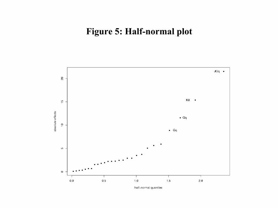
Using half-normal plots for the 27 treatment effects (Figure 5), we find that four effects

viz. JGq, k0, Qq and Gq stand apart from the rest. Using Lenth’s method (Wu and Hamada

2000, Chapter 4) as a formal test of significance, it is seen that these 4 effects are significant

at 1% level. Note that for any three-level factor X, we denote the linear and quadratic effects

(orthogonal to each other) by Xl and Xq respectively (Wu and Hamada 2000, Chapter 5).

We notice that neither the main effect of kI nor the B×kI interaction (which is estimable)

are significant. Another factor that is suspected to interact with kI is C, and we explore

the possibility of incorporating the C × kI interaction into our analysis by replacing some

insignificant effects in the preliminary model. Using the table of interactions for the L32 OA,

we find that the C × kI interaction can be estimated from columns 8 and 9 of the OA. Out

of these two columns, 8 corresponds to factor M which is seen to be insignificant and 9 is

a free column to which no other main effect or significant interaction is assigned. Thus we

14

re-perform the analysis by including the C × kI interaction (with two degrees of freedom)

instead of M .

The half-normal plot (Figure 6) now identifies 6 effects standing above the rest. Apart

from the four that were already seen to be significant, the interaction effects CkIland CkIq

turn out to be significant at 1% level.

From the plots of significant main effects (Figure 7) and the G × J interaction (Figure

8), we choose the optimal settings of k0, J , G and Q as k0 = −1,J = 1,G = 1 and Q = 2.

Note that all of these factors (or interactions involving them) were found significant in the

original analysis and the same levels (although different notations were used) were selected

as the optimum ones.

The interaction plot of C × kI (Figure 8) suggests that at neither of the two levels of C,

the optimum kI could be reached. Corresponding to C = 1, k∗I (C) ≤ 0 while corresponding

to C = −1, k∗I (C) ≥ 2. We also note that curve corresponding to C = 1 is slightly convex

as expected, whereas that corresponding to C = −1 exhibits a slight concavity, which can

be attributed to sampling error or effect of higher order interactions. Since this difference

in convexity results in significance of the quadratic component of the interaction, we may

only consider the linear component of the interaction while modelling ln ˆPM . From the

interaction plot, we choose C = −1 and kI = 2 as the optimal settings.

The following model is thus obtained:

ln PM = −5.744 + 1.241xk0 − 0.832xG + 0.334x2G + 1.073xQ − 0.586x2

Q

+0.236xCxkI− 0.124xJx2

G. (17)

Substituting the optimal settings of the control factors in the above model, we get the

optimal value of the performance measure as ln PM∗ = −8.279, which corresponds to a

standard deviation of 0.016. The original experiment was able to reduce the output stan-

dard deviation drastically to 0.031 from the existing value of 0.121. We find from this

re-analysis that with the newly recommended settings, it might have been possible to reduce

the variation to almost 50% of what had been achieved.

This analysis also points out the importance of adopting a sequential approach for the

15

performance modelling experiment. It is clear that with wider choices of levels of kI , it might

have been possible to reduce the output variance even further.

7 Concluding remarks

In this article we have developed a framework for robust parameter design of systems with

feedback control. The suggested approach can be used to obtain the optimal control law

and robust parameter design solution in a single stage. Appropriate performance measures

are developed and the design and analysis of experiments for estimation and optimization of

these performance measures are discussed. The benefits of using the proposed method are

demonstrated using an example from a packing plant.

Although we have considered the pure-gain dynamic model and primarily the discrete PI

control scheme, it should be possible to extend the proposed methodology to a much more

generic class of models and other control schemes without much difficulty. However, systems

that have on-line measurable noise factors along with provision for feedback control would

be of interest and future research may consider robust parameter design with a combination

of feedback and feedforward control.

ACKNOWLEDGEMENTS

This research was supported by the National Science Foundation (NSF) grants DMS-03-

05996 and DMI-0217395.

REFERENCES

Astrom, K.J. (1970), Introduction to Stochastic Control Theory, New York: Academic

Press.

Box, G.E.P, Jenkins G.M., and Reinsel G.C. (1994), Time Series Analysis - Forecasting

and Control, New Jersey: Prentice Hall.

16

Box, G.E.P. and Kramer, T. (1992),”Statistical Process Monitoring and Feedback Ad-

justment - A Discussion” (with discussion), Technometrics, 34, 251-285.

Box, G.E.P. and Luceno, A. (1997), Statistical Control by Monitoring and Feedback Ad-

justments, New York: Wiley.

Dasgupta, T., Sarkar, N.R., and Tamankar, K.G.T. (2002), “Using Taguchi methods to

improve a control scheme by adjustment of changeable settings”, Total Quality Management,

13, 863-876.

Davis, M.H.A., and Vinter, R.B. (1985), “Stochastic Modeling and Control”, London:

Chapman and Hall.

Del Castillo, E., and Hurwitz, A.M. (1997), “Run-to-Run Process Control: Literature

Review and Extensions,” Journal of Quality Technology, 29, 184-196.

Grove,D.M. and Davis, T.P.,“Taguchi’s Idle Column Method” (1991), Technometrics, 33,

349-353.

Huwang,L., Wu, C. F. J. and Yen, C. H.(2002), “The idle column method: construction,

properties and comparisons”, Technometrics, 44, 347-355.

Joseph, V.R. (2003), “Robust Parameter Design With Feed-Forward Control”, Techno-

metrics, 45, 284-291.

Taguchi, G. (1987), System of Experimental Design - Engineering Methods to Optimize

Quality and Minimize Costs, UNIPUB, Kraus International Publications.

Tsung, F, Wu, H, and Nair, V. N. (1998), “On the Efficiency and Robustness of Discrete

17

Proportional-Integral Control Schemes”, Technometrics, 40, 214-222.

Tsung, F, Wu, H, and Nair, V. N. (1996), “Efficiency and Robustness of Discrete

Proportional-Integral Control Schemes”, Technical Report 272, University of Michigan, Dept.

of Statistics.

Wu, C.F.J., and Hamada, M. (2000), Experiments: Planning, Analysis, and Parameter

Design Optimization, New York: Wiley.

18

Table 1: Factors and Levels, Packing Plant Experiment

Level

Control Factor 1 2 3

A. Sample frequency 10 20 −B. Sample number 3 5 −C. Sample frequency timer 240 300 −E. Main feed blanking timer (sec) 0.5 0.9 −F. Dribble feed blanking timer (sec) 0.5 0.9 −G. Discharge timer (sec) 0.3 0.6 0.9

H. Dribble feed time correction constant (sec) 0.1 0.8 −I. Gate allowance timer (sec) 0.4 2.0 −J. Feed delay timer (sec) 0.3 0.7 −L. Dribble feed quantity (start) (Kg) 8 12 −M. Discharge cut-off value (Kg) 20 30 −N. Overweight tolerance (Kg) 0.15 0.20 −P. Underweight tolerance (Kg) 0.10 0.15 −Q. Dribble feed time (sec) 1.2 1.4 1.6

Level

PI control scheme parameters 1 2 3

kI . Auto compensation proportional constant 0.2 0.3 0.4

k0. In-flight material compensation (start) 2.0 3.0 −Level

Noise factors 1 2 3

Z. Composition of material Z1 Z2 Z3

19

Table 2: Data, Packing Experiment

Variation over

Control Factor PI 3 noise levels

A B C E F G H I J L M N P Q kI k0 s.d. ln(s2)

+ − + + + 0 − + − + + − + 0 1 − 0.0584 -5.6821

− − − + − 0 − − − − + + − 1 0 + 0.1167 -4.2966

+ + − − + 0 + + − + − + − 0 1 + 0.1320 -4.0499

− + + − − 0 + − − − − − + 1 0 − 0.0979 -4.6484

+ + + − + 0 + − + − + − − 1 1 − 0.0287 -7.1007

− + − − − 0 + + + + + + + 0 0 + 0.0347 -6.7234

+ − − + + 0 − − + − − + + 1 1 + 0.1100 -4.4138

− − + + − 0 − + + + − − − 0 0 − 0.0289 -7.0905

− + + + − 2 − − − − + + + 0 1 − 0.0235 -7.4974

+ + − + + 2 − + − + + − − 1 0 + 0.1066 -4.4772

− − − − − 2 + − − − − − − 0 1 + 0.1065 -4.4792

+ − + − + 2 + + − + − + + 1 0 − 0.0421 -6.3351

− − + − − 2 + + + + + + − 1 1 − 0.0232 -7.5304

+ − − − + 2 + − + − + − + 0 0 + 0.1465 -3.8414

− + − + − 2 − + + + − − + 1 1 + 0.1021 -4.5632

+ + + + + 2 − − + − − + − 0 0 − 0.0206 -7.7693

+ − − − − 1 − + − − + − − 0 1 − 0.0165 -8.2079

− − + − + 1 − − − + + + + 2 2 + 0.1134 -4.3529

+ + + + − 1 + + − − − + + 0 1 + 0.0955 -4.6972

− + − + + 1 + − − + − − − 2 2 − 0.0130 -8.6886

+ + − + − 1 + − + + + − − 2 1 − 0.0187 -7.9619

− + + + + 1 + + + − + + + 0 2 + 0.0644 -5.4851

+ − + − − 1 − − + + − + + 2 1 + 0.1531 –3.7536

− − − − + 1 − + + − − − − 0 2 − 0.0255 -7.5840

− + − − + 2 − − − + + + + 0 1 − 0.0259 -7.3038

+ + + − − 2 − + − − + − − 2 2 + 0.1737 -3.5010

− − + + + 2 + − − + − − − 0 1 + 0.1190 -4.2572

+ − − + − 2 + + − − − + + 2 2 − 0.0222 -7.6150

− − − + + 2 + + + − + + − 2 1 − 0.0180 -8.0317

+ − + + − 2 + − + + + − + 0 2 + 0.1510 -3.7810

− + + − + 2 − + + − − − + 2 1 + 0.0311 -6.9418

+ + − − − 2 − − + + − + − 0 2 − 0.0178 -8.0519

20

Figure 1: Feedback control with control & noise factors

Process disturbanceProcess dynamicsN1, N2, ..,Nq stationary/non-stationaryfirst order / higher order

Yt = β(X,N,Ct-1 ,Ct-2 , …) + zt

X1

ProcessX2

Xp et = Yt - TCt

Control equationCt = f(et,et-1,…)

Control schemes:discrete proportional-integral (PI)minimum mean squared error (MMSE)

Figure 2: Surface plot of PM(X,kI)

0.01

0.13

0.25

0.37

0.49

0.61

0.73

0.5

1.0

1.5

21.31.41.5

1.61.7

1.8

1.9

2

2.1

2.2

2.3

PM

kI

X

Figure 3: DOE for response modelling

………………………………

Y2τ+1,..,Y3τYτ+1,..,Y2τY1,..,YτY2τ+1,..,Y3τYτ+1,..,Y2τY1,..,Yτ

X

C3C2C1C3C2C1

N2N1

et = α + g Ct-1 + zt et = α + g Ct-1 + zt

Figure 4: DOE for performance measure modeling

Yτ+1,..,Y2τY1,..,YτYτ+1,..,Y2τY1,..,YτYτ+1,..,Y2τY1,..,YτX

N2N1N2N1N2N1

kI = 2kI = 1kI = 0

PM(X,kI)

Figure 5: Half-normal plot

Figure 6 : Modified half-normal plot (with CXkIinteraction)

Figure 7: Main effects plots

MAIN EFFECT OF J

-6.4

-6.2

-6

-5.8

-5.6

-5.4

-5.2

-1 1

LEVEL

Avg(

V)

MAIN EFFECT OF k0

-7.5

-7

-6.5

-6

-5.5

-5

-4.5

-4

-1 1

LEVELS OF k0

MAIN EFFECT OF G

-6.6

-6.4

-6.2

-6

-5.8

-5.6

-5.4

-5.2

-5

0 1 2

LEVELS OF G

MAIN EFFECT OF Q

-6.6

-6.4

-6.2

-6

-5.8

-5.6

-5.4

-5.2

0 1 2

LEVELS OF Q

AVG

(v)

Figure 8: Interaction plots

GxJ interaction

-7

-6.5

-6

-5.5

-5

-4.5

0 1 2

Levels of G

Avg

(v) J=-1

J=1

C x kI Interaction plot

-9

-8

-7

-6

-5

-4

-3

0 1 2

Levels of kI

Avg

(v) C=-1

C=+1