Progress In Electromagnetics Research B, Vol. 18, 347–363, 2009 ROBUST SEMI-DETERMINISTIC FACET MODEL FOR FAST ESTIMATION ON EM SCATTERING FROM OCEAN-LIKE SURFACE H. Chen, M. Zhang, and D. Nie School of Science Xidian University Xi’an 710071, China H.-C. Yin National Electromagnetic Scattering Laboratory Beijing 100854, China Abstract—A robust semi-deterministic facet model for the computa- tion of the radar scattering cross section from the ocean-like surface is presented. As a facet-based theory, it is a more comprehensive model which can reflect the specular and diffuse configurations, as well as the mono- and bistatic features. Significant computational efficiency and good agreement with experimental data are observed, which makes the proposed facet model well suitable for fast estimation on EM scatter- ing and synthetic aperture radar (SAR) imagery simulation of marine scene. 1. INTRODUCTION Monographic study on microwave remote sensing of the ocean is an old but vigorous research realm. With the rapid development of satellite technology, which is employed for gathering information about the terrestrial or extraterrestrial and leads to the possibility of using spacecraft in remote sensing of oceanographic parameters, more and more applications to monitor ocean environment, especially as ocean synthetic aperture radar (SAR) [1–3], have been exploited during recent years. To implement these applications, a clear and comprehensive investigation on the physical processes between the electromagnetic waves and ocean surface is desirable. Approximate models, for instance, the two classical surface scattering theories: Corresponding author: M. Zhang ([email protected]).
Transcript
Progress In Electromagnetics Research B, Vol. 18, 347–363, 2009
ROBUST SEMI-DETERMINISTIC FACET MODEL FORFAST ESTIMATION ON EM SCATTERING FROMOCEAN-LIKE SURFACE
H. Chen, M. Zhang, and D. Nie
School of ScienceXidian UniversityXi’an 710071, China
H.-C. Yin
National Electromagnetic Scattering LaboratoryBeijing 100854, China
Abstract—A robust semi-deterministic facet model for the computa-tion of the radar scattering cross section from the ocean-like surface ispresented. As a facet-based theory, it is a more comprehensive modelwhich can reflect the specular and diffuse configurations, as well as themono- and bistatic features. Significant computational efficiency andgood agreement with experimental data are observed, which makes theproposed facet model well suitable for fast estimation on EM scatter-ing and synthetic aperture radar (SAR) imagery simulation of marinescene.
1. INTRODUCTION
Monographic study on microwave remote sensing of the ocean isan old but vigorous research realm. With the rapid developmentof satellite technology, which is employed for gathering informationabout the terrestrial or extraterrestrial and leads to the possibilityof using spacecraft in remote sensing of oceanographic parameters,more and more applications to monitor ocean environment, especiallyas ocean synthetic aperture radar (SAR) [1–3], have been exploitedduring recent years. To implement these applications, a clear andcomprehensive investigation on the physical processes between theelectromagnetic waves and ocean surface is desirable. Approximatemodels, for instance, the two classical surface scattering theories:
Kirchhoff approximation (KA) [4] and Small perturbation method(SPM) [5], and many unified theories like the two scale model(TSM) [6], small-slope approximation (SSA) [7], improved Green’sfunction method (IGFM) [8], extended boundary condition method(EBCM) [9] and integral equation method (IEM) [10], have beendiscussed with application to sea scatter modeling. Many of themethods mentioned above more or less meet the possible limitation onspecial rigorous valid conditions, Gaussian spectrum, monostatic radar,one dimensional surface or insurmountable computational complexity.
Nevertheless, the two scale theory has always been the mostpopular approach since it was introduced in 1970’s [11, 12]. Thekernel of the two scale theory is the theoretical division of the realsurface with two types of irregularities: Large waves whose radius ofcurvature is great enough for the calculation by KA, and fine rippleswhere SPM could be used in scattering simulation. Then the Braggscattering contributions of the small ripples would be tilted by thelarge scale components. One of the most common two-scale formulas isaccomplished by Fung et al. [13], and is called by the conventional TSMhere for distinction. Accordingly, they evaluate large scale tilt effectby averaging the backscattering cross section from perturbation theoryover the large scale slopes’ probability distribution. This is a statisticalapproach, which encompasses both large waves and small ripples toobtain an average of the real diffusion coefficient without a particularsea height map. Additionally, it meets two drawbacks: Firstly, it isnot properly accurate at angles of incidence where specular reflectionfrom the surface is significant (smaller than about 20◦, in which, thecomputational cost is also great because of the action of the lower limitof − cot θi in the integration); Secondly, although it gives a link budget,nothing is said about the radar cross section (RCS) fluctuation resultedby the local characteristics corresponding to the deterministic profileof a special sea surface. In fact, this local fluctuation is a useful featureand desirable in ocean SAR imaging model as the SAR raw signal is theappropriate superposition of returns from each facet [14]. This demandhas sprung the development of the so called “facet-based” approacheswhich try to break the surface into slightly rough plane facets withlocally approximation and represent it as a numerical elevation map,so that the instantaneous radar returns from individual facets could beobtained in SAR imagery simulation. Comparatively overall analysesare made on this topic. Franceschetti et al. [3, 14] presented a facetbackscattering model in which the Kirchhoff solution in physical opticsapproximation is used to compute the facet’s backscattering. But, insome cases the scattering properties of the facet are modeled by meansof the Bragg phenomena. This pattern has not been implemented in
Progress In Electromagnetics Research B, Vol. 18, 2009 349
their code. Hasselman et al. [15] introduced a EMH (electromagnetic-hydrodynamic) two-scale model which was fully developed on the basisof the standard plane surface Bragg resonance theory, and extended tothe so called “SAR two-scale model”. West et al. [16] also proposeda slightly-rough facet model which includes both the first-order andsecond-order large-scale effects (tilt and curvature). However, thebistatic configuration of sea scattering was not concerned in all of thefacet models above. Thus, a more comprehensive facet model whichwould adequately reflect the specular and diffuse configurations, as wellas the mono- and bistatic features, is in need.
In reinvestigation on the two scale composite theories for EMscattering from ocean surface, the original Bass-Fuks formulation ofthe two scale model draws our sight. They seek the scattered fieldin the form of the sum of a zero order approximation field (reflectedfrom the smooth surface) and a first order correction field in smallperturbation parameters. And an integration over an apparentlydeterministic profile is involved. This deterministic integration iswell suit for the extension to local facet frame. However, they onlygave the monostatic scattering formula with application to Gaussiandistribution seas [17, 18]. And, withal, in our opinion, their model stillhas poor performance in the specular zone.
In this paper, the authors fall to deriving the Bass-Fuks Two ScaleModel (BFTSM) to the bistatic case firstly. Moreover, as a numericalapproach, each facet is characterized locally by the correspondingsimulated slope on large scale oceanic surface generated by DoubleSuperimposition Method (DSM) [19]. The elementary radar returnsfrom each facet are computed by a blending scheme of combininggeometric optics limit of the KA (KA-GO) with Bragg componentsof BFTSM. Then, a facet-based summation formula of scatteringcoefficient is proposed by summing up returns from all the facets.The proposed model could well account the two types of scatteringprocesses and monostatic/bistatic configurations. In addition, it alsoresults significant computational efficiency as well as good accuracyconfirmed by experimental validation.
2. FACET STRUCTURE OF THE OCEAN SCENE
2.1. Large Scale Configuration
Many approaches were developed to describe the electromagneticscattering from oceanic surface. The most classical one is the twoscale model, which simplifies the sea wave as a superposition oftwo configurations: Gravity wave configuration and capillary waveconfiguration. In this case, the surface spectrum is classified by gravity
350 Chen et al.
wave spectrum and capillary wave spectrum, denoted by Wg and Wc
respectively. The large scale structure is described by the DoubleSuperimposition Model (DSM) [19], which describes the ocean wavefluctuating on a fixed point by many cosine wave superimpositions asfollows:
Zij(xi, yj , t) =M∑
i=1
N∑
j=1
√2Wg(ωi, θj)∆ωi∆θj
cos(kix cos θj + kiy sin θj − ωit + εij) (1)
where ki, ωi, θi represent the wave number, circle frequency anddirection angle respectively. εij could be selected randomly between0 ∼ 2π. On deep water, ki and ωi meet the relation with ω2
i = gki.The gravity wave spectrum Wg is chosen by JONSWAP spectrum asfollows:
Wg(ω, ϕ) = ϕ(ω, ϕ)αg2 1ω5
exp[−5
4
(ωm
ω
)4]· γexp
[− (ω−ωm)2
2σ2ω2m
]
(2)
ϕ(ω, ϕ) is the spreading function proposed by Stereo Wave ObservationProject:
ϕ(ω, φ) = (1 + p cos 2φ + q cos 4φ) /π, |θ| ≤ π/2 (3)
p = 0.50 + 0.82 exp[−0.5(ω/ωm)4], q = 0.32exp[−0.5(ω/ωm)4], γ is thepeak enhancement factor, σ is the peak width parameter, ωm is thefrequency of the spectral peak, ωm = 22gx−0.33/u, x = gx/U2 (x isthe wind fetch, U is the wind speed at 10 m above the mean sea level).
The large scale slope distribution of rough sea profile plays animportant role on oceanic microwave scattering calculations. Inmany of the surface scattering theories available, the probabilitydensity distribution of sea slope is described as Gaussian or Weibulldistribution. However, based on the observation data, Cox and Munkstated that the distribution of sea slope owns non-Gaussian features.They presented the probability density function of large-scale sea slopedistribution function, so called Cox-Munk PDF [20].
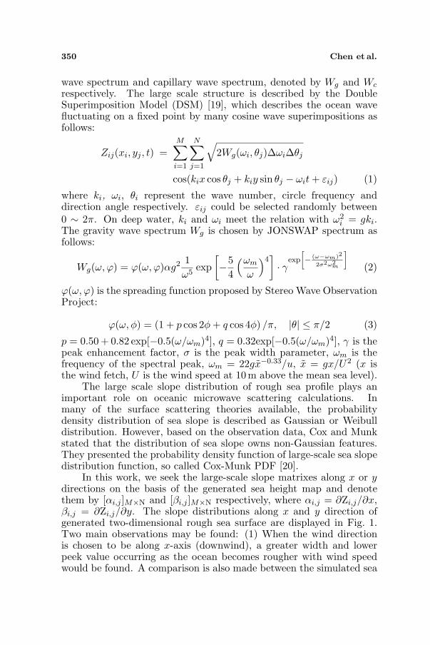
In this work, we seek the large-scale slope matrixes along x or ydirections on the basis of the generated sea height map and denotethem by [αi,j ]M×N and [βi,j ]M×N respectively, where αi,j = ∂Zi,j/∂x,βi,j = ∂Zi,j/∂y. The slope distributions along x and y direction ofgenerated two-dimensional rough sea surface are displayed in Fig. 1.Two main observations may be found: (1) When the wind directionis chosen to be along x-axis (downwind), a greater width and lowerpeek value occurring as the ocean becomes rougher with wind speedwould be found. A comparison is also made between the simulated sea
Progress In Electromagnetics Research B, Vol. 18, 2009 351
slope PDF and Cox-Munk PDF. It shows that they are comparativelyconsistent with each other (see in Figs. 1(a) and (b) in detail). Thedifference between the PDF and computational result becomes largerin Fig. 1(b). This slight inconsistency may be caused by the linearsuperimposition simplification of the sea waves as described in DSM.The slopes along x-direction could be reflected sufficiently when thedown wind blows along x-axis. While in y-direction, equivalently tocross wind, the simulated wave develops insufficiently. A non-linearprocess of the wave interaction should be introduced to improve thisissue. However, due to the simulation efficiency, this is not concernedhere. (2) When the wind speed is fixed at 5 m/s, the variations withthe wind direction is investigated in Figs. 1(c) and (d). Since thewind direction is chosen to be along the x-axis (downwind), the seasurface has more roughness along x-direction than along y-direction.Hence this leads to the narrower width and higher peak of curves alongy-direction than along x-direction. While in crosswind direction, itreverses. (Also see in Figs. 1(c) and (d)) The logical results aboveindicate that the mentioned numerical method used to simulate the
-0.6 -0.4 -0.2 0.0 0.2 0.4 0.60.000
0.002
0.004
0.006
0.008
0.010
0.012
0.014
0.016
0.018
Slo
pe d
istr
ibution a
long X
direction
Slope along X direction
0.000
0.002
0.004
0.006
0.008
0.010
0.012
0.014
0.016
(a) (b)
-0.4 -0.3 -0.2 -0.1 0.0 0.2 0.3 0.4
0.000
0.002
0.004
0.006
0.008
0.010
0.012
0.014
0.016
0.018
0.020
0.1
(c) (d)
0.000
0.002
0.004
0.006
0.008
0.010
0.012
0.014
0.016
0.018
0.020
-0.6 -0.4 -0.2 0.0 0.2 0.4 0.6Slope along Y direction
The small surface is described by the capillary spectrum Wc(K), andadapted to the real surface by a tilting process with large scale slopes.We chose the Wc(K) as the Pierson’s capillary spectrum:
Wc(K, ϕ) = Wc(k)S(k, ϕ) (4)
where
S(k, ϕ) = a0 + a1
(1− e−bk2
)cos 2ϕ
Wc(k) = 0.875·(2π)p−1 ·(1+3k2/k2
m
)g(1−p)/2
[k
(1+k2
/k2
m
)]−(p+1)/2
Detail information for each parameter above could be found in Ref. [13].
3. FACET SCATTERING MODEL
3.1. Bistatic Investigation on Bass-fuks Two Scale Model(BFTSM)
The interest in bistatic radar application has rapidly increased inrecent years. Bistatic radar can offer extra information which is notavailable from the monostatic case because of the different two-wayobservation geometry. For instance, for objects that show a low RCS inmonostatic directions, one can find suitable bistatic angles to increasetheir RCS to make them visible in radar sensing. It is worth topoint out that, oceanographic bistatic applications, especially for oceanbistiatc SAR [21, 22], is one of the most important application fields.Theoretical treatment is made on an assumed two scale model, that
0p
p
n
ˆ
ˆ
q
q
( , )i jzS
i s
x
y
z
oα
β
θ θ
sϕ
→
→
→
→
⊥
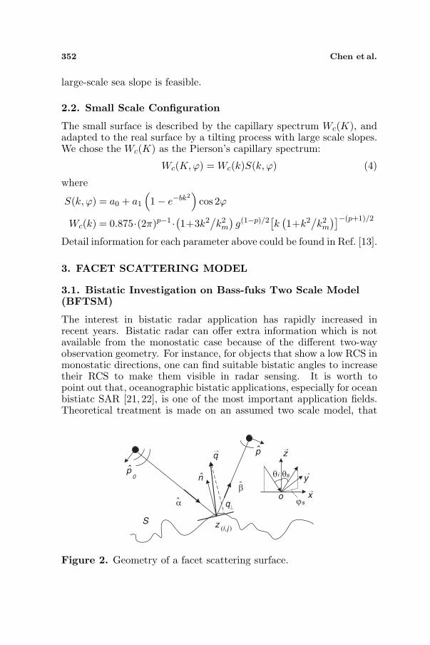
Figure 2. Geometry of a facet scattering surface.
Progress In Electromagnetics Research B, Vol. 18, 2009 353
is, treating the scattering sea surface as a combination of corrugationsof two different scales. The problem is discussed on the Geometry ofthe scattering surface shown in Fig. 2. According to the two scalescattering model presented by Bass and Fuks [12, 17, 18], we get thescattering field in case of a dielectric rough surface and a plane incidentwave.
~Es =k2eikRs
πRs
~E0
∫
S
F(p0, p, α, β, n
)ζ (~r) η
(~r, α, β
)e−i~q·~rd~r (5)
Wherein most of symbols are defined under Fig. 2, p0, p arethe unit polarization vector; α is a unit vector directed from thetransmitter, while β is a unit vector directed to the reception point;~q = k(β − α), and ε indicates the permittivity of the dielectricsurface; n points in the normal direction to the surface S, that is,n = −Zxx− Zyy + z/
√1 + Z2
x + Z2y , Zx, Zy are the large scale slopes
of each facet; η(~r, α, β) is for the possible shadowing of the surfaceS and may have two values 1 and 0 depending on whether the pointr ∈ S is illuminated or not. The function F (p0, p, α, β, n) depends onthe incident and scattering angle, different for the two polarizations,as well as the local normal unit of each facet; its detailed expression isderived in the Appendix A.
3.2. Slope-deterministic Facet Model (SDFM)
In the following context, we are only concerned with the surfacecontribution, while neglecting the multiple scattering totally. Asa numerical method, the large-scale sea surface can be fit intoapproximately by sufficient small plane facets, centered on the gridpoints. Accordingly, some facets may be in a specular configuration,while others in a diffuse configuration. The scattering coefficient bynear-specular facets can be computed under the geometric optics limitof the Kirchhoff approximation (KA-GO) [5]:
σKA = πk2q2 |Up0p|2 Prob/q4z (6)
where Prob is the Cox-Munk PDF [20]. Up0p is polarization-dependentcoefficients [5].
Since the scattering field in the bistatic formula of BFTSM isobtained in Eq. (5), in case of a plane incident wave, we can get:
σTSM =4πR2 〈EsE∗s 〉/A=8k4σ2
⟨Fp0pF
∗p0p
⟩W (q⊥, ϕ) S(θi, θs)/A (7)
where σ2 is the height variance of the small scale at resonant scatteringwave number; q⊥ is the projection of the vector ~q (~q = k(β− α)) on to
354 Chen et al.
the plane tangent at the point ~r (r ∈ S), and it is given by q⊥ =
|~q|√
1− (n · ~q/|~q|)2; W (kx, ky) is the two dimensional normalizedocean wave spectrum density and it is expressed in term of the capillaryspectrum by σ2W (K, ϕ) = Wc(K,ϕ)/K [6], Wc(K, ϕ) is defined byEq. (4). Thus, Eq. (7) can be rewritten by
σTSM = 8k4S(θi, θs)⟨Fp0pF
∗p0p
⟩Wc(Kl, ϕ)/Kl/A (8)
where Kl (Kl = q⊥) is the water wave number for resonant scattering.S(θi, θs) is employed to evaluate the shadowing effect, which isdiscussed by Bourlier et al. [23] in detail. Therefore, from Eq. (8),it could be concluded that, the returns from different facets areproportional to the instantaneous Bragg Fourier components of thecapillary spectrum, which leads to statistically independence.
Due to filter out the roughness components (some facets) forwhich the small perturbation method is inadequate, we ignore the wavenumber contribution by setting Eq. (8) to zero for Kl lower than thecut-off wave number kd. It remains no unified guideline for the selectionof the cutoff wave number kd. Different authors make different choices,which range from Johnson et al. [24] kd = k/2; Brown [25] kd = k/3;Durden and Vesecky [26] kd = k/5; Jackson et al. [27] kd = k/3 tokd = k/6; Donelan and Pierson [28] kd = k/40. A strong analysisis made by Hasselmann et al. [15]. They stated that the separationwave number kd should be at least an order of magnitude smaller thanthe incident wave number. In order to satisfy the requirements of GOfor the long-wave reflection field and the Bragg scattering theory, theyrestricted the kd by 0.05k cos θi ¿ kd ¿ k sin θi, where θi denotesthe incident angle. In this regime, the dependence of the results onthe choice of kd is weak, so that the choice kd = k/5 was applied intheir model. Soriano et al. [29] claimed that the dependence on thechoice of kd could be eliminated if the SPM is replaced by the first-order SSA in the two-scale combination. The influence of kd on theBFTSM responsible for the Bragg scattering is discussed in Fig. 3.As one can see, at smaller cutoffs, the BFTSM term dominates morein the specular angles (smaller than 20◦). Here, we choose kd = k/4empirically.
It has clear physical grounds to revise the TSM by a combinationof KA with TSM contributions, rather than adding KA to SPM [26, 30].Andreas et al. [30] released a “semi-deterministic” frame under whichthe facet context is locally characterized by the so-called “bistatic localangles” at a deterministic surface profile. They restrict the specularreflection zone with the local specular angles approximately below 20◦,and introduce a weight factor to smooth the transition between thespecular and diffuse region. Although the factor needs a theoretical
Progress In Electromagnetics Research B, Vol. 18, 2009 355
treatment of a more clear explain. Accordingly, we present a facet-based summation formula in which the elementary radar returns fromrespective facets are computed by the semi-deterministic scheme ofcombining geometric optics limit of the KA (KA-GO) with Braggcomponents of the extended BFTSM. It is quite similar to the schemepresented by Andreas et al.. In contrast, however, we relate the localconfigurations mainly to the sea slopes of the large scale profile andthe Bragg-scattering part of the wave number spectrum. The implicitweight factor which is relevant to smooth the break point result by theregion transition and the “local angle” division are not used. In orderto apply the facet Bragg theory, the facet must be large in comparisonwith the wavelength of the incident radiation in the facet plane, andbe sufficiently small as it can still be regarded as a plane [15]. Wepostulate the discrete facets are in proper size, so that the KA andTSM can be used in the local summation frame. In our treatment, thesurface is generated by 300× 300 facets, and the respective resolutionhas been considered as 1×1 meters. This is a statistical approach, and,experimentally, in the semi-deterministic diagram, the RCS averagedoes not depend much upon the facet size [30]. Then, under a “semi-deterministic” scheme, the total scattering coefficient can be obtainedby summing up returns from all the Bragg facets, including the non-Bragg contributions governed by Eq. (6):
σp0p∑ =S(θi, θs)
A
M∑
i=1
N∑
j=1
[8k4F p0p
i,j F p0p∗i,j Wc(Kl, ϕ)/Kl
+πk2q2∣∣∣Up0p
i,j
∣∣∣2Prob/q4
z
]∣∣∣∣Zyij={Zyij∈[βij ]}
Zxij={Zxij∈[αij ]|Zxij>− cot θi}(9)
Due to avoid illuminating the rear of the tilted facets, the slopes
along the x direction are limited above − cot θi. A is the area of thegenerated sea surface.
Under the facet scheme, the monostatic average varied withincident angles is obtained as a blend of KA-GO and k/4 cutoff Braggcomponents of BFTSM (also see in Fig. 3), when the incident frequencyis set to 14.0 GHz, for VV and HH polarizations. Fig. 4 displaysthe simulated returns from individual facets in the backscatteringdirection as the incident angle equals to 40◦. Other parameters arefixed as: Wind direction: upwind; VV polarization; incident frequency:14.0GHz; wind speed: 5m/s; sea simulation plot: 300 m× 300m.
0 5 10 15 20 25 30 35 40 45 50 55Incident angle
0 5 10 15 20 25 30 35 40 45 50 55
-50
-45
-40
-35
-30
-25
-20
-15
-10
-5
0
5
10
1520
-35
-30
-25
-20
-15
-10
-5
0
5
10
15
20
Monosta
tic s
cattering c
oeffic
ient
(dB
)
(a) (b)
Monosta
tic s
cattering c
oeffic
ient
(dB
)
Incident angle
Figure 5. Experiment validation on impact of wind direction: (a) ForVV polarization; (b) for HH polarization.
Table 1. The cost time on calculating the backscattering coefficienta.
ComparisonItem
Generatedsea model
HH polarization VV polarization
CTSM No need 333.687 s 410.343 sSDFM 21.875 s 87.297 s 87.375 s
aThe calculating parameters: a) Incident angle range: 1◦ ∼ 89◦,f = 14.0Ghz; u = 6.267m/s, sea area 200× 200m2, Upwind; b)computer capacity: Inter(R) Core(TM) 2 Quad CPU 2.50 GHz
2.49GHz, 2.0GB.
Progress In Electromagnetics Research B, Vol. 18, 2009 357
4. RESULTS ANALYSIS AND EXPERIMENTALVALIDATION
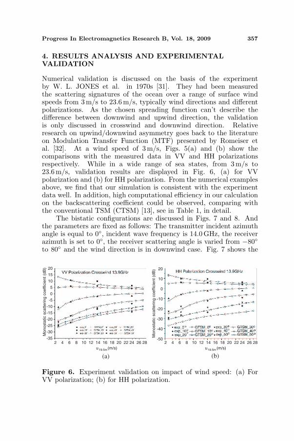
Numerical validation is discussed on the basis of the experimentby W. L. JONES et al. in 1970s [31]. They had been measuredthe scattering signatures of the ocean over a range of surface windspeeds from 3 m/s to 23.6 m/s, typically wind directions and differentpolarizations. As the chosen spreading function can’t describe thedifference between downwind and upwind direction, the validationis only discussed in crosswind and downwind direction. Relativeresearch on upwind/downwind asymmetry goes back to the literatureon Modulation Transfer Function (MTF) presented by Romeiser etal. [32]. At a wind speed of 3m/s, Figs. 5(a) and (b) show thecomparisons with the measured data in VV and HH polarizationsrespectively. While in a wide range of sea states, from 3m/s to23.6m/s, validation results are displayed in Fig. 6, (a) for VVpolarization and (b) for HH polarization. From the numerical examplesabove, we find that our simulation is consistent with the experimentdata well. In addition, high computational efficiency in our calculationon the backscattering coefficient could be observed, comparing withthe conventional TSM (CTSM) [13], see in Table 1, in detail.
The bistatic configurations are discussed in Figs. 7 and 8. Andthe parameters are fixed as follows: The transmitter incident azimuthangle is equal to 0◦, incident wave frequency is 14.0 GHz, the receiverazimuth is set to 0◦, the receiver scattering angle is varied from −80◦to 80◦ and the wind direction is in downwind case. Fig. 7 shows the
2 4 6 8 10 12 14 16 18 20 22 24 26 28-35
-30
-25
-20
-15
-10
-5
0
5
10
15
20
Mo
no
sta
tic s
ca
tte
rin
g c
oe
ffic
ien
t (d
B)
u (m/s)19.5m
2 4 6 8 10 12 14 16 18 20 22 24 26 28-50
-40
-30
-20
-10
0
10
20
(a) (b)
Mo
no
sta
tic s
ca
tte
rin
g c
oe
ffic
ien
t (d
B)
u (m/s)19.5m
Figure 6. Experiment validation on impact of wind speed: (a) ForVV polarization; (b) for HH polarization.
bistatic simulations by SDFM for two wind speeds, 5 m/s and 8 m/s,respectively, and the transmitter incident angle is 40◦. As is apparent,the maximum energy is received around the specular direction 40◦, andit decreases when the wind speed increases, which is a logical result.Fig. 8 compares the results yielded by the first order SSA [33] withSDFM for 5 m/s in HH and VV polarizations respectively, while thetransmitter incident angle is 50◦. It shows good agreement betweenSSA and SDFM, as the difference remains within about 2 dB.
5. CONCLUSION
A slope-deterministic facet model for the computation of the radarscattering cross section from the ocean-like surface is presented. As anumerical theory, it is a more comprehensive facet model which canreflect the specular and diffuse configurations, as well as the mono-and bistatic configurations. Combining all of these features under thefacet-based frame may be outlined for the first time. Finally, the goodagreement between the model results and available experimental dataencourages us to employ the proposed model for further investigationson bistatic realistic SAR imagery simulations of marine scene.
ACKNOWLEDGMENT
The authors thank the National Nature Science Foundation of Chinaunder Grant No. 60871070, the National Pre-research Foundation andthe Foundation of the National Electromagnetic Scattering Laboratoryfor supporting this research.
Progress In Electromagnetics Research B, Vol. 18, 2009 359
APPENDIX A.
As defined under the geometry in Fig. 2, the related parameters canbe denoted as follows:
α = sin θi cosϕix + sin θi sinϕiy − cos θiz
β = sin θs cosϕsx + sin θs sinϕsy + cos θsz
p0h = − sinϕix + cosϕiy
p0v = − cos θi cosϕix− cos θi sinϕiy − sin θiz
ph = − sinϕsx + cos ϕsy
pv = cos θs cosϕsx + cos θs sinϕsy − sin θsz
Then, the function F (p0, p, α, β, n) can be expressed as:
Avv =cos θi cosϕi cos θs cosϕs+cos θi sinϕi cos θs sinϕs−sin θi sin θs
Bvv =−d2 (Zx cos θi cosϕi + Zy cos θi sinϕi − sin θi)× (−Zx cos θs cosϕs − Zy cos θs sinϕs − sin θs)Cvv =−d (−Zx cos θs cosϕs − Zy cos θs sinϕs − sin θs)× (− cos θi cosϕi sin θs cosϕs − cos θi sinϕi sin θs sinϕs − sin θi cos θs)Dvv =−d (Zx cos θi cosϕi + Zy cos θi sinϕi − sin θi)× (sin θi cosϕi cos θs cosϕs + sin θi sinϕi cos θs sinϕs + cos θi sin θs)Qvv =−Bvv (sin θi cosϕi sin θs cosϕs+sin θi sinϕi sin θs sinϕs
− cos θi cos θs)+a (sin θi cosϕi cos θs cosϕs + sin θi sinϕi cos θs sinϕs
hh=−Bhh(sin θi cosϕi sin θs cosϕs+sin θi sinϕi sin θs sinϕs
− cos θi cos θs) + a(sin θi sinϕi cosϕs−sin θi cosϕi sinϕs)
Similarly, the parameters above can be obtained for crosspolarizations.
REFERENCES
1. Franceschetti, G., M. Migliaccio, and D. Riccio, “On oceanSAR raw signal simulation,” IEEE Trans. Geosci. Remote Sens.,Vol. 36, No. 1, 84–100, 1998.
2. Kasilingram, D. P. and O. H. Shemdin, “Models for syntheticaperture radar imaging of the ocean: A comparison,” J. Geophys.Res., Vol. 95, 16263–16276, 1990.
3. Franceschetti, G., A. Iodice, D. Riccio, G. Ruello, and R. Siviero,“SAR raw signal simulation of oil slicks in ocean environments,”IEEE Trans. Geosci. Remote Sens., Vol. 40, No. 9, 1935–1949,2002.
4. Beckmann, P. and A. Spizzichino, The Scattering of Electromag-netic Waves from Rough Surfaces, Macmillan, New York, 1963.
5. Ulaby, F. T., R. K. Moore, and A. K. Fung, Microwave RemoteSensing: Active and Passive, Vol. 2, Artech House, Norwood, MA,1986.
6. Chan, H. L. and A. K. Fung, “A theory of sea scatter at largeincident angles,” J. Geophys. Res., Vol. 82, 3439–3444, 1977.
Progress In Electromagnetics Research B, Vol. 18, 2009 361
7. Voronovich, A. G., “Small-slope approximation for electromag-netic wave scattering at a rough interface of two dielectric half-spaces,” Waves Random Media, Vol. 4, 337–367, 1994.
8. Shaw, W. T. and A. J. Dougan, “Green’s function refinement as anapproach to radar backscatter: General theory and application toLGA scattering form the ocean,” IEEE Trans. Antennas Propag.,Vol. 46, 57–66, 1998.
9. Guo, L. and Z. Wu, “Application of the extended boundarycondition method to electromagnetic scattering from roughdielectric fractal sea surface,” Journal of Electromagnetic Wavesand Applications, Vol. 18, No. 9, 1219–1234, 2004.
10. Nedlin, G. M., S. R. Chubb, and A. L. Cooper, “The integralequation method for electromagnetic scattering from the ocean:Beyond a perfect conductor model,” Radio Sci., Vol. 34, No. 1,27–49, 1999.
11. Valenzuela, G. R., “Theories for the interaction of electromagneticwaves and oceanic waves: A review,” Bound. Layer Met., Vol. 13,61–85, 1978.
12. Bass, F. G. and I. M. Fuks, Wave Scattering from StatisticallyRough Surfaces, 418–442, Pergamon Press Oxford, New York,1979.
13. Fung, A. K. and K. Lee, “A semi-empirical sea-spectrum model forscattering coefficient estimation,” IEEE J. Oceanic Engineering,Vol. 7, No. 4, 166–176, 1982.
14. Franceschetti, G., M. Migliaccio, D. Riccio, and G. Schirinzi,“SARAS: A synthetic aperture radar (SAR) raw signal simulator,”IEEE Trans. Geosci. Remote Sens., Vol. 30, No. 1, 110–123, 1992.
15. Hasselman, K., et al., “Theory of synthetic aperture radar oceanimaging: A MARSEN view,” J. Geophys. Res., Vol. 90, 4659–4686, 1985.
16. West, J. C., R. K. Moore, and J. C. Holtzman, “The slightly-rough facet model in radar imaging of the ocean surface,” Int. J.Remote Sens., Vol. 11, No. 4, 617–637, 1990.
17. Fuks, I. M., “Theory of radio wave scattering at a rough seasurface,” Radiophysics and Quantum Electronics, Vol. 9, No. 5,513–519, 1966.
18. Bass, F. G., I. M. Fuks, et al., “Very high frequency radiowavescattering by a disturbed sea surface,” IEEE Trans. AntennasPropagat., Vol. 16, No. 5, 554–568, 1968.
19. Joung, S. and J. Shelton, “3 Dimensional ocean wave modelusing directional wave spectra for limited capacity computers,”
362 Chen et al.
IEEE OCEANS ‘91.’ Ocean Technologies and Opportunities inthe Pacific for the 90‘s’. Proceedings., Vol. 1, 608–614, 1991.
20. Cox, C. and W. H. Munk, “Statistics of the sea surface derivedfrom sun glitter,” J. Marine Res., Vol. 13, 198–227, 1954.
21. Moccia, A., G. Rufino, and M. D. Luca, “Oceanographic applica-tions of spaceborne bistatic SAR,” IEEE International Geoscienceand Remote Sensing Symposium, IGARSS’03. Proceedings., Vol. 3No. 21–25, 1452–1454, 2003.
22. Kassem, M. J. B., J. Saillard, and A. Khenchaf, “BISAR mappingI. Theory and modelling,” Progress In Electromagnetics Research,PIER 61, 39–65, 2006.
23. Bourlier, C., G. Berginc, and J. Saillard, “One and two-dimensional stationary shadowing functions for any height andslope stationary uncorrelated surface in the monostatic andbistatic configureations,” IEEE Trans. Antennas Propagat.,Vol. 50, No. 3, 312–324, 2002.
24. Johnson, J. T., R. T. Shinan, and J. A. Kong, “A numerical studyof the composite surface model for ocean backscattering,” IEEETrans. Geosci. Remote Sens., Vol. 36, 72–83, 1998.
25. Brown, G. S., “Backscattering from a Gaussian-distributed,perfectly conducting rough surface,” IEEE Trans. AntennasPropag., Vol. 26, 472–482, 1978.
26. Durden, S. L. and J. F. Vesecky, “A physical radar cross-section model for a wind-driven sea with swell,” IEEE J. OceanicEngineering, Vol. 10, 445–451, 1985.
27. Jackson, F. C., W. T. Walton, and D. E. Hines, “Sea surface meansquare slope from Ku-band backscatter data,” J. Geophys. Res.,Vol. 11, 411–427, 1997.
28. Donelan, M. A. and W. J. Pierson, “Radar scattering andequilibrium ranges in wind-generated waves with application toscatterometry,” J. Geophys. Res., Vol. 92, 4971–5029, 1987.
29. Soriano, G. and C. A. Guerin, “A cutoff invariant two-scale modelin electromagnetic scattering from sea surfaces,” IEEE Trans.Geosci. Remote Sens., Vol. 5, 199–203, 2008.
30. Andreas, A. B., A. Khenchaf, and A. Martin, “Bistaticradar imaging of the marine environment Part I: Theoreticalbackground,” IEEE Trans. Geosci. Remote Sens., Vol. 45, No. 11,3372–3383, 2007.
31. Jones, W. L., L. C. Schroeder, and J. L. Mitchell, “Aircraftmeasurements of the microwave scattering signature of the ocean,”IEEE Trans. Antennas Propagat., Vol. 25, No. 1, 52–61, 1977.
Progress In Electromagnetics Research B, Vol. 18, 2009 363
32. Romeiser, R., W. Alpers, and V. Wismann, “An improvedcomposite surface model for the radar backscattering crosssection of the ocean surface 1. Theory of the model andoptimization/validation by scatterometer data,” J. Geophys. Res.,Vol. 102, 25237–25250, 1997.
33. Awada, A., M. Y. Ayari, A. Khenchaf, and A. Coatanhay,“Bistatic scattering from an anisotropic sea surface: Numericalcomparison between the first-order SSA and the TSM models,”Waves in Random and Complex Media, Vol. 16, No. 3, 383–394,2006.