Robust Surface Reconstruction via Triple Sparsity Hicham Badri INRIA, Geostat team 33400 Talence, France [email protected]Hussein Yahia INRIA, Geostat team 33400 Talence, France [email protected]Driss Aboutajdine LRIT - CNRST (URAC29) 1014 RP Rabat, Morocco [email protected]Abstract Reconstructing a surface/image from corrupted gradient fields is a crucial step in many imaging applications where a gradient field is subject to both noise and unlocalized outliers, resulting typically in a non-integrable field. We present in this paper a new optimization method for robust surface reconstruction. The proposed formulation is based on a triple sparsity prior : a sparse prior on the residual gradient field and a double sparse prior on the surface gra- dients. We develop an efficient alternate minimization strat- egy to solve the proposed optimization problem. The method is able to recover a good quality surface from severely cor- rupted gradients thanks to its ability to handle both noise and outliers. We demonstrate the performance of the pro- posed method on synthetic and real data. Experiments show that the proposed solution outperforms some existing meth- ods in the three possible cases : noise only, outliers only and mixed noise/outliers. 1. Introduction Reconstruction from corrupted gradient fields is a task of primary importance in several imaging applications. For in- stance, recovering the surface shape from captured images using Photometric Stereo (PS) [17] and Shape from Shad- ing (SFS) [8] requires robust surface reconstruction tools to integrate surface normal vectors. Many computational pho- tography applications such as HDR compression [5], image editing [12], stitching [10], super-resolution [16], manipu- late image gradients and reconstruct a new image from the resulting gradient field. Integration is also used to recover an image from its incomplete Fourier measurements after estimating the corresponding gradients using Compressed Sensing methods [11]. In all the applications above, the resulting gradient field is non-integrable either due to er- rors in measurements including noise and/or outliers, or the corresponding gradient field is directly modified by mixing multiple gradients of different images, or simply applying linear/nonlinear functions. This paper proposes a new opti- mization method for robust surface reconstruction from cor- rupted gradient fields. Unlike previous optimization formu- lations [15, 14, 4, 2, 7], we consider a triple sparsity prior : a double sparse prior, on the gradient residual and the surface gradients, aims at efficiently handling gradient field outliers. A third sparse prior improves reconstruction quality in the case of gradient noise. The contributions are as follows : • We present a new optimization method for robust re- construction of sparse gradient signals from corrupted gradient fields, handling both noise and outliers. • We propose an efficient alternate minimization strat- egy to solve the proposed problem. • We demonstrate the performance of the proposed framework on synthetic and real data and compare it to some existing reconstruction methods. 2. Related Work Enforcing integrability can be traced back to the work of Chellappa et al. [15, 6] for problems such as Shape from Shading. Poisson reconstruction [6] is probably the most popular approach to integration. It consists in solv- ing the Poisson equation that is derived from a straightfor- ward least-squares fit. It is well known that least squares solutions are not robust to outliers [14]. What happens in the problem of integration is that, when using a least squares solution, the errors are propagated and can result in an unnatural surface/image even if only few gradient points are corrupted as can be seen in Figure 1. The Frankot- Chellappa method [15] performs a projection of the non- integrable gradient field in the Fourier basis. The technique was extended to non-orthogonal set of basis functions such as shapelets [9]. Petrovic et al. [13] propose a loopy be- lief propagation integration method when the gradient field is corrupted with a Gaussian noise. Agrawal et al. pro- pose in [2] a more general framework to extend the Poisson equation. Another method by Agrawal et al. consists in cor- recting the gradient field with an algebraic method [1]. The method produces impressive results when the gradient field
Reconstructing a surface/image from corrupted gradientfields is a crucial step in many imaging applications wherea gradient field is subject to both noise and unlocalizedoutliers, resulting typically in a non-integrable field. Wepresent in this paper a new optimization method for robustsurface reconstruction. The proposed formulation is basedon a triple sparsity prior : a sparse prior on the residualgradient field and a double sparse prior on the surface gra-dients. We develop an efficient alternate minimization strat-egy to solve the proposed optimization problem. The methodis able to recover a good quality surface from severely cor-rupted gradients thanks to its ability to handle both noiseand outliers. We demonstrate the performance of the pro-posed method on synthetic and real data. Experiments showthat the proposed solution outperforms some existing meth-ods in the three possible cases : noise only, outliers onlyand mixed noise/outliers.
1. IntroductionReconstruction from corrupted gradient fields is a task of
primary importance in several imaging applications. For in-stance, recovering the surface shape from captured imagesusing Photometric Stereo (PS) [17] and Shape from Shad-ing (SFS) [8] requires robust surface reconstruction tools tointegrate surface normal vectors. Many computational pho-tography applications such as HDR compression [5], imageediting [12], stitching [10], super-resolution [16], manipu-late image gradients and reconstruct a new image from theresulting gradient field. Integration is also used to recoveran image from its incomplete Fourier measurements afterestimating the corresponding gradients using CompressedSensing methods [11]. In all the applications above, theresulting gradient field is non-integrable either due to er-rors in measurements including noise and/or outliers, or thecorresponding gradient field is directly modified by mixingmultiple gradients of different images, or simply applyinglinear/nonlinear functions. This paper proposes a new opti-
mization method for robust surface reconstruction from cor-rupted gradient fields. Unlike previous optimization formu-lations [15, 14, 4, 2, 7], we consider a triple sparsity prior : adouble sparse prior, on the gradient residual and the surfacegradients, aims at efficiently handling gradient field outliers.A third sparse prior improves reconstruction quality in thecase of gradient noise. The contributions are as follows :
• We present a new optimization method for robust re-construction of sparse gradient signals from corruptedgradient fields, handling both noise and outliers.
• We propose an efficient alternate minimization strat-egy to solve the proposed problem.
• We demonstrate the performance of the proposedframework on synthetic and real data and compare itto some existing reconstruction methods.
2. Related WorkEnforcing integrability can be traced back to the work
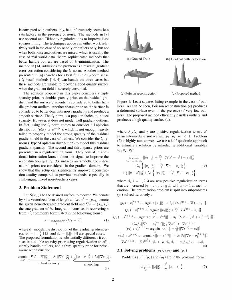
of Chellappa et al. [15, 6] for problems such as Shapefrom Shading. Poisson reconstruction [6] is probably themost popular approach to integration. It consists in solv-ing the Poisson equation that is derived from a straightfor-ward least-squares fit. It is well known that least squaressolutions are not robust to outliers [14]. What happensin the problem of integration is that, when using a leastsquares solution, the errors are propagated and can result inan unnatural surface/image even if only few gradient pointsare corrupted as can be seen in Figure 1. The Frankot-Chellappa method [15] performs a projection of the non-integrable gradient field in the Fourier basis. The techniquewas extended to non-orthogonal set of basis functions suchas shapelets [9]. Petrovic et al. [13] propose a loopy be-lief propagation integration method when the gradient fieldis corrupted with a Gaussian noise. Agrawal et al. pro-pose in [2] a more general framework to extend the Poissonequation. Another method by Agrawal et al. consists in cor-recting the gradient field with an algebraic method [1]. Themethod produces impressive results when the gradient field
is corrupted with outliers only, but unfortunately seems lesssatisfactory in the presence of noise. The methods in [7]use spectral and Tikhonov regularizations to improve leastsquares fitting. The techniques above can either work rela-tively well in the case of noise only or outliers only, but notwhen both noise and outliers are mixed, which is usually thecase of real world data. More sophisticated methods thatbetter handle outliers are based on l1-minimization. Themethod in [14] addresses the problem as a residual gradienterror correction considering the l1-norm. Another methodpresented in [4] searches for a best fit in the l1-norm sense; l1-based methods [14, 4] can handle the three cases butthese methods are unable to recover a good quality surfacewhen the gradient field is severely corrupted.
The solution proposed in this paper considers a triplesparsity prior. A double sparsity prior, on the residual gra-dient and the surface gradients, is considered to better han-dle gradient outliers. Another sparse prior on the surface isconsidered to better deal with noisy gradients and produce asmooth surface. The l1-norm is a popular choice to inducesparsity. However, it does not model well gradient outliers.In fact, using the l1-norm comes to consider a Laplaciandistribution (p(x) ∝ e−τ |x|), which is not enough heavilytailed to properly model the strong sparsity of the residualgradient field in the case of outliers. We consider the lp<1-norm (Hyper-Laplacian distribution) to model this residualgradient sparsity. The second and third sparse priors arepresented in a regularization form. They consist in addi-tional information known about the signal to improve thereconstruction quality. As surfaces are smooth, the sparsenatural priors are considered in the gradient domain. Weshow that this setup can significantly improve reconstruc-tion quality compared to previous methods, especially inchallenging mixed noise/outliers cases.
3. Problem StatementLet S(x, y) be the desired surface to recover. We denote
by s its vectorized form of length n. Let −→v = (p, q) denotethe given non-integrable gradient field and ∇s = (sx, sy)the true gradient of S. Integration consists in recovering sfrom −→v , commonly formulated in the following form :
s = argmins
φr(∇s−−→v ). (1)
where φr models the distribution of the residual gradient er-ror. φr = ||.||22 [15] and φr = ||.||1 [4] are special cases.The proposed formulation is substantially different : it con-sists in a double sparsity prior using regularization to effi-ciently handle outliers, and a third sparsity prior for noise-aware reconstruction :
Figure 1: Least squares fitting example in the case of out-liers. As can be seen, Poisson reconstruction (c) producesa deformed surface even in the presence of very few out-liers. The proposed method efficiently handles outliers andproduces a high quality surface (d).
where λ1,λ2 and γ are positive regularization terms, s′
is an intermediate surface and p1, p2, p3 < 1. Problem(2) is highly non-convex, we use a half-quadratic approachto estimate a solution by introducing additional variablesv1, v2, v3 :
argmins,s′,v1,v2,v3
||v1||p1p1 +β1
2 ||(∇s′ −−→v )− v1||22
+λ1
{||v2||p2p2 +
β2
2 ||∇s′ − v2||22
}+γ
2 ||s− s′||22 + λ2
{||v3||p3p3 +
β3
2 ||∇s− v3||22
},
(3)
where βi, i = 1, 2, 3 are new positive regularization termsthat are increased by multiplying βi with κi > 1 at each it-eration. The optimization problem is split into subproblems(pi) solved iteratively :
Problems (p1), (p2) and (p4) are in the proximal form :
argminv||v||pp +
β
2||x− v||22, (5)
2
the solution is given via generalized soft-thresholding [3] :
v = shrinklp(x, β) = max{0, |x| − |x|
p−1
β
}x
|x|. (6)
The special case of p = 0 consists in hard-thresholding [18]
v = shrinkl0(x, β) =
{0 |x|2 ≤ 2
β
x otherwise.(7)
Note however that v in our case is a 2-components vector.We adopt an anisotropic approach which consists in apply-ing the thresholding on each vector field component sepa-rately. Thus, the solutions to problems (pj), j = 1, 2 are
v(k+1)j =
v(k+1)j,x (i) = shrinklp
(∇xs′(k)(i)− vx(i), βj
)v(k+1)j,y (i) = shrinklp
(∇ys′(k)(i)− vy(i), βj
)i = 1, ..., n,
(8)and the solution to problem (p3) is given as follows :
v(k+1)3 =
v(k+1)3,x (i) = shrinklp
(∇xs(k)(i), β3
)v(k+1)3,y (i) = shrinklp
(∇ys(k)(i), β3
)i = 1, ..., n.
(9)
3.2. Solving problems (p3) and (p5)
Problem (p5) is quadratic and easy to solve via Euler-Lagrange equation. The solution can be computed either bysolving a linear system such that∇x ≈ (Dxx,Dyx), whereDx and Dy are differential operators in the matrix form, orperforming a deconvolution using the Fourier transform Fsuch that∇x ≈ (x?
[1 −1
]T, x?
[1 −1
]), where ?
is the convolution operator. Considering periodic boundaryconditions, we choose the Fourier transform method thatgives the following solution :
s(k+1) = F−1F
(γs′(k) − λ2β3div(v(k+1)
3 ))
γ − λ2β3lap
. (10)
where div is the discrete divergence operator and lap is theFourier transform of the discrete Laplacian filter. Problem(p3) is similar. By applying the Euler-Lagrange equationand considering the Fourier method, the solution to problem(p3) is given as follows :
s′(k+1) = F−1(F(γs(k)−div(u))γ−(β1+λβ2)lap
)u = β1(
−→v + v(k+1)1 ) + λβ2v
(k+1)2 .
(11)
3.3. Justification
To show why and how the proposed approach improvesthe quality of the reconstruction, we propose to study sepa-rately the robust reconstruction step which consists in solv-ing problems (p1), (p2) and (p3) in the case of strong out-liers, and then show why problems (p4) and (p5) are impor-tant in the case of noisy gradients.
3.3.1 Why Double Sparsity for Outliers?
The proposed formulation (2) is composed of two parts : adouble sparsity part for robust recovery and a sparsity priorfor smoothing. We consider in this section only the robustrecovery part (γ = 0 and λ2 = 0) to see how the proposedrecovery formulation improves reconstruction in the case ofstrong outliers. The robust reconstruction step consists insolving the following optimization problem :
argmins′||∇s′ −−→v ||p1p1 + λ1||∇s′||p2p2 . (12)
Outliers consist in sparse errors with strong magnitude (duefor instance to depth discontinuities and shadows). A leastsquares fit (p1 = 2 and λ1 = 0) tends to propagate er-rors and results in a corrupted surface as it was shown inFigure 1. The reason why this happens is that, when usingthe l2 norm, the distribution of the residual gradient error∇s′ − −→v is modeled using a Gaussian which is not appro-priate when the gradient is corrupted with outliers only. In-stead, the model should take into account the sparsity of theresidual gradient, which comes to the cost of using the lp≤1norm. However, the l1-norm does not model well either thestrong sparsity of the residual gradient, which makes the re-covery of the surface only possible when the number of out-liers is relatively low. Thus, our choice for the lp<1-normwhich models better the heavy-tailed distribution of the gra-dient errors in the case of outliers. Note that, using the lp<1
norm alone, the performance is rather limited. In fact, usingthe lp-norm on the residual gradients is a maximum likeli-hood (MP) estimation which can be improved with a MAPestimation instead. The MAP estimation in our case con-sists in regularizing the MP estimation with a natural prior.The natural prior that we choose is the smoothness of thesurface itself, hence the use of the lp-norm on the gradientof s′ too.
To properly evaluate the importance of the proposed dou-ble sparsity model, we run reconstruction experiments onthe Shepp-Logan phantom instance and study the case ofexact recovery of the image from corrupted gradients withoutliers. We use this image because it is a standard bench-mark instance for exact recovery in Compressed Sensingapplications. Note that here, we reconstruct the imagefrom corrupted gradients with outliers and not incompleteFourier measurements as the image instance is usually usedfor. Outliers are generated as sparse random errors with astrong magnitude. We study the case of l2, diffusion [2] ,l1,lp(p = 0.1) and the proposed double lp (p = 0.1 for bothp1 and p2) model and present the results in Figure 2. Ascan be seen, the proposed method is able to recover exactlythe original image even in the presence of a high level ofoutliers.
3
(a) Ground Truth (b) Least Squares [15] (c) Diffusion [2]
(d) l1 [14] (e) lp<1 fit (f) Double lp<1
Figure 2: Reconstruction quality comparison between theproposed double sparsity model and some other methods.Exact recovery is possible with the proposed method evenin the case of strong outliers (more than 12% of the gradientpoints were corrupted with random sparse high magnitudeerrors. The magnitude of the outliers is 10 times the maxi-mum of the gradient norm max
(√∇xs2 +∇ys2
)).
3.4. Why a Third Sparsity for Noise?
We saw in the previous section how the double sparsityprior improves the quality of recovery in the case of out-liers. Note however, that when solving problem (12), whichconsists in solving sub-problems (p1), (p2) and (p3), thereis no step to smooth the surface in the case of noise. Thus,using the formulation (12) for the mixed noise/outliers casecan successfully correct outliers but cannot denoise the sur-face. Hence, we introduce a denoising step which consistsin using another sparse gradient prior as follows :
argmins
γ
2||s− s′||22 + λ2||∇s||p3p3 . (13)
When problems (12) and (13) are combined, it gives prob-lem (2) which is solved iteratively by correcting the outliers(problems (p1), (p2) and (p3)) followed by a denoising step(problems (p4), (p5)). To show the importance of this thirdsparsity model compared to the previous double sparsitymodel, we run reconstruction experiments on the Shepp-Logan phantom instance and study the case of near exactrecovery of the image from corrupted gradients with noiseand outliers. We generate a random Gaussian noise and thesame amount of outliers as the previous section. Results arepresented in Figure 3. As can be seen, improved recovery isobtained with the triple sparsity model. The double sparsitymodel corrects outliers but does not get rid of the noise.
Due to the high non-convexity of the proposed optimiza-
(a) Ground Truth (b) Least Squares [15] (c) Diffusion [2]
(d) lp<1 fit (e) Double lp<1 (f) Triple lp<1
Figure 3: Reconstruction quality comparison in the case ofboth noise and outliers. The double sparsity model correctsoutliers but does not denoise the output. The third spar-sity prior permits to denoise the instance while correctingoutliers resulting in a near-exact recovery (σ = 7% of themaximum intensity value, with the same outliers level as 2).
tion problem, the half-quadratic solver cannot reach a globalminimum. However, experiments show that the methodconverges to a local minimum after a certain number of it-erations. The solver starts with a trivial solution (Poissonreconstruction) and iteratively corrects the vector field. Ifthe gradients are error-free, the trivial solution is the truesurface, which leads to a zero residual gradient error.
4. ResultsTo evaluate the proposed solution, we run multiple ex-
periments including synthetic and real data. Similar to pre-vious work, we first compare the method on the RampPeaks dataset which is a standard benchmark surface [2,14, 4]. We use the same parameters so the reader can com-pare the results with other methods that can be found in thepapers just cited. The second experiment consists in Pho-tometric Stereo on the synthetic Mozart and Vase datasetsused in [14, 2]. The third experiment consists in Photomet-ric Stereo on real noisy images.
4.1. Surface Reconstruction
We corrupt a gradient field and try to reconstruct the sur-face from the resulting non-integrable field. We use theRamp Peaks synthetic dataset considering the three cases.The MSE is reported in Table 1.
Noise only : We add Gaussian noise to the ground truthgradient field and try to recover it. We take the same pa-rameters as the previous work (σ = 10% of the maxi-
4
(a) Ground Truth (b) Least Squares [15] (c) Diffusion [2]
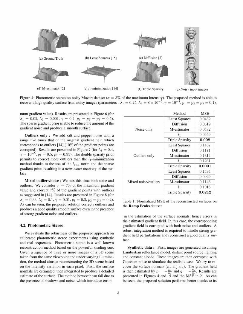
Figure 4: Photometric stereo on noisy Mozart dataset (σ = 3% of the maximum intensity). The proposed method is able torecover a high quality surface from noisy images (parameters : λ1 = 0.25, λ2 = 8× 10⁻⁵, γ = 10−4, p1 = p2 = p3 = 0.1).
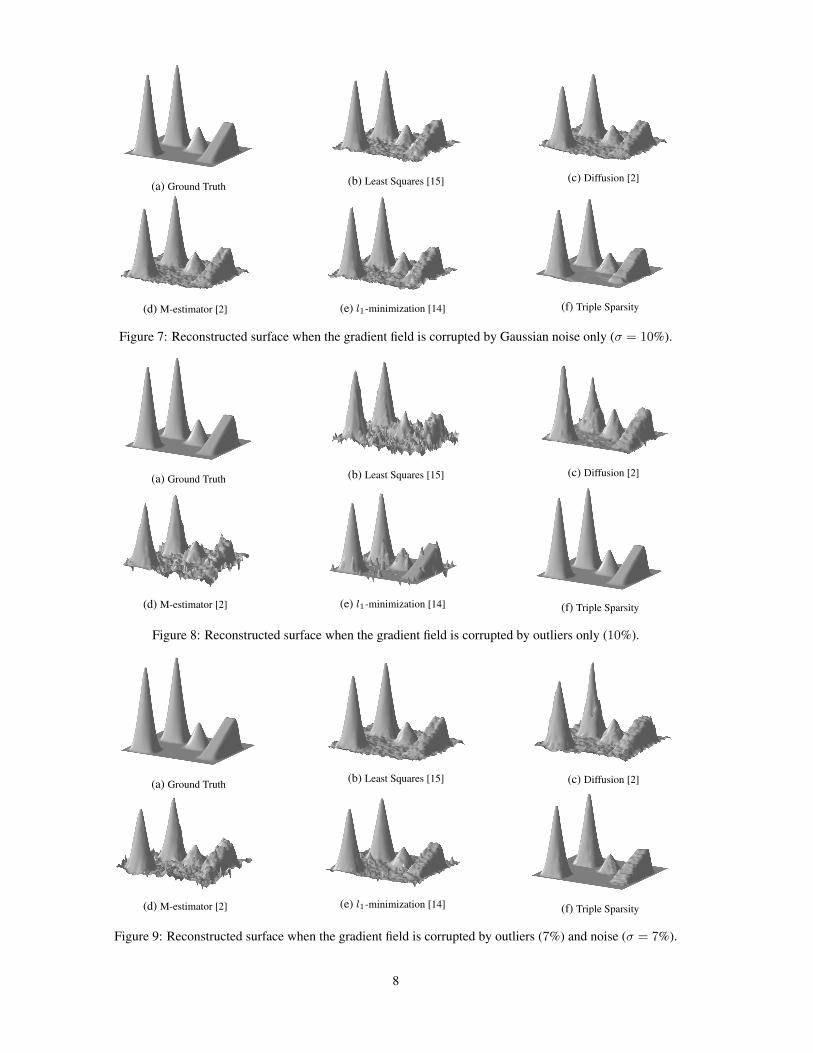
mum gradient value). Results are presented in Figure 6 (forλ1 = 0.05, λ2 = 0.001, γ = 0.4, p1 = p2 = p3 = 0.5).The sparse gradient prior is able to reduce the amount of thegradient noise and produce a smooth surface.
Outliers only : We add salt and pepper noise with arange five times that of the original gradient field whichcorresponds to outliers [14] (10% of the gradient points arecorrupted). Results are presented in Figure 7 (for λ1 = 0.4,γ = 10−5, p1 = 0.5, p2 = 0.95). The double sparsity priorpermits to correct more outliers than the l1-minimizationmethod thanks to the use of the lp<1-norm and the sparsegradient prior, resulting in a near-exact recovery of the sur-face.
Mixed outliers/noise : We mix this time both noise andoutliers. We consider σ = 7% of the maximum gradientvalue and corrupt 7% of the gradient points with outliersas suggested in [14]. Results are presented in Figure 8 (forλ1 = 0.33, λ2 = 0.1, γ = 0.01, p1 = 0.5, p2 = p3 = 0.2).As can be seen, the proposed solution corrects outliers andproduces a good quality smooth surface even in the presenceof strong gradient noise and outliers.
4.2. Photometric Stereo
We evaluate the robustness of the proposed approach oncalibrated photometric stereo experiments using syntheticand real sequences. Photometric stereo is a well knownreconstruction method based on the powerful shading cue.Given a squence of three or more images of a 3D scenetaken from the same viewpoint and under varying illumina-tion, the method aims at reconstructing the 3D scene basedon the intensity variation in each pixel. First, the surfacenormals are estimated, then integrated to produce a detailedestimate of the surface. The method however can fail due tothe presence of shadows and noise, which introduce errors
Method MSELeast Squares 0.0432
Diffusion 0.0519
Noise only M-estimator 0.0482
l1 0.0469
Triple Sparsity 0.008
Least Squares 0.1437
Diffusion 0.1171
Outliers only M-estimator 0.1314
l1 0.1261
Triple Sparsity 0.0001
Least Squares 0.1494
Diffusion 0.0949
Mixed noise/outliers M-estimator 0.1146
l1 0.1016
Triple Sparsity 0.0212
Table 1: Normalized MSE of the reconstructed surfaces onthe Ramp Peaks dataset.
in the estimation of the surface normals, hence errors inthe estimated gradient field. In this case, the correspondinggradient field is corrupted with both noise and outliers. Arobust integration method is required to handle strong gra-dient field perturbations and reconstruct a good quality sur-face.
Synthetic data : First, images are generated assumingLambertian reflectance model, distant point source lightingand constant albedo. These images are then corrupted withGaussian noise to simulate the realistic case. We try to re-cover the surface normals (nx, ny, nz). The gradient fieldis then estimated by p = −nx
nzand q = −ny
nz. Results are
presented in Figures 4 and 5 and the MSE in 2. As canbe seen, the proposed solution performs better thanks to its
5
(a) Ground Truth (b) Least Squares [15] (c) Diffusion [2]
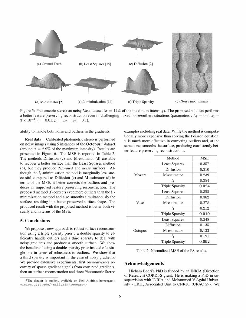
Figure 5: Photometric stereo on noisy Vase dataset (σ = 14% of the maximum intensity). The proposed solution performsa better feature preserving reconstruction even in challenging mixed noise/outliers situations (parameters : λ1 = 0.3, λ2 =3× 10⁻⁴, γ = 0.01, p1 = p2 = p3 = 0.1).
ability to handle both noise and outliers in the gradients.
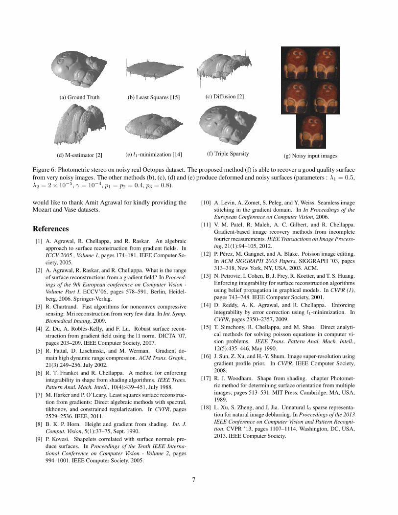
Real data : Calibrated photometric stereo is performedon noisy images using 5 instances of the Octopus 1 dataset(around σ = 2.9% of the maximum intensity). Results arepresented in Figure 6. The MSE is reported in Table 2.The methods Diffusion (c) and M-estimator (d) are ableto recover a better surface than the Least Squares method(b), but they produce deformed and noisy surfaces. Al-though the l1-minimization method is marginally less suc-cessful compared to Diffusion (c) and M-estimator (d) interms of the MSE, it better corrects the outliers and pro-duces an improved feature preserving reconstruction. Theproposed method (f) corrects even more outliers than the l1-minimization method and also smooths simultaneously thesurface, resulting in a better preserved surface shape. Theproduced result with the proposed method is better both vi-sually and in terms of the MSE.
5. ConclusionsWe propose a new approach to robust surface reconstruc-
tion using a triple sparsity prior : a double sparsity to ef-ficiently handle outliers and a third sparsity to deal withnoisy gradients and produce a smooth surface. We showthe benefits of using a double sparsity prior instead of a sin-gle one in terms of robustness to outliers. We show thata third sparsity is important in the case of noisy gradients.We provide extensive experiments, first on near-exact re-covery of sparse gradient signals from corrupted gradients,then on surface reconstruction and three Photometric Stereo
1The dataset is publicly available on Neil Alldrin’s homepage :vision.ucsd.edu/˜nalldrin/research/.
examples including real data. While the method is computa-tionally more expensive than solving the Poisson equation,it is much more effective in correcting outliers and, at thesame time, smooths the surface, producing consistently bet-ter feature preserving reconstructions.
Method MSELeast Squares 0.357
Diffusion 0.310
Mozart M-estimator 0.239
l1 0.354
Triple Sparsity 0.024
Least Squares 0.355
Diffusion 0.362
Vase M-estimator 0.278
l1 0.212
Triple Sparsity 0.010
Least Squares 0.248
Diffusion 0.135
Octopus M-estimator 0.123
l1 0.191
Triple Sparsity 0.092
Table 2: Normalized MSE of the PS results.
AcknowledgementsHicham Badri’s PhD is funded by an INRIA (Direction
of Research) CORDI-S grant. He is making a PhD in co-supervision with INRIA and Mohammed V-Agdal Univer-sity - LRIT, Associated Unit to CNRST (URAC 29). We
Figure 6: Photometric stereo on noisy real Octopus dataset. The proposed method (f) is able to recover a good quality surfacefrom very noisy images. The other methods (b), (c), (d) and (e) produce deformed and noisy surfaces (parameters : λ1 = 0.5,λ2 = 2× 10⁻⁵, γ = 10−4, p1 = p2 = 0.4, p3 = 0.8).
would like to thank Amit Agrawal for kindly providing theMozart and Vase datasets.
References[1] A. Agrawal, R. Chellappa, and R. Raskar. An algebraic
approach to surface reconstruction from gradient fields. InICCV 2005 , Volume 1, pages 174–181. IEEE Computer So-ciety, 2005.
[2] A. Agrawal, R. Raskar, and R. Chellappa. What is the rangeof surface reconstructions from a gradient field? In Proceed-ings of the 9th European conference on Computer Vision -Volume Part I, ECCV’06, pages 578–591, Berlin, Heidel-berg, 2006. Springer-Verlag.
[3] R. Chartrand. Fast algorithms for nonconvex compressivesensing: Mri reconstruction from very few data. In Int. Symp.Biomedical Imaing, 2009.
[4] Z. Du, A. Robles-Kelly, and F. Lu. Robust surface recon-struction from gradient field using the l1 norm. DICTA ’07,pages 203–209. IEEE Computer Society, 2007.
[5] R. Fattal, D. Lischinski, and M. Werman. Gradient do-main high dynamic range compression. ACM Trans. Graph.,21(3):249–256, July 2002.
[6] R. T. Frankot and R. Chellappa. A method for enforcingintegrability in shape from shading algorithms. IEEE Trans.Pattern Anal. Mach. Intell., 10(4):439–451, July 1988.
[7] M. Harker and P. O’Leary. Least squares surface reconstruc-tion from gradients: Direct algebraic methods with spectral,tikhonov, and constrained regularization. In CVPR, pages2529–2536. IEEE, 2011.
[8] B. K. P. Horn. Height and gradient from shading. Int. J.Comput. Vision, 5(1):37–75, Sept. 1990.
[9] P. Kovesi. Shapelets correlated with surface normals pro-duce surfaces. In Proceedings of the Tenth IEEE Interna-tional Conference on Computer Vision - Volume 2, pages994–1001. IEEE Computer Society, 2005.
[10] A. Levin, A. Zomet, S. Peleg, and Y. Weiss. Seamless imagestitching in the gradient domain. In In Proceedings of theEuropean Conference on Computer Vision, 2006.
[11] V. M. Patel, R. Maleh, A. C. Gilbert, and R. Chellappa.Gradient-based image recovery methods from incompletefourier measurements. IEEE Transactions on Image Process-ing, 21(1):94–105, 2012.
[12] P. Perez, M. Gangnet, and A. Blake. Poisson image editing.In ACM SIGGRAPH 2003 Papers, SIGGRAPH ’03, pages313–318, New York, NY, USA, 2003. ACM.
[13] N. Petrovic, I. Cohen, B. J. Frey, R. Koetter, and T. S. Huang.Enforcing integrability for surface reconstruction algorithmsusing belief propagation in graphical models. In CVPR (1),pages 743–748. IEEE Computer Society, 2001.
[14] D. Reddy, A. K. Agrawal, and R. Chellappa. Enforcingintegrability by error correction using l1-minimization. InCVPR, pages 2350–2357, 2009.
[15] T. Simchony, R. Chellappa, and M. Shao. Direct analyti-cal methods for solving poisson equations in computer vi-sion problems. IEEE Trans. Pattern Anal. Mach. Intell.,12(5):435–446, May 1990.
[16] J. Sun, Z. Xu, and H.-Y. Shum. Image super-resolution usinggradient profile prior. In CVPR. IEEE Computer Society,2008.
[17] R. J. Woodham. Shape from shading. chapter Photomet-ric method for determining surface orientation from multipleimages, pages 513–531. MIT Press, Cambridge, MA, USA,1989.
[18] L. Xu, S. Zheng, and J. Jia. Unnatural l0 sparse representa-tion for natural image deblurring. In Proceedings of the 2013IEEE Conference on Computer Vision and Pattern Recogni-tion, CVPR ’13, pages 1107–1114, Washington, DC, USA,2013. IEEE Computer Society.
7
(a) Ground Truth (b) Least Squares [15] (c) Diffusion [2]