Robustness Evaluation of brake systems con- cerned to squeal …€¦ · 2 Brake Squeal: Numerical...

Robustness Evaluation of brake systems con-cerned to squeal noise problem

Ronaldo F. Nunes*, Johannes Will**, Veit Bayer**, Karthik

Chittepu**

*Daimler AG, Sindelfingen ,**Dynardo GmbH, Weimar

Abstract Brakes are one of the most important safety and performance components in automobiles. Appropriately, ever since the advent of the automobile, the devel-opment of brakes has been focused on increasing braking power and reliability. However, the refinement of vehicle acoustics and comfort through improvement in other aspects of vehicle design has dramatically increased the relative contribu-tion of brake noise to these aesthetic and environmental concerns. In order to understand the brake squeal noise problem substantial research has been con-ducted to predict and to reduce its occurrence. Many different factors on both the micro- and macroscopic levels appear to affect squeal. Out of these, important factors are the existence of scatter in material and geometrical properties of the brake system components in reality. Therefore, CAD-based robustness analysis has been carried out while considering the material and geometrical scatter for thorough understanding of brake squeal. The Robustness evaluation is carried out by stochastic modelling of material scatter by random variables and geometrical tolerances by random fields. In regard to the modelling of random fields this paper concentrates on random field generation of one of the components of brake sys-tems to see its effects on the brake squeal noise. Finally, the advantages and disadvantages of the main issues when applying this proposed work flow for brake squeal analysis will be discussed. Keywords: Robustness Evaluation, brake squeal noise, random fields, optiSLang

Weimarer Optimierungs- und Stochastiktage 6.0 – 15./16. Oktober 2009 1

1 Introduction

Brakes are one of the most important safety and performance components in automobiles. Appropriately, ever since the advent of the automobile, the devel-opment of brakes has focused on increasing braking power and reliability. However, the refinement of vehicle acoustics and comfort through improvement in other aspects of vehicle design has dramatically increased the relative contribu-tion of brake noise to these aesthetic and environmental concerns. Brake noise is perceived by customers as both annoying and an indicator of a problem with the brake system. It, in turn, has become one of the major problems causing warranty cost, even though in most cases this type of noise has little or no effect on the performance of the brake system. Therefore, considerable effort has been directed at investigation and reduction of brake noise. Over the years, brake noise has been given various names that provide some definitions of sound emitted such as grind, grunt, moan, groan, squeak, squeal, and wire brush. In order to simplify the discussion, brake noise has been divided into three general categories. The three groups presented are low frequency noise, low frequency squeal and high frequency squeal [1]. Of these phenomena, the one generally termed squeal, is probably the most prevalent, disturbing to both vehicle passengers and the environment, and is expensive to brake and automotive manu-facturers in terms of warranty costs. Therefore, this paper is mainly concerned with brake squeal. In order to understand the brake squeal problem, substantial research has been conducted to predict and eliminate its occurrence. Brakes that squeal do, in gen-eral, not squeal during every braking action. Rather the occurrence of squeal is intermittent or perhaps even random. Many different factors on both the micro- and macroscopic levels appear to affect squeal. Out of these, important factors are the existence of scatter in material and geometrical properties of the brake system components in reality. Therefore, CAD-based robustness analysis has been carried out by considering the material and geometrical scatter for thorough understand-ing of brake squeal. The Robustness evaluation is carried out by stochastic modelling of material scatter by random variables and geometrical tolerances by random fields.

Regarding modelling of random fields this paper is concentrated on random field generation of one of the components of brake system to see its effects on the brake squeal noise. Finally, the advantages and disadvantages of the main issues when applying this proposed work flow for brake squeal analysis will be dis-cussed.


2 Brake Squeal: Numerical Simulation using Complex Eigenvalue Analysis (CEA)

In order to study the brake squeal problem, the finite element method based on complex eigenvalue analysis is applied. The analysis is based on the modelling of a friction contact between brake lining and brake disc in vertical and tangential direction. This provides a coupling with asymmetric stiffness matrix. After that, the instability problem can be evaluated based on stable and unstable vibration in the brake system. For the instability case, a positive real eigenvalue is expected. The magnitude of real eigenvalue is the reference value for the frequency of oc-currence of instabilities. According to Liles [1], this analysis does not draw conclusions regarding the amplitude of oscillation, since the model with initial conditions, i.e. starting condition is considered instead of the one in motion. Slight disadvantage according to Mahajan [2], when compared to the transient analysis, is that the friction coefficient is constant and it can only be varied in new compu-tational runs. According to Liles [1], it can be observed that increase in the friction coefficient most likely leads to an increase in the real eigenvalue of the instabilities. This is due to the rising influence of friction coefficient on the equations. The main ad-vantage of the method lies in the field of modelling. When compared to transient analysis, a clearly improved specification of the brake component is possible in comparable computation time. Therefore, any modification to this model can be carried out in relatively short computational time. This method is hence used to carry out analysis of brake squeal in this paper. Following is the more detailed explanation of complex eigenvalue analysis. Herewith is the first dynamic equation with integrated friction forces.

)()()()( tftxKtxDtxM R=++ &&& (1.1) To generate the instabilities [1], variable normal forces in contact between the brake pad and brake disc are necessary, for example, they can be approximately modelled by spring elements in the FE model. This approach is based, as already mentioned, on the assumption that friction between the brake pad and brake disc is responsible for the emergence of instabilities. The normal forces generate the variable friction forces. Also the friction forces depending on the displacement between the pad and disc can be formulated as

)()()( txKtftf RNR == μ (1.2) From above equation KR is called as stiffness matrix of friction, which consists of the spring stiffness in normal force direction and coefficient of friction μ. Since there are no external forces this can be regarded as exciting force. By combining


the above two equations and rewriting them, the stiffness matrix of friction can be included in general stiffness matrix.

0)()()( * =++ txKtxDtxM &&& (1.3) With )(*

RKKK −= K* thus leads to asymmetric stiffness matrix. Thus calculated complex eigenval-ues are of form

δωλ −±= j or ωδλ j±= (1.4) whereby the real part of complex eigenvalue corresponds to the damping constant of vibration. Due to the asymmetry of stiffness matrix, complex eigenvalues may have positive real parts, i.e. δ>0; which in turn corresponds to the instability of the brake system. This can be easily explained by considering the simple damped system with one degree of freedom. The solution to the equation of motion of a system with one degree of freedom:

0)()()( =++ tKxtxDtxM &&& (1.5) leads to using a exponential form

tt eAeAx 2121

λλ += (1.6) to following

).(cos.)( ϕωδ −= − teAtx Dt (1.7)

This means that the amplitude A, according to an envelope function of e-δ de-creases. However, positive damping constant leads to a corresponding increase in the amplitude values, and an appearance of brakes squeal in practice is likely.

3 Robustness Evaluation

In virtual prototyping it becomes more and more important to check the robust-ness of the system against present scatter of material parameter, geometry or environmental conditions as soon as possible in the design process [3]. Therefore the integration of CAE-based robustness evaluation in the virtual product devel-opment process becomes urgent. For the last 5 years robustness evaluations based on stochastic analysis are implemented successfully into different disciplines in


the automotive industry [4]. The basic idea of robustness evaluation is the creation and evaluation of a set of possible design realisations. The design set represents a scan of the robustness space which is defined by all important scattering input variables.

3.1 Methodology of robustness evaluation In this chapter, Robustness Evaluation using stochastic analysis for productive use will be highlighted. For further detail we refer to literature [3, 4, 5] For the robustness evaluation, optiSLang variance based robustness analysis flow was used. The first important step is the introduction of the scattering input vari-ables with the help of statistical definitions. Because the definition of uncertainties is the essential input to robustness evaluations, the best possible translation of measurements, experience or expectations of scattering variables has to be found.

Fig. 1: The flow of robustness evaluation procedure

The second step is the generation of a representative number of possible design realizations (sampling set). After analyzing every design of the sampling set, the next steps deal with the evaluation of the variation (step 3), importance (step 4) and correlation (step 5) with the help of statistical measurements. It has to be noted that all these statistical measurements are estimated and the confidence, the reliability of the measurements, has to be checked before using them to make design decisions. To make sure that the statistical measurements of variation, importance and correlation are reliable, a certain number of samples is necessary. But the necessary number of runs to estimate the important statistical measure-


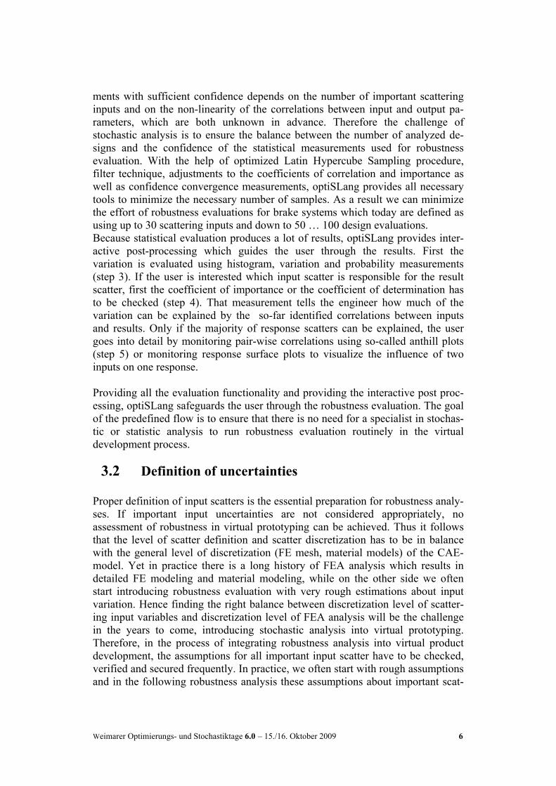
ments with sufficient confidence depends on the number of important scattering inputs and on the non-linearity of the correlations between input and output pa-rameters, which are both unknown in advance. Therefore the challenge of stochastic analysis is to ensure the balance between the number of analyzed de-signs and the confidence of the statistical measurements used for robustness evaluation. With the help of optimized Latin Hypercube Sampling procedure, filter technique, adjustments to the coefficients of correlation and importance as well as confidence convergence measurements, optiSLang provides all necessary tools to minimize the necessary number of samples. As a result we can minimize the effort of robustness evaluations for brake systems which today are defined as using up to 30 scattering inputs and down to 50 … 100 design evaluations. Because statistical evaluation produces a lot of results, optiSLang provides inter-active post-processing which guides the user through the results. First the variation is evaluated using histogram, variation and probability measurements (step 3). If the user is interested which input scatter is responsible for the result scatter, first the coefficient of importance or the coefficient of determination has to be checked (step 4). That measurement tells the engineer how much of the variation can be explained by the so-far identified correlations between inputs and results. Only if the majority of response scatters can be explained, the user goes into detail by monitoring pair-wise correlations using so-called anthill plots (step 5) or monitoring response surface plots to visualize the influence of two inputs on one response. Providing all the evaluation functionality and providing the interactive post proc-essing, optiSLang safeguards the user through the robustness evaluation. The goal of the predefined flow is to ensure that there is no need for a specialist in stochas-tic or statistic analysis to run robustness evaluation routinely in the virtual development process.

3.2 Definition of uncertainties Proper definition of input scatters is the essential preparation for robustness analy-ses. If important input uncertainties are not considered appropriately, no assessment of robustness in virtual prototyping can be achieved. Thus it follows that the level of scatter definition and scatter discretization has to be in balance with the general level of discretization (FE mesh, material models) of the CAE-model. Yet in practice there is a long history of FEA analysis which results in detailed FE modeling and material modeling, while on the other side we often start introducing robustness evaluation with very rough estimations about input variation. Hence finding the right balance between discretization level of scatter-ing input variables and discretization level of FEA analysis will be the challenge in the years to come, introducing stochastic analysis into virtual prototyping. Therefore, in the process of integrating robustness analysis into virtual product development, the assumptions for all important input scatter have to be checked, verified and secured frequently. In practice, we often start with rough assumptions and in the following robustness analysis these assumptions about important scat-


tering input variables are verified and, if necessary, become more detailed. The goal of verification is the ability of the robustness evaluations to forecast a reli-able bandwidth of possible system performance which contains all measurements. For appropriate stochastic definition it becomes necessary to consider the distribu-tion types and information about correlations of single variables as well as it may become necessary to introduce spatially correlated scattering variables.

Fig. 2: Single scattering variable (distribution function, distribution information) and pair-wise correlation between single variables

In case of robustness evaluation of brake systems it is known that the scatter of stiffness of materials is one of the main sources of uncertainty. Especially the pad material shows a high amount of stiffness scatter. Therefore we started our inves-tigation with introduction of scatter of Young’s modulus of different parts. Based on measurements and experience we used conservative estimations for stiffness scatter (see Table1).

3.2.1 Consideration of geometric imperfections Like all production processes, the production process of brake system components has tolerance intervals which will result in scattering geometric dimensions. Thus the simple question of whether the scatter of geometry significantly affects the squeal noise problem arose. To check the robustness of the system against geo-metric imperfections, a process to appropriately introduce the scatter of geometry has to be established.


Component Coefficient of variation (%)

Scatter at 2 Sigma Level of normal distribution

Knuckle 2,50 +/- 5 Rotor 3,00 +/- 6

Calliper 2,50 +/- 5 Calliper Beam 4,00 +/- 8 Steering Rod 2,50 +/- 5 Tension Strut 2,50 +/- 5 Lower Arm 2,50 +/- 5 Wish Bone 2,50 +/- 5

Bolts, Bearings and Hub 2,50 +/- 5 Brake Pad 25,00 +/- 50

Backing Plate 2,50 +/- 5 Steel 2,50 +/- 5

Cast Iron 7,50 +/- 15 Aluminium 2,50 +/- 5

Table 1: Assumptions of stiffness scatter for robustness evaluation

Lower Arm

Wish Bone

Rotor DiscCalliper Beam/Stator

Calliper Housing Steering Rod

Tension StrutKnuckle

Fig. 3: Brake system from front view (Left), rear view (right)


Obviously, the geometry of numerous parts of the brake system is very complex and scattering of single geometric dimensions is very unlikely to have something to do with the real geometric scatter. In this sense, it is important to stress that considering the spatial distribution of geometric scatter, the definition of scatter also will not result in multiple scattering geometry (CAD) variables. In reality it can be seen that tolerances in the production process will result in one or multiple “shapes” representing the parametric of geometry scatter. Therefore we have to identify the imperfection shapes and their amplitudes to appropriately define spatially correlated scattering entities like geometry. For that task the theory of random fields was applied. The base of the identification and definition of scatter are measurements of the geometric deviation of the knuckle of a brake system.

3.2.2 Measurement of geometric deviations of volumetric part, finite element mesh of the perfect geometry, and genera-tion of single imperfect design

The geometry is measured with 3D scan technology, resulting in a triangularised body using STL-format. For an initial study, an imperfect FE model has to be generated from the measurement for further analysis. For this purpose, the coordi-nates of the two models (STL, FE-mesh) have to be transformed to make the coordinate systems coincide.

Fig. 4: left: measurement, differences between the CAD model and the real part

right: finite element model of the CAD model Then each measurement point is assigned to a FE node by node projection tech-nique. Here, a nearest neighbour search provides a sufficient approximation. The FE model as used so far in the analyses represents the perfect knuckle (fig. 4). The surface nodes of the initial FE-Model are grouped in free nodes, which can be moved to fit the measurement and fixed nodes. This cannot be moved for FEM-assembly compatibility reasons. To ensure that the resulting mesh can be used for


FEA of the entire brake system, we did not modify surfaces in contact to other parts. Now “free nodes” are moved according to measured imperfection of measurement points nearest to the FE-node. Because the number of measurement points was smaller than the number of free FE surface nodes, all other nodes on the knuckle surface get imperfections obtained by 3D-Shepard interpolation [8, 10] from the moved surface nodes. Fig. 5 compares the perfect and imperfect CAD and FE models. This may result in collapsed elements (negative Jacobian) or elements with inad-missible aspect ratio, which would produce erroneous analysis results. Therefore a mesh relaxation technique to all surface elements was applied during the genera-tion of the imperfect mesh, relaxing all mid side nodes and deleting too flat elements. Finally, the modified FE mesh of the knuckle which represented the measured geometric body was introduced in the FE brake model and the brake system was analysed. In Fig. 6, the measured imperfect specimen is shown, with colour con-tours representing the imperfection components in Cartesian coordinates.

Fig. 5: Differences between perfect structure and measurement Left, violet: perfect FE model; grey: imperfection FE model Right, orange: perfect FE model, grey: imperfect shaded structure


Fig. 6: Differences between Sample measurements and perfect structure [mm] in Cartesian coordinates.

3.2.3 Generation of random fields, generation of multiple imper-fect designs

After establishing the process to measure one volumetric part and generate one FE representation of the imperfect part, we can apply the process to multiple meas-urements. With the help of random field technology using mean values, standard deviations and spatial correlations of the imperfections obtained from the meas-urements, we can identify the most relevant imperfection shapes and their amplitudes. The random field here is the deviation of the surface of the real, imperfect part from the designed, perfect geometry. It is discretized at the measurement points (see previous section), at which mean values, standard deviations and mutual correlations between the measurement points are evaluated. From this, correlated random variables Xi are defined which represent the statistics of geometrical deviation at each measurement point i. Once a random field is defined as such, simulation of artificial imperfections may substitute further measurements. For the simulation, uncorrelated random vari-ables Yi are needed. These are obtained by a kind of transformation based on eigenvalue analysis of the covariance matrix [8]:


ΨT CXX Ψ = diag{λ} (3.1) Herein, Ψ is the matrix of eigenvectors, stored column-wise, and λ are the respec-tive eigenvalues of CXX. The random field is then generated as a series of shape functions (the eigenvectors of the covariance matrix) multiplied by random ampli-tudes, with variances defined by the eigenvalues. X = Ψ Y (3.2) with components Yi following the Gaussian distribution with mean zero and standard deviation √(λi). Since eigenvalues are usually sorted in a strongly de-creasing order, this offers a way of drastically reducing the number of variables and thus easing the simulation random field realisations for robustness analysis. The simplest first measure is to choose only variables Yi with the highest vari-ances and neglect the remaining set of variables, which do not contribute much to the total scatter of the random field. The ratio of the sum of variances of the con-sidered variables to the total variance of the random field serves as quality measure. In this study, only 10 variables out of 1000 are sufficient to represent 90% of the total scatter. Furthermore, the simulated random variables are post-processed by Robustness methods in optiSLang. Those variables which contribute most to the performance of the analysed part by means of CoD or CoI, correspond to the most relevant imperfection shapes. This helps to further reduce the number of variables in sub-sequent analyses [9, 10]. Each production process, e.g. forging, casting or sheet metal forming has its typical tolerances, which are revealed by examination of the most relevant imperfection shapes of the random field. Fig. 7 provides an over-view on the procedure. Because of cost requirements in the project presented here, only one measurement was available. Consequently, no variances and correlations can be computed. The available information had to be augmented by assumptions and experience. A homogeneous random field for the geometric deviations was assumed independ-ently for the three coordinate directions, i.e., the standard deviation is constant for all points of the random field. It was estimated to 1mm by computing the scatter over all measurement points of the same structure, instead of computing it over a set of measurements. The random field is also assumed isotropic, i.e. the correla-tion between any two points depends on their distance d only. An exponential correlation function was assumed as ρ(d) = exp[-(d/L)2] (3.3) with a correlation length of L = 100mm. The random field is, as mentioned, dis-cretized at the measurement points. After the generation of the random amplitudes, each realization of the random field obtained by eq. (3.2) is mapped to


the surface nodes of the knuckle as described in the previous section. 100 imper-fect structures have been generated that way and submitted to squeal analysis, which is described in section 4. Again, contact surfaces are excluded from the random field. This is also theoretically justified, since contact surfaces are ma-chined and show different, lower tolerances.

Fig. 7: Generation and analysis of random parts

3.2.4 Requirements for Process automation and CAE-Integration using Random Fields

A crucial part of the introduction of geometric scatter is the choice of an appropri-ate parametric for the definition of uncertainties. If the use of single random geometric variables is not suitable, which is definitely the case for complex ge-ometries like the casting parts of brake systems, a parametric using random fields have to be introduced. The random fields represent the variability of geometry and can be defined with assumed shapes and amplitudes, or can be identified from a set of measurements. In any way, the introduction of parametric of geometry variation has high de-mands on the CAE-models and the CAE-process.

- the random fields have to be defined or identified from measurements - imperfect representations of geometry have to be generated - when using mesh modification procedures the modified FE-meshes have

to be relaxed and repaired to fulfil FE stability and accuracy conditions

Model preparation: - map measurement points to structure - define variable surface nodes

Statistics of measurements: means, covariance matrix

X1

X2

Post-process results

Simulate random parameters

Generate set of random specimen, replace in FE assembly to compute


- the compatibility of the modified FE-parts in the ensemble of the FE-model has to be checked (the global FE-model has to allow the geometric variability)

Because of the high demands and the high effort to identify and introduce random field parametric, this level of discretization of spatially correlated scatter will only be implemented when this has a high influence on the robustness of the product performance. But on the other hand, if spatially correlated scatter has a strong influence, appropriate introduction using Random Fields is absolutely necessary to address the robustness evaluation in virtual prototyping. The question of how much effort and cost we will spend in the virtual world should only be discussed in terms of how much costs we face when the robustness problem will not be solved or appear late in the development process.


4 Applications of robustness evaluation

4.1 Robustness evaluation including material uncertain-ties

From the previous experiences in the automotive industry it is known that the scatter of the stiffness of the parts of the brake systems is one of the main scatter sources. It is also known that the stiffness scatter of these parts has a significant influence on the whole brake system behaviour in the aspect of brake squeal. Therefore, robustness evaluation of the brake system is carried out to by introduc-ing the scatter of the Young’s modulus. Based on the measurements and experience, estimation of the stiffness scatter is used as shown in Table 1. The complex eigenvalue analysis of the brake system was performed with NASTRAN NX. The monitoring of instabilities is carried out for two critical eigenfrequencies using two frequency windows around 2 kHz and 6 kHz. The CAE process was introduced into optiSLang and the Robustness analysis is car-ried out using a Latin Hypercube sampling of 100 designs. After calculation, optiSLang was used to perform statistical evaluation and correlation analysis to get a clear picture of the scatter of response parameter resulting from the scatter of design parameters. Squeal propensity in the window around 2 kHz of each of the 100 designs is plotted in Fig. 8. Fig. 8 shows that the variation of all design parameters leads to a high variation is the response parameter which is the squeal coefficient.

Reference modes: 1. 1.46 % @ 1676.2 Hz 2. 1.51 % @ 1859.1 Hz 3. 4.96 % @ 1925.1 Hz

Reference Robustness

Fig. 8: Graphical (left) and Histogram (right) of Squeal Propensity for all De-signs at 2 kHz


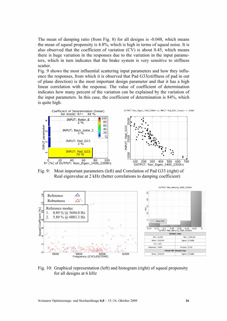
The mean of damping ratio (from Fig. 8) for all designs is -0.048, which means the mean of squeal propensity is 4.8%, which is high in terms of squeal noise. It is also observed that the coefficient of variation (CV) is about 0.45, which means there is huge variation in the responses due to the variation in the input parame-ters, which in turn indicates that the brake system is very sensitive to stiffness scatter. Fig. 9 shows the most influential scattering input parameters and how they influ-ence the responses, from which it is observed that Pad G33(stiffness of pad in out of plane direction) is the most important design parameter and that it has a high linear correlation with the response. The value of coefficient of determination indicates how many percent of the variation can be explained by the variation of the input parameters. In this case, the coefficient of determination is 84%, which is quite high.

Fig. 9: Most important parameters (left) and Correlation of Pad G33 (right) of Real eigenvalue at 2 kHz (better correlations to damping coefficient)


Reference modes: 1. 0.89 % @ 5694.0 Hz 2. 5.89 % @ 6083.3 Hz

Fig. 10: Graphical representation (left) and histogram (right) of squeal propensity for all designs at 6 kHz


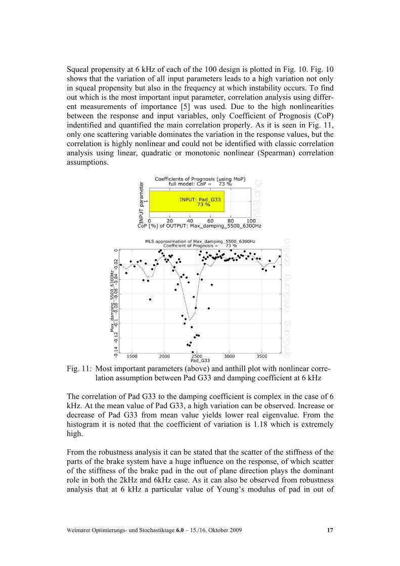
Squeal propensity at 6 kHz of each of the 100 design is plotted in Fig. 10. Fig. 10 shows that the variation of all input parameters leads to a high variation not only in squeal propensity but also in the frequency at which instability occurs. To find out which is the most important input parameter, correlation analysis using differ-ent measurements of importance [5] was used. Due to the high nonlinearities between the response and input variables, only Coefficient of Prognosis (CoP) indentified and quantified the main correlation properly. As it is seen in Fig. 11, only one scattering variable dominates the variation in the response values, but the correlation is highly nonlinear and could not be identified with classic correlation analysis using linear, quadratic or monotonic nonlinear (Spearman) correlation assumptions.

Fig. 11: Most important parameters (above) and anthill plot with nonlinear corre-

lation assumption between Pad G33 and damping coefficient at 6 kHz The correlation of Pad G33 to the damping coefficient is complex in the case of 6 kHz. At the mean value of Pad G33, a high variation can be observed. Increase or decrease of Pad G33 from mean value yields lower real eigenvalue. From the histogram it is noted that the coefficient of variation is 1.18 which is extremely high. From the robustness analysis it can be stated that the scatter of the stiffness of the parts of the brake system have a huge influence on the response, of which scatter of the stiffness of the brake pad in the out of plane direction plays the dominant role in both the 2kHz and 6kHz case. As it can also be observed from robustness analysis that at 6 kHz a particular value of Young’s modulus of pad in out of


plane direction yields a very high damping coefficient, precautions should be taken to avoid this value.

4.2 Robustness evaluation including geometric deviations Geometrical deviations are considered for robustness analysis because in reality there exists some variation in the geometry of each part manufactured, which is why this variation may also influence the responses. In this paper we consider geometric uncertainty of the knuckle (which is a simple part of which to measure its geometry and which is also an important part of the brake system), in order to test the assumption that geometry imperfection may play an important role in the robustness behaviour. From the geometrical measurement of a knuckle it is ob-served (Fig. 5/6) that there is a significant difference between the “perfect CAD geometry” and the real imperfect geometry which is measured. This observation further strengthens the aforementioned assumption . As mentioned previously, the random fields are used for modeling geometrical variation and creating a set of imperfect FE representations of the knuckle. Ro-bustness analysis is carried out for a brake system by replacing the initial FE part with generated imperfect FE-parts of knuckle. Therefore, random fields are ap-plied only for the knuckle part in this paper. Evaluation of robustness analysis is carried out for both the 2 kHz and 6 kHz range. The effect of geometrical tolerance of the geometric imperfection of the knuckle on the squeal propensity in 2 kHz range is given in Fig. 12.


Reference modes: 1. 0.78 % @ 1871.2 Hz 2. 1.83 % @ 1983.7 Hz

Fig. 12: Graphical representation (left) and histogram (right) of squeal propensity

for all designs at 2 kHz Fig. 12 illustrates that the geometrical tolerance has considerable effect on the squeal propensity. It is also observed that most of the designs lie above the refer-


ence. The coefficient of variation is about 0.32 at 2 kHz range, which is high. Thus it can be stated that the geometrical tolerances have considerable effect on the squeal propensity. Therefore they cannot be neglected when quantifying the robustness of the system. As a consequence the coefficient of variation is high which is why it is a sensitive system versus scatter of geometrical tolerance.

Reference

Robustness

Reference modes: 1. 1.64 % @ 5708.2 Hz

Fig. 13: Graphical representation (left) and histogram (right) of squeal propensity

for all designs at 6 kHz

To look at the squeal propensity of 100 designs at 6 kHz see Fig. 13. Fig. 13 indicates that the variation is small. Yet more instability is developed at frequen-cies where the reference run has no instability. The coefficient of variation is about 0,12 at 6 kHz range, which is quite low, yet more instabilities are developed at different frequencies. Therefore it can be stated that geometrical imperfection of the knuckle has small effect on the squeal propensity. From the above analysis it can be concluded that the geometrical imperfections of the components cannot be neglected. However, there can be more effect due to geometrical imperfections of other important components such as caliper and rotor. Therefore, further research has to be carried out in this direction.

5 Summary and Outlook

In this paper, the Robustness evaluation of a Brake System is carried out by sto-chastic modeling of material scatter by random variables and geometrical tolerances by random fields. Regarding modeling of random fields, this paper concentrated on random field generation of one of the components of a typical brake system to see its effects on the brake squeal noise. The main issues arising from the application of random fields were discussed in terms of their advantages and disadvantages for the proposed work flow for the brake squeal analysis.. Based on the results presented, it can be concluded that the geometrical imperfec-tions of the components cannot be completely neglected. For instance, more



complex components, such as brake disc and caliper part must be also taken into account to give more confident results. In general, this paper provides important issues to be considered in the development process of a new brake system and offers a new direction to achieve a more robust system, even in the initial devel-opment phase as a whole.

6 Reference

[1] Liles, G. D, “Analysis of Disc Brake Squeal Using Finite Element Meth-ods”, SAE – Paper No. 891150, 1989.

[2] Mahajan.S, Hu.Y, Zhang.K, “Brake Squeal DOE Using Nonlinear Transient Analysis”, SAE – Paper No. 1999-01-1737, 1999.

[3] Bucher, C.: Basic concepts for robustness evaluation using stochastic analy-sis; Proceedings EUROMECH colloquium Efficient Methods of Robust Design and Optimization, September 2007, London, www.dynardo.com

[4] Will, J.: State of the Art – robustness in CAE-based virtual prototyping processes of automotive applications, Beiträge der Weimarer Optimierungs- und Stochastiktage 4.0, 2007, Weimar, Germany, www.dynardo.com

[5] optiSLang - the Optimizing Structural Language, Version 3.0, DYNARDO, Weimar, 2008, www.dynardo.com

[6] SoS - Statistics_on_Structure, Version 1.1, DYNARDO 2009, Weimar, www.dynardo.com

[7] Will, J.: Bucher, C.: Statistical Measures for the CAE-based Robustness Evaluation, Beiträge der Weimarer Optimierungs- und Stochastiktage 3.0, 2006, Weimar, Germany , www.dynardo.com

[8] Bayer, V.: Random Fields – Theory and Applications. To appear: Beiträge der Weimarer Optimierungs- und Stochastiktage 6.0, 2009, Weimar, Ger-many, www.dynardo.com

[9] Bayer, V.; Roos, D.: Non-parametric Structural Reliability Analysis using Random Fields and Robustness Evaluation. Beiträge der Weimarer Optim-ierungs- und Stochastiktage 3.0, 2006, Weimar, Germany , www.dynardo.com

[10] Bayer, V.; Roos, D.: Efficient Modelling and Simulation of Random Fields. 6th International Probabilistic Workshop, Darmstadt 2008.

http://www.dynardo.com/







Date post:	08-May-2018
Category:	Documents
Upload:	dodiep
View:	215 times
Download:	1 times

Robustness Evaluation of brake systems con- cerned to squeal …€¦ · 2 Brake Squeal: Numerical...

Documents