Rock physics constrained anisotropic WEMVA:

Part I - Theory and synthetic test

Yunyue (Elita) Li, Robert Clapp, Biondo Biondi, and Dave Nichols

ABSTRACT

We present a regularization scheme utilizing available rock physics data to betterconstrain the anisotropic wave-equation migration velocity analysis (WEMVA)and to better resolve the ambiguity among the anisotropic parameters. In ad-dition to the spatial covariance to constrain the spatial correlation of each VTIparameter individually, we propose a cross-parameter covariance at each subsur-face location to link the VTI parameters. There are two significant effects thatthis regularization scheme brings to the updates for the VTI parameters. First,instead of spreading the updates evenly along the wavepath, the regularizationterm allows more updates in the regions where the models are highly uncertain.Second, the regularization term brings extra information for parameter updatesfrom the correlation with the other parameters. These improvements help theinversion converge faster and yield VTI models that are more consistent withthe underlying geological and lithological assumptions. We demonstrate theseimprovements on a synthetic dataset.

INTRODUCTION

Anisotropic model building tries to resolve more than one parameter at each modellocation. This number is three for a vertical transverse isotropic (VTI) medium,and five for a tilted transverse isotropic (TTI) medium. Traditional surface seismictomography may be able to produce an accurate isotropic earth model efficiently fora large area when the acquisition is dense and the earth is well-illuminated by rays ata wide range of angles. However, surface seismic data inversion becomes ill-posed andhighly underdeterimined due to the rapidly increasing model space with the increasingcomplexity of the subsurface.

One important disadvantage of surface seismic tomography is its lack of depth in-formation. During tomography, neither the low wavenumber velocity nor the highwavenumber reflectivity are known. This issue is more severe when we consideranisotropy. Several localized tomography around the wells were studied to add thedepth dimension into the inversion (Bear et al., 2005; Bakulin et al., 2010b,a). Jointinversion of surface seismic data and borehole data (check-shots and walkaway VSPs)in these studies helps to yield better defined earth models. Due to the ambigu-

SEP–152

Li et al. 2 Rock physics constrained WEMVA

ity among the parameters, it is difficult to resolve a reliable and unique anisotropicmodel in 3D even with the borehole aided localized tomography (Bakulin et al., 2009).

In the anisotropic case, the uncertainties are further increased because the sen-sitivities of the kinematics of the surface seismic data to the anisotropic parametersare much lower than to velocity. Large offsets and a wide range of illumination anglesare required to constrain the anisotropic parameters. Consequently, the recoverabledepth range for the anisotropic parameters is much shallower than when a simpleisotropic velocity is estimated. Even in the shallow region, where the seismic wavestravel with wide angles and large offsets, the kinematic effects of the velocity can stilloverwhelm the inversion.

To help with the inversion for anisotropy, we can use our prior knowledge of thesubsurface. In addition to the two-point (spatial) covariance describing the smooth-ness in the subsurface (Clapp, 2000; Woodward et al., 2008; Li and Biondi, 2011),a single point (local) cross-parameter covariance can be used to better describe thesubsurface. One way to estimate the cross-parameter covariance is from rock physicsstudies (Hornby et al., 1995; Sayers, 2004, 2010; Bachrach, 2010b). Many authors(Dræge et al., 2006; Bandyopadhyay, 2009; Bachrach, 2010a) have built depth trendsfor seismic purposes. In particular, Bachrach (2010a) developed both deterministicand stochastic modeling schemes based on the rock physics effective-media models forcompacting shale and sandy shale. The stochastic modeling enables us to explore therange of possible anisotropic parameters based on the rock physics modeling parame-ters. Further corroborated by core measurements, the parameters allowed by the rockphysics model are limited to a certain range, which greatly reduces the possible rangeof the VTI parameters. These rock physics modeling results can be used to constructinitial VTI models and the covariance relationships among the VTI parameters. Liet al. (2011) and Yang et al. (2012) have demonstrated that the rock physics priormodels are helpful in constraining ray-based tomography.

In this paper, we first analyze the sensitivities of the WEMVA objective func-tion with respect to different VTI parameters in a homogeneous VTI model. Us-ing an interpolation example, we demonstrate the additional information that thecross-parameter covariance brings to the inversion. We then test three different reg-ularization schemes when a synthetic dataset is inverted using anisotropic WEMVA.The inversion results show that when the accurate full covariance matrix is applied,the convergence of the WEMVA inversion as well as the lithological definition of theinverted models are improved.

WEMVA AND ROCK-PHYSICS REGULARIZATION

Anisotropic WEMVA aims at building an anisotropic earth model that minimizes theresidual image from the surface seismic data (Li and Biondi, 2011). This optimizationproblem is highly nonlinear and underdetermined. We commonly add a model reg-ularization term to the anisotropic WEMVA objective function defined in the image

SEP–152

Li et al. 3 Rock physics constrained WEMVA

space to constrain the null space and stabilize the inversion. Our resulting objectivefunction is:

S(m) =1

2||DθI(x, θ)||−α

1

2||

∑θ

I(x, θ)||+β1

2(m−mprior)

TC−1M (m−mprior), (1)

where the first two terms define the “data fitting” objective, and the third definesthe “model regularization” objective. The first term is to minimize the differentialsemblance in the data fitting objective, and the second term is to maximize thestacking power. Model m is the VTI subsurface model, I(x, θ) is the migration imagein the angle domain with θ the aperture angle and Dθ a derivative operator along theangle axis. In the model regularization objective, mprior and CM define a Gaussiandistribution of a prior model that is ideally independent of the seismic data. Thisregularization will bring more information into the optimization. Parameters α andβ balance the relative weights among different objectives.

The data fitting objective relates the incoherence in the angle domain commonimage gathers to the inaccuracy in the subsurface models. To test the data objectives,we model a simple synthetic dataset using a homogeneous VTI model (vv = 2 km/s,ε = 0.2, and δ = 0.1) with one flat reflector. The maximum offset is 6 km, andthe depth of the reflector is 1.5 km. The data are then migrated using all possiblecombinations of vv, ε, and δ when vv varies in [1.5, 2.5] km/s, ε ∈ [0.1, 0.3], andδ ∈ [0, 0.2]. Based on the migrated images in the angle domain, the data fittingobjective at each model point in this subspace is then computed according to the firsttwo terms in Equation 1.

Figure 1 shows the data fitting objective function assuming one of the three VTIparameters is accurate. Panels (a), (b), and (c) are extracted from the vv = 2km/splane, δ = 0.1 plane, and ε = 0.2 plane, respectively. When the third parameteris accurate, the data fitting objective function is convex and comes to a minimumat the correct solution for the other two parameters. However, the resolution of theobjective function with respect to each parameter is dramatically different. A muchhigher resolution for velocity than for ε and δ can be seen from Figures 1(b) and (c).The resolution of ε and δ is at least an order of magnitude lower than that of velocity(notice the smaller range of values on the colorbar in Figure 1(a)).

Moreover, severe tradeoffs among the VTI parameters can be observed from Figure1. A strong tradeoff can be seen in Figure 1(a). The WEMVA objective functioncannot resolve ε or δ independently as long as the summation of the two remains thesame (unless events propagating at more than 60◦ angles are recorded). Tradeoffsbetween the anisotropic parameters and the vertical velocity can also be seen fromFigures 1(b) and 1(c), where positive vertical velocity errors are compensated bynegative errors in the anisotropic parameters and vice versa. Nevertheless, thesetradeoff effects are much less obvious, further demonstrating the low sensitivity ofseismic data to the anisotropic parameters.

For pressure waves, velocity has a dominant effect on the kinematics due to itsfirst-order influence. As a result, the objective function is biased towards the velocity

SEP–152

Li et al. 4 Rock physics constrained WEMVA

Figure 1: The value of data fitting objective function extracted from (a) vv = 2 km/splane, (b) δ = 0.1 plane, and (c) ε = 0.2 plane. Notice the different color scale inpanel (a). [CR]

Figure 2: The value of data fitting objective function extracted from (a) vv = 1.9km/s plane, (b) vv = 2 km/s plane, and (c) vv = 2.1 km/s plane. [CR]

SEP–152

Li et al. 5 Rock physics constrained WEMVA

error despite the error in the other VTI parameters. Figure 2 shows the topographyof the data fitting objective function extracted from the (a) vv = 1.9 km/s plane, (b)vv = 2 km/s plane, and (c) vv = 2.1 km/s plane, respectively. When the velocity isinaccurate, the objective function loses its convexity in the ε–δ plane. The objectivefunction always dips towards higher ε and higher δ when velocity is slower, andtowards lower ε and lower δ when velocity is faster. In these cases, the gradient of theobjective function would not be able to guide the inversion to the correct solution forthe anisotropic parameters if the errors in ε and δ are in the opposite direction thanthe velocity error.

For field data, the “data fitting” objective function has worse behavior because thestructure of the earth subsurface is highly complex with heterogeneities at all scalesand densely distributed dipping reflectors. These complexities weaken the convexityof the objective function and create local minima.

To better constrain the model and to mitigate severe ambiguities among the VTIparameters, we include additional information in the inversion. We utilize the regu-larization term in Equation 1 by assuming a multivariate Gaussian distribution forthe VTI model parameters. To speed up the convergence, we use a preconditioningscheme instead of the original regularization scheme.

WEMVA with the rock physics regularization

Assuming a Gaussian distribution, Tarantola (1984) characterizes the prior informa-tion using the mean and the covariance of the model and includes it as a regularizationterm. We separate the covariance into two parts: a spatial covariance between thesame parameter at different locations, and a cross-parameter covariance between dif-ferent parameters at the same location.

The spatial covariance is mainly defined by the structure of the area, and it can beestimated using a set of steering filters (Clapp, 2000). The cross-parameter covariancecan be inferred from the lithological information at the model location. In a previouswork (Li et al., 2013), we introduced the cross-parameter matrix with only diagonalterms due to the lack of the lithological information. This diagonal preconditioningbalances the relative scales among the VTI parameters, but it ignores the correlationamong them.

When we have a rough estimate of the lithological environment, we can build amore complete cross-parameter covariance using rock physics modeling. As an ex-ample, the Gulf of Mexico is populated with large shale deposits. Therefore, rockphysics principles can be used to estimate the range of anisotropic parameters con-sidering a compacting shale model (Bachrach et al., 2011). As demonstrated in (Liet al., 2014), the rock physics stochastic modeling for shale anisotropy shows that inthe shallow sediments, a high velocity zone is generally collocated with sand layerswhere the anisotropy is low. On the contrary, diagenesis processes in the more com-pacted deeper sediments alter the clay mineral from smectite to illite, which increases

SEP–152

Li et al. 6 Rock physics constrained WEMVA

both velocity and anisotropy simultaneously. Valuable prior knowledge about thesubsurface can be included in the inversion via both the diagonal and the off-diagonalterms in the cross-parameter covariance matrix.

We assume the spatial covariance and local cross-parameter covariance compo-nents are independent of each other (Li et al., 2011). To speed up the convergence,we use a preconditioning scheme where we use steering filters to approximate thesquare-root of the spatial covariance, and a standard-deviation matrix to approxi-mate the square-root of the cross-parameter covariance.

Mathematically, the preconditioning variable n is related to the original model mas follows:

m = ΣSn. (2)

In Equation 2, the smoothing operator S is a band-limited diagonal matrix:

S =

∣∣∣∣∣∣Sv 0 00 Sε 00 0 Sδ

∣∣∣∣∣∣ , (3)

with potentially different smoothing operators for velocity, ε, and δ, according to thegeological information in the study area. The standard deviation matrix Σ is thesquare-root of the covariance matrix:

Σ =

∣∣∣∣∣∣Cvv I Cvε I Cvδ ICεv I Cεε I Cεδ ICδv I Cδε I Cδδ I

∣∣∣∣∣∣1/2

. (4)

The diagonal elements Cvv, Cεε, and Cδδ denote the variance of the velocity, ε, andδ, respectively. The off-diagonal elements Cvε, Cvδ, and Cεδ denote the cross-variancebetween the velocity and ε, between velocity and δ, and between ε and δ, respectively.These elements can be obtained by rock-physics modeling and/or lab measurements(Bachrach et al., 2011; Li et al., 2011). The covariance matrix Σ is symmetric. Asa result, there are only six independent components in the covariance matrix. In anideal case, matrix Σ should be estimated at each subsurface location to reflect thelocal lithological information.

Interpolation test with the preconditioning operators

To demonstrate the extra information that the preconditioning operators introduceto the inversion, we test these preconditioners on a classic missing data problem(Claerbout, 2009) on the BP2007 model. Consider the synthetic example in Figure 3,where the left column shows the current best spatial estimation of the VTI parameters(initial model) and the right column shows the true VTI parameters (true model). Tobuild the initial velocity model, we assume the water bottom topography is knownand the water velocity is 1.5 km/s. The basement interface is assumed to be flat

SEP–152

Li et al. 7 Rock physics constrained WEMVA

and the velocity of the basement rock is 3.5 km/s. Then, we linearly interpolate thevelocity between the water bottom and the basement interface. We follow a similarapproach to build the initial ε and δ model. The resulting initial VTI model showssmooth, linearly increasing trends for velocity, ε, and δ.

The true velocity, ε, and δ updates are plotted in Figures 4(a), (b) and (c), re-spectively. The true velocity updates show two anticline structures up shallow anda major anticline structure down deep. The updates in the anisotropic parameterscontain more layering information than the velocity update. These are the solutionsto the model building problem.

Suppose that, among the three unknown parameters, only velocity has been mea-sured at random well locations in this section (Figure 4(d)). The goal of the inversionis to interpolate the well information onto a regular 2D grid and to provide reasonableestimates for the unmeasured anisotropic parameters.

The interpolation problem can be formulated as a data fitting objective

WBd ≈ Wm; (5)

to match the interpolated model m with the binned data Bd at the well locationdefined by W. Additionally, the distribution of the model must follow a user-definedprior covariance C:

0 ≈ C−1/2m. (6)

To speed up the inversion, a preconditioning strategy is used by introducing a pre-conditioning variable

n = C−1/2m. (7)

Now, the system of equations we solve is as follows:

WB d ≈ WC1/2n; (8)

0 ≈ n. (9)

Different choices can be made for the preconditioner C1/2. As discussed in the pre-vious work (Li et al., 2013), structure dip filters can be good estimates of the spatialcovariance of the velocity and anisotropic model individually. Figure 5 shows a stackedimage of the studied area (panel (a)) and the dip field estimated from it (panel (b)).Steering filters Sv (Clapp, 2000) are estimated at each point on this section accordingto the dip field. We use the same steering filters for ε and δ; that is Sε = Sδ = Sv.

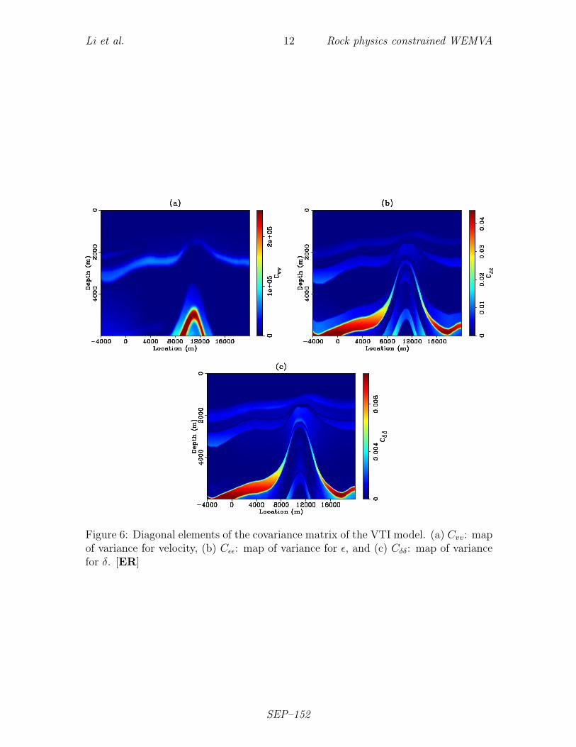
In addition, we observe correlations among the VTI parameters at a single loca-tion. Point-by-point, we calculate the variance and the cross-variance using the trueupdates in Figure 4, and we plot the six independent components of the covariancematrix in Figure 6 and 7. The diagonal components in Figure 6 describe the spatialdistribution of the variance between the initial and true model for each VTI param-eter. The off-diagonal components in Figure 7 describe the cross-covariance betweentwo given VTI parameters.

SEP–152

Li et al. 8 Rock physics constrained WEMVA

Figure 3: Comparison of the initial (left column) and the true (right column) modelsfor BP2007 synthetic test. Top row: velocity models; middle row: ε models; bottomrow: δ models. [CR]

SEP–152

Li et al. 9 Rock physics constrained WEMVA

Figure 4: True updates in velocity in (a), ε in (b) and δ in (c). Pseudo velocity logsat random locations are plotted in (d). [CR]

SEP–152

Li et al. 10 Rock physics constrained WEMVA

To demonstrate the value of the cross-parameter covariance, we compare the in-version results of the following two preconditioners:

C1/21 = S, (10)

and

C1/22 = SΣ. (11)

The interpolation results of both tests after six iterations are plotted in Figure 8.

The interpolation result for velocity using C1/21 is shown in Figure 8(a). We do

not plot the interpolation results for ε and δ because both of them are zero due to thelack of measurements. The inversion results are better to the right side of the sectionwhere the velocity logs are denser. The shallow sand layer has been almost perfectlyrecovered. On the left side, the inversion interpolates between and extrapolates fromthe well logs along the structural dip. The result hints at the shallow sand layer andthe deep anticline structure. However, the blank spaces between the logs are too largeto be filled.

The inverted velocity using C1/22 (Figure 8(b)) is very similar to that using C

1/21 .

However, extra information added by the off-diagonal terms in the covariance matrixshows correct updates in the inverted results for ε and δ. On the right side, theinversion almost perfectly recovers the ε and δ updates along with the proper layeringin both the shallow and the deep sections. The reconstruction of the deep layeringis mostly attributed to the accurate correlation between velocity and the anisotropicparameters. To the left, the correct ε and δ updates are obtained wherever the velocityhas been correctly resolved. In the regions where velocity is missing, the off-diagonalterms do not falsely “create” updates for ε and δ.

SEP–152

Li et al. 11 Rock physics constrained WEMVA

Figure 5: A stacked image of the studied area in panel (a), and the correspondingdip field in panel (b). [CR]

SEP–152

Li et al. 12 Rock physics constrained WEMVA

Figure 6: Diagonal elements of the covariance matrix of the VTI model. (a) Cvv: mapof variance for velocity, (b) Cεε: map of variance for ε, and (c) Cδδ: map of variancefor δ. [ER]

SEP–152

Li et al. 13 Rock physics constrained WEMVA

Figure 7: Off-diagonal elements of the covariance matrix of the VTI model. (a) Cvε:map of covariance between velocity and ε, (b) Cvδ: map of covariance between velocityand δ, and (c) Cεδ: map of covariance between ε and δ. [ER]

SEP–152

Li et al. 14 Rock physics constrained WEMVA

Figure 8: Comparison of the interpolation results. (a): Inverted velocity using C1/21 .

(b): Inverted velocity using C1/22 . (c): Inverted ε using C

1/22 . (d): Inverted δ using

C1/22 . [CR]

SEP–152

Li et al. 15 Rock physics constrained WEMVA

WEMVA SYNTHETIC EXAMPLE WITH ROCKPHYSICS CONSTRAINTS

In this section, we will test the preconditioning scheme using different estimations ofthe covariance matrix on the modified BP2007 VTI dataset. The synthetic data aremodeled with a streamer geometry where the maximum offset is 6km. Shot spacingis 100m, and receiver spacing is 12.5m. A total of 100 shots have been modeled.The synthetic data are then inverted using the preconditioned anisotropic WEMVAtechnique.

The initial and the true models are shown in Figure 3. Compared with the truemodels, the initial model captures the overall increasing trend of the VTI parameters.However, the following two important lithological layers in the shallow region (above4km) are missing from the initial models: the first shale layer with low velocity andhigh anisotropy, and the third sand layer with high velocity and low anisotropy. Thesand-shale inter-layering in the deep region (below 4km) is obvious along the anticlinein the true model. In contrast with the shallow region, the high velocity layers in thedeep section correlate with the shale layers and with high anisotropy. Because thedeeper structures below 4km will be difficult to resolve due to the limited acquisition,we will focus our discussion on the shallow sediments.

The initial migration image is shown in Figure 9. There are large vertical shiftsbetween the initial image and the true image. The reduced amplitudes in the deeperregion on the initial stacked image indicate a weaker focusing effect compared withthe true stacked image. Figure 10 shows the comparison of the initial ADCIGs in (a)with the true ADCIGs in (b). The upward moveouts in the initial ADCIGs indicatethat the average migration velocity is lower than the true average velocity along thewavepaths. Although the true anisotropy updates in the sand layer are negative bymy construction, the overwhelming effects of the slower velocity on the kinematics ofthe acoustic waves are predominant. In the iterative WEMVA process, these upwardmoveouts in the ADCIGs will translate into positive updates in both velocity andanisotropic parameters ε and δ.

The six independent components of the covariance matrix at each point are plottedin Figures 6 and 7. Notice the negative correlation between velocity and anisotropyin the shallow region, and the positive correlation in the deep region (Figure 7(a) and7(b)). Figure 7(c) shows that the positive correlation trend between ε and δ is largelyindependent of the depth in this section.

To test the effect of different preconditioning schemes, we perform anisotropic

SEP–152

Li et al. 16 Rock physics constrained WEMVA

Figure 9: Comparison of the initial stacked image (a) and the true stacked image (b).Notice the depth shift between the images and the unfocused reflectors around z = 3km and x = 4 km. [CR]

SEP–152

Li et al. 17 Rock physics constrained WEMVA

Figure 10: Comparison of the initial ADCIGs (a) and the true ADCIGs (b). Noticethe upward moveout throughout the section in the initial gathers. [CR]

SEP–152

Li et al. 18 Rock physics constrained WEMVA

WEMVA with three different preconditioning matrices:

Σ1 =

∣∣∣∣∣∣I 0 00 I 00 0 I

∣∣∣∣∣∣1/2

, (12)

Σ2 =

∣∣∣∣∣∣Cvv I 0 0

0 Cεε I 00 0 Cδδ I

∣∣∣∣∣∣1/2

, (13)

Σ3 =

∣∣∣∣∣∣Cvv I Cvε I Cvδ ICεv I Cεε I Cεδ ICδv I Cδε I Cδδ I

∣∣∣∣∣∣1/2

. (14)

The preconditioning matrix Σ1 indicates that no preconditioning is applied; Σ2 in-dicates that a diagonal preconditioning is applied; and Σ3 indicates that the fullpreconditioning approach is applied. The spatial covariance matrix for the threetests are the same.

The initial preconditioning model n0 is obtained by minimizing the following ob-jective function:

Jinit =1

2〈m0 −ΣBn0,m0 −ΣBn0〉 . (15)

The gradient of the WEMVA objective function (1) with respect to this precondi-tioning variable n is

∇nJ = (∂m

∂n)∗∇mJ

= B∗Σ∗∇mJ, (16)

where ∇mJ = [∇vJ ∇εJ ∇δJ ]T .

To understand the preconditioning scheme, we analyze the preconditioning effectassuming a nonlinear steepest decent inversion framework. The initial preconditionedmodel n0 is obtained by minimizing the following objective function:

Jinit =1

2〈m0 −ΣSn0,m0 −ΣSn0〉 . (17)

For the ith iteration, the preconditioned variable is obtained by

ni+1 = ni + λi∇nJ, (18)

with λi the step length in the ith iteration. Hence the original model variable is

mi+1 = SΣni+1

= SΣni + λiSΣ∇nJ

= mi + λiSΣΣ∗S∗∇mJ. (19)

SEP–152

Li et al. 19 Rock physics constrained WEMVA

Equation 19 suggests that preconditioning a non-linear inversion is equivalent to filter-ing the gradients so that the resulting updates have the desired spectrum. Therefore,instead of explicitly reformulating the preconditioned inversion, we can make use ofthe original non-linear conjugate gradient algorithm implementation with minimalchanges. The preconditioning step is highlighted in red in Algorithm 1.

Algorithm 1 Optimization algorithm

initialize the model: m0

compute the migrated image: I0

compute the gradient: g0

precondition the gradient: g0s = SΣΣ∗S∗g0

initialize the search direction: p0 = −g0s

for k = 1 · · ·Nk doperform a line search: optimize λ, argmin

λJ(mk−1 + λpk−1)

update the velocity model: mk = mk−1 + λpk−1

compute the migrated image: Ik

compute the gradient: gk

precondition the gradient: gks = SΣΣ∗S∗gk

find the search direction: pk = −gk + (gks )T (gk

s−gk−1s )

(gk−1s )T gk−1

s

end for

Inversion results

Figure 11 shows the velocity updates after the first iteration. In panel (a), we displaythe raw update from the moveouts on the ADCIGs. The overall update direction forvelocity is positive. The vertical resolution of the updates is very low after the firstiteration: a bulk positive velocity shift is indicated by the raw gradient. In panel(b), the spatial distribution of the velocity update has been modified by the diagonalelements of the covariance matrix. Because of the prior knowledge of a sand layerwith high velocity perturbation, the preconditioning concentrates the strong velocityupdate within that layer. Compared with the true velocity update in panel (d),the velocity update with the diagonal preconditioning already achieves high verticalresolution from the first iteration. In panel (c), we utilize all the elements of thecovariance matrix to precondition the gradient. The resulting update is very similarto the update with diagonal preconditioning. This similarity suggests that the off-diagonal elements of the covariance matrix have limited influence on velocity.

Figure 12 shows the updates in ε after the first iteration. In panel (a), the rawupdate in ε appears lower resolution than the raw updates for velocity. All theupdates are in the positive direction, thus compensating for the upward moveoutsin the initial ADCIGs. However, the updates in ε are very small due to its lowinfluence to the kinematics of the waves. Although the diagonal preconditioning haschanged the spatial distribution of the update with better definition of the layers,

SEP–152

Li et al. 20 Rock physics constrained WEMVA

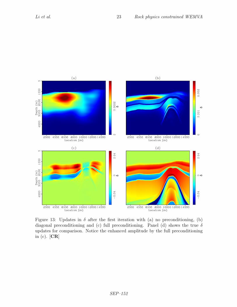
the positive values in the ε update in the sand layer is still in the opposite directionof the true update (Figure 12b). In panel (c), when the off-diagonal elements ofthe covariance matrix are included to account for the cross-variance between velocityand ε, the preconditioning provides ε updates in accordance with the lithology asfollows: positive ε updates in the shale layer and negative ε updates in the sand layer.Considering the significant difference between panel (b) and panel (c), we concludethat the lithological information mainly comes from the off-diagonal elements of thecovariance matrix. Similar analysis and conclusions can also be made for anisotropicparameter δ (Figure 13).

Figure 14 shows the updates in velocity after 20 iterations. Panel (a) shows thevelocity update when no preconditioning is applied. The spatial resolution for velocitygradually improves with iterations. However, the resolution remains significantlylower than the true update at iteration 20. More iterations could further improve theresolution, with a higher weighting on the stacking power term. However, to make afair comparison, we stop all the tests at 20 iterations. When implementing diagonalpreconditioning (panel (b)) and full preconditioning (panel (c)), the overall structureand resolution of the velocity updates remain stable with increasing iterations. Thisshows an early convergence. Nevertheless, the later iterations improve the definitionof the thin sand layer with high velocity at z = 1.5km and x = 10km, and theanticline structure with low velocity around z = 4km and x = 11.5km. The finalinversion results for velocity are nearly identical between the diagonal and the fullpreconditioning schemes. As will be shown by the final stacked image, the effectiveimaging velocity from the three different preconditioning schemes are very similar.

Figure 15 shows the updates in ε after 20 iterations. When no preconditioningis applied (panel (a)), the resolution of the ε is lower than the resolution of veloc-ity as predicted by the topography of the objective function in the previous section.Compared with Figure 14(a), although the updates in ε in Figure 15(a) are mostlyin phase with the updates in velocity, the positive updates on the flanks and the topof the anticline are in the correct direction despite the negative velocity updates atthe same locations. When preconditioned with diagonal covariance (panel (b)), theinversion has a better resolution for the shale layer near the water bottom. However,the updates in the sand layer are in the opposite direction of the true ε updates.The inverted updates for ε are very close to the true updates when the off-diagonalcomponents of the covariance matrix are also included in the preconditioning (panel(c)). The inversion almost perfectly recovers both the shale and the sand layer due tothe prior knowledge of the cross-correlation between the velocity and ε perturbationwithin each layer. Similar analysis and conclusions can also be made for the invertedupdates in δ (Figure 16). Notice that on the flanks and the top of the anticline, theinversion successfully resolves the ε perturbation no matter which preconditioningscheme is applied. This success is due to the rich angular coverage in these regions,especially wide angle imaging rays with higher sensitivity to the anisotropic parame-ters.

Figure 17 shows the inverted vertical velocity models after twenty iterations.

SEP–152

Li et al. 21 Rock physics constrained WEMVA

vv (m

/s)

vv (m

/s)

Figure 11: Velocity updates after the first iteration with (a) no preconditioning,(b) diagonal preconditioning and (c) full preconditioning. Panel (d) shows the truevelocity updates for comparison. [CR]

SEP–152

Li et al. 22 Rock physics constrained WEMVA

εε

εεε

Figure 12: Updates in ε after the first iteration with (a) no preconditioning, (b)diagonal preconditioning and (c) full preconditioning. Panel (d) shows the true εupdates for comparison. Notice the enhanced amplitude by the full preconditioningin (c). [CR]

SEP–152

Li et al. 23 Rock physics constrained WEMVA

δδ δ

δ

Figure 13: Updates in δ after the first iteration with (a) no preconditioning, (b)diagonal preconditioning and (c) full preconditioning. Panel (d) shows the true δupdates for comparison. Notice the enhanced amplitude by the full preconditioningin (c). [CR]

SEP–152

Li et al. 24 Rock physics constrained WEMVA

Figure 14: Velocity updates after twenty iterations with (a) no preconditioning, (b)diagonal preconditioning and (c) full preconditioning. Panel (d) shows the true ve-locity updates for comparison. [CR]

SEP–152

Li et al. 25 Rock physics constrained WEMVA

Figure 15: Updates in ε after twenty iterations with (a) no preconditioning, (b)diagonal preconditioning and (c) full preconditioning. Panel (d) shows the true εupdates for comparison. [CR]

SEP–152

Li et al. 26 Rock physics constrained WEMVA

Figure 16: Updates in δ after twenty iterations with (a) no preconditioning, (b)diagonal preconditioning and (c) full preconditioning. Panel (d) shows the true δupdates for comparison. [CR]

SEP–152

Li et al. 27 Rock physics constrained WEMVA

When no preconditioning is applied (panel (a)), the inversion only recovers lowwavenumber components of the velocity model. When diagonal or full precondi-tioning is applied (panels (b) and (c), respectively), the layering with variable depthsin the shallow region is very well recovered. In the deeper section, only the stronglow velocity anomaly at the top of the anticline has been retrieved due to the limitedangle illumination. The lack of inversion success in the deeper region suggests thatpowerful as our preconditioning scheme is, it cannot “create” information where theseismic data has little information.

Figure 18 shows the inverted ε models after twenty iterations. Inversions withoutthe cross-parameter correlation (panel (a) and (b)) have barely moved the solutionfrom the initial models. The inversion can resolve a high resolution and rock physicsplausible ε model only when the full preconditioning scheme is applied.

Figure 19 shows the inverted δ models after twenty iterations. Similar to theinversion results for ε, the information contributed by the off-diagonal terms in thefull covariance matrix provides much better spatial and rock physics constraints.Notice that in the shallow shale layers, the stronger anisotropic thin shale layers arevery well resolved on panel (c). This high resolution result is attributed to boththe high resolution preconditioning and the high resolution stacking power objectivefunction.

It is important to note that some ambiguities remain in the VTI parameters evenwhen the full preconditioning scheme is used. One example is highlighted by the el-lipses in the figures. In Figure 17(c), a low velocity wedge can be seen when comparedwith the true velocity model in Figure 17(d). In the corresponding region, a thin-ner isotropic sand layer has been observed from the inverted anisotropic parameters(Figures 18(c) and 19(c)) when compared with the true models (Figures 18(d) and19(d)). The low velocity anomaly and the high anisotropic anomalies, although ofdifferent shapes, compensate each other and focus the seismic data associated withthis area.

Figure 20 shows the comparison between the final stacked images produced bydifferent preconditioning schemes with the true stacked image. All three invertedimages are greatly improved from the initial stacked image in Figure 9(a) with betterfocusing and better defined depths of the reflectors. Despite the significant differencesin the inverted velocity and anisotropic models from three preconditioning schemes,the effective imaging velocities along the wavepaths are very similar.

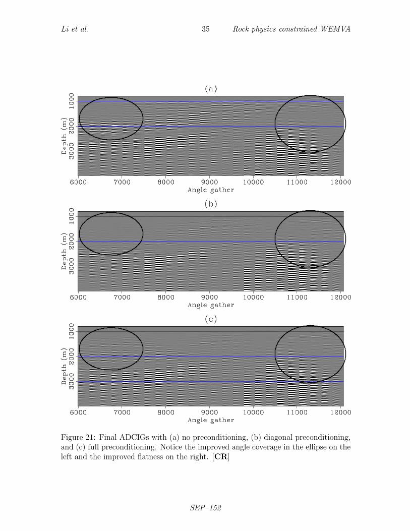
Figure 21 shows the comparison of the final ADCIGs with different preconditioningschemes. Compared with the initial ADCIGs in Figure 10(a), the inversion flattensthe angle domain events no matter which preconditioning scheme is applied. Thethree inversion tests give very similar results in the center of the section betweenx = 7.5 km and x = 10.5 km where the reflectors are illuminated by the data withrich angles. When the subsurface is less well illuminated by the data, for example inthe regions highlighted by the circles, the full preconditioning scheme produces flatterevents, stronger amplitudes, and higher angle coverage.

SEP–152

Li et al. 28 Rock physics constrained WEMVA

Figure 17: Inverted vertical velocity model after twenty iterations with (a) no precon-ditioning, (b) diagonal preconditioning and (c) full preconditioning. Panel (d) showsthe true vertical velocity model for comparison. [CR]

SEP–152

Li et al. 29 Rock physics constrained WEMVA

Figure 18: Inverted ε model after twenty iterations with (a) no preconditioning, (b)diagonal preconditioning and (c) full preconditioning. Panel (d) shows the true εmodel for comparison. [CR]

SEP–152

Li et al. 30 Rock physics constrained WEMVA

Figure 19: Inverted δ model after twenty iterations with (a) no preconditioning, (b)diagonal preconditioning and (c) full preconditioning. Panel (d) shows the true δmodel for comparison. [CR]

SEP–152

Li et al. 31 Rock physics constrained WEMVA

The WEMVA data fitting objective function can be evaluated at each imagingpoint. We compare the initial objective function map with the inverted objectivefunction map with different preconditioning schemes in Figure 22. The warmer colorindicates higher data fitting error, whereas the cooler color indicates lower data fittingerror. In the initial objective function map, the error is small in the shallow region(above 2.5 km) but it gets stronger with depth. As shown by the inverted objectivefunction map, the data fitting error has been significantly reduced in all three cases,especially in the regions between x = 1.5 km and x = 4 km and between x = 10 kmand x = 12 km.

To compare the objective function maps quantitatively (the visual comparison isdifficult due to their similarity), we subtract the objective function map in Figure22(d) from Figure 22(b) and plot the difference in Figure 23(a). Similarly, the dif-ference between Figures 22(d) and 22(c) is plotted in Figure 23(b). The region inred denotes the area where the inversion with full preconditioning fits the data betterthan the other two tests, and the region in blue denotes the opposite. The inversionwith full preconditioning does not guarantee a better fit for the data globally, but itdoes show better fits locally (Figure 22). Furthermore, the differences among differentpreconditioning schemes increase with depth as the data constraint becomes weakerwith depth.

Figure 24(a) plots the value of the data fitting objective function (sum of theobjective function map in Figure 22) as a function of iteration for three differentpreconditioning tests. The objective function value is normalized with respect tothe objective function value of the image migrated with the true models. All threeinversion tests reduce the objective function value to about 30% of the initial value.During the 20 iterations, the objective function values with the full covariance matrixare almost always the lowest among three tests; however, the differences among thethree objective values at each iteration are small. The curvature of the objectivefunction curves suggests that the inversion tests with diagonal or full preconditioninghave converged at iteration 20, whereas the inversion test without any preconditioningmay need more iterations to fully converge.

Figure 24(b) plots the normalized length of the gradient as a function of iterationfor three inversion tests. Although not guaranteed to be monotonically decreasing, thelength of the gradient should have a decreasing trend and should approach zero as theinversion converges, as shown by the curves with diagonal or full preconditioning. Onthe other hand, the gradient when no preconditioning is applied still has significantmagnitudes at the last few iterations. This is consistent with the objective functioncurve (magenta line in Figure 24(a)) that more iterations may be needed to improvethe convergence.

SEP–152

Li et al. 32 Rock physics constrained WEMVA

DISCUSSION

The nonlinear and underdetermined nature of the anisotropic model building problemleads to multiple VTI models that fit the same surface seismic data equally well. Thesemodels are referred to as equiprobable models (Yang et al., 2012; Osypov et al., 2008).The key element in this paper is the inclusion of the covariance matrix among theVTI parameters so that these equiprobable models can be differentiated from theprospective of the geological and lithological environment.

At first glance, one may have concerns about the reliability of the “extra” infor-mation from the preconditioning. However, our tests using different preconditioningon the synthetic example show that if the VTI parameters are well constrained bythe data in a certain region, different preconditioning schemes will not change thesolutions to those parameters when the convergence has been achieved in all theinversion tests. For those strongly constrained parameters, proper preconditioningsimply accelerates the convergence and enhances the resolution. The “extra” in-formation mostly affects the weakly constrained parameters, especially in the poorlyilluminated region. In these cases, the solutions to the model building problem can bedramatically different. It is possible that the rock physics model is inaccurate, whicheventually leads to erroneous VTI models in the less constrained region. However, theinverted VTI models are always consistent with the input rock physics information.Therefore, quick evaluation and modification of the models are possible when moreaccurate rock physics information is available.

As shown by the inversion results, even when the exact full preconditioning wasapplied in the tests, ambiguities among the VTI parameters cannot be completelyresolved. Two potential reasons may explain the residual ambiguity. First, the pre-conditioning scheme proposed in this paper utilizes the multivariate Gaussian distri-bution assumption among the VTI parameters. When the VTI parameters do notfollow the Gaussian distribution, the proposed formulation may not provide a suf-ficient description of the correlation among them. Moreover, the covariance matrixamong the VTI parameters is estimated based on the current VTI model and/or aprevious lithological interpretation. The conditional probability distribution mighthave been changed as the inversion updates the VTI parameters. Therefore, reevalu-ation of the covariance matrix might be necessary after a few nonlinear iterations tobetter mitigate the ambiguities.

SEP–152

Liet

al.33

Rock

physicscon

strained

WEM

VA

Figure 20: Final stacked images with (a) no preconditioning, (b) diagonal preconditioning, and (c) full preconditioning. Panel(d) shows the true stacked image. [CR]

SEP–152

Li et al. 34 Rock physics constrained WEMVA

CONCLUSION

This paper presents a preconditioned anisotropic WEMVA scheme to better con-strain the anisotropic model building process. The proposed preconditioning methodincludes lithological information in order to guide the inversion towards a plausiblegeological and rock physics solution. Numerical examples on a 2-D synthetic datasetshow that when proper preconditioning is applied during inversion, the inversionachieves the best resolution from the first iteration. By utilizing the cross-varianceamong the VTI parameters, the inversion also correctly resolves the less constrainedanisotropic parameter. Therefore, a properly preconditioned WEMVA inversion pro-vides a reliable tool for anisotropic model building.

ACKNOWLEDGEMENTS

The author thanks BP for providing the synthetic anisotropic model.

REFERENCES

Bachrach, R., 2010a, Applications of deterministic and stochastic rock physics mod-eling to anisotropic velocity model building: SEG Expanded Abstracts, 29, 2436–2440.

——–, 2010b, Elastic and resistivity anisotropy of compacting shale: Joint effectivemedium modeling and field observations: SEG Expanded Abstracts, 29, 2580–2584.

Bachrach, R., Y. K. Liu, M. Woodward, O. Zradrova, Y. Yang, and K. Osypov, 2011,Anisotropic velocity model building using rock physics: Comparison of compactiontrends and check-shot-derived anisotropy in the gulf of mexico: SEG ExpandedAbstract, 30, 207–211.

Bakulin, A., M. Woodward, D. Nichols, K. Osypov, and O. Zdraveva, 2009, Can wedistinguish TTI and VTI media?: SEG Expanded Abstracts, 28, 226–230.

——–, 2010a, Building tilted transversely isotropic depth models using localizedanisotropic tomography with well information: Geophysics, 75, 27–36.

——–, 2010b, Localized anisotropic tomography with well information in VTI media:Geophysics, 75, 37–45.

Bandyopadhyay, K., 2009, Seismic anisotropy: geological causes and its implications:PhD thesis, Stanford University.

Bear, L., T. Dickens, J. Krebs, J. Liu, and P. Traynin, 2005, Integrated velocity modelestimation for improved positioning with anisotropic PSDM: The Leading Edge,622–634.

Claerbout, J. F., 2009, Image estimation by example.Clapp, R., 2000, Geologically constrained migration velocity analysis: PhD thesis,

Stanford University.Dræge, A., M. Jakobsen, and T. A. Johansen, 2006, Rock physics modeling of shale

diagenesis: Petroleum Geoscience, 12, 49–57.

SEP–152

Li et al. 35 Rock physics constrained WEMVA

Figure 21: Final ADCIGs with (a) no preconditioning, (b) diagonal preconditioning,and (c) full preconditioning. Notice the improved angle coverage in the ellipse on theleft and the improved flatness on the right. [CR]

SEP–152

Li et al. 36 Rock physics constrained WEMVA

Figure 22: Comparison of the initial objective function map (a), with the final objec-tive function map with (b) no preconditioning, (c) diagonal preconditioning, and (d)full preconditioning. [CR]

Figure 23: Differences between the objective function maps. (a) Difference betweenFigure 22(d) and 22(b). (b) Difference between Figure 22(d) and 22(c). [CR]

SEP–152

Li et al. 37 Rock physics constrained WEMVA

Figure 24: Objective function value of the data fitting goal in (a) and the size of thegradient in (b) as a function of the iteration. Blue line: no preconditioning; red line:diagonal preconditioning; magenta line: full preconditioning. [CR]

Hornby, B., D. Miller, C. Esmersoy, and P. Christie, 1995, Ultrasonic-to-seismic mea-surements of shale anisotropy in a North Sea well: SEG Expanded Abstracts, 14,17–21.

Li, Y. and B. Biondi, 2011, Migration velocity analysis for anisotropic models: SEGExpanded Abstract, 30, 201–206.

Li, Y., D. Nichols, K. Osypov, and R. Bachrach, 2011, Anisotropic tomography usingrock physics contraints: 73rd EAGE Conference & Exhibition.

Li, Y. E., B. Biondi, R. Clapp, and D. Nichols, 2013, Wave equation migration velocityanalysis for VTI models: SEP-Report, 150, 157–168.

Li, Y. E., R. Clapp, B. Biondi, and D. Nichols, 2014, Rock physics constrainedanisotropic WEMVA: Part II - Field data test : SEP-Report, 152, 105–128.

Osypov, K., D. Nichols, M. Woodward, O. Zdraveva, and C. E. Yarman, 2008, Un-certainty and resolution analysis for anisotropy tomography using iterative eigen-decomposition: SEG Expanded Abstracts, 27, 3244–3249.

Sayers, C., 2004, Seismic anisotropy of shales: What determines the sign of Thomsen’sdelta parameter?: SEG Expanded Abstracts, 23, 103–106.

——–, 2010, The effect of anisotropy on the Young’s moduli and Poisson’s ratios ofshales: SEG Expanded Abstracts, 29, 2606–2611.

Tarantola, A., 1984, Inversion of seismic reflection data in the acoustic approximation:Geophysics, 49, 1259–1266.

Woodward, M. J., D. Nichols, O. Zdraveva, P. Whitfield, and T. Johns, 2008, Adecade of tomography: Geophysics, 73, VE5–VE11.

Yang, Y., K. Osypov, R. Bachrach, M. Woodward, O. Zdraveva, Y. Liu, A. Fournier,and Y. You, 2012, Anisotropic tomography and uncertainty analysis with rockphysics constraints: Green Canyon case study: SEG Expanded Abstract, 1–5.

SEP–152