Rodolphe Le Riche CNRS and Ecole des Mines de Saint-Etienne

1

Optimization with uncertaintiesMethods from the OMD projects

Rodolphe Le RicheCNRS and Ecole des Mines de Saint-Etienne

Uncertainty quantification for numerical model validation summer school, CEA Cadarache, June 2011

2

Outline of the talk

1. Introduction to optimization : uses, challenges.

2. Formulations of optimization problems with uncertainties

3. Noisy optimization

4. Kriging-based approaches (spatial statistics)

3

Goal of parametric numerical optimization

Ex : 15 bars truss, each bar chosen out of 10 profiles → 1015 possible trusses. How to choose ?Choose the position of the joints (continuous)→ How to search in R+,15 ?

4

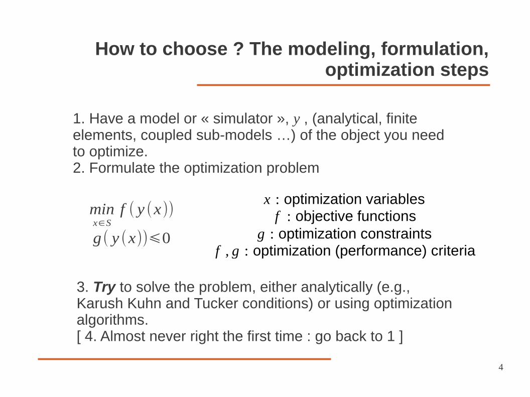
How to choose ? The modeling, formulation, optimization steps

1. Have a model or « simulator », y , (analytical, finite elements, coupled sub-models …) of the object you need to optimize.2. Formulate the optimization problem

minx∈S

f ( y (x))

g( y (x))⩽0

3. Try to solve the problem, either analytically (e.g., Karush Kuhn and Tucker conditions) or using optimization algorithms.[ 4. Almost never right the first time : go back to 1 ]

x : optimization variablesf : objective functions

g : optimization constraintsf , g : optimization (performance) criteria

5

Application example (1) : structural design

Maxx forward power

such that total power < powermax

parameterization = choice of x

simulation modely(x)

Luersen, M.A., Le Riche, R., Lemosse, D. and Le Maître, O.,A computationally efficient approach to swimming monofin optimization, SMO 2006

http://www.emse.fr/%7Eleriche/paper_monofin_SMO_2.pdf

6

Application example (2) : identification

x : material parametersMin

x distance( ymeasured , y(x) )

and similarly in supervised learning from data points (regression, classification, … ) : x = model parameters, f = data representation or classification error (+ regularization).

Silva, G., Le Riche, R., Molimard, J., Vautrin, A. and Galerne, C., Identification of material properties using FEMU : Application to the open hole tensile test, J. of Appl. Mech. and Mat. 2007

A. Rakotomamonjy, R. Le Riche, D.Gualandris and Z. Harchaoui, A comparison of statistical learning approaches for engine torque estimation, Control Engineering Practice, 2008.

7

Application examples (3)

Optimal control

x ≡ rudder_angle(t)f(x) ≡ time to goal

Modeling

in mechanicsx ≡ nodes displacementsf(x) ≡ total potential energyg(x) ≡ contact condition (non intrusion)

8

Optimization programs

An optimizer is an algorithm that iteratively proposes new x's based on past trials in order to approximate the solution to the optimization problem.

OSx(1)

x(1)f(x(1))

OSx(2)

x(t)f(x(t)) x(t+1)

Optimizer Simulator

x

f(y(x))

The cost of the optimization is the number of calls to the simulator y (usually = number of calls to f)

x(t+1) = Optimizer[x(1),f(x(1)) , … , x(t),f(x(t)) ]

If relevant , f → f and g , on other slides too.

9

Make can make optimizing difficult

local optima(expl. composites)

difficulties

Ill conditioning

Noise

Calculation cost of f

minx∈S⊂ℝn f x Goal :

Number of variables, n

10

Outline of the talk

1. Introduction to optimization



4. Kriging-based approaches

11

Formulations of optimization problems under uncertainties

G. Pujol, R. Le Riche, O. Roustant and X. Bay, L'incertitude en conception: formalisation, estimation, Chapter 3 of the book Optimisation Multidisciplinaire en Mécaniques : réduction de modèles, robustesse, fiabilité, réalisations logicielles, Hermes, 2009.

12

Formulation of optimization under uncertainty

The double (x,U) parameterization

x is a vector of deterministic optimization (controlled) variables.x in S, the search space.We introduce U, a vector of uncertain (random) parameters that affect the simulator y.

y(x) → y(x,U) , therefore f(x) → f(y(x,U)) = f(x,U) and g(x) → g(y(x,U)) = g(x,U)

U used to describe noise (as in identification with noise measurement) model error (epistemic uncertainty) uncertainties on the values of some parameters of y.

Ex : a +/- 1mm dispersion in the manufacturing of a car cylinder head can degrade its performance (g CO2/km) by +20% (worst case).

13

Formulation of optimization under uncertainty

The (x,U) parameterization is general

1. Noisy controlled variables

Expl : manufacturing tolerance U,

R = x1 + U

x = ( E(R), VAR(R) )

Two cases (which can be combined)

x1

L

R

x

L+U

2. Noise exogenous to the optimization variables

Expl : U random part load added to load L, x is a geometric dimension.

Expl : y finite element code, f volume of the structure, g upper bound on stresses.

tolerance class

nominalvalue

14

Formulation of optimization under uncertainties

(1) the noisy case

minx∈S

f (x ,U )

g(x ,U )⩽0

U random

Let's not do anything about the uncertainties, i.e., try to solve

It does not look good : gradients are not defined, what is the result of the optimization ? But sometimes there is no other choice. Ex : y expensive simulator with uncontrolled random numbers inside (like a Monte Carlo statistical estimation, numerical errors, measured input).

15

Formulation of optimization under uncertainties (2) an ideal series formulation

Replace the noisy optimization criteria by statistical measures

G(x) is the random event "all constraints are satisfied" , G(x) =∩

i{gi (x ,U )⩽0}

minx∈S

qαc (x) (conditional α -quantile)

such that P (G(x )) ⩾ 1−ε

where P ( f (x ,U )⩽qαc (x) | G(x)) = α

ε>0 , small

16

Formulation of optimization under uncertainties

(3) simplified formulations often seen in practice

For bad reasons (joint probabilities ignored) or good ones (simple numerical methods, lack of data, organisation issues), quantiles are often replaced by averages and variances, conditioning is neglected, constraints are handled independently :

such that P (G(x)) ⩾ 1−ε or P ( gi (x)⩽0 ) ⩾ 1−εi

where ε is the series system riskand εi is the i th failure mode risk

minx∈S

qα(x) or minx∈S

E ( f (x ,U )) and / or minx∈S

V ( f (x ,U ))

or minx∈S

E ( f (x ,U ))+r √V ( f (x ,U ))

where P ( f (x ,U )⩽qα ) = α and r>0

17

Scope of the presentation

The field of optimization under uncertainties is extremely active.

From here on, the presentation focuses on methods for optimization under uncertainties developped in the neighborhood of the speaker i.e.,

the French national projects OMD and OMD2 (where OMD stands for Optimisation MultiDisciplinaire, MDO).

In other words, many useful contributions are not presented.

Related books :

● OMD book : Multidisciplinary Design Optimization in Computational Mechanics, P. Breitkopf and R. Filomeno Coehlo Eds., Wiley/ISTE, 2010 ●A. Ben-Tal, L. El Ghaoui, A. Nemirowski, Robust Optimization, Princeton Univ. Press, 2009.● R. E. Melchers, Structural Reliability Analysis and Prediction, Wiley, 1999.● M. Lemaire, A. Chateauneuf, J.-C. Mitteau, Structural Reliability, Wiley, 2009.● J. C. Spall, Introduction to Stochastic Search and Optimization, Wiley, 2003.● A. J. Keane and P. B. Nair, Computational Approaches for Aerospace Design: The Pursuit of Excellence, Wiley, 2005.

18

Outline of the talk



3. Noisy optimization● The general CMA-ES● Improvements for noisy functions :

Mirrored sampling and sequential selectionAdding confidence to an ES


19

Continuous, unconstrained, noisy optimization

minx∈ℜn

f (x ,U ) and no control over U, seen as noise.

-2.0 -1.5 -1.0 -0.5 0.0 0.5 1.0 1.5 2.0-2.0

-1.5

-1.0

-0.5

0.0

0.5

1.0

1.5

2.0

-2.0 -1.5 -1.0 -0.5 0.0 0.5 1.0 1.5 2.0-2.0

-1.5

-1.0

-0.5

0.0

0.5

1.0

1.5

2.0

Expl : convergence of a quasi-Newton method with finite differences. A classical optimizer is sensitive to noise.

little noise more noise

f (x)=1

100 ∑i=1

100

∥x+ui∥2 ui ~ N (0, I 2) f (x)=∥x+ui∥

2

20

Noisy optimization

Evolutionary algorithms

Taking search decisions in probability is a way to handle the noise corrupting observed f values → use a stochastic optimizer, an evolution strategy (ES).Assumptions : none.

Initializations : x, f(x), m, C, tmax

.

While t < tmax

do,

Sample N(m,C) --> x'Calculate f(x') , t = t+1If f(x')<f(x), x = x' , f(x) = f(x') EndifUpdate m (e.g., m=x) and C

End while

A simple (1+1)-ES

%(Scilab code)x = m + grand(1,'mn',0,C)

« elitism »

21

Noisy optimization

Adapting the step size (C2) is important

(A. Auger et N. Hansen, 2008)

Above isotropic ES(1+1) : C = σ2 I , σ is the step size. With an optimal step size ( ≈ ║x║/ n ) on the sphere function, performance degrades only in O(n).

22

Noisy optimization

The population based CMA-ES

(N. Hansen et al., since 1996, now with A. Auger)

CMA-ES = Covariance Matrix Adaptation Evolution Strategy = optimization through sampling and updating of a multi-normal distribution.

A fully populated covariance matrix is build : pairwise variable interaction learned. Can adapt the step in any direction.

The state-of-the-art evolutionary / genetic optimizer for continuous variables.

23

Noisy optimization

flow-chart of CMA-ES

Initializations : m, C, tmax

, µ , λ

While t < tmax

do,

Sample N(m,C) --> x1,...,xλ

Calculate f(x1),...,f(xλ) , t = t+λRank : f(x1:λ),...,f(xλ:λ)Update m and C with the µ bests, x1:λ ,...,xµ:λ

End while

CMA-ES is a (non elitist) evolution strategy ES-(µ,λ) :

m et C are updated with ● the best steps (as opposed to points),● a time cumulation of these best steps.

24

Noisy optimization

CMA-ES : adapting C2 with good steps

x i= m yi

yi ∝ N 0,C i = 1, ... ,

(A. Auger et N. Hansen, 2008)

m∈S , C= I , ccov≈2/n2Initialization :

yw =1 ∑i=1

yi : m m yw

sampling

C 1−ccovCccov yw ywT

selection

rank 1 C update

update m

25

Noisy optimization

The state-of-the-art CMA-ES

(A. Auger and N. Hansen, A restart CMA evolution strategy with increasing population size, 2005)

Additional features :

● Steps weighting,

● Time cumulation of the steps.

● Simultaneous rank 1 and μ covariance adaptations.

● Use of a global scale factor, C → σ2 C .● Restarts with increasing population sizes (unless it is the 2010

version with mirrored sampling and sequential selection, see later)

Has been used up to n = 100 continuous variables.

yw = ∑i=1

w i y i :

26

Outline of the talk






27

Noisy optimization, improved optimizers

Mirrored sampling and sequential selection (1)

(1+1)-CMA-ES with restarts surprisingly good on some functions (including multimodal functions with local optima).

But « elitism » of (1+1)-ES bad for noisy functions : a lucky sample attracts the optimizer in a non-optimal region of the search space.

Question : how to design a fast local non-elistist ES ?

D. Brockhoff, A. Auger, N. Hansen, D. V. Arnold, and T. Hohm. Mirrored Sampling and Sequential Selection for Evolution Strategies, PPSN XI, 2010

A. Auger, D. Brockhoff, N. Hansen, Analysing the impact of mirrored sampling and sequential selection in elitist Evolution Strategies, FOGA 2011

28



Derandomization via mirrored sampling : one random vector generates two offsprings.Often good and bad in opposite directions.

Sequential selection : stop evaluation of new offsprings as soon as a solution better than the parent is found. Greedy !

Combine the two ideas : when an offspring is better than its parent, its symmetrical is worse (on convex level sets), and vice versa → evaluate in order m+y1 , m-y1 , m+y2 , m-y2 , … .

29



Results :

(1,4)-ES with mirroring and sequential selection faster than (1+1)-ES on sphere function.Theoretical result: Convergence Rate ES (1+1)=0.202 ,

Convergence Rate (1,4ms)=0.223 .

Implementation within CMA-ES, tested in BBOB'2010* (Black Box Optimization Benchmarking)Best performance among all algorithms tested so far on some functions of noisy testbed

* http://coco.gforge.inria.fr/bbob2010-downloads

30

Outline of the talk






31

Noisy optimization, ES with confidence

Adding confidence to an ES

Assumption : evaluations of f(x,u) can be repeated (even without control of u), f(x,u1), … , f(x,us)

Evolutionary optimizers are comparison based. We now compare empirical averages of f, therefore solve

minx E ( f (x ,U ))

D. Salazar, R. Le Riche, G. Pujol and X. Bay, An empirical study of the use of confidence levels in RBDO with Monte Carlo simulations, in Multidisciplinary Design Optimization in Computational Mechanics, Wiley/ISTE Pub., 2010.

Note : this can also be done with functions of f . For example, replace f(x,U) by its estimated e-th quantile (batching),

q (x ,U ) = f (x ,U ⌊ e×b ⌋) , f (x ,U 1)⩽…⩽f (x , U b)

32


Hypothesis testing

M 1,2 =1s ∑

i=1

s

f (x1,2 , ui) , V 1,2 =1

s−1 ∑i=1

s

( f (x1,2 , ui)−M 1,2 )2

Test : H0 the new point is better than the current one

HO , E ( f (x1 , U )) ⩾ E ( f (x2 ,U ))H1 , E ( f (x1 ,U )) < E ( f (x2 ,U ))

Statistic : Accept H0 if M 2−M 1

√V 1/s+V 2/ s< t 1−α ,

otherwise reject H0where t 1−α is the (1−α) 's quantile of a t -distributionα is the error rate at which H0 is wrongly rejected,

1-α

t1-α

α

1s∑i=1

s

f (x1 , ui)?

> , = , <1s

∑j=1

s

f (x2 , u j)

The decision to be made during the optimization, in the presence of noise, is (1 is current point , 2 the new point )

(same number of samples s to keep formula simple)

M and V are the empirical averages and variances,

33


ES and hypothesis testing

while cost < cost_max dox' = x(t) + σ N(0,I)calculate i.i.d. samples f(x',ui) , i = 1,scost = cost + sHypothesis testing : H0 , Ef(x',U) ≤ Ef(x(t),U) against H1 , Ef(x',U) > Ef(x(t),U)Reject H0 with error α ?

Yes : x(t+1) = x(t)No : x(t+1) = x'

t = t+1end

The simplest ES-(1+1) evolutionary optimizer improved by hypothesis testing.

● α allows to change continuously the behavior of the optimizer from exploratory (low α) to conservative (high α).● Three parameters, whose optimal values are coupled : σ , s , α

34


Test functions

F Qideal x = q90 f Q x , U

= q90 ∥xU∥2

F Hideal x = q90 f H x ,U

= q90 −1

∥x∥20.1U

decreasing signal / noise ratio as x → x* (=0)

increasing signal / noise ratio as x → x* (=0)

On unimodal noisy functions : test convergence speed in noise, not globality of the search

35


Parameters of the tests

σ : the optimizer step size (=0.05 to 4)nb : number of batches (=s). High noise when nb=2, little noise when nb=50.α : first type error rate where H0 is « the new point is better than the current one ».

α=0.1 : exploratory optimizerα=0.5 : traditional optimizer (no hypothesis testing)α=0.9 : conservative optimizer

( but also,n : number of variables, n=2 or 10. n=2 here, results generalize. Crude Monte Carlo (shown here) versus Latin Hypercube Sampling. Prefer LHS. )

Each optimization is started from {2}n, 500,000 calls to f long , and repeated 30 times.b = 20 (fixed, smallest number for a Gaussian percentile)

36


Number of MC simulations and step size

Lower bound on step sizes needs to increase with the noise (decreasing nb) to prevent comparison errors

nb = 50 : costly MC simulations, little noise

nb = 2 : cheap MC simulations, very noisy

Expl. on FH, traditional optimizer, the smallest step size (σ = 0.25)

overlined in red.

37


Number of MC simulations

Low MC number at the beginning (nb = 2), increase nb later to converge accurately (observed on F

Q and F

H).

Expl. on FQ, traditional optimizer, step size σ = 0.5 .

38


Traditional vs. exploratory optimizer

The exploratory optimizer (with HT, α=0.1) tends to diverge and never converges faster on FQ and FH → not useful on non-deceptive functions.

39


Conservative vs. traditional optimizer

Flat initial region (FH) with high probability of being mislead (nb = 2)

→ the conservative optimizer is initially the best. In all other tests made, traditional optimizer is better.

∥x−x*∥

40

Noisy optimization – Summary

minx f(x,U)

Use general stochastic (evolutionary) optimizers, which can be relatively robust to noise if properly tuned. Useful for optimizing statistical estimators which are noisy.

No control over the U's No spatial statistics (i.e. in S or S × U spaces), pointwise

approaches only.

Next : introduce spatial statistics to filter the noise → kriging based approaches.

41

Outline of the talk





42

Kriging : quick intro (1)

0 0 . 1 0 . 2 0 . 3 0 . 4 0 . 5 0 . 6 0 . 7 0 . 8 0 . 9 1- 1 . 5

- 1

- 0 . 5

0

0 . 5

1

1 . 5

x

f(x)

space x

f

black circles : observed values , f(x1), … , f(xt), with heterogeneous noise (intervals). Noise is Gaussian and independent at each point (nugget effect), variances δ

12 , … , δ

t2 .

Assume : the blue curves are possible underlying true functions.They are instances of stationary Gaussian processes Y(x) → fully characterized by their average μ and their covariance,

Cov (Y (x),Y (x ' ))=Fct (dist (x , x ' ))

43

Kriging : quick intro (2)

Kriging average : mK (x) = μ+cT(x)CΔ

−1(f−μ1)

Kriging variance : sK2 (x) = σ2−cT (x)CΔ

−1 c(x)

f (x) represented by Y t(x) = [ Y (x)∣ f (x1

),…, f (xt) ]

Y t (x) ∼ N (mK (x), sK2 (x)) (simple kriging)

c (x) = [Cov (Y (x),Y (x i)) ]i=1, t

CΔ = C+Δ

C = [Cov (Y (xi),Y (x j))] i , j

Δ = diag [δ12 , … , δt

2]

where

0 0 . 1 0 . 2 0 . 3 0 . 4 0 . 5 0 . 6 0 . 7 0 . 8 0 . 9 1- 1 . 5

- 1

- 0 . 5

0

0 . 5

1

1 . 5

x

f(x

)

space x

f

mK (x) mK (x)±sK (x)

44

Outline of the talk




4. Kriging-based approachesNo control on UWith control on U

45

No control on U.

The variance of the observations f(xi), ∆ , is

Kriging based optimization with uncertainties

No control on U

1. Estimated from the contextExpl : variance of a statistical estimator,

Quantile of f : cf. Le Riche et al., Gears design with shape uncertainties using

Monte Carlo simulations and kriging, SDM, AIAA-2009-2257.

2. Learned from dataBy maximizing the likelihood of the data (for ∆ and C parameters).Cf. Roustant, O. et al., DiceKriging, DiceOptim : two R packages for the analysis of computer experiments by kriging based metamodeling and optimization, HAL, 2010

Average f : V (f (x)) =1

s(s−1)∑i=1

s

(f (x ,ui)−f (x))2

46

The simplest approach.

Kriging based optimization with uncertainties, no control on U

Kriging prediction minimization

For t=1,tmax do,

Learn Yt(x) (mK and s

K2 ) from f(x1), … , f(xt)

xt+1 = minx m

K(x)

Calculate f(xt+1)t = t+1

End For

e.g., using CMA-ES because multimodal

(Krisp toolbox in Scilab)

But it may fail : the minimizer of mK

is at a data point which is not even a local optimum.

D. Jones, A taxonomy of global optimization methods based on response surfaces, JOGO, 2001.

47

A sampling criterion for global optimization without noise :


Expected Improvement criterion (1)

Improvement at x , I (x)=max( ymin−Y (x),0)

0 0 . 1 0 . 2 0 . 3 0 . 4 0 . 5 0 . 6 0 . 7 0 . 8 0 . 9 1

- 1

- 0 . 5

0

0 . 5

1

1 . 5

2n = 5

0 0 . 1 0 . 2 0 . 3 0 . 4 0 . 5 0 . 6 0 . 7 0 . 8 0 . 9 10

0 . 0 5

0 . 1

0 . 1 5

E I c r i t e r i o n

0 0 . 1 0 . 2 0 . 3 0 . 4 0 . 5 0 . 6 0 . 7 0 . 8 0 . 9 1

- 1

- 0 . 5

0

0 . 5

1

1 . 5

2n = 6

improvement instance, i

The expected improvement, EI(x) , can be analytically calculated.

EI increases when mK decreases and when

sK increases. EI(x) quantifies the

exploration-exploitation compromise of global optimization.

EI (x) = s(x) [ a(x)Φ ( a(x)) + ϕ ( a(x)) ] ,

a(x)=ymin−m(x)

s(x)

48

A sampling criterion for global optimization without noise :


Expected Improvement criterion

Improvement at x , I (x)=max( ymin−Y (x),0)

0 0 . 1 0 . 2 0 . 3 0 . 4 0 . 5 0 . 6 0 . 7 0 . 8 0 . 9 1

- 1

- 0 . 5

0

0 . 5

1

1 . 5

2n = 5

0 0 . 1 0 . 2 0 . 3 0 . 4 0 . 5 0 . 6 0 . 7 0 . 8 0 . 9 10

0 . 0 5

0 . 1

0 . 1 5

E I c r i t e r i o n

0 0 . 1 0 . 2 0 . 3 0 . 4 0 . 5 0 . 6 0 . 7 0 . 8 0 . 9 1

- 1

- 0 . 5

0

0 . 5

1

1 . 5

2n = 6

improvement instance, i

The expected improvement, EI(x) , can be analytically calculated. EI increases when m

K decreases and when s

K increases.

EI(x) quantifies the exploration-exploitation compromise of global optimization.

Next iterate : xt+1 = maxxEI(x)

Not suitable for noisy functions because the noise can make y

min too small and

create premature convergence around ymin

.

EGO (Efficient Global Optimization) algorithm, D. Jones, 1998 .

49

0 0 . 1 0 . 2 0 . 3 0 . 4 0 . 5 0 . 6 0 . 7 0 . 8 0 . 9 1- 1 . 5

- 1

- 0 . 5

0

0 . 5

1

1 . 5

x

f(x

)

x

f

Solution 1 : Add nugget effect and replace ymin

by the best observed mean (filters out noise in already sampled regions) :


EI for noisy functions

EInoisy (x)=E [max ( mini=1,t

mK (xi)−Y (x) , 0 )]

50


Expected Quantile Improvement

0 0 . 1 0 . 2 0 . 3 0 . 4 0 . 5 0 . 6 0 . 7 0 . 8 0 . 9 1

- 1 . 5

- 1

- 0 . 5

0

0 . 5

1

1 . 5

n = 4

0 0 . 1 0 . 2 0 . 3 0 . 4 0 . 5 0 . 6 0 . 7 0 . 8 0 . 9 10

0 . 0 5

0 . 1

0 . 1 5

0 . 2

E Q I c r i t e r i o n

0 0 . 1 0 . 2 0 . 3 0 . 4 0 . 5 0 . 6 0 . 7 0 . 8 0 . 9 1

- 1 . 5

- 1

- 0 . 5

0

0 . 5

1

1 . 5

n = 5

Solution 2 : Add nugget effect and use the expected quantile improvement. A conservative criterion (noise and spatial uncertainties are seen as risk rather than opportunities).

EQI (x) = E [max ( qmin−Q t+1(x) , 0 )]

qmin = mini=1,t

mK (xi)+α sK (xi

)

Q t+1(x) = mKt+1(x)+α sK

t+1(x)

mKt+1

(x) is a linear function of Y (x)

⇒ EQI (x) is known analytically

V. Picheny, D. Ginsbourger, Y. Richet, Optimization of noisy computer experiments with tunable precision, Technometrics, 2011.

51


Related work

E. Vazquez, J. Villemonteix, M. Sidorkiewicz and E. Walter, Global optimization based on noisy evaluations: an empirical study of two statistical approaches, 6th Int. Conf. on Inverse Problems in Engineering, 2010.

J. Bect, IAGO for global optimization with noisy evaluations, workshop on noisy kriging-based optimization (NKO), Bern, 2010.

52

Outline of the talk




4. Kriging-based approachesNo control on UWith control on U

53

Kriging based optimization with uncertainties

U control : uncertainty propagation

simulator

f x

uf(x,u)

x and u can be chosen before calling the simulator and calculating the objective function. This is the general case.

Optimization : loop on x

Estimation of the performance (average, std dev, percentile of f(x,U) ) : loop on u , Monte Carlo

Direct approaches to optimization with uncertainties have a double loop : propagate uncertainties on U, optimize on x.

Such a double loop is very costly (more than only propagating uncertainties or optimizing, which are already considered as costly) !

xu

f

54

Kriging based optimization with uncertainties, U controlled

(x,u) surrogate based approach

Assumptions : x and U controlled

Only one loop of f

(x,u) surrogate based approach

STAT [Y (x ,U )]

Y (x ,u)

f (x , u)(x , u)

Simulator

Optimizer

Direct approach

Multiplicative cost of two loops involving f

Monte Carlosimulations

f x ,uu

Simulator

Y (x )

STAT [ f (x ,U )]+εx

Optimizer of noisy functions

Y : surrogate model

55


A general Monte Carlo - kriging algorithm

Hereafter is an example of a typical surrogate-based (here kriging) algorithm for optimizing any statistical measure of f(x,u) (here the average).

Create initial DOE (Xt,Ut) and evaluate f there ;While stopping criterion is not met:

● Create kriging approximation Yt in the joint (x,u) space from f(Xt,Ut)

● Estimate the value of the statistical objective function from Monte Carlo simulations on the kriging average m

Yt.

Expl :

● Create kriging approximation Zt in x space from

● Maximize EIZ(x) to obtain the next simulation point → xt+1

ut+1 sampled from pdf of U

● Calculate simulator response at the next point, f(xt+1,ut+1). Update DOE and t

f̂ (xi) =

1s∑k=1

s

mKt(xi , uk

) , where uk i.i.d. from pdf of U

( xi , f̂ (xi))i=1,t

MC – kriging algorithm

only call to f !

56


Simultaneous optimization and sampling (1)

E [Y x ,U ]

Y x , u

f x ,u x , u

Simulator

1. Building internal representation of the objective (mean performance) by «integrated» kriging.

Optimizer

J. Janusevskis and R. Le Riche, Simultaneous kriging-based sampling for optimization and uncertainty propagation, ROADEF 2011 and HAL report.

Assumptions : x and U controlled, U normal. SolveY : kriging model

57


Integrated kriging (1)

: objective

objective

E[Z x ]

EU [ f x ,U ]

u

x

u approximation

integrate

: kriging approximation to deterministic

: integrated process approximation to

58


Integrated kriging (2)

-probability measure on U

The integrated process over U is defined as

Because it is a linear transformation of a Gaussian process, it is Gaussian, and fully described by its mean and covariance

Analytical expressions of mZ and cov

Z for Gaussian U's are given in

J. Janusevskis, R. Le Riche. Simultaneous kriging-based sampling for optimization and uncertainty propagation, HAL report: hal-00506957

59


Simultaneous optimization and sampling (2)

E [Y x ,U ]

Y x , u

f x ,u x , u

Simulator

1. Building internal representation of the objective (mean performance) by «projected» kriging.

Optimizer

2. Simultaneous sampling and optimization criterion for x and u(both needed by the simulator to calculate f)

60


EI on the integrated process (1)

Z is a process approximating the objective function

Optimize with an Expected Improvement criterion,

Optimize with an Expected Improvement criterion,

I Z(x)=max (zmin−Z (x),0) , but zmin not observed (in integrated space).⇒ Define zmin = min

x1,… , x t

E ( Z (x))

61



zmin

E[Z x ]

EU [ f x ,U ]

E[Z x ]STD [Z x]

62



x ok. What about u ? (which we need to call the simulator)

EU

63


Simultaneous optimization and sampling : method

xnext gives a region of interest from an optimization of the expected f point of view.

One simulation will be run to improve our knowledge of this region of interest → one choice of (x,u).

Choose (xt+1,ut+1) that provides the most information, i.e., which minimizes the variance of the integrated process at xnext

(no calculation details, cf. article. Note that VAR of a Gaussian process does not depend on f values but only on x's ).

64


Simultaneous optimization and sampling : expl.

EU

65


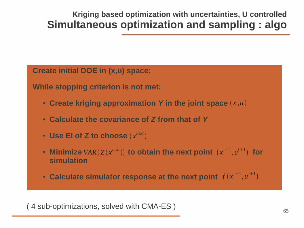
Simultaneous optimization and sampling : algo

( 4 sub-optimizations, solved with CMA-ES )

Create initial DOE in (x,u) space;

While stopping criterion is not met:

● Create kriging approximation Y in the joint space

● Calculate the covariance of Z from that of Y

● Use EI of Z to choose

● Minimize to obtain the next point for simulation

● Calculate simulator response at the next point

xnext

VAR Z xnext

f x t 1 , u t1

x ,u

x t 1 , ut 1

66


2D Expl, simultaneous optimization and sampling

DOE and E [Y x ,u]

EU [ f x ,U ]

VARΩ[Z (x)(ω)]

test function

E[Z x ]

EI Z x

67


1st iteration

DOE and E [Y x , u]

− x t 1 , u t1

− xnext ,

EU [ f x ,U ]

E[Z x ]

VAR [Z x]

EI Z x

68


2nd iteration

DOE and E [Y x ,u]

− x t 1 , u t1

− xnext ,

EU [ f x ,U ]

E[Z x ]

VAR [Z x]

EI Z x

69


3rd iteration

DOE and E [Y x ,u]

VAR [Z xnext] x , u

EU [ f x ,U ]

E[Z x ]

VAR [Z x]

EI Z x

70


5th iteration

DOE and E [Y x , u]

− x t 1 , u t1

− xnext ,

EU [ f x ,U ]

E[Z x ]

VAR [Z x]

EI Z x

71


17th iteration

DOE and E [Y x ,u]

EU [ f x ,U ] and E [Z x]

VAR [Z x]EI Z x

72


50th iteration

DOE and E [Y x ,u]

EU [ f x ,U ] and E [Z x]

VAR [Z x]EI Z x

73


Comparison tests

Compare « simultaneous opt and sampling » method to

1. A direct MC based approach : EGO based on MC simulations in f with fixed number of runs, s. Kriging with homogenous nugget to filter noise.

2. An MC-surrogate based approach : the MC-kriging algorithm.

74


Test functions

f (x)=−∑i=1

nsin(x i)[sin(ix i

2/π)]2

f x ,u=f x f u

Test cases based on Michalewicz function

nx=1 nu=1 μ=1.5 σ=0.2

nx=2 nu=2 μ=[1.5 , 2.1] σ=[0.2, 0.2]

nx=3 nu=3 μ=[1.5 , 2.1 , 2] σ=[0.2 , 0.2 , 0.3]

2D:

4D:

6D:

75


Test results

6D Michalewicz test case, nx =3 , n

U =3 .

Initial DOE: RLHS , m=(nx+n

U)*5 = (3+3)*5 = 30;

10 runs for every method.

Simult. opt & sampl.

MC-kriging

EGO + MC on f , s=3 , 5 , 10

76

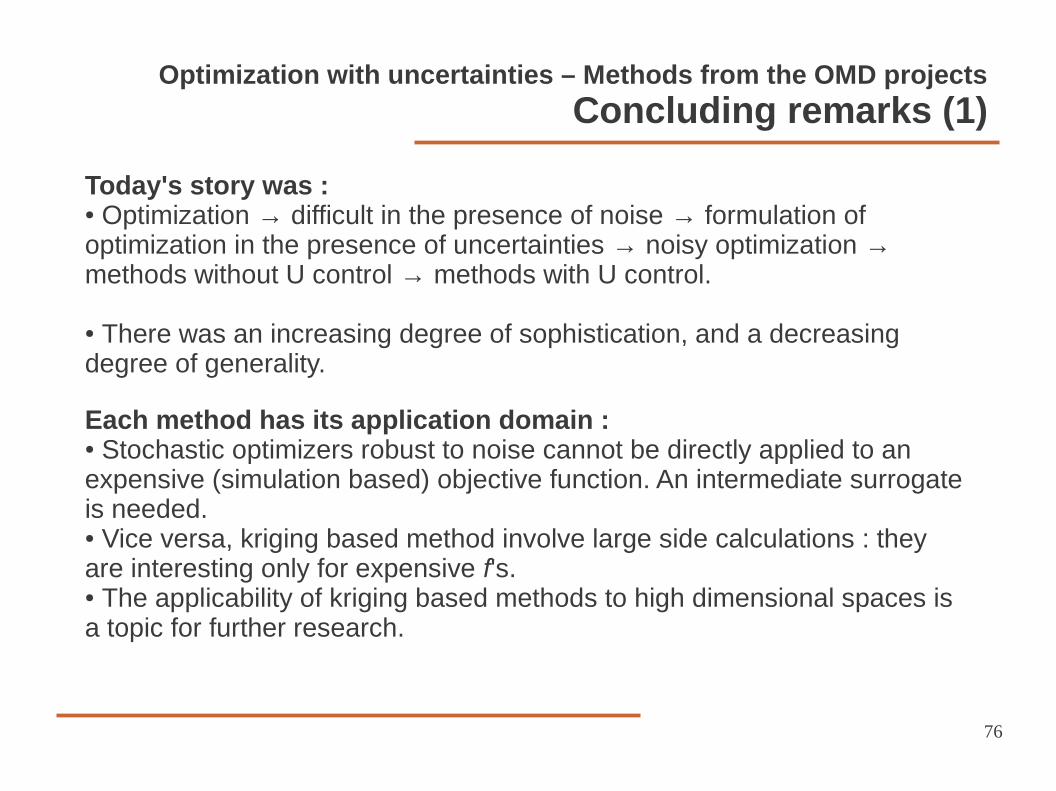
Optimization with uncertainties – Methods from the OMD projects

Concluding remarks (1)

Today's story was :● Optimization → difficult in the presence of noise → formulation of optimization in the presence of uncertainties → noisy optimization → methods without U control → methods with U control.

● There was an increasing degree of sophistication, and a decreasing degree of generality.

Each method has its application domain : ● Stochastic optimizers robust to noise cannot be directly applied to an expensive (simulation based) objective function. An intermediate surrogate is needed.● Vice versa, kriging based method involve large side calculations : they are interesting only for expensive f's.● The applicability of kriging based methods to high dimensional spaces is a topic for further research.

77

Optimization with uncertainties – Methods from the OMD projects

Concluding remarks (2)

The following methods within OMD projects were not discussed :

Method of moments ● R. Duvigneau, M. Martinelli, P. Chandrashekarappa, Uncertainty Quantification for Robust Design, Multidisciplinary Design Optimization in Computational Mechanics, Wiley, 2010.

FORM / SORM, optimal safety factor methods for reliability (constraints with uncertainties)● G. Kharmanda, A. El-Hami, E. Souza de Cursi, Reliability-Based Design Optimization, Multidisciplinary Design Optimization in Computational Mechanics, Wiley, 2010.● D. Villanueva, R. Le Riche, G. Picard, G., R.T. Haftka and B. Sankar, Decomposition of System Level Reliability-Based Design Optimization to Reduce the Number of Simulations, ASME 2011 conf.(IDETC).

(and of course a lot of the large litterature on the subject could not be covered).

Date post:	15-Feb-2022
Category:	Documents
Upload:	others
View:	2 times
Download:	0 times

Rodolphe Le Riche CNRS and Ecole des Mines de Saint-Etienne

Documents