ROMS Modeling for Marine Protected Area (MPA) Connectivity

Satoshi Mitarai, Dave Siegel, James Watson (UCSB)Charles Dong & Jim McWilliams (UCLA)

A biocomplexity project

“Flow, Fish & Fishing”

Coastal Environmental Quality Initiative (CEQI)

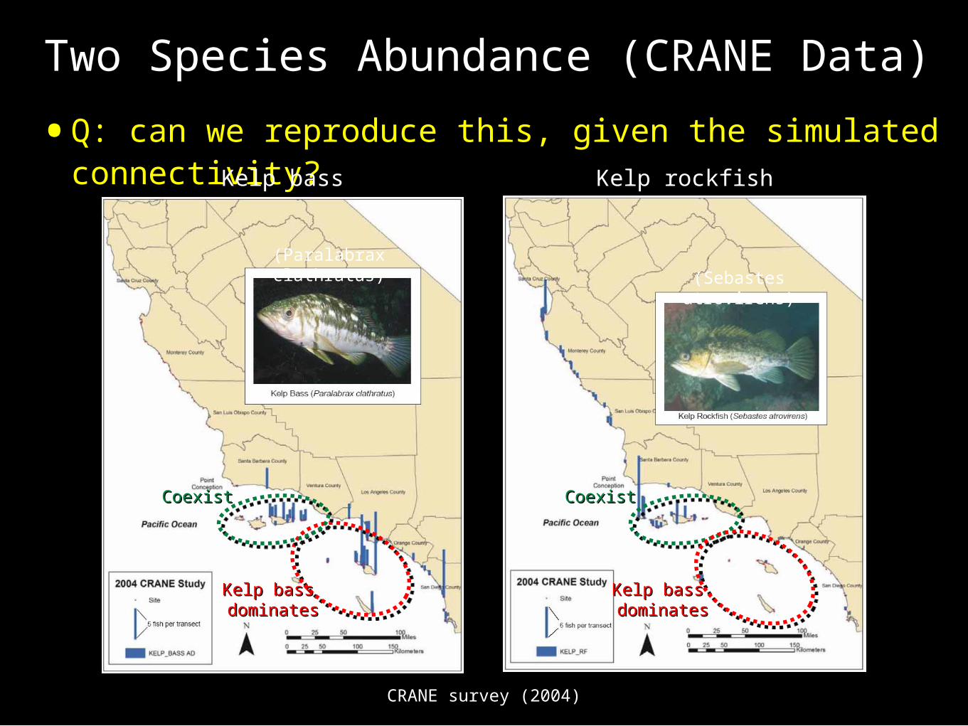
Marine Protected Areas (MPAs)

• To be implemented in Southern California Bight in 2009

Biomass DiversitySizeDensity

Per

cent

cha

nge 446%

166%

21%28%

30 cm 45 cm 60 cm

= 100,000 young

Science of marine reserve (2007)

Quantification of “Coastal Connectivity”

• Key info in designing a network of MPAs

= connectivity of nearshore sites via advection of water parcels

Rocky reefs in Southern California Bight

Rocky reefsRocky reefs

by Michael Robinson

Larval transport by coastal circulations

Advected 100’s km over months

Rocky reefs Rocky reefs

Good MPAcandidate

Good MPAcandidate

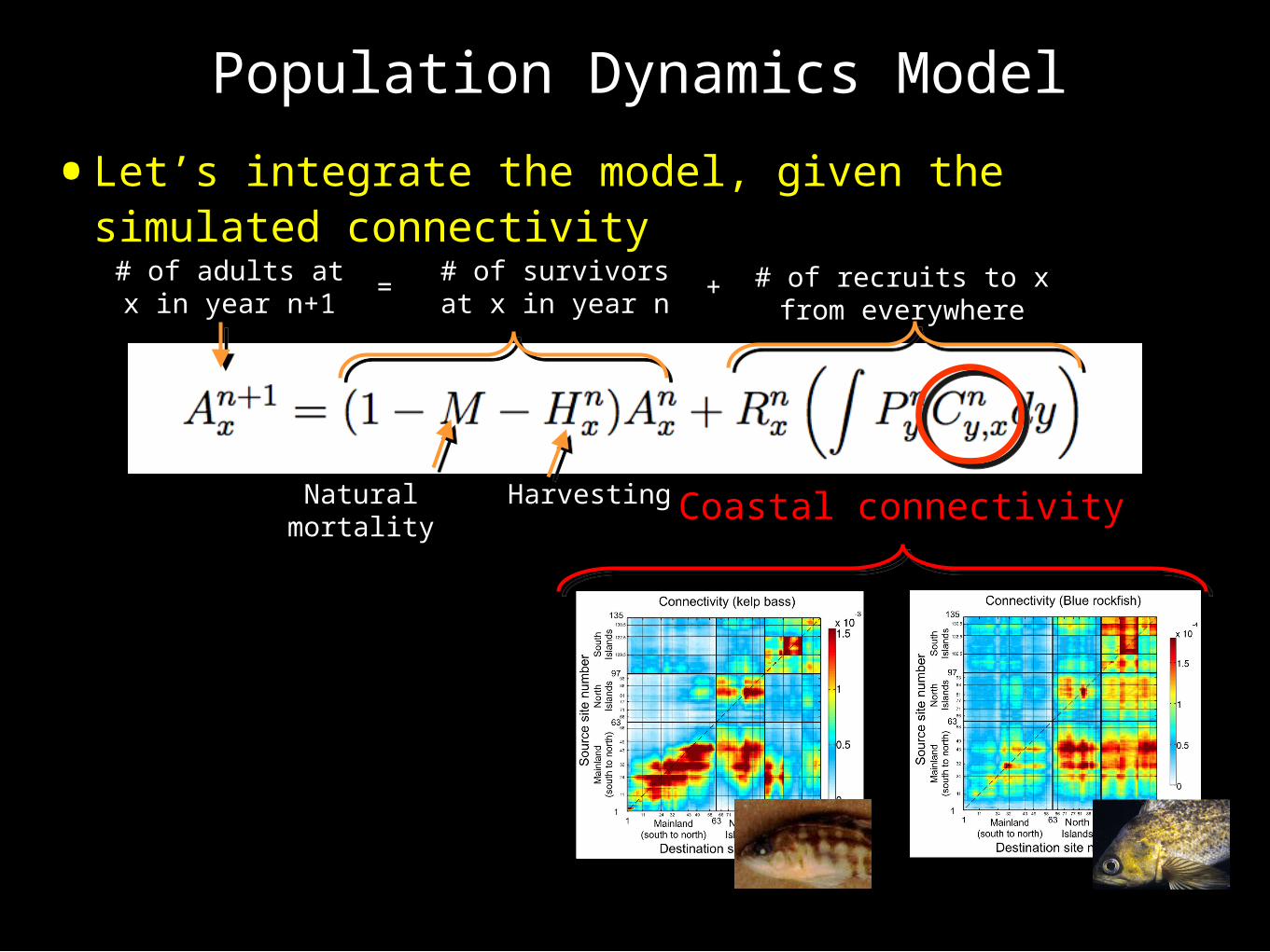
Natural mortality Harvesting

Population Dynamics Model

• Requires coastal connectivity info

# of adults at x in year n+1

# of recruits to x from everywhere

# of survivors at x in year n

= +

# of larvae produced at y

Fraction of water parcels transported to x

Recruitment success (%)

xy

Coastal connectivity

Goal of This Study

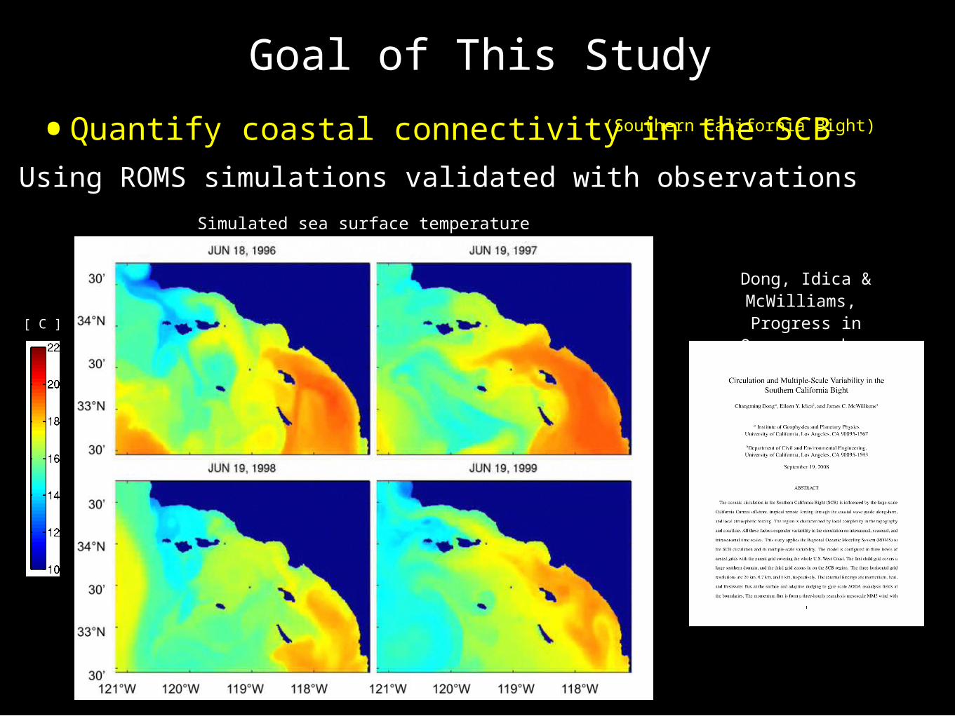
• Quantify coastal connectivity in the SCB

Using ROMS simulations validated with observations

[ C ]

Dong, Idica & McWilliams, Progress in Oceanography

(in revision)

Simulated sea surface temperature

(Southern California Bight)

Lagrangian PDF methods

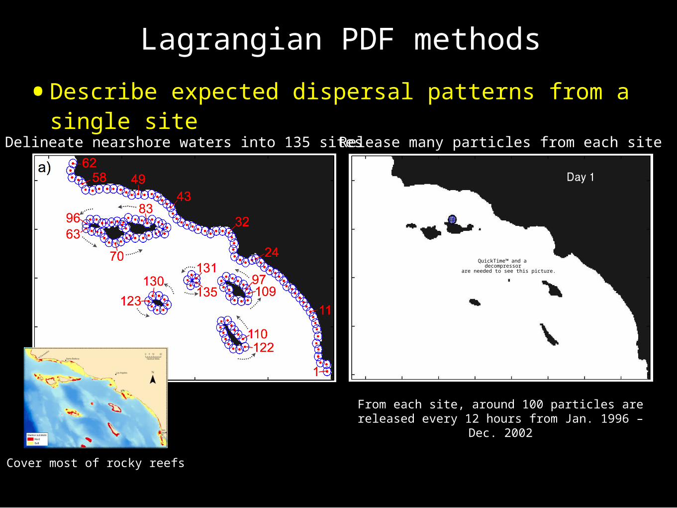
• Describe expected dispersal patterns from a single site

Delineate nearshore waters into 135 sites

Cover most of rocky reefs

Release many particles from each site

From each site, around 100 particles are released every 12 hours from Jan. 1996 – Dec. 2002

QuickTime™ and a decompressor

are needed to see this picture.

Sample Trajectories From Single Site

• Chaotic dominated by mesoscale eddy motions

Red dots: locations after 30 days

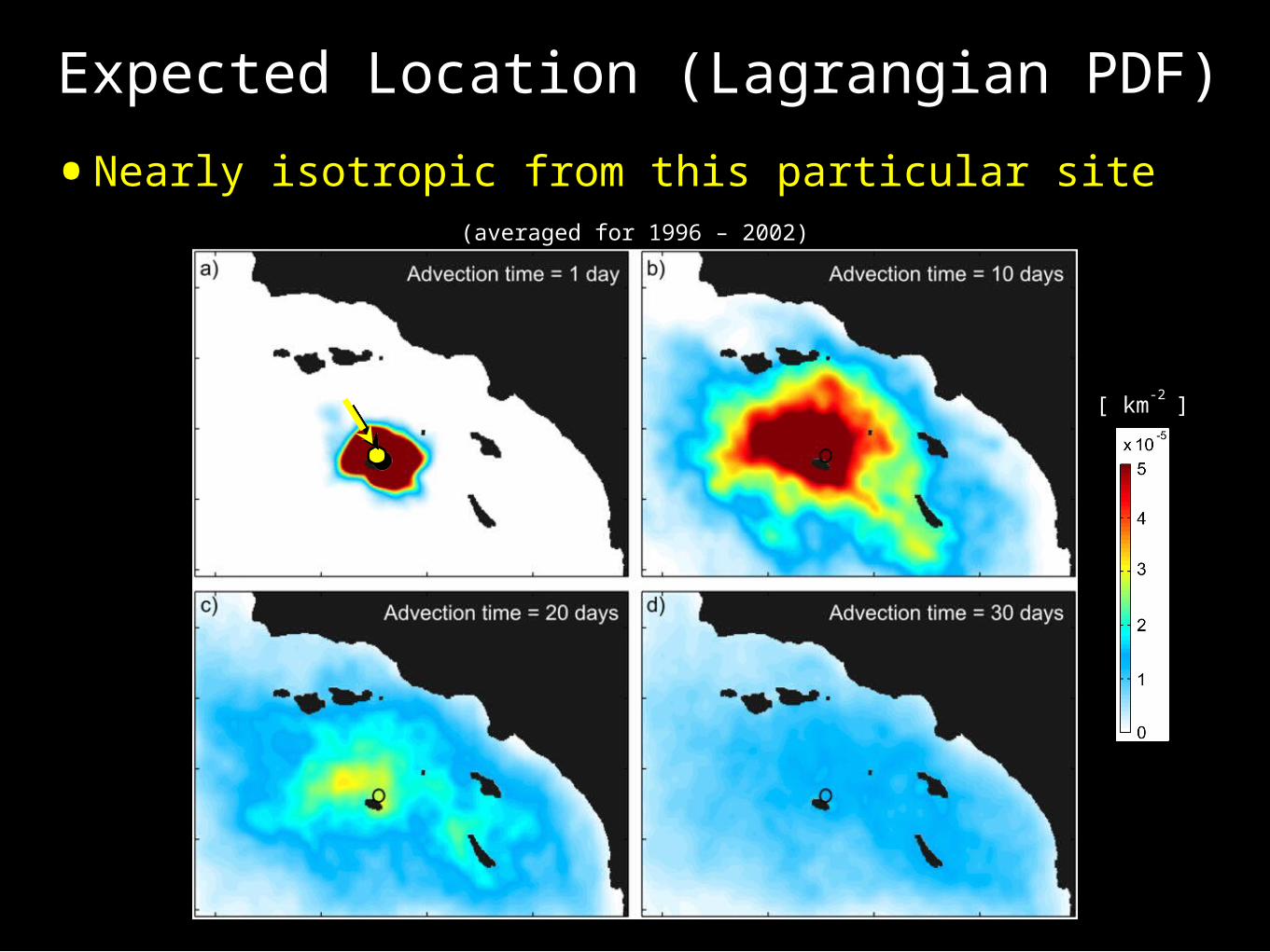
Expected Location (Lagrangian PDF)

• Nearly isotropic from this particular site

[ km ]-2

(averaged for 1996 – 2002)

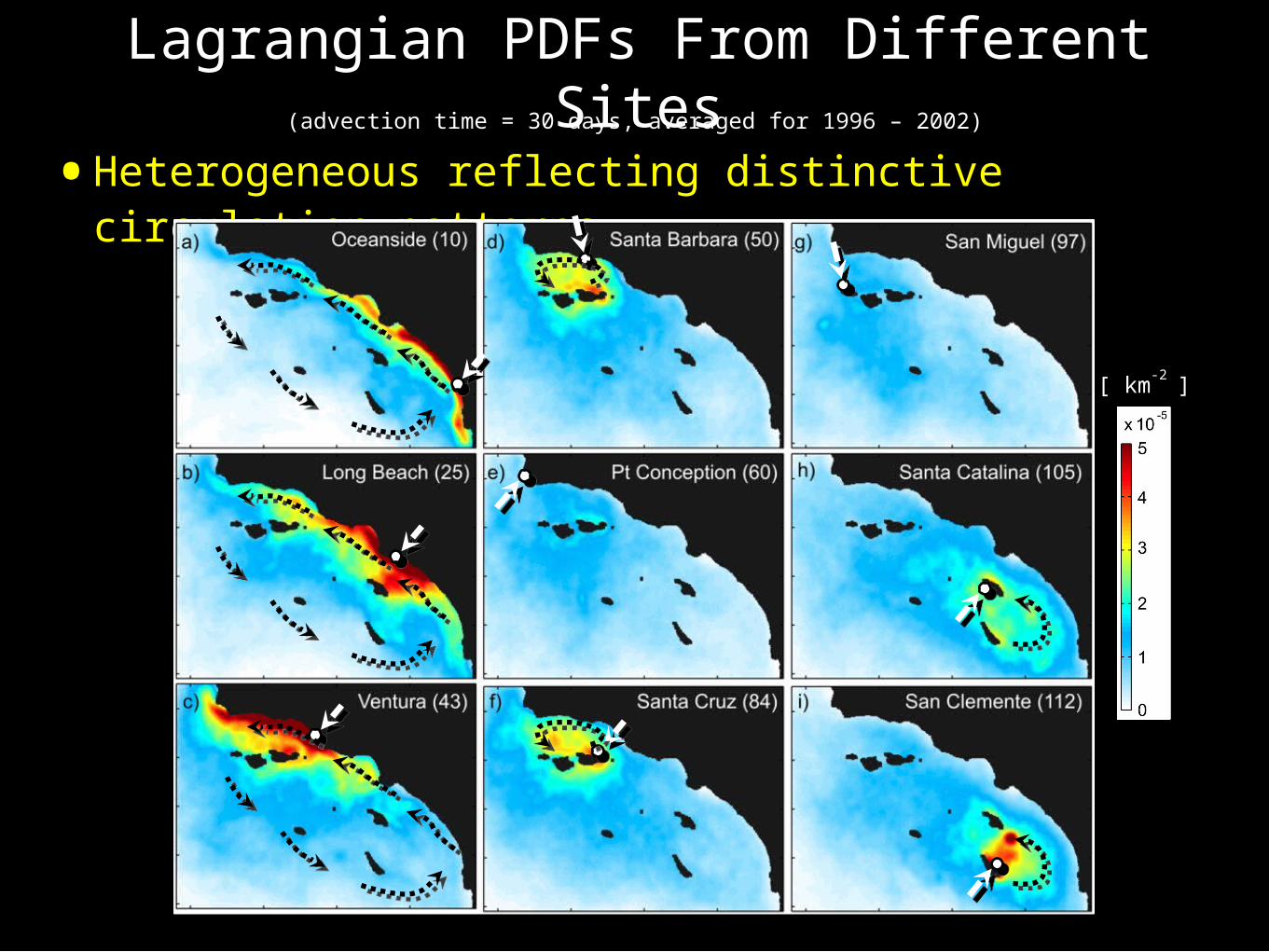
Lagrangian PDFs From Different Sites

• Heterogeneous reflecting distinctive circulation patterns(advection time = 30 days, averaged for 1996 – 2002)

[ km ]-2

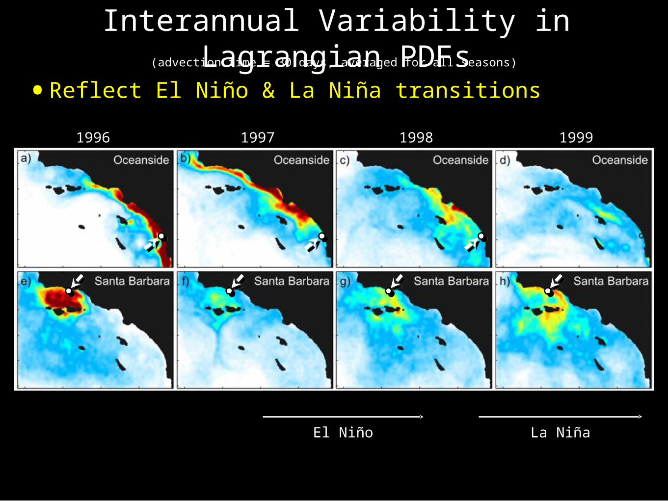
Seasonal Variability in Lagrangian PDFs

• Reflect seasonal variability in circulations(advection time = 30 days, averaged for 1996 – 2002)

Winter Spring Summer Autumn

Strong equatorward windReduced currentin SB Channel

Interannual Variability in Lagrangian PDFs

• Reflect El Niño & La Niña transitions

(advection time = 30 days, averaged for all seasons)

1996 1997 1998 1999

El Niño La Niña

Quantifying Coastal Connectivity

• Connectivity can be deduced from Lagrangian PDFs

Spawning: Apr – NovPlanktonic: 25 – 33 days

Kelp bass

Lagrangian PDF for kelp bass from site #43

Mainland to IslandsMainland to Islands

Islands to MainlandIslands to Mainland

Connectivity for Different Species

• Different due to different life histories

Spawning: Jan – MayPlanktonic: 60 – 180 days

Spawning: year aroundPlanktonic: 3 – 12 days

Potential Larval Source Locations

• Useful for MPA implementationWhere are larval sources?

Summation

Averaged for kelp bass, blue rockfish, Averaged for kelp bass, blue rockfish, lingcod, cabezon, canary rockfish & lingcod, cabezon, canary rockfish & red sea urchinred sea urchin

Santa Barbarax

Santa Cruz Santa Cruz IslandIslandSan MiguelSan Miguel

IslandIsland

Santa Barbara Santa Barbara IslandIsland

San Nicholas San Nicholas IslandIsland

x

Oceanside

San Miguel San Miguel IslandIsland

Anacapa Anacapa IslandIsland

San Clemente San Clemente IslandIsland

Santa CatalinaSanta CatalinaIslandIsland

Poor sources...Poor sources...

Summary

• Quantified connectivity in SCB using ROMS simulations

Lagrangian PDF method is employed

Connectivity is deduced from Lagrangian PDFs

• Potential larval sources are suggested

Some ongoing MPAs on Northern Islands are not really….

Mitarai, Siegel, Watson, Dong & McWilliams, JGR - Oceans (in review)

Questions

• How can we tell if the simulated connectivity is accurate?

Accurate enough for what?

To predict nearshore marine population dynamics

Distinctive biogeographic regions

Can we reproduce this?

Courtesy – Pete Raimondi

Two Species Abundance (CRANE Data)

• Q: can we reproduce this, given the simulated connectivity?Kelp bass Kelp rockfish

(Paralabrax clathratus)(Sebastes atrovirens)

CoexistCoexist

Kelp bass Kelp bass dominatesdominates

CoexistCoexist

Kelp bass Kelp bass dominatesdominates

CRANE survey (2004)

A Thought Experiment

• Two species population dynamics

Given the simulated connectivity matrices

Initialization (randomly seeded)

Species #2Species #2

Species #1Species #1

Spawning: Summer

Larval duration: 1 month

Life time: 20 years

#1. Kelp bass type

#2. Kelp rockfish type

Spawning: Winter

Larval duration: 2 months

Life time: 20 years

Population Dynamics Model

• Let’s integrate the model, given the simulated connectivity

# of adults at x in year n+1

# of recruits to x from everywhere

# of survivors at x in year n

= +

xy

Natural mortality Coastal connectivityHarvesting

Population Composition

• Shows reasonable agreement with CRANE data

Regardless of the initial condition

100 %species #1

100 %species #2

75 %species #1

75 %species #2

50-50

Kelp rockfish (#2)Kelp rockfish (#2)

Kelp bass (#1)Kelp bass (#1)

F1 / F2 = 1.1(when they coexist)

After reaches equilibrium

Kelp bass Kelp bass dominatesdominates

CoexistCoexist

Future Direction

• Integrate the framework into SCCOOS

Forecast dispersal, connectivity & population dynamics

Data assimilation?

• Clarify connectivity through boundaries

With Central Coast, across the international border

Important to address species invasion

• Lagrangian validation

Examine dispersal patterns against drifters & HF radar

(A part of Carter’s talk)

Thank you!