Page 1
Room acoustics: Idealized field and real field considerationsErnesto Accolti, and Fernando di Sciascio
Citation: Proc. Mtgs. Acoust. 31, 015003 (2017); doi: 10.1121/2.0000795View online: https://doi.org/10.1121/2.0000795View Table of Contents: http://asa.scitation.org/toc/pma/31/1Published by the Acoustical Society of America
Page 2
Volume 31 http://acousticalsociety.org/
174th Meeting of the Acoustical Society of AmericaNew Orleans, Louisiana
04-08 December 2017
Architectural Acoustics: Paper 2pAA4
Room acoustics: Idealized field and real field considerationsErnesto Accolti and Fernando di SciascioInstituto de Automatica, UNSJ - CONICET, San Juan, 5000, ARGENTINA; [email protected] ; [email protected]
How is an acoustically diffuse field defined? To what extent are the equations of diffuse field theory valid?These are the questions addressed in this presentation. The answers are explained through more general theories, in turn explained with figures. The starting point is the idealization of diffuse sound field, from where the basic calculation tools used in architectural acoustics are derived. Then, we go through the physical-mathematical models of wave theory and ray theory assuming diffuse field simplifications and analyze the scope of diffuse field models. Wave models and ray models are presented in a simple format with visual support and reference to the underlying mathematical models. The criteria used to define a diffuse field in frequency domain as well as in temporal domain are analyzed. Finally, we present a review of several state of the art tools used to address the real cases when diffuse field cannot be assumed.
Published by the Acoustical Society of America
© 2018 Acoustical Society of America. https://doi.org/10.1121/2.0000795Proceedings of Meetings on Acoustics, Vol. 31, 015003 (2018) Page 1
Page 3
1. INTRODUCTION The room acoustics discipline can be considered as a communication model in which the transmitter
are the sound sources, the medium is the air in the room as well as the borders of the room, and the receiver
are persons or eventually the microphones of measuring instruments, recording devices, electroacoustic
systems, or telecommunication systems. Formally, these communication models can be mathematically
formulated by the inhomogeneous Helmholtz wave equation. However, frequently accurate results are
achieved with approximated models based on sound rays.
The problem can be simplified when a diffuse field occurs. However, a diffuse field is an idealization
that can only be accepted when the results fall within a specified (or a reasonable) tolerance. Jeong (2016)
says that new measures are needed to quantify the degree of diffusion of reverberation chambers and that
subjective aspects of diffuseness have not been much investigated.
This article proposes a general method to define the scope of diffuse field models that should be applied
for a particular definition of the diffuse field according to each application. The proposed method is based
on time and frequency sliding windows, whose size depends on the application, that can be used to develop
a measure accounting for perceptive aspects, physical aspects, the position of the source and the receiver,
the sound content, etc.
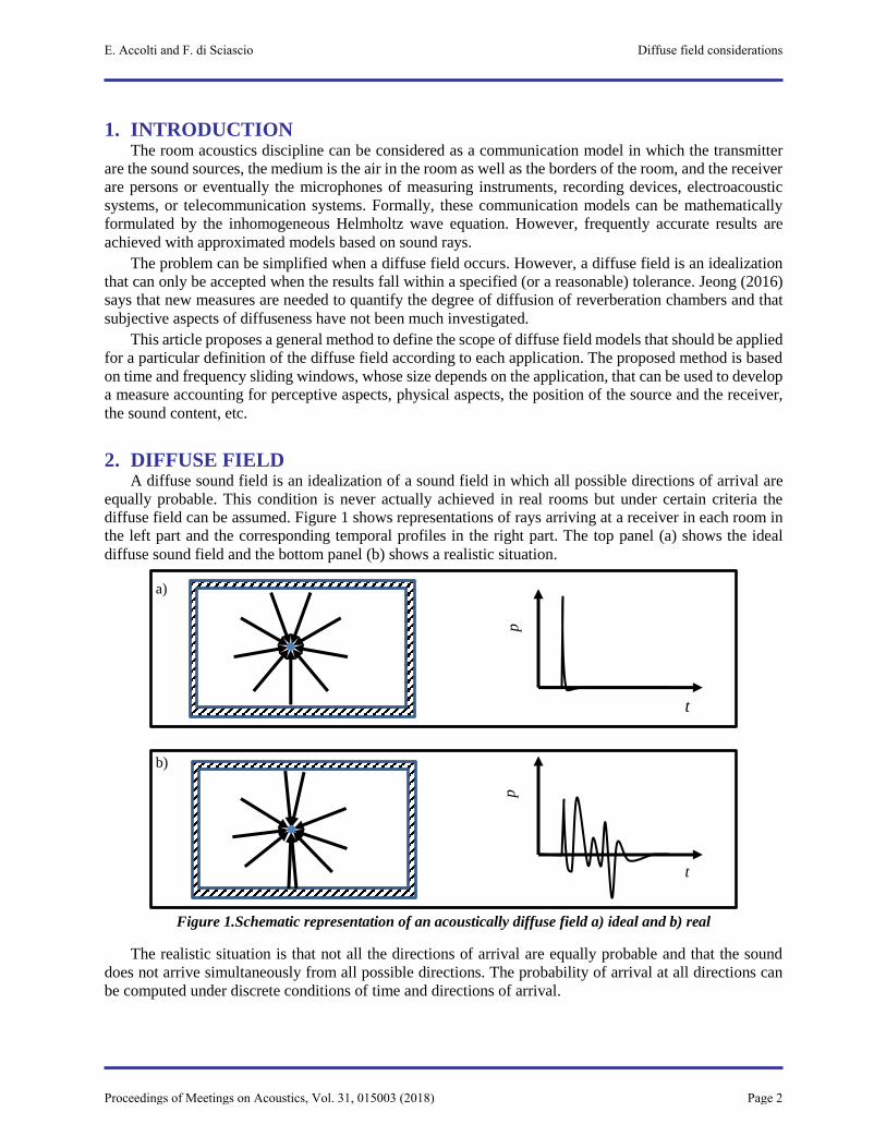
2. DIFFUSE FIELD A diffuse sound field is an idealization of a sound field in which all possible directions of arrival are
equally probable. This condition is never actually achieved in real rooms but under certain criteria the
diffuse field can be assumed. Figure 1 shows representations of rays arriving at a receiver in each room in
the left part and the corresponding temporal profiles in the right part. The top panel (a) shows the ideal
diffuse sound field and the bottom panel (b) shows a realistic situation.
Figure 1.Schematic representation of an acoustically diffuse field a) ideal and b) real
The realistic situation is that not all the directions of arrival are equally probable and that the sound
does not arrive simultaneously from all possible directions. The probability of arrival at all directions can
be computed under discrete conditions of time and directions of arrival.
t
p
t
p
a)
b)
E. Accolti and F. di Sciascio Diffuse field considerations
Proceedings of Meetings on Acoustics, Vol. 31, 015003 (2018) Page 2
Page 4
3. WAVE EQUATION MODELS The propagation theory of acoustic waves is a branch of physics based on a force diagram, continuity
of mass considerations, and the relations of an adiabatic process under an infinitesimal volume. The
adiabatic relation of sound pressure with variations of the density of the medium as an adiabatic process
can be modeled as a linear relation for a wide range of room acoustics applications. Considering a sound
source, these equations yield to the inhomogeneous Helmholtz equation
𝛻2𝑝 + 𝑘2𝑝 = −�̇� (1)
under border conditions
𝜁
𝜕𝑝
𝜕𝑛+ 𝑗𝑘𝑝 = 0 (2),
where p is the sound pressure, k is the wave number (k = ω/c), ζ is the specific acoustic impedance, and Ġ
is the velocity of mass increase per unit volume.
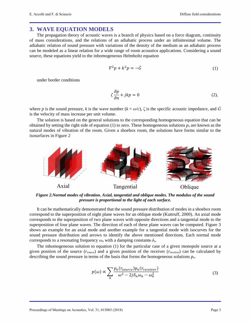
The solution is based on the general solutions to the corresponding homogeneous equation that can be
obtained by setting the right side of equation (1) to zero. These homogeneous solutions pn are known as the
natural modes of vibration of the room. Given a shoebox room, the solutions have forms similar to the
isosurfaces in Figure 2
Figure 2.Normal modes of vibration. Axial, tangential and oblique modes. The modulus of the sound
pressure is proportional to the light of each surface.
It can be mathematically demonstrated that the sound pressure distribution of modes in a shoebox room
correspond to the superposition of eight plane waves for an oblique mode (Kuttruff, 2000). An axial mode
corresponds to the superposition of two plane waves with opposite directions and a tangential mode to the
superposition of four plane waves. The direction of each of these plane waves can be computed. Figure 3
shows an example for an axial mode and another example for a tangential mode with isocurves for the
sound pressure distribution and arrows to identify the above mentioned directions. Each normal mode
corresponds to a resonating frequency ωn with a damping constants δn.
The inhomogeneous solution to equation (1) for the particular case of a given monopole source at a
given position of the source (rsource) and a given position of the receiver (rreceiver) can be calculated by
describing the sound pressure in terms of the basis that forms the homogeneous solutions pn.
𝑝(𝜔) ∝ ∑
𝑝𝑛(𝑟𝑠𝑜𝑢𝑟𝑐𝑒)𝑝𝑛(𝑟𝑟𝑒𝑐𝑒𝑖𝑣𝑒𝑟)
𝜔2 − 2𝑗𝛿𝑛𝜔𝑛 − 𝜔𝑛2
𝑛
(3)
Axial Tangential Oblique
E. Accolti and F. di Sciascio Diffuse field considerations
Proceedings of Meetings on Acoustics, Vol. 31, 015003 (2018) Page 3
Page 5
Figure 3. Normal modes composed of plane waves with given directions
Figure 4 shows a representation of equation 3 for a room of 7 m long, 5 m wide, and 3 m high with a
monopole source located at rsource = (1,3,1) and a receiver at rreceiver = (5,2,1.1). The blue line represents the
total frequency response and the black lines represent each term of equation (3) which in turn correspond
to the response of each mode.
Figure 4. Frequency response using wave theory for a shoebox room. The frequency is annotated in each
peak with red for axial modes, purple for tangential modes and light-blue for oblique modes
The first mode in figure 4 is an axial mode and so spreads in the room as a couple of plane waves with
opposite directions and of course it cannot be assumed as a diffuse field in which all directions of
propagation should be equally probable. Similar observations can be extended to each mode with two, four,
Tangential Mode (2,1,0)
Roo
m le
ngth
(m
)
Room long (m) Room long (m)
Axial Mode (1,0,0)
(1,0
,0)
25
Hz
(2,0
,0)
49
Hz
(0,1
,0)
34
Hz
(1,1
,0)
42
Hz
(0,0
,1)
69
Hz
(1,1
,1)
71
Hz
frequency (Hz)
So
und
le
ve
l (d
B)
Sliding
window
Sliding
window
E. Accolti and F. di Sciascio Diffuse field considerations
Proceedings of Meetings on Acoustics, Vol. 31, 015003 (2018) Page 4
Page 6
or eight plane waves. However, for higher frequencies the number of modes per unit of frequency
bandwidth increases and so does the number of possible directions of propagation per unit of frequency
bandwidth.
A frequency window can be defined and the probability of the direction of arrival of sound can be
estimated within this window. Then, the window can be slid on the frequency response of the room and the
probability of direction of arrival can be computed again. This procedure can be repeated and the directions
of arrival of sound energy will be more homogeneous as the frequency window slides to the high frequency
part of the frequency response.
An acceptable criterion of diffuse field can be developed for each application based in the possibility
for humans to hear a resonance, in the variance in measurements of reverberation time or of sound pressure
in different points of the room, or any other measurement ad-hoc to that application. The criterion should
define the size of the window, a measure of the probability of direction of arrival or another measure of
physical or perceptive parameters, and a tolerance value (or maximum allowable variance) for that measure.
4. RAY MODELS Ray theory in acoustics is derived from Snell’s law in optics. This is the simplest, most easily insightful
form of wave propagation theory. This theory estimates the sound field representing the emission from
sound sources as rays distributed in all directions that each source emits. Figure 5 shows that each ray has
its own direction.
Figure 5. Schematic representation of the ray theory model in a room
A receiver placed inside the room in figure 5 will receive rays from several directions. The impulse
response of the room can be calculated using an impulsive monopole point source and tracking the signal
at the receiver. Figure 6 shows a measured impulse response captured with a consumer recorder validated
for acoustical measurements (Miyara et al., 2010) and an omnidirectional condenser microphone. While
identifying the direct sound and the first reflections in Figure 6 is straightforward, identifying the late
reflections is hard because they are too close between them. A detailed review on current methods of
geometrical room acoustics modeling can be found in Savioja, L. and Svensson, 2015.
…
E. Accolti and F. di Sciascio Diffuse field considerations
Proceedings of Meetings on Acoustics, Vol. 31, 015003 (2018) Page 5
Page 7
Figure 6. Absolute value of impulse response measured for a concert hall (Accolti et al., 2017)
Each reflection and also the direct sound have well defined directions. Figure 7 shows the direction of
arrival of different rays. The time interval between reflection generally decrease for higher order reflections
that arrive later compared to direct sound and first reflections that correspond to low order reflections.
Figure 7. Propagation path of a direct sound ray, a first order reflection, and a forth order reflection.
A temporal window can be defined and the probability of the direction of arrival of sound can be
estimated in this window. Then the window can be slid on the impulse response of the room and the
probability of direction of arrival can be estimated again. This procedure can be repeated and the directions
of arrival of sound energy become more homogeneous as the time window slides to the late part of the
impulse response. An acceptable criterion of diffuse field can be developed for each application based on
the possibility for humans to hear an echo, a source location displacement, the variance in measurements
of reverberation time or sound pressure in different points of the room, or any other measurement ad-hoc
to the application. As in the frequency response case (in the section above) the criterion should define the
size of the window, a measure and a tolerance value for that measure.
5. CURRENT CRITERIA Criteria for both impulse response and frequency response are often used to identify the scope of diffuse
field methods and complement them with wave theory methods or ray acoustics methods. These existing
criteria are accurate for a great number of applications. However, depending on the application, more
accurate criteria can be developed based on time or frequency sliding windows.
A. FREQUENCY CRITERION
A well-known criterion is the Schroeder frequency (fc). This criterion states that at least three modes in
average are located in the bandwidth of one mode above fc for a room of volume V and reverberation time
T (Schroeder 1996).
0
0,2
0,4
0,6
0,8
1
0 25 50 75 100 125 150 175 200 225 250 275 300 325 350 375 400 425 450 475 500
(rela
tive u
nits׀(
p׀
time (ms)
direct sound
first reflections
E. Accolti and F. di Sciascio Diffuse field considerations
Proceedings of Meetings on Acoustics, Vol. 31, 015003 (2018) Page 6
Page 8
𝑓𝑐 = 2000√𝑇
𝑉 (4)
This criterion can also be described as a sliding window of variable size that should include at least
three modes in that window. Criteria depending on the number of modes are independent of the position of
the source and the receiver. Although these criteria are simple, some combinations of source-receiver could
not fulfil some expected considerations.
The frequency response was computed for two combinations of source-receiver positions by solving
the wave equation using the methods in Kuttruff (2000) for a shoebox room of 7 m long, 5 m wide, and 3 m
high. The 1/1 octave band response is computed as the accumulated sound energy in each band from the
solution of the wave equation. A second version of the 1/1 octave band response is computed using the
diffuse field equation
𝐿𝑝 = 𝐿𝑊 + 10 𝑙𝑜𝑔 (
𝑇
4𝜋𝑟2+
4 − 4 𝐴𝑆⁄
𝐴) (5)
where Lp is the sound pressure level, LW is the sound power level, T is the reverberation time, A is the total
sound absorption of the room, and S is the total area of the interior surfaces of the room. These three versions
of the frequency response are plotted together and the Schroeder frequency identified.
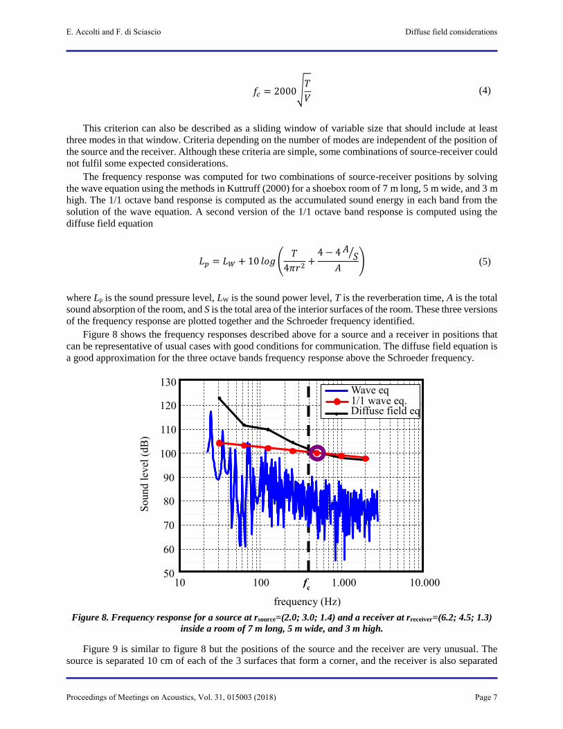
Figure 8 shows the frequency responses described above for a source and a receiver in positions that
can be representative of usual cases with good conditions for communication. The diffuse field equation is
a good approximation for the three octave bands frequency response above the Schroeder frequency.
Figure 8. Frequency response for a source at rsource=(2.0; 3.0; 1.4) and a receiver at rreceiver=(6.2; 4.5; 1.3)
inside a room of 7 m long, 5 m wide, and 3 m high.
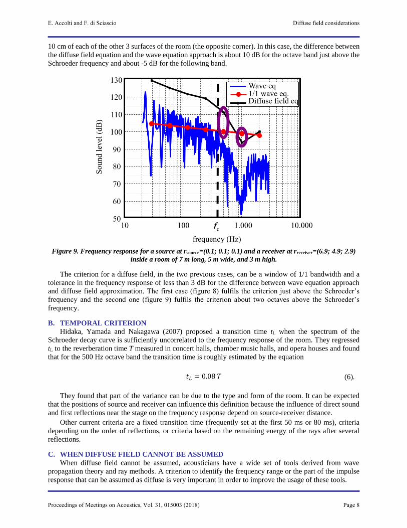
Figure 9 is similar to figure 8 but the positions of the source and the receiver are very unusual. The
source is separated 10 cm of each of the 3 surfaces that form a corner, and the receiver is also separated
10 100 1.000 10.000 50
60
70
80
90
100
110
120
130
frequency (Hz)
Soun
d l
evel
(dB
)
fc
Wave eq 1/1 wave eq. Diffuse field eq
E. Accolti and F. di Sciascio Diffuse field considerations
Proceedings of Meetings on Acoustics, Vol. 31, 015003 (2018) Page 7
Page 9
10 cm of each of the other 3 surfaces of the room (the opposite corner). In this case, the difference between
the diffuse field equation and the wave equation approach is about 10 dB for the octave band just above the
Schroeder frequency and about -5 dB for the following band.
Figure 9. Frequency response for a source at rsource=(0.1; 0.1; 0.1) and a receiver at rreceiver=(6.9; 4.9; 2.9)
inside a room of 7 m long, 5 m wide, and 3 m high.
The criterion for a diffuse field, in the two previous cases, can be a window of 1/1 bandwidth and a
tolerance in the frequency response of less than 3 dB for the difference between wave equation approach
and diffuse field approximation. The first case (figure 8) fulfils the criterion just above the Schroeder’s
frequency and the second one (figure 9) fulfils the criterion about two octaves above the Schroeder’s
frequency.
B. TEMPORAL CRITERION
Hidaka, Yamada and Nakagawa (2007) proposed a transition time tL when the spectrum of the
Schroeder decay curve is sufficiently uncorrelated to the frequency response of the room. They regressed
tL to the reverberation time T measured in concert halls, chamber music halls, and opera houses and found
that for the 500 Hz octave band the transition time is roughly estimated by the equation
𝑡𝐿 = 0.08 𝑇 (6).
They found that part of the variance can be due to the type and form of the room. It can be expected
that the positions of source and receiver can influence this definition because the influence of direct sound
and first reflections near the stage on the frequency response depend on source-receiver distance.
Other current criteria are a fixed transition time (frequently set at the first 50 ms or 80 ms), criteria
depending on the order of reflections, or criteria based on the remaining energy of the rays after several
reflections.
C. WHEN DIFFUSE FIELD CANNOT BE ASSUMED
When diffuse field cannot be assumed, acousticians have a wide set of tools derived from wave
propagation theory and ray methods. A criterion to identify the frequency range or the part of the impulse
response that can be assumed as diffuse is very important in order to improve the usage of these tools.
10 100 1.000 10.000 50
60
70
80
90
100
110
120
130
frequency (Hz)
Sound l
evel
(dB
)
fc
Wave eq 1/1 wave eq. Diffuse field eq
E. Accolti and F. di Sciascio Diffuse field considerations
Proceedings of Meetings on Acoustics, Vol. 31, 015003 (2018) Page 8
Page 10
Bolt (1946), Bonello (1981), and Cox et al. (2004) criteria for the distribution of normal modes are
good examples of tools to use in the frequency region where diffuse field cannot be assumed. These methods
allow to avoid modes that could be perceived or to identify compromising modes and modify them with
resonators or similar absorbers.
The non-diffuse field part of the impulse response is quite important because first reflections are
relevant aspects of the acoustic quality of several kind of rooms. Ray methods can help to design panels,
ceilings, or shells to influence on the first reflections (Beranek, 1992, Jurkiewicz et al., 2012, Miyara et al.,
2016). Ray methods are also used to avoid undesired effects such as echoes, direction of arrival mismatch,
or comb filtering.
D. EXISTING METHODS FOR FURTHER RESEARCH
The dependence of the sound sources and the content of the sound signals can be studied using
databases of audio recordings and methods that automatically generate audio signals based on parameters
such as the spectrum, the temporal characteristics, the signal to noise ratio, class of sounds events, etc.
These criteria can be generalized for certain applications by combining methods for automatic signal
generation and methods for room response modeling. Methods for automatic signal generation that combine
sound signals in order to obtain desired spectral and temporal characteristics were developed by Accolti
and Miyara (2015) and methods that can also obtain desired signal to noise ratios depending on frequency
were developed by Accolti et al. (2017b). The required measures can be obtained with questionnaires and
auralization techniques (Vorländer, 2008), ray acoustics models (Savioja and Svensson, 2015), or wave
equation models (Kuttruff, 2000) according to the application and in turn to the particular definition of the
diffuse field.
6. CONCLUSION This article proposes a general method to determine what parts of the room response are suitable for
considerations of a diffuse field. This method is based on a criterion that in turn depends on the application.
The method involves defining a measure, a tolerance value for that measure and the size of a sliding window
over which the measure is evaluated.
A case in which the octave band levels is required was studied and compared with the Schroeder’s
frequency criterion. Although the Schroeder’s frequency is a useful criterion, it was shown that this case
should be treated with other criteria.
These criteria can be used to define both frequency and time transitions. Currently available criteria are
good starting points but they can be improved for certain applications. The proposed method allows to
account for the effects of the position of the source and the receiver as well as for the specific goal of the
model that could be an acoustical physical measure as well as a sound perception measure.
Further investigation with audio signal processing and perception evaluations can use this method for
the development of simpler or adapted criteria for each application. The study of the influence of signal to
noise ratio, spectral and temporal issues of the signal could also be addressed with this method.
ACKNOWLEDGMENTS The authors acknowledge the support from the Acoustical Society of America, the Secretaría de Estado
de Ciencia Tecnología e Innovación de la Provincia de San Juan en Argentina (Secretary of State for
Science Technology and Innovation of the Province of San Juan, Argentina), the Consejo Nacional de
Investigaciones Científicas y Técnicas (National Scientic and Technical Research Council from Argentina),
and the Universidad Nacional de San Juan (National University of San Juan, Argentina).
REFERENCES Accolti, E., Alamino Naranjo, Y., Frank, A., Kuchen, E. Arballo, B. (2017) “The acoustics of the concert hall
Auditorio Juan Victoria from San Juan, Argentina” Proceedings of Meetings on Acoustics; vol. 28.
E. Accolti and F. di Sciascio Diffuse field considerations
Proceedings of Meetings on Acoustics, Vol. 31, 015003 (2018) Page 9
Page 11
Accolti, E., Miyara, F., di Sciascio, F. (2017b) “Generating sound stimuli with given emergence level and low
frequency content by mixing recordings” Acta Acustica united with Acustica 103(5), pp. 782–794.
Accolti, E., Miyara, F. (2015) “Method for generating realistic sound stimuli with given characteristics by controlled
combination of audio recordings” The Journal of the Acoustical Society of America, 137 (1), pp. EL85–EL90.
Beranek, L. L, (1992) “Concert hall acoustics—1992” The Journal of the Acoustical Society of America 1992, 1; 1–
39.
Bolt R., (1946) “Note on The Normal Frequency Statistics in Rectangular Rooms,” The Journal of the Acoustical
Society of America, 18, pp. 130–133.
Bonello, O. (1981) “A new criterion for the distribution of normal room modes”, Journal of the Audio Engineering
Society, 29, 597–606. Erratum, ibid., p. 905.
Cox, T. J., D’Antonio, P. and Davis, M.R. (2004) “Room sizing at low frequencies” Journal of the Audio Engineering
Society, 52: 640–651.
Hidaka T, Yamada Y, Nakagawa T. (2007) “A new definition of boundary point between early reflections and late
reverberation in room impulse responses” The Journal of the Acoustical Society of America 122(1):326–332.
Jeong, C. H. (2016) “Diffuse sound field: Challenges and misconceptions” Proceedings of the Proceedings of the 45th
International Congress on Noise Control Engineering, INTER-NOISE 2016, pp. 1015–1021.
Jurkiewicz, Y., Wulfrank, T, Kahle, E. (2012) “Architectural shape and early acoustic efficiency in concert halls” The
Journal of the Acoustical Society of America 132:3, 1253–1256
Kuttruff H. (2000) “Room acoustics” 4th Ed, Spon Press.
Miyara, F., Pasch, V., Accolti, E. (2017) “Analysis of lightweight acoustic reflectors” Proceedings of Meetings on
Acoustics, vol. 28.
Miyara, F., Accolti, E., Pasch, V., Cabanellas, S., Yanitelli, M., Miechi, P., Marengo Rodriguez, F.A., Mignini, E.
(2010) “Suitability of a consumer digital recorder for use in acoustical measurements” Proceedings of the 39th
International Congress on Noise Control Engineering 2010, INTER-NOISE 2010, 3, pp. 1811–1819.
Savioja, L. and Svensson, U. P. (2015) “Overview of geometrical room acoustic modeling techniques” The Journal
of the Acoustical Society of America 138:2, 708–730.
Schroeder, M. R. (1996) “The ‘‘Schroeder frequency’’ revisited” The Journal of the Acoustical Society of America
99, 3240–3241.
E. Accolti and F. di Sciascio Diffuse field considerations
Proceedings of Meetings on Acoustics, Vol. 31, 015003 (2018) Page 10