Rotation state evolution of retired geosynchronous ... · drives rotation state evolution of...

Rotation state evolution of retired geosynchronous satellites

Conor J. Benson and Daniel J. Scheeres

University of Colorado Boulder

429 UCB, Boulder, CO 80309

William H. Ryan and Eileen V. Ryan Magdalena Ridge Observatory, New Mexico Institute of Mining and Technology

101 East Road, Socorro, NM 87801

Nicholas Moskovitz Lowell Observatory

1400 W Mars Hill Road, Flagstaff, AZ, 86001

ABSTRACT

Non-periodic light curve rotation state analysis is conducted for the retired geosynchronous satellite GOES 8. This

particular satellite has been observed periodically at the Maui Research and Technology Center as well as

Magdalena Ridge and Lowell Observatories since 2013. To extract tumbling periods from the light curves, two-

dimensional Fourier series fits were used. Torque-free dynamics and the satellite’s known mass properties were then

leveraged to constrain the candidate periods. Finally, simulated light curves were generated using a representative

shape model for further validation. Analysis of the light curves suggests that GOES 8 transitioned from uniform

rotation in 2014 to continually evolving tumbling motion by 2016. These findings are consistent with previous

dynamical simulations and support the hypothesis that the Yarkovsky-O’Keefe-Radzievskii-Paddack (YORP) effect

drives rotation state evolution of retired geosynchronous satellites.

1. INTRODUCTION

With the growing value of geosynchronous orbit for communications and observation, understanding the motion of

defunct satellites in and near the geostationary belt is all the more important. Many of these satellites are known to

have fast or evolving spin states [1,2,3]. Better understanding of the mechanisms driving retired satellite rotation

state evolution promises a number of benefits. Knowledge of this motion will allow for the prediction of rapid spin

rates capable of material shedding or satellite break-up. In addition, this knowledge will yield more accurate

estimates for attitude dependent solar radiation forces for long-term orbit prediction. Finally, most proposed on-orbit

debris mitigation and servicing/recycling missions require physically restraining or grappling potentially tumbling,

non-cooperative target satellites. While designing and executing such missions, accurate predictions of the target’s

evolving rotation state will be invaluable.

Albuja et al. hypothesize that the observed evolution of some defunct satellites is largely driven by the Yarkovsky-

O’Keefe-Radzievskii-Paddack (YORP) effect, a phenomenon in which the absorption, reflection and delayed re-

emission of solar radiation generate torques on an orbiting body [4]. Through dynamical simulations, Albuja et al.

showed that YORP theory closely predicts the observed rotation period evolution of the retired GOES 8 and GOES

10 satellites [5]. Between December 2013 and July 2014, the observed rotation period of GOES 8 increased from

16.83 s to 75.66 s [2,3]. The Albuja et al. simulations also suggested a continued increase in GOES 8’s rotation

period resulting in a transition to non-principal-axis (tumbling) motion [5,6]. Photometric light curves of GOES 8

taken by Ryan & Ryan in September 2015 and February 2016 seemed to confirm this transition as the observations

did not exhibit clear periodicity [3,6]. Given these findings and the simulation results, Albuja et al. hypothesize that

GOES 8 and other retired satellites cycle between phases of uniform and tumbling motion due to the competing

influences of YORP and kinetic energy dissipation [6]. As a satellite’s spin rate approaches zero due to YORP, it

loses its angular momentum and begins to tumble. According to Albuja et al., the satellite then spins up

Copyright © 2017 Advanced Maui Optical and Space Surveillance Technologies Conference (AMOS) – www.amostech.com

preferentially about its axis of minimum inertia since this axis requires the minimum torque to accelerate. While

spinning up about this axis, energy dissipation starts to dominate. This eventually causes the satellite to return to

stable uniform rotation about the axis of maximum inertia. With all excess energy dissipated, YORP again becomes

the most dominant perturbation and the cycle starts over [6].

The following work will explore this cyclic hypothesis by analyzing several non-periodic optical light curves of

GOES 8 obtained between September 2015 and July 2016. Using frequency analysis and leveraging rigid body

dynamics, as well as shape and mass distribution information about GOES 8, plausible tumbling rotation states are

extracted from each light curve to gain insight into how the satellite is evolving.

2. OBSERVATIONS

GOES 8 has been observed several times at Magdalena Ridge Observatory (Socorro, NM) and Lowell Observatory

(Flagstaff, AZ) between September 2015 and July 2016. All Magdalena Ridge Observatory (MRO) observations

were taken using the observatory’s 2.4 m telescope fitted with an Andor iKon 936 CCD camera and Bessel VR

filter. Images were taken at a rate of 1-2 Hz with the exposure time adjusted for each arc based on satellite

brightness. Photometric data were obtained from the resulting images using the IRAF phot task, yielding

instrumental magnitudes only. Single data points with clear contamination from field stars were removed. Given the

fast sampling cadence and relatively large sidereal tracking rates, it was unlikely for a field star to contaminate

several consecutive images. So peak features with several or more data points were taken as satellite glints.

Reference [3] provides additional details about the instruments, data collection and reduction. The MRO light curves

are plotted in Fig. 1-2 along with the initial and final observer-satellite-sun phase angles for each arc. Fig. 1 shows

the 12 Sept 2015 GOES 8 light curve consisting of two segments separated by approximately 35 minutes. Upon

initial inspection, it is unclear if the satellite is tumbling given the earlier segment alone. The later segment on the

other hand clearly lacks defined periodicity.

Fig. 1. 12 Sept 2015 GOES 8 Light Curves

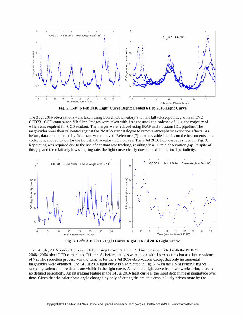
The 6 Feb 2016 light curve, plotted in Fig. 2, shows more structure than the previous one. On closer inspection

though, the aperiodic glint features and uneven peak spacing again suggest tumbling motion. This becomes more

apparent when the light curve is phase folded [2]. The smallest dispersion was found for a folded period of 13.64

min. Even for this best-fitting case, the folded light curve, plotted in Fig. 2, shows significant peak dispersion.

Previous GOES 8 observations show minimal dispersion for uniform rotation, even for large changes in solar phase

angle (~17°) [2].


Fig. 2. Left: 6 Feb 2016 Light Curve Right: Folded 6 Feb 2016 Light Curve

The 3 Jul 2016 observations were taken using Lowell Observatory’s 1.1 m Hall telescope fitted with an EV2

CCD231 CCD camera and VR filter. Images were taken with 1 s exposures at a cadence of 11 s, the majority of

which was required for CCD readout. The images were reduced using IRAF and a custom IDL pipeline. The

magnitudes were then calibrated against the 2MASS star catalogue to remove atmospheric extinction effects. As

before, data contaminated by field stars was removed. Reference [7] provides added details on the instruments, data

collection, and reduction for the Lowell Observatory light curves. The 3 Jul 2016 light curve is shown in Fig. 3.

Repointing was required due to the use of constant rate tracking, resulting in a ~5 min observation gap. In spite of

this gap and the relatively low sampling rate, the light curve clearly does not exhibit defined periodicity.

Fig. 3. Left: 3 Jul 2016 Light Curve Right: 14 Jul 2016 Light Curve

The 14 July, 2016 observations were taken using Lowell’s 1.8 m Perkins telescope fitted with the PRISM

2048×2064 pixel CCD camera and R filter. As before, images were taken with 1 s exposures but at a faster cadence

of 7 s. The reduction process was the same as for the 3 Jul 2016 observations except that only instrumental

magnitudes were obtained. The 14 Jul 2016 light curve is also plotted in Fig. 3. With the 1.8 m Perkins’ higher

sampling cadence, more details are visible in the light curve. As with the light curve from two weeks prior, there is

no defined periodicity. An interesting feature in the 14 Jul 2016 light curve is the rapid drop in mean magnitude over

time. Given that the solar phase angle changed by only 4° during the arc, this drop is likely driven more by the


satellite’s rotation than varying lighting geometry. When compared with the 6 Feb 2016 light curve, the two from

July have significantly higher frequencies, suggesting an increase in the satellite’s spin rate over this timespan.

3. METHODOLOGY

3.1 Tumbling Fundamental Periods

With the September 2015 – July 2016 GOES 8 light curves all demonstrating complex tumbling motion, methods

for extracting plausible tumbling rotation states from these light curves will now be discussed. Considering that

observed changes in GOES 8’s uniform rotation period occurred at much longer time scales than a typical

observation arc (<1 hr), it will be assumed that the satellite’s motion can be well-approximated by torque-free rigid

body dynamics for the duration of a given light curve. Under torque-free rigid body assumptions, the tumbling

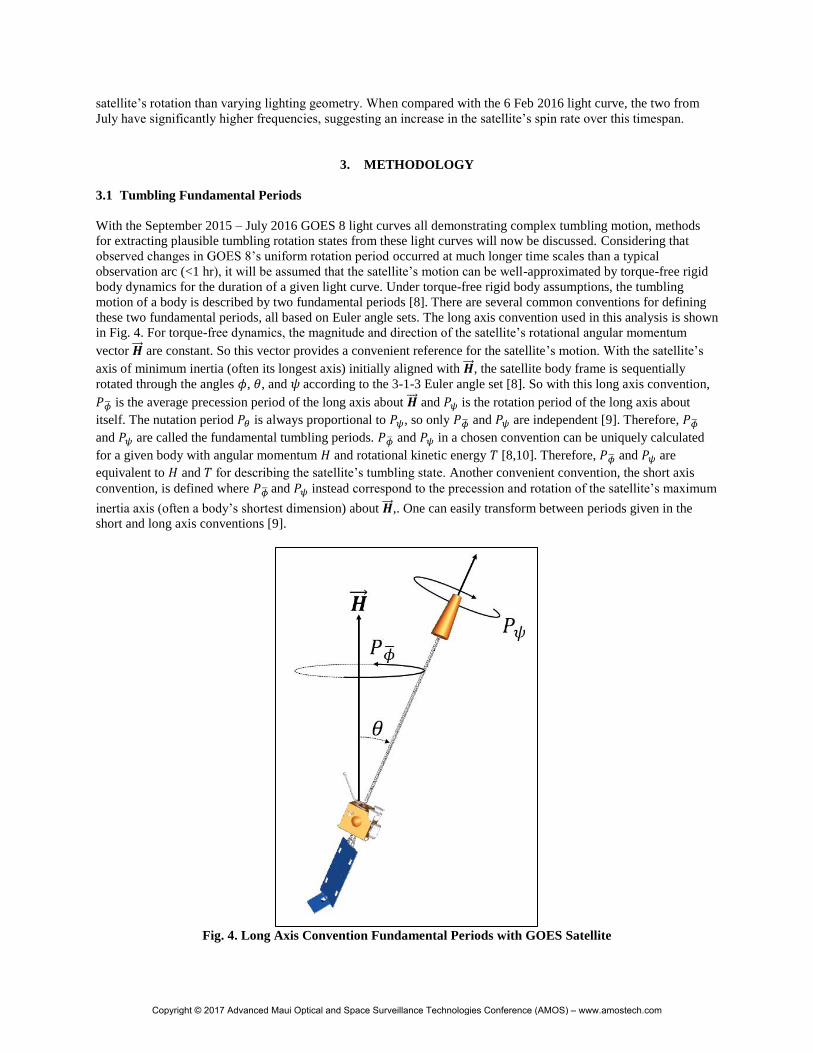
motion of a body is described by two fundamental periods [8]. There are several common conventions for defining

these two fundamental periods, all based on Euler angle sets. The long axis convention used in this analysis is shown

in Fig. 4. For torque-free dynamics, the magnitude and direction of the satellite’s rotational angular momentum

vector �⃗⃗⃗� are constant. So this vector provides a convenient reference for the satellite’s motion. With the satellite’s

axis of minimum inertia (often its longest axis) initially aligned with �⃗⃗⃗� , the satellite body frame is sequentially

rotated through the angles 𝜙, 𝜃, and 𝜓 according to the 3-1-3 Euler angle set [8]. So with this long axis convention,

𝑃�̅� is the average precession period of the long axis about �⃗⃗⃗� and 𝑃𝜓 is the rotation period of the long axis about

itself. The nutation period 𝑃𝜃 is always proportional to 𝑃𝜓, so only 𝑃�̅� and 𝑃𝜓 are independent [9]. Therefore, 𝑃�̅�

and 𝑃𝜓 are called the fundamental tumbling periods. 𝑃�̅� and 𝑃𝜓 in a chosen convention can be uniquely calculated

for a given body with angular momentum 𝐻 and rotational kinetic energy 𝑇 [8,10]. Therefore, 𝑃�̅� and 𝑃𝜓 are

equivalent to 𝐻 and 𝑇 for describing the satellite’s tumbling state. Another convenient convention, the short axis

convention, is defined where 𝑃�̅� and 𝑃𝜓 instead correspond to the precession and rotation of the satellite’s maximum

inertia axis (often a body’s shortest dimension) about �⃗⃗⃗� ,. One can easily transform between periods given in the

short and long axis conventions [9].

Fig. 4. Long Axis Convention Fundamental Periods with GOES Satellite


3.2 Two-Dimensional Fourier Series

Generally, the frequencies present in a tumbling light curve are linear combinations of the fundamental frequencies

𝑓�̅� = 1/𝑃�̅� and 𝑓𝜓 = 1/𝑃𝜓 [9,11,12]. Therefore the time-varying brightness 𝐵(𝑡) of a tumbling light curve can be

modeled using a two-dimensional Fourier series,

𝐵(𝑡) = 𝐶0 + ∑[𝐶𝑗0 cos 2𝜋𝑗𝑓1𝑡 + 𝑆𝑗0 sin 2𝜋𝑗𝑓2𝑡]

𝑚

𝑗=1

+ ∑ ∑ [𝐶𝑗𝑘 cos 2𝜋(𝑗𝑓1 + 𝑘𝑓2)𝑡 + 𝑆𝑗𝑘 sin 2𝜋(𝑗𝑓1 + 𝑘𝑓2)𝑡]

𝑚

𝑗=−𝑚

𝑚

𝑘=1

Here, 𝑓1 and 𝑓2 are the fundamental frequencies, 𝑚 is the Fourier series order, 𝐶0 is the mean light curve brightness,

and (𝐶𝑗𝑘, 𝑆𝑗𝑘) are the coefficients associated with each linear combination of 𝑓1 and 𝑓2 [12]. This Fourier series

model assumes that the brightness variation is driven solely by the satellite’s rotation with fixed lighting and

viewing geometry. Therefore, it will only approximate real satellite light curves since time-varying solar phase

angles and synodic vs. sidereal spin rates also influence the observed brightness variation.

To extract the fundamental periods from a tumbling light curve, one can search a grid of potential period pairs. For

each pair, a two-dimensional Fourier series of order 𝑚 is fit to the observations using a least squares method. The

goal is to find the period pair yielding the best fit to the observations (i.e. the lowest residual). There are a number of

issues with this approach though. First of all, several different period pairs often fit the light curve well. Also, the

fitting process provides no information about which of the two periods 𝑃1 = 1/𝑓1 and 𝑃2 = 1/𝑓2 correspond to 𝑃�̅�

and 𝑃𝜓. Finally, a given (𝑃�̅�, 𝑃𝜓) pair can describe both a long axis mode (LAM) and short axis mode (SAM)

tumbling state. For LAM states, �⃗⃗⃗� precesses about the axis of minimum inertia. For SAM states, �⃗⃗⃗� precesses about

the axis of maximum inertia [13]. Furthermore, being closer to uniform rotation about the maximum inertia axis

(minimum energy state), SAMs have lower energy than LAMs. Therefore, a satellite in LAM experiencing energy

dissipation will be driven through the SAM regime towards uniform rotation about the maximum inertia axis.

Returning to periods assignments, a (𝑃1,𝑃2) pair could correspond to any of four possible tumbling states.

3.3 Moment of Inertia Constraints

One way to constraint the possible periods is to leverage moment of inertia information about the satellite. Only

some (𝑃�̅�, 𝑃𝜓) pairs are physically possible for given moments of inertia [8,9,10,11]. If the satellite’s moments of

inertia are known, each of the four candidate period assignments can be tested for viability. Fortunately, GOES 8’s

end of life moments of inertia are known [5]:

[𝐼]𝐺𝑂𝐸𝑆 8 = [

𝐼𝑙 0 00 𝐼𝑖 00 0 𝐼𝑠

] = [980.5133 0 0

0 3440.9438 00 0 3561.0894

] 𝑘𝑔 𝑚2

Following the conventions described earlier, 𝐼𝑙 , 𝐼𝑖 , and 𝐼𝑠 are the satellite’s minimum, intermediate, and maximum

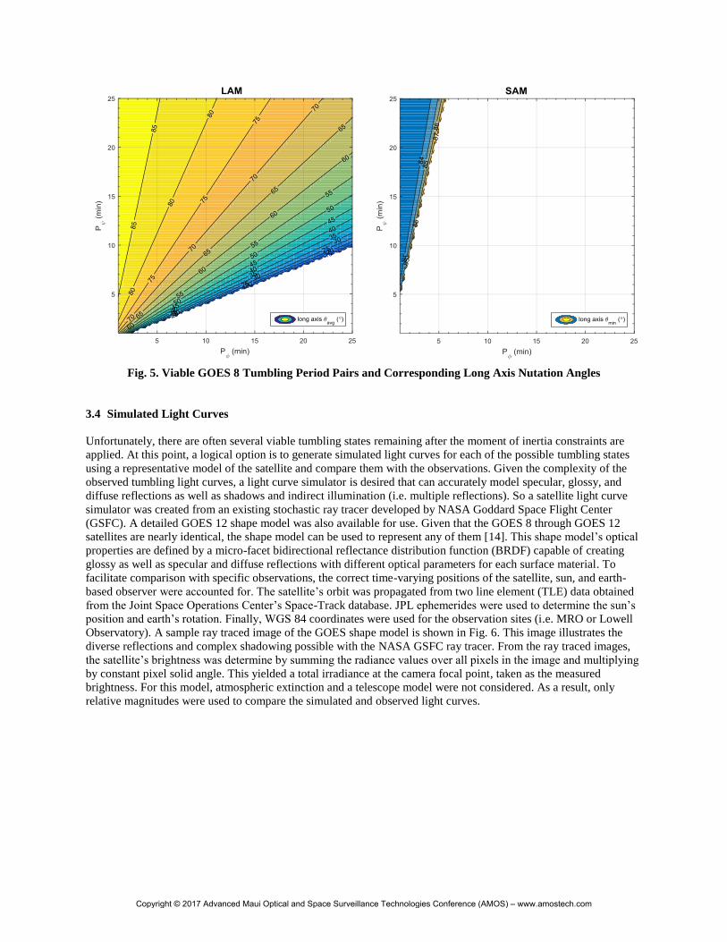
moments of inertia respectively. Using these known moments of inertia, plots of viable 𝑃�̅� and 𝑃𝜓 pairs for GOES 8

rotation states can generated. Two such plots are provided in Fig. 5. Here, 𝑃�̅� and 𝑃𝜓 are given in the conventions

most consistent with the rotation state, long axis for LAMs and short axis for SAMs. Impossible period pairs are

denoted by the white regions. Also included in the plot is the average or minimum long axis nutation angle 𝜃 for

each viable period pair [8]. The closer 𝜃 is to 0°, the closer the satellite is to uniform rotation about its long axis (the

maximum energy state for a given angular momentum 𝐻). The closer 𝜃 is to 90°, the closer to uniform rotation

about the axis of maximum inertia (the minimum energy state for a given 𝐻). Fig. 5 shows that many more period

pairs are viable for LAMs than SAMs. This is due to GOES 8’s nearly prolate moments of inertia, 𝐼𝑠 ≈ 𝐼𝑖 > 𝐼𝑙. These inertia constraints will be leveraged when analyzing the observations.


Fig. 5. Viable GOES 8 Tumbling Period Pairs and Corresponding Long Axis Nutation Angles

3.4 Simulated Light Curves

Unfortunately, there are often several viable tumbling states remaining after the moment of inertia constraints are

applied. At this point, a logical option is to generate simulated light curves for each of the possible tumbling states

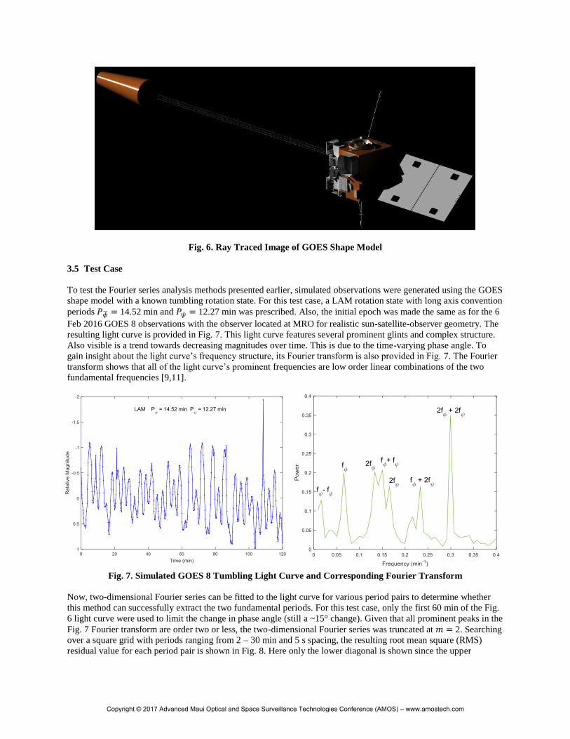
using a representative model of the satellite and compare them with the observations. Given the complexity of the

observed tumbling light curves, a light curve simulator is desired that can accurately model specular, glossy, and

diffuse reflections as well as shadows and indirect illumination (i.e. multiple reflections). So a satellite light curve

simulator was created from an existing stochastic ray tracer developed by NASA Goddard Space Flight Center

(GSFC). A detailed GOES 12 shape model was also available for use. Given that the GOES 8 through GOES 12

satellites are nearly identical, the shape model can be used to represent any of them [14]. This shape model’s optical

properties are defined by a micro-facet bidirectional reflectance distribution function (BRDF) capable of creating

glossy as well as specular and diffuse reflections with different optical parameters for each surface material. To

facilitate comparison with specific observations, the correct time-varying positions of the satellite, sun, and earth-

based observer were accounted for. The satellite’s orbit was propagated from two line element (TLE) data obtained

from the Joint Space Operations Center’s Space-Track database. JPL ephemerides were used to determine the sun’s

position and earth’s rotation. Finally, WGS 84 coordinates were used for the observation sites (i.e. MRO or Lowell

Observatory). A sample ray traced image of the GOES shape model is shown in Fig. 6. This image illustrates the

diverse reflections and complex shadowing possible with the NASA GSFC ray tracer. From the ray traced images,

the satellite’s brightness was determine by summing the radiance values over all pixels in the image and multiplying

by constant pixel solid angle. This yielded a total irradiance at the camera focal point, taken as the measured

brightness. For this model, atmospheric extinction and a telescope model were not considered. As a result, only

relative magnitudes were used to compare the simulated and observed light curves.


Fig. 6. Ray Traced Image of GOES Shape Model

3.5 Test Case

To test the Fourier series analysis methods presented earlier, simulated observations were generated using the GOES

shape model with a known tumbling rotation state. For this test case, a LAM rotation state with long axis convention

periods 𝑃�̅� = 14.52 min and 𝑃𝜓 = 12.27 min was prescribed. Also, the initial epoch was made the same as for the 6

Feb 2016 GOES 8 observations with the observer located at MRO for realistic sun-satellite-observer geometry. The

resulting light curve is provided in Fig. 7. This light curve features several prominent glints and complex structure.

Also visible is a trend towards decreasing magnitudes over time. This is due to the time-varying phase angle. To

gain insight about the light curve’s frequency structure, its Fourier transform is also provided in Fig. 7. The Fourier

transform shows that all of the light curve’s prominent frequencies are low order linear combinations of the two

fundamental frequencies [9,11].

Fig. 7. Simulated GOES 8 Tumbling Light Curve and Corresponding Fourier Transform

Now, two-dimensional Fourier series can be fitted to the light curve for various period pairs to determine whether

this method can successfully extract the two fundamental periods. For this test case, only the first 60 min of the Fig.

6 light curve were used to limit the change in phase angle (still a ~15° change). Given that all prominent peaks in the

Fig. 7 Fourier transform are order two or less, the two-dimensional Fourier series was truncated at 𝑚 = 2. Searching

over a square grid with periods ranging from 2 – 30 min and 5 s spacing, the resulting root mean square (RMS)

residual value for each period pair is shown in Fig. 8. Here only the lower diagonal is shown since the upper


diagonal will just be a reflection of these values over the line 𝑃1 = 𝑃2. The plot shows that a small subset of the

period pairs (those in dark blue) fit the light curve significantly better than the rest.

Fig. 8. RMS Residuals for Fourier Series Fits to Simulated GOES 8 Light Curve (𝒎 = 2) and Best Fit

Finding the local minimum of each dark blue basin with a linearized/iterative least squares algorithm, the best fitting

period pairs were found to be: 1) 𝑃1 = 12.47 min 𝑃2 = 6.69 min, 2) 𝑃1 = 14.41 min 𝑃2 = 6.67 min, and 3) 𝑃1 =14.40 min 𝑃2 = 12.46 min. It is important to note that 1/6.68 ≅ 1/14.40 + 1/12.46. So the frequencies

corresponding to these three well-fitting periods are linearly related. Given this relationship, it is easy to see why all

three pairs fit similarly well, as the terms in their respective Fourier series will have many of the same frequencies.

Determining the correct period pair and which of the four possible tumbling states it represents requires applying the

moment of inertia constraints and generating simulated light curves to see which state best replicates the observed

light curve structure. At this point, it is important to note that 𝑃1 = 14.40 min 𝑃2 = 12.46 min pair fits the light

curve slightly better than the other two pairs and is almost equal to the prescribed pair. The Fourier series fit for

𝑃1 = 14.40 min 𝑃2 = 12.46 min is shown in Fig. 8 and closely matches the observations. The discrepancy between

this pair and the truth is likely due to the time-varying phase angle. Nevertheless, these observed periods differ from

the true periods by less than 2%. This demonstrates that while simple, two dimensional Fourier series fits can

provide reasonable estimates for the fundamental periods, even if the observations span a significant range of phase

angles (~15° for this test case).

4. ANALYSIS

The preceding methods for extracting tumbling rotation states and constraining the possible solutions will now be

applied to the non-periodic GOES 8 light curves. In the following analysis unless otherwise specified, LAM states

will be described in the long axis period convention and SAM states in the short axis convention. This approach is

consistent with conventions for the moment of inertia constraints in Fig. 5.

4.1 12 September 2015

Given that the 12 Sept 2015 observations are in two segments (a,b) with a ~35 min observation gap and significant

change in mean magnitude (likely due to the phase angle change), they will be analyzed separately. Nevertheless,

dynamical changes to the satellite’s fundamental periods should be negligible over the combined observation arc. So

at least one particular period pair should fit both segments well. Segment (a) contains relatively few peaks, resulting

in an overwhelming number of similarly good fits. So segment (b) was analyzed first before returning the former.

The Fourier series grid search with 𝑚 = 2 for segment (b) is shown in Fig. 9. Several pairs yield significantly better

fits to the light curve than the rest. The four best fitting pairs are provided in Table 1. As with the test case above,

these pairs’ frequencies are all linearly related. The pair 𝑃1 = 6.70 min and 𝑃2 = 16.69 min provides a slightly better

fit than the other three. Fits for this pair to both 12 Sept 2015 segments are included in Fig. 10. In these plots, the fit


peaks align well with the general light curve variability. Glints and higher frequency features require a higher

Fourier series order to replicate. Here it should be noted that the number of Fourier series coefficients 𝐶0, 𝐶𝑗𝑘, and

𝑆𝑗𝑘 goes as (2𝑚+1)2. With significantly more degrees of freedom, higher order expansions generally yield better fits

at the expense of many more well-fitting solutions to choose between. As illustrated in the test case above, most

prominent light curve frequencies are low order (𝑚 ≤ 2) linear combinations of 𝑓�̅� and 𝑓𝜓. So second order (𝑚 =

2) fits are usually sufficient to model the major light curve structure.

Fig. 9. 12 Sept 2015 (b) 2-D Fourier Series RMS Residuals (𝒎 = 2)

Table 1. 12 Sept 2015 (b) Best Fit Periods

Pair 𝑷𝟏 (min) 𝑷𝟐 (min) Fit RMS

1 6.66 8.33 0.350

2 6.71 11.23 0.363

3 6.70 16.69 0.336

4 8.36 11.17 0.353

Fig. 10. 12 Sept 2015 (a,b) Best Fit

To help narrow down the 16 candidate rotation states in Table 1 (two LAM and two SAM for each pair), moment of

inertia constraints will be applied. For short axis convention SAM periods, 𝑃𝜓/𝑃�̅� > 2 for all real bodies [9]. This

constraint immediately eliminates seven of the eight candidate SAM states from Table 1. Unfortunately, long axis

convention LAM periods do not have an equally useful general constraint [8]. Leveraging GOES 8’s particular

moments of inertia, the remaining candidate states are analyzed using Fig. 5. First of all, these plots show that the


final candidate SAM state is not possible for GOES 8. Unfortunately, the GOES 8 inertia constraints do not reduce

the possible LAM states in this case. Nevertheless, Fig. 5 shows that 𝜃𝑎𝑣𝑔 for these states will be quite different. For

the two LAM states corresponding to period pair 3, 𝜃𝑎𝑣𝑔 is 14° and 81° respectively. Overall, given that pair 3 fits

the observations best, the most plausible rotation states for the 12 Sept 2015 light curve are LAM with 𝑃�̅� = 6.70

min 𝑃𝜓 = 16.69 min or 𝑃�̅� = 16.69 min 𝑃𝜓 = 6.70 min.

4.2 6 February 2016

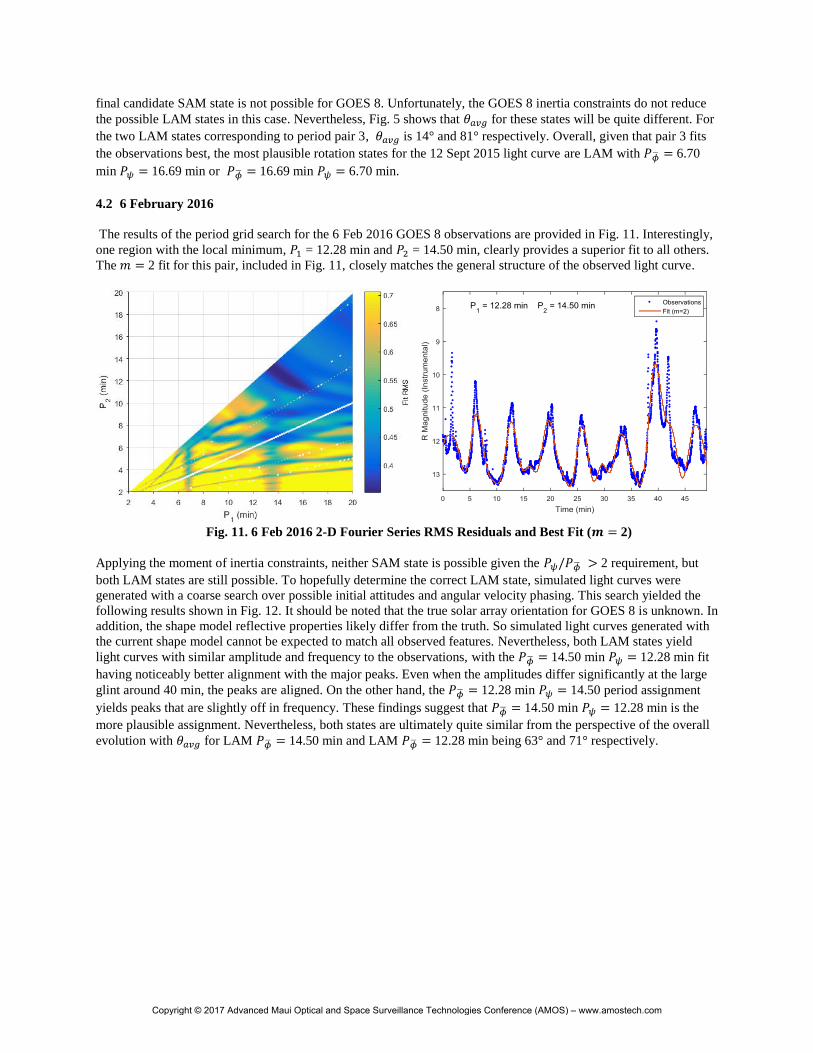
The results of the period grid search for the 6 Feb 2016 GOES 8 observations are provided in Fig. 11. Interestingly,

one region with the local minimum, 𝑃1 = 12.28 min and 𝑃2 = 14.50 min, clearly provides a superior fit to all others.

The 𝑚 = 2 fit for this pair, included in Fig. 11, closely matches the general structure of the observed light curve.

Fig. 11. 6 Feb 2016 2-D Fourier Series RMS Residuals and Best Fit (𝒎 = 2)

Applying the moment of inertia constraints, neither SAM state is possible given the 𝑃𝜓/𝑃�̅� > 2 requirement, but

both LAM states are still possible. To hopefully determine the correct LAM state, simulated light curves were

generated with a coarse search over possible initial attitudes and angular velocity phasing. This search yielded the

following results shown in Fig. 12. It should be noted that the true solar array orientation for GOES 8 is unknown. In

addition, the shape model reflective properties likely differ from the truth. So simulated light curves generated with

the current shape model cannot be expected to match all observed features. Nevertheless, both LAM states yield

light curves with similar amplitude and frequency to the observations, with the 𝑃�̅� = 14.50 min 𝑃𝜓 = 12.28 min fit

having noticeably better alignment with the major peaks. Even when the amplitudes differ significantly at the large

glint around 40 min, the peaks are aligned. On the other hand, the 𝑃�̅� = 12.28 min 𝑃𝜓 = 14.50 period assignment

yields peaks that are slightly off in frequency. These findings suggest that 𝑃�̅� = 14.50 min 𝑃𝜓 = 12.28 min is the

more plausible assignment. Nevertheless, both states are ultimately quite similar from the perspective of the overall

evolution with 𝜃𝑎𝑣𝑔 for LAM 𝑃�̅� = 14.50 min and LAM 𝑃�̅� = 12.28 min being 63° and 71° respectively.


Fig. 12. Observed and Simulated 6 Feb 2016 GOES 8 Light Curves

4.3 3 July 2016

The two-dimensional Fourier series grid search results for the 3 Jul 2016 GOES 8 light curve are plotted in Fig. 13.

There is a small region centered on 𝑃1 = 3.66 min 𝑃2 = 8.61 with significantly better fits. The best fit light curve for

these periods is shown in the right plot of Fig. 13. Although the observations are sparse and a significant gap is

present, the fit closely matches all major variations (the flat segment in the observations at ~2 min is due to

contaminated points that were removed).

Fig. 13. 3 Jul 2016 2-D Fourier Series RMS Residuals and Best Fit (𝒎 =2)

Applying the moment of inertia constraints, neither SAM state is possible for GOES 8’s nearly prolate moments of

inertia. Both LAM states are possible though, with 𝜃𝑎𝑣𝑔 for 𝑃�̅� = 3.66 min and 𝑃�̅� = 8.61 min being 80° and 24°

respectively.

4.4 14 July 2016

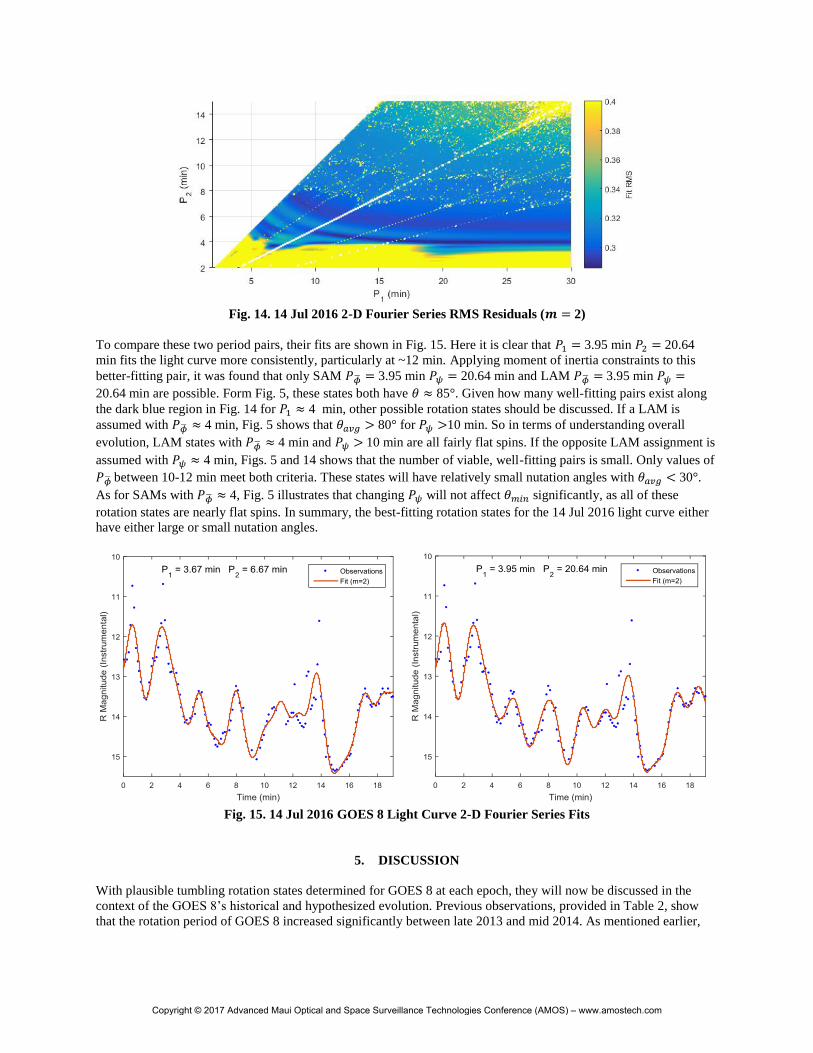
The two-dimensional Fourier series grid search results for the 14 Jul 2016 GOES 8 light curve are plotted in Fig.

14. The first observation is that the majority of well-fitting pairs have one period of ~ 4 min. The large dispersion of

well-fitting periods between 10 - 30 min is likely due to the short time-span of the light curve since longer arcs are

needed to resolve longer periods. Overall, the pair with the lowest RMS residual for 𝑚 = 2 is 𝑃1 = 3.95 min 𝑃2 =

20.64 min. Another of the best-fitting pairs is 𝑃1 = 3.67 min 𝑃2 =6.67 min.


Fig. 14. 14 Jul 2016 2-D Fourier Series RMS Residuals (𝒎 = 2)

To compare these two period pairs, their fits are shown in Fig. 15. Here it is clear that 𝑃1 = 3.95 min 𝑃2 = 20.64

min fits the light curve more consistently, particularly at ~12 min. Applying moment of inertia constraints to this

better-fitting pair, it was found that only SAM 𝑃�̅� = 3.95 min 𝑃𝜓 = 20.64 min and LAM 𝑃�̅� = 3.95 min 𝑃𝜓 =

20.64 min are possible. Form Fig. 5, these states both have 𝜃 ≈ 85°. Given how many well-fitting pairs exist along

the dark blue region in Fig. 14 for 𝑃1 ≈ 4 min, other possible rotation states should be discussed. If a LAM is

assumed with 𝑃�̅� ≈ 4 min, Fig. 5 shows that 𝜃𝑎𝑣𝑔 > 80° for 𝑃𝜓 >10 min. So in terms of understanding overall

evolution, LAM states with 𝑃�̅� ≈ 4 min and 𝑃𝜓 > 10 min are all fairly flat spins. If the opposite LAM assignment is

assumed with 𝑃𝜓 ≈ 4 min, Figs. 5 and 14 shows that the number of viable, well-fitting pairs is small. Only values of

𝑃�̅� between 10-12 min meet both criteria. These states will have relatively small nutation angles with 𝜃𝑎𝑣𝑔 < 30°.

As for SAMs with 𝑃�̅� ≈ 4, Fig. 5 illustrates that changing 𝑃𝜓 will not affect 𝜃𝑚𝑖𝑛 significantly, as all of these

rotation states are nearly flat spins. In summary, the best-fitting rotation states for the 14 Jul 2016 light curve either

have either large or small nutation angles.

Fig. 15. 14 Jul 2016 GOES 8 Light Curve 2-D Fourier Series Fits

5. DISCUSSION

With plausible tumbling rotation states determined for GOES 8 at each epoch, they will now be discussed in the

context of the GOES 8’s historical and hypothesized evolution. Previous observations, provided in Table 2, show

that the rotation period of GOES 8 increased significantly between late 2013 and mid 2014. As mentioned earlier,


YORP simulations by Albuja et al. predicted the rotation period to keep increasing, eventually leading to tumbling

motion.

Table 2. GOES 8 Uniform Rotation Evolution

Date Period

12 Dec 2013 16.83 s [2]

27 Feb 2014 16.48 s [2]

24 Apr 2014 22.95 s [3]

25 July 2014 75.66 s [2]

Summarizing the analysis of the previous section, plausible tumbling states for GOES 8 are provided in Table 3

along with the corresponding long axis nutation angle and long axis spin rate 𝜔𝑙 [8]. The strongest constraint on

GOES 8’s tumbling evolution was provided by the 6 Feb 2016 light curve, with LAM 𝑃�̅� = 14.50 min 𝑃𝜓 = 12.28

min yielding a clearly superior Fourier series fit as well as a simulated light curve consistent with the observations.

To transition this far into the LAM regime from uniform rotation, the satellite would require significant spin up

about its long axis. The LAM 𝑃�̅� = 6.70 min state at the 12 Sept 2015 epoch is consistent with this spin up, with

𝜃𝑎𝑣𝑔 decreasing and 𝜔𝑙 increasing. Considering now the two plausible 3 July 2016 solutions, both cases have

significantly lower periods than for 6 Feb 2016 with higher 𝜔𝑙. Again, a transition to either 3 Jul 2016 state would

require additional long axis acceleration. Proceeding to 14 Jul 2016, the plausible LAM and SAM states both have

higher nutation angles than for the 3 Jul 2016 states, indicative of more relaxed motion closer to uniform rotation.

Table 3. Plausible GOES 8 Tumbling Rotation States

Mode 𝑷�̅� (min) 𝑷𝝍 (min) Long Axis 𝜽𝒂𝒗𝒈 𝝎𝒍 (rad/s)

12 Sept 2015

LAM 6.70 16.69 81° 0.00991

LAM 16.69 6.70 14° 0.0217

6 Feb 2016

LAM 14.50 12.28 63° 0.0120

3 Jul 2016

LAM 3.66 8.61 80° 0.019

LAM 8.61 3.66 24° 0.0398

14 Jul 2016

SAM 3.95 20.64 > 85° 0.00703

LAM 3.95 20.64 85° 0.0115

In all, while there are a number of possible evolutionary paths, the best-fitting rotation states do show a general

trend. They suggest that GOES 8 transitioned from uniform motion to an excited long axis mode rotation state

between 25 Jul 2014 and 6 Feb 2016 before returning to a more relaxed state closer to uniform rotation by 14 Jul

2016. This general trend would require the satellite’s long axis spin rate to first increase then decrease, consistent

with the Albuja et al. hypothesis that a tumbling GOES 8 will spin up preferentially about its long axis before energy

dissipation drives it back towards the minimum energy state.

6. CONCLUSION

In an effort to better understand how the YORP effect may drive rotation state evolution of retired geosynchronous

satellites, several non-periodic light curves of the retired GOES 8 satellite were analyzed. Leveraging torque-free

rigid body dynamics, Fourier series frequency analysis, as well as known information about the satellite’s shape and

end of life moments of inertia, plausible tumbling rotation states were found at each observation epoch. Linking

these plausible states together with previous observations suggests that GOES 8 evolved from uniform rotation into

an excited tumbling state before transitioning back towards more relaxed motion. This apparent evolution agrees

with the hypothesis that some retired geosynchronous satellites cycle between uniform and tumbling motion due to

the combined influences of YORP and energy dissipation.


Given the complexity of these non-periodic light curves, more analysis is needed to further validate the plausible

tumbling states at each observation epoch. This will require additional development of the light curve simulator to

efficiently test many simulated light curves simultaneously. Hopefully by searching over smaller increments of

initial attitude, angular velocity phasing, and solar panel orientation, close matches to the GOES 8 observations can

be found. In all, this analysis only offers a glimpse into the evolution of one satellite. To truly understand and predict

the rotation state evolution of GOES 8 and other retired geosynchronous satellites, more observations and dynamical

modeling is needed.

7. ACKNOWLEDGEMENTS

The primary author would like to thank Steven Queen of NASA Goddard Space Flight Center for his assistance in

developing the light curve simulator. In addition, this work was supported by a NASA Space Technology Research

Fellowship.

8. REFERENCES

1. Papushev, P., Karavaev, Y., Mishina, M., Investigations of the evolution of optical characteristics and

dynamics of proper rotation of uncontrolled geostationary artificial satellites, Advances in Space Research, Vol.

43(9), 1416–1422, 2009.

2. Cognion, R., Rotation rates of inactive satellites near geosynchronous earth orbit, Proceedings of the 2014

Advanced Maui Optical and Space Surveillance Technologies Conference, 2014.

3. Ryan, W.H., Ryan, E.V., Photometric Studies of Rapidly Spinning Decommissioned GEO Satellites,

Proceedings of the 2015 Advanced Maui Optical and Space Surveillance Technologies Conference, 2015.

4. Albuja, A.A., Scheeres, D.J., McMahon, J.W., Evolution of angular velocity for defunct satellites as a result of

YORP: An initial study, Advances in Space Research, Vol. 56(2), 237–251, 2015.

5. Albuja, A., Rotational Dynamics of Inactive Satellites as a Result of the YORP Effect, Aerospace Engineering

Sciences Graduate Theses & Dissertations (2015), 113, http://scholar.colorado.edu/asen_gradetds/113,

retrieved Sept. 9, 2017.

6. Albuja, A.A., Scheeres, D.J., Cognion, R., Ryan, W.H., Ryan, E.V., The YORP Effect on the GOES 8 and

GOES 10 Satellites: A Case Study, Advances in Space Research, (in review)

7. Benson, C.J., Scheeres, D.J., Moskovitz, N., Light curves of retired geosynchronous satellites, Proceedings of

the 7th European Conference on Space Debris, 2017.

8. Samarasinha, N.L., A’Hearn, M.F., Observational and Dynamical Constraints on the Rotation of Comet

P/Halley, Icarus, Vol. 93(2), 194-225, 1991.

9. Samarasinha, N.L., Mueller, B.E.A., Component periods of non-principal-axis rotation and their manifestations

in the lightcurves of asteriods and bare cometary nuclei, Icarus, Vol. 248, 347-356, 2015.

10. Benson, C.J., Scheeres, D.J., Extraction and assignment of tumbling asteroid and defunct satellite rotation

periods from simulated light-curve observations, Proceedings of the 27th AAS/AIAA Space Flight Mechanics

Meeting, 2017.

11. Kaasalainen, M., Intepretation of lightcurves of precessing asteroids, Astronomy and Astrophysics, Vol. 376(1),

302-309, 2001.

12. Pravec, P. et al., Tumbling Asteroids, Icarus, Vol. 173(1), 108-131, 2005.

13. Landau, L.D., and Lifshitz, E.M., Mechanics, Vol. 1. Oxford, England: Pergamon Press, 2nd ed., 1969.

14. GOES I-M Databook, Rev. 1, Aug. 31, 1996, https://goes.gsfc.nasa.gov/text/goes.databook.html, retrieved

Sept. 9, 2017.


Date post:	17-Jan-2020
Category:	Documents
Upload:	others
View:	11 times
Download:	0 times

Rotation state evolution of retired geosynchronous ... · drives rotation state evolution of...

Documents