ROTI Maps: a new IGS’s ionospheric product characterizing the ionospheric irregularities occurrence Iurii Cherniak Andrzej Krankowski Irina Zakharenkova Space Radio-Diagnostic Research Center, University of Warmia and Mazury, Olsztyn, Poland 3 - 7 July 2017
Transcript
ROTI Maps: a new IGS’s ionospheric product characterizing the ionospheric irregularities
Space Radio-Diagnostic Research Center, University of Warmia and Mazury, Olsztyn, Poland
3 - 7 July 2017
Image credit: UWM
Ionosphere is the part of the Earth’s atmosphere, consisting of several ionized layers and extending from about 50 km up to 1,000 km.Plasma density distribution in the ionosphere varies with:
• altitude• day/night• seasons• latitude/longitude• solar activity• geomagnetic conditions
Ionosphere-plasmasphere system (courtesy of the Windows to the Universe)
Electron density distribution with altitude
Global ionospheric maps of total electroncontent (TEC) – IGS GIMs
Equatorial Region: strongest effects; highest; strongest TEC gradients; Irregularities not correlated with magnetic activity
Mid-Latitude Region: normally quiescent but with strong gradients during extreme levels of geomagnetic activity
Auroral Region: aurora and structures. Phase scintillations.
Introduction. Ionosphere
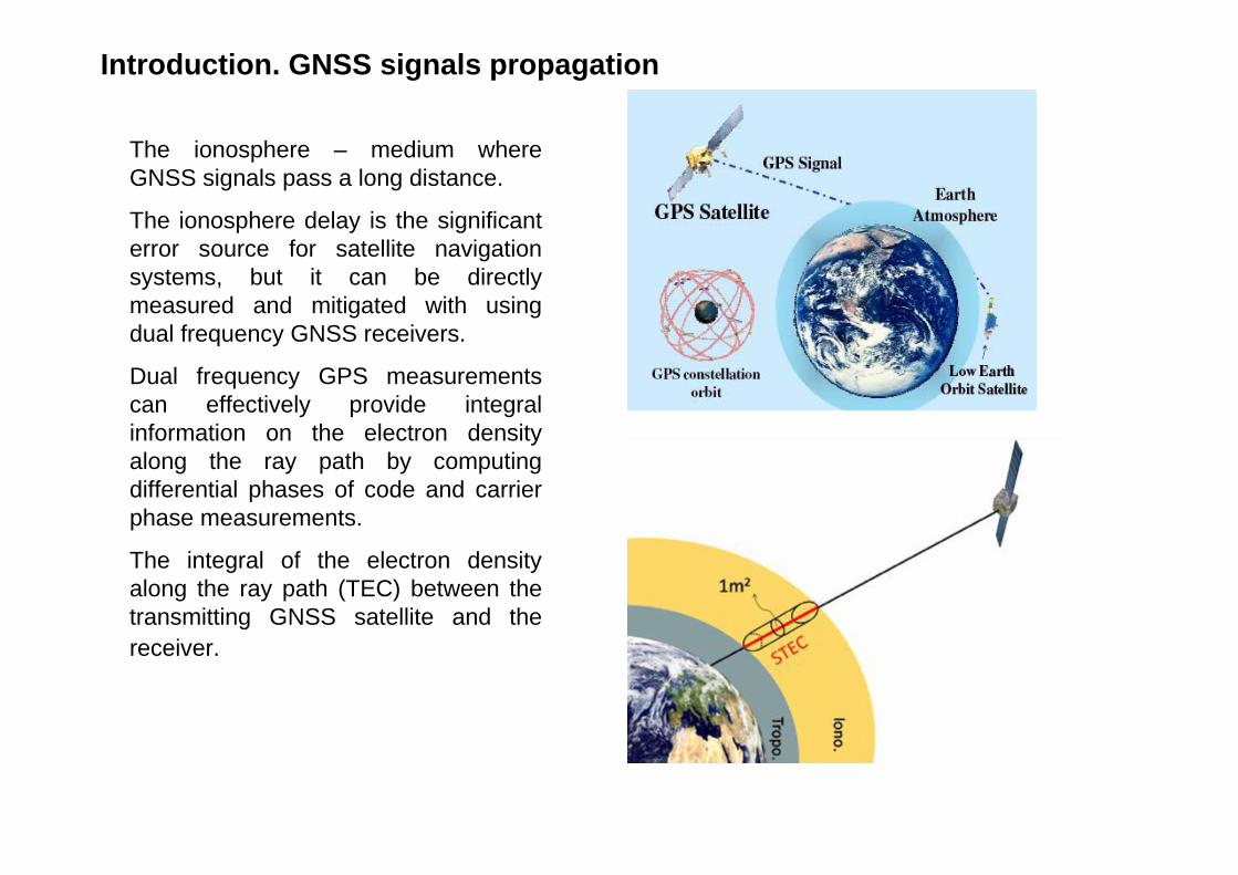
The ionosphere – medium where GNSS signals pass a long distance.
The ionosphere delay is the significant error source for satellite navigation systems, but it can be directly measured and mitigated with using dual frequency GNSS receivers.
Dual frequency GPS measurements can effectively provide integral information on the electron density along the ray path by computing differential phases of code and carrier phase measurements.
The integral of the electron density along the ray path (TEC) between the transmitting GNSS satellite and the receiver.
Introduction. GNSS signals propagation
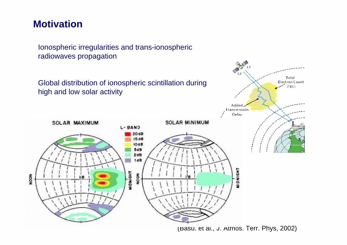
(Basu. et al., J. Atmos. Terr. Phys, 2002)
Motivation
Ionospheric irregularities and trans-ionospheric radiowaves propagation
Global distribution of ionospheric scintillation during high and low solar activity
The open questions:
When and where high-latitude ionospheric plasma irregularities are developed?
Our task:
Monitoring of the ionospheric irregularities over the Northern Hemisphere.
Our approach:
The TEC rapid changes analysis on the base of GPS signal measurements
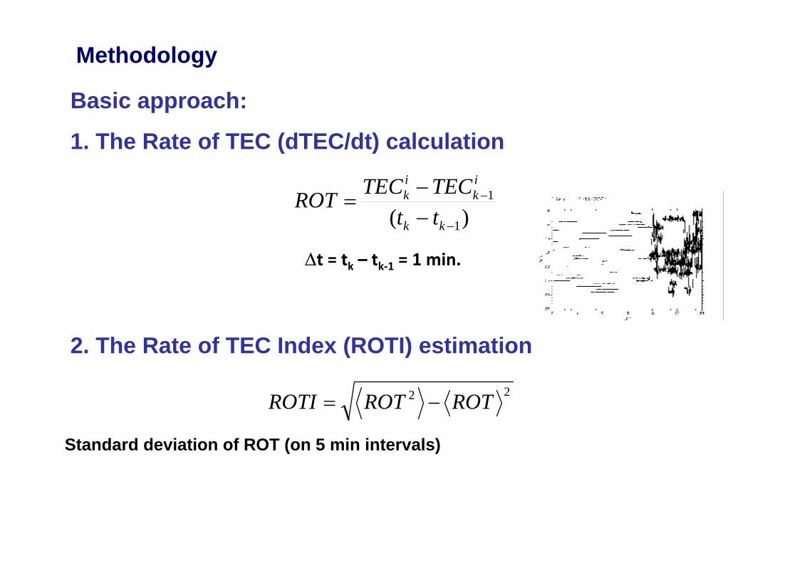
Basic approach:
1. The Rate of TEC (dTEC/dt) calculation
2. The Rate of TEC Index (ROTI) estimation
∆t = tk – tk‐1 = 1 min.
22 ROTROTROTI −=
Standard deviation of ROT (on 5 min intervals)
)( 1
1
−
−
−−
=kk
ik
ik
ttTECTECROT
Methodology
Methodology
Data sources:
UNAVCO
IGS
> 700 stations
Methodology
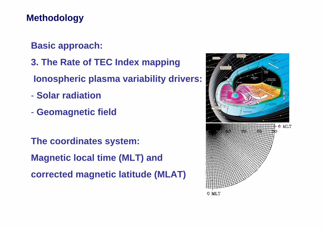
Basic approach:
3. The Rate of TEC Index mapping
Ionospheric plasma variability drivers:
- Solar radiation
- Geomagnetic field
The coordinates system:
Magnetic local time (MLT) and
corrected magnetic latitude (MLAT)
Methodology
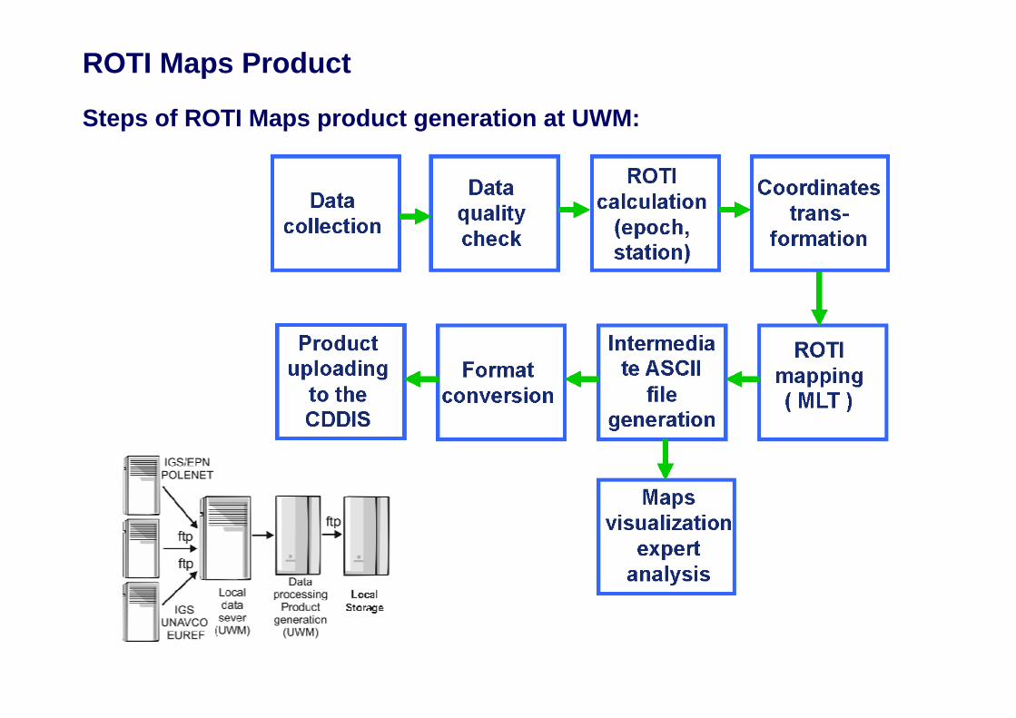
Steps of ROTI Maps product generation at UWM:
ROTI Maps Product
5h 40 minTotal
5 minFinal productgeneration4
2,5hData processing3
1hQuality check2
2hData collection1
Processingtime
Processing phaseN
Avaliable24h
Non avaliable12hGPS orbit data
ftp://cddis.gsfc.nasa.gov/pub/gps/products/
75%20h
50%12h
30%6hGPS observations
ftp://data-out.unavco.org/pub/rinex/obs/
ftp://epncb.oma.be/pub/obs/
AvailabilityLatencyInput data
The product latency is determined on the input data availabilityand it takes more 48 h.
The ROTI Maps latency
Steps of ROTI Maps product generation at UWM:
ROTI Maps Product
The sample of the ROTI Maps output: ASCII format.
The output maps provided in the ASCII formats. This data prepared in the IONEX-like format on grid 2 x 2 degree - geomagnetic latitude from 51o to 89o with step 2o and corresponded to magnetic local time (00-24 MLT) polar coordinates from 0 to 359.
ROTI Maps format
ROTI Maps Product
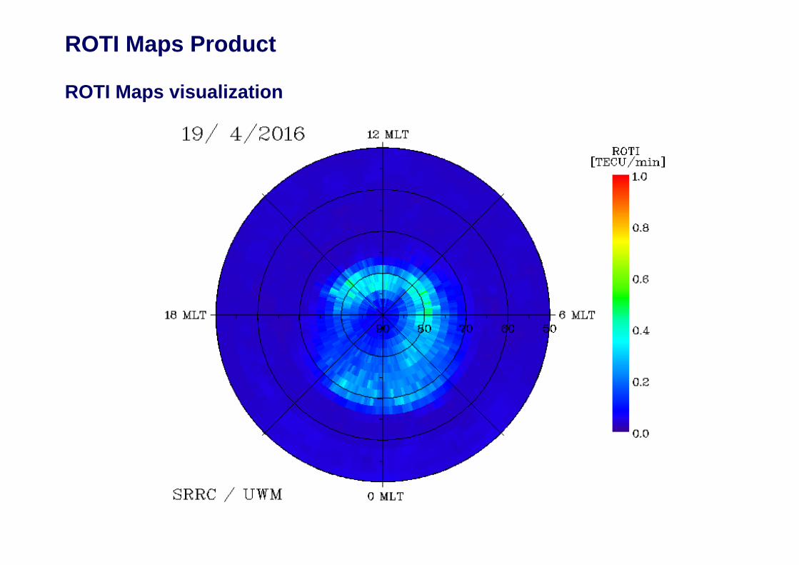
ROTI Maps visualization
ROTI Maps Product
ROTI Maps visualization
ROTI Maps Product
ROTI Maps visualization
ROTI Maps Product
It was processed and collected data and resulted product from 2010up to now since the test service established.
There is no gaps in the ROTI Maps product dataset for test period.
The ROTI maps product validation activity on 2015-2016 dataset.
ROTI Maps product for 2016 – 2017 available since March 2017 on CDDIS.
Detailed description of the ROTI Maps Product will be available in paper Cherniak et al., GPS Solution, 2017 (under review).
The UWM ROTI Maps processor operates routinely since January, 1, 2015.
The ROTI Maps product generation at UWM:
ROTI Maps Product
Cherniak et al., GPS Solution, 2017
ROTI Maps Product
The ROTI maps product have been validated within framework of Monitor-2 European Space Agency Project(2015-2016 dataset).Beniguel et al., 2016, AnnGeo.
2015 St. Patrick’s Day Storm
Largest storm for last 10 years
Intense particle precipitation
Aurora was registered at mid-latitudes
(Cherniak et al,, AGU SW, 2015
ROTI Maps Product. Scientific Applications.
B. Wanner, WAAS Technical Report:“Iono activity affected WAAS performance inCanada, Alaska, and CONUS on March 17 andMarch 18”
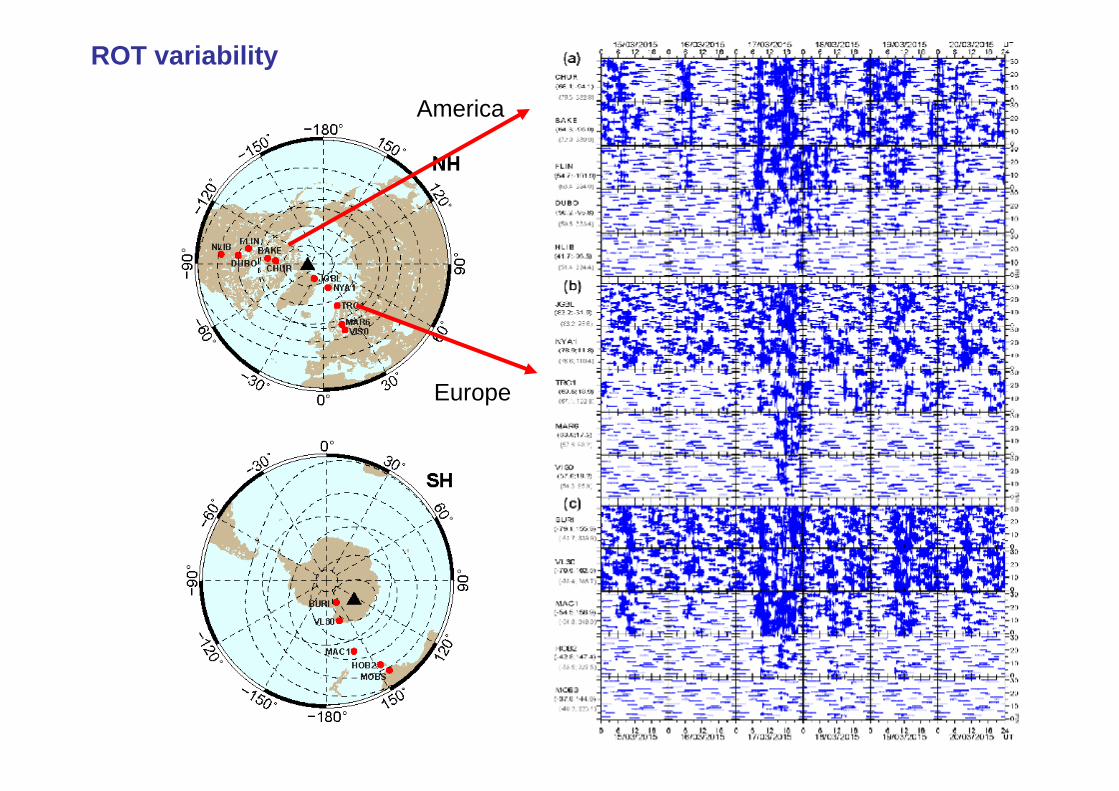
ROT variability
America
Europe
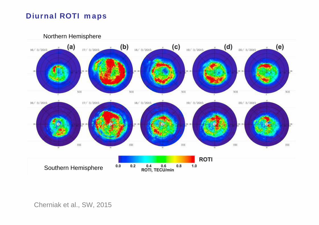
Northern Hemisphere
Diurnal ROTI maps
Cherniak et al., SW, 2015
Southern Hemisphere
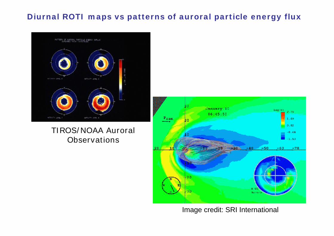
Diurnal ROTI maps vs patterns of auroral particle energy flux
TIROS/NOAA Auroral Observations
Image credit: SRI International
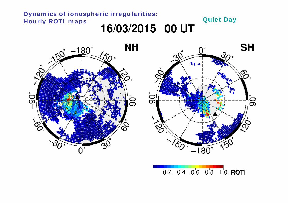
Dynamics of ionospheric irregularities: Hourly ROTI maps Quiet Day
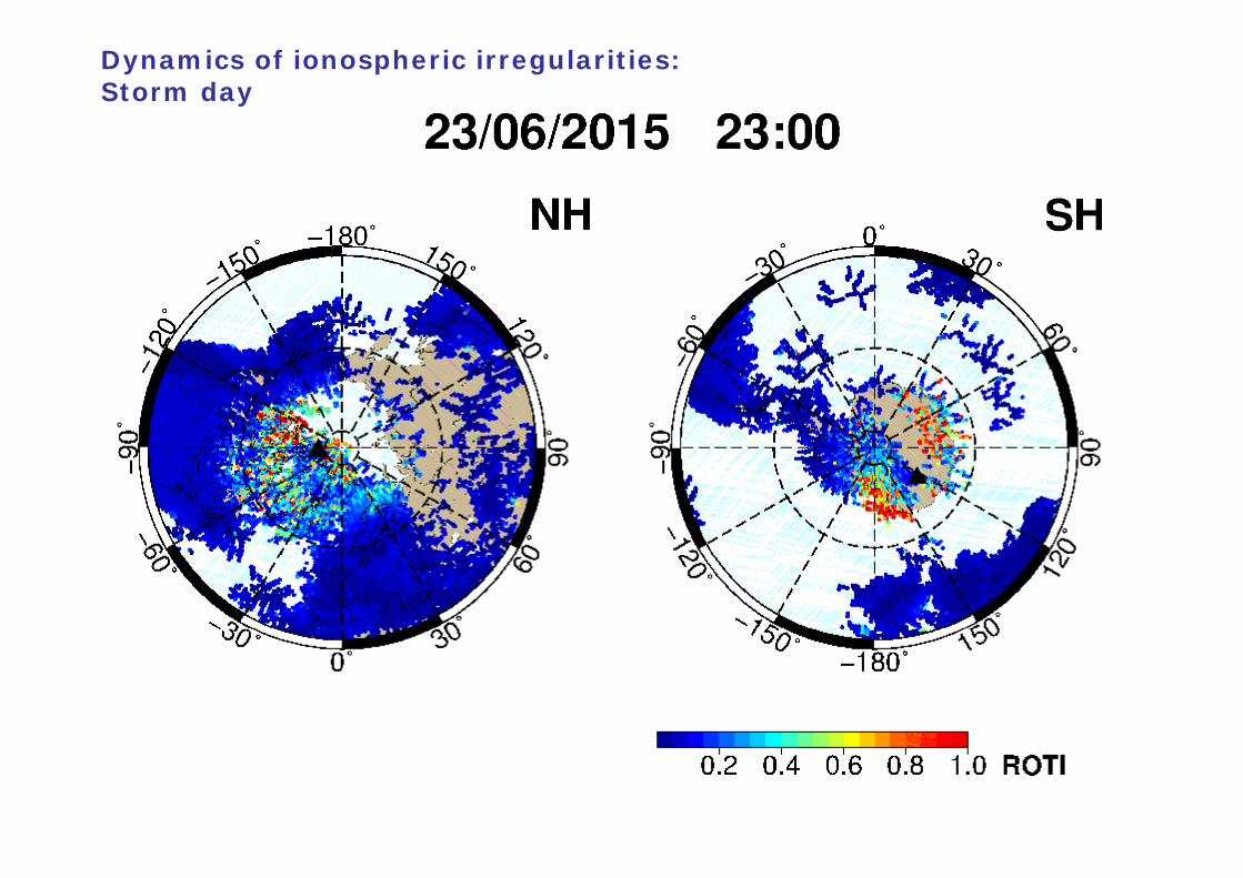
Dynamics of ionospheric irregularities: Storm day
SED/TOI
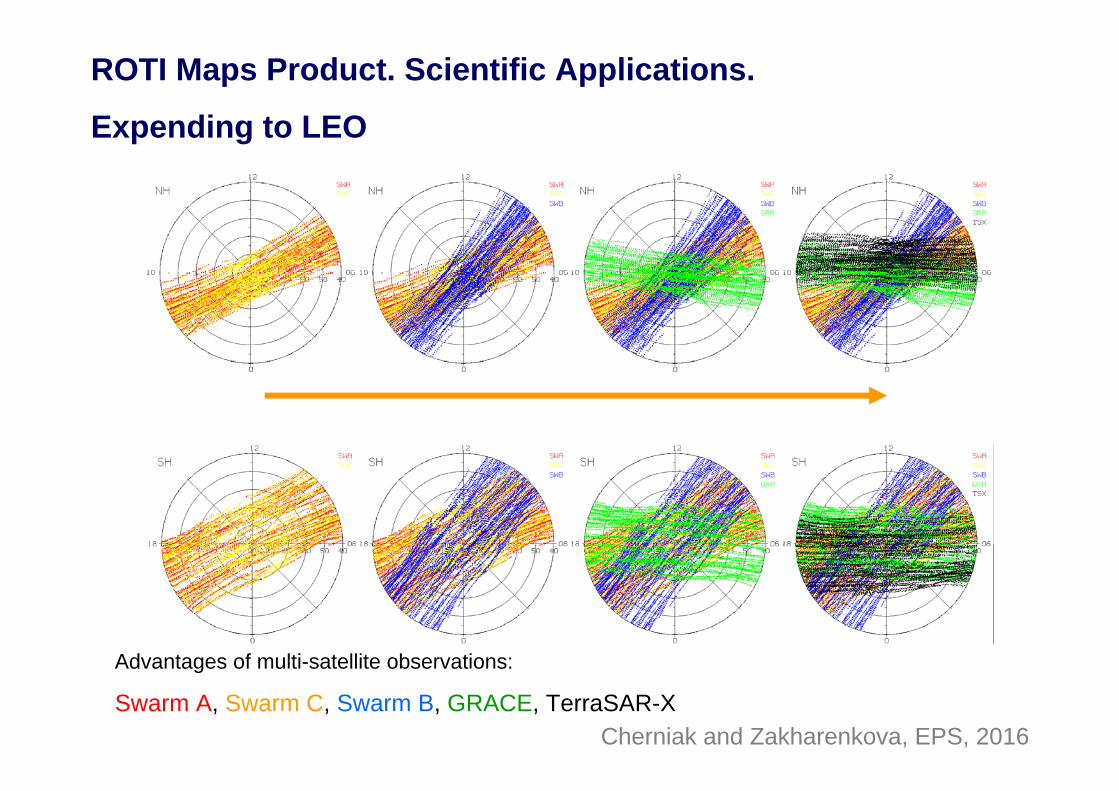
Advantages of multi-satellite observations:
Swarm A, Swarm C, Swarm B, GRACE, TerraSAR-XCherniak and Zakharenkova, EPS, 2016
ROTI Maps Product. Scientific Applications.
Expending to LEO
Duirnal ROTI maps: Ground GPS vs LEO GPS
Application of ROTI mapping technique to LEO GPS measurements.
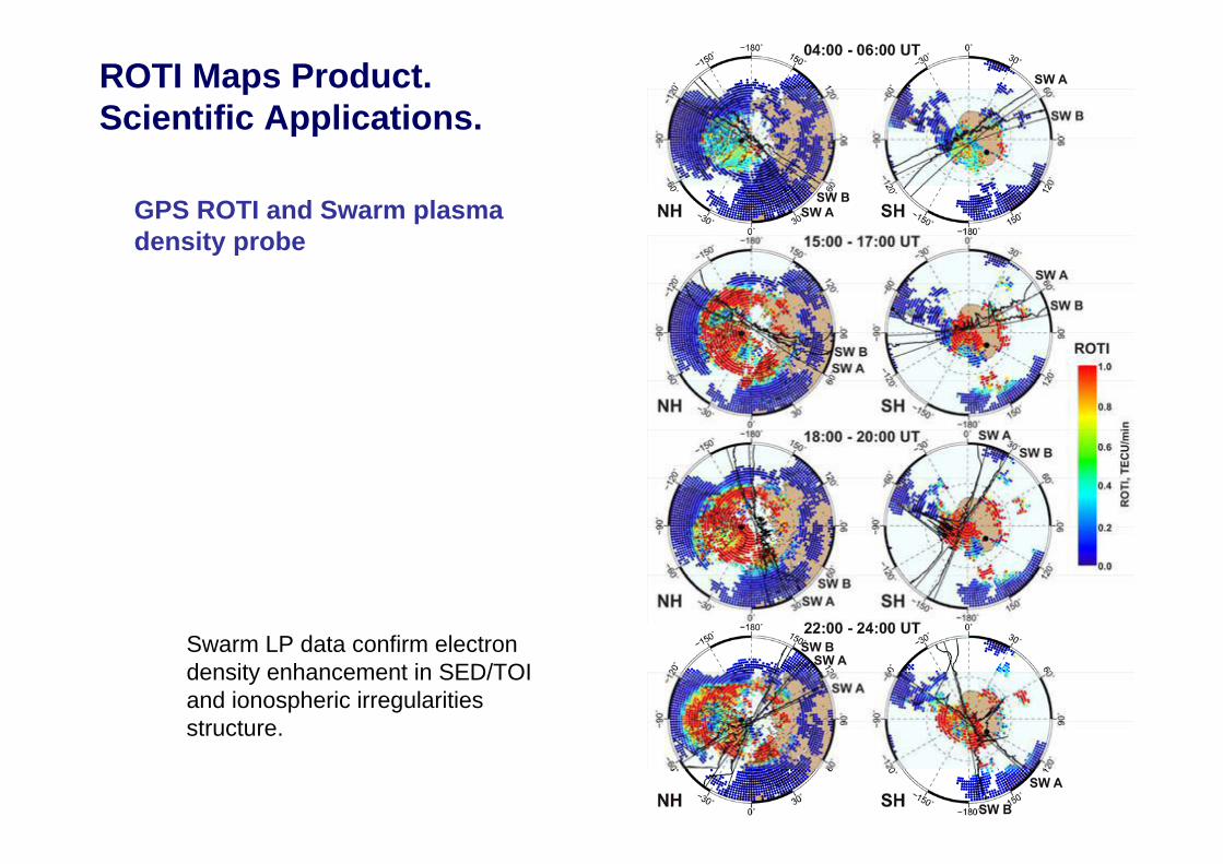
Swarm LP data confirm electron density enhancement in SED/TOI and ionospheric irregularities structure.
GPS ROTI and Swarm plasma density probe
ROTI Maps Product. Scientific Applications.
SuperDARN polar potential maps for the Southern Hemisphere at a 18.4 UT and b 18.8 UT, and the Northern Hemisphere at c 18.0 UT with superimposed low earth orbit (LEO) Rate of TEC (ionospheric total electron content) index (ROTI) (colored lines) and in situ (thick black line) observations.
Black dot indicates the position of the magnetic pole.
The right-hand panel shows Swarm electron density (Ne) and LEO TEC variations for corresponding tracks on the maps. UT and geographic latitude and longitude are noted at the bottom axes.
Data tracks are line of sight between twopoints, e.g., “SWA-GPS 19” denotes the data between SWA and GPS PRN 19. TEC data are the relative slant TEC measurements. ROTI is shown in unitsof TECU/min. Minutes are indicated in decimal format
-250
-150
-50
50
SY
M-H
(nT)
-40-30-20-10
010203040
Bz
(nT)
0500
1000150020002500
AE
(nT)
20 21 22 23 24
300400500600700800
Vsw
(km
/s)
0
20
40
60
Psw
(nP
a)
June 2015
June 2015 Storm
Diurnal ROTI maps
Dynamics of ionospheric irregularities: Quiet day
Dynamics of ionospheric irregularities: Storm day
Two-dimensional ROTI maps of ionospheric irregularities in geographic coordinates over Europe with 1 h interval during 18 UT–05 UT on 22–23 June 2015.
(b) Two-dimensional maps of vertical TEC with superimposed Swarm A and Swarm B passes (magenta lines) for 23 UT and 01 UT, respectively; in situ electron density and topside vertical TEC along these passes are shown at small panels on the right. Numerous plasma depletions are embedded into high TEC plasma within 25°–40°N.
Cherniak and Zakharenkova, GRL, 2016
The (left) global view with Swarm A satellite passes and spaceborne GPS ROTI;
(right) variation of in situ electron density Neas a function of geographical latitude along these passes.
Black lineson latitudinal profiles present Ne values for 22–23 June; thin blue lines are quiet-time conditions of 20–21 June 2015.
Universal time (UT) and geographic longitude for each satellite pass are given at the top of graphs.
The yellow shaded areaindicates deep plasma depletions in Europe and its close vicinity. (b) The same as Figure 1a but for Swarm B satellite. (c)
The passes of DMSP F15, F17, and F18 satellites (left) and in situ ion density variations along these passes (right). On eachgeographic map, grid with 30° is shown by thin dashed line; geomagnetic equator is shown by black solid line.
Conclusions- The indices and maps, based on GPS ROT/ROTI variations, can be effective and very perspective indicator of the presence of phase fluctuations in the high and mid-latitude ionosphere.
- ROTI maps allow to estimate the overall fluctuation activity and auroral oval evolutions, the values of ROTI index corresponded to probability of GPS signals phase fluctuations
- The applied approach for ROTI map construction does not use any interpolation technique for ROTI mapping, result is real observations, averaged in each cell of 2 x 2 deg. This will allow to avoid errors related with unrealistic interpolation values over areas with data gaps.
- The results demonstrate that it is possible to use current network of GNSS permanent stations to reveal the ionospheric irregularities intensity, and position of the irregularities oval.
- The ROTI maps product have been validated against different types of ground and sattelitebased measurements.
-The ROTI Maps product available since March 2017 on CDDIS.
- Detailed description of the ROTI Maps Product will be available in paper “ROTI Maps: a new IGS’s ionospheric product characterizing the ionospheric irregularities occurrence” by Iu. Cherniak, A. Krankowski, I. Zakharenkova:, GPS Solution, 2017 (under review).
We acknowledge use of the raw GPS data provided by IGS (ftp://cddis.gsfc.nasa.gov), UNAVCO (ftp://data-out.unavco.org), EUREF (ftp://rgpdata.ign.fr).
The authors are grateful for the CODE for the Rapid IGS product with GPS orbit data.
The authors thank the NASA/GSFC's Space Physics Data Facility's OMNIWeb service, for providing OMNI data (ftp://spdf.gsfc.nasa.gov/pub/data/omni) and program code for CGM coordinates calculation.
The AE and Kp indices are provided by the World Data Center for Geomagnetism, Kyoto University (wdc.kugi.kyoto-u.ac.jp).