1 INTRODUCTION 1.1Analysis of piles using Winkler method In Winkler method (Beam on Non- linear Winkler Foundation) of analysis of piles, the pile-soil interactions are represented by a set of nonlinear soil springs: p-y springs (commonly known as curves incorporates the lateral pile-soil interaction), t-z springs (models the shaft resistance i.e. pile-soil friction) and q-z spring (models the end-bearing interaction). Figure 1 shows a simple model of a pile which can be analyzed using any standard structural software and can incorporate advanced features such as P-delta effects, non-linearity in the material of the pile. For any load or displacement applied to the pile either at the pile head (represents inertia load from the superstructure) or along the pile, the required analysis outputs are pile deflection, rotation, bending moment, shear and soil reaction. However, undoubtedly the critical inputs for a realistic analysis are the springs which represents the interactions. This paper deals with p-y springs/curves for seismically liquefied soil and explores method for its construction. p-y springs are generally constructed using a set of scaling rules as prescribed by codes of practice and necessary input parameters are obtained from stress-strain of the soil. The next section reviews the methods for constructing p-y curves for sand, clay and liquefied soils. Winkler springs (p-y curves) for liquefied soil from element tests M. Rouholamin & S. Bhattacharya Department of Civil and Environmental Engineering, University of Surrey, United Kingdom D.Lombardi Department of Civil and Environmental Engineering, Edinburgh Napier University, United Kingdom ABSTRACT: In practice, piles are most often modelled as "Beams on Non- Linear Winkler Foundation" (also known as “p-y spring” approach) where the soil is idealised as p-y springs. These p-y springs are obtained through semi-empirical approach using element test results of the soil. For liquefied soil, a reduction factor (often termed as p-multiplier approach) is applied on a standard p-y curve for the non-liquefied condition to obtain the p-y curve liquefied soil condition. This paper presents a methodology to obtain p-y curves for liquefied soil based on element testing of liquefied soil considering physically plausible mechanisms. Validation of the proposed p-y curves is carried out through the back analysis of physical model tests.
Transcript
1 INTRODUCTION
1.1 Analysis of piles using Winkler method
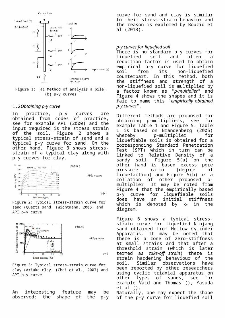
In Winkler method (Beam on Non-linear Winkler Foundation) of analysis of piles, the pile-soil interac-tions are represented by a set of nonlinear soil springs: p-y springs (commonly known as curves in-corporates the lateral pile-soil interaction), t-z springs (models the shaft resistance i.e. pile-soil fric-tion) and q-z spring (models the end-bearing interac-tion). Figure 1 shows a simple model of a pile which can be analyzed using any standard structural soft-ware and can incorporate advanced features such as P-delta effects, non-linearity in the material of the pile. For any load or displacement applied to the pile either at the pile head (represents inertia load from the superstructure) or along the pile, the required analysis outputs are pile deflection, rotation, bending moment, shear and soil reaction. However, un-doubtedly the critical inputs for a realistic analysis are the springs which represents the interactions. This paper deals with p-y springs/curves for seismi-cally liquefied soil and explores method for its con-struction.
p-y springs are generally constructed using a set of scaling rules as prescribed by codes of practice and necessary input parameters are obtained from stress-strain of the soil. The next section reviews the methods for constructing p-y curves for sand, clay and liquefied soils.
Figure 1: (a) Method of analysis a pile, (b) p-y curves
1.2 Obtaining p-y curve
In practice, p-y curves are obtained from codes of practice, see for example API (2000) and the input required is the stress strain of the soil. Figure 2 shows a typical stress-strain of sand and a typical p-y curve for sand. On the other hand, Figure 3 shows stress-strain of a typical clay along with p-y curves for clay.
p(kN/m)
y(m)
API p y curve‐
Winkler springs (p-y curves) for liquefied soil from element tests
M. Rouholamin & S. Bhattacharya
Department of Civil and Environmental Engineering, University of Surrey, United Kingdom
D.Lombardi
Department of Civil and Environmental Engineering, Edinburgh Napier University, United Kingdom
ABSTRACT: In practice, piles are most often modelled as "Beams on Non-Linear Winkler Foundation" (also known as “p-y spring” approach) where the soil is idealised as p-y springs. These p-y springs are ob-tained through semi-empirical approach using element test results of the soil. For liquefied soil, a reduction factor (often termed as p-multiplier approach) is applied on a standard p-y curve for the non-liquefied condi-tion to obtain the p-y curve liquefied soil condition. This paper presents a methodology to obtain p-y curves for liquefied soil based on element testing of liquefied soil considering physically plausible mechanisms. Val -idation of the proposed p-y curves is carried out through the back analysis of physical model tests.
Figure 2: Typical stress-strain curve for sand (Quartz sand, (Wichtmann, 2005) and API p-y curve
Figure 3: Typical stress-strain curve for clay (Ariake clay, (Chai et al., 2007) and API p-y curve
An interesting feature may be observed: the shape of the p-y curve for sand and clay is similar to their stress-strain behavior and the reason is explored by Bouzid et al (2013).
p-y curves for liquefied soilThere is no standard p-y curves for liquefied soil and often a reduction factor is used to obtain empirical p-y curve for liquefied soil from its non-liquefied counterpart. In this method, both the stiffness and strength of a non-liquefied soil is multiplied by a factor known as "p-multiplier" and Figure 4 shows the shapes and it is fair to name this "empirically ob-tained p-y curves".
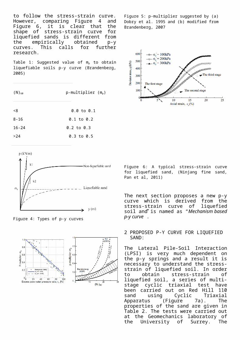
Different methods are proposed for obtaining p-mul-tipliers, see for example Table 1 and Figure 5. Table 1 is based on Brandenberg (2005) whereby p-multi-plier for liquefiable soils is obtained for a corres-ponding Standard Penetration Test (SPT) which in turn can be linked to Relative Density of a sandy soil. Figure 5(a) on the other hand is based excess pore pressure ratio (degree of liquefaction) and Fig-ure 5(b) is a collation of other proposed p-multiplier. It may be noted from Figure 4 that the empirically based p-y curve for liquefiable soils does have an initial stiffness which is denoted by k2 in the dia-gram.
Figure 6 shows a typical stress-strain curve for li-quefied Ninjang sand obtained from Hollow Cylin-der Apparatus. It may be noted that there is a zone of zero-stiffness at small strains and that after a threshold strain (which is later termed as take-off strain) there is strain hardening behaviour of the soil. Similar observations have been reported by other researchers using cyclic triaxial apparatus on other types of sands, see for example Vaid and Thomas (), Yasuda et al ().
Naturally, one may expect the shape of the p-y curve for liquefied soil to follow the stress-strain curve. However, comparing Figure 4 and Figure 6, it is clear that the shape of stress-strain curve for lique-fied sands is different from the empirically obtained p-y curves. This calls for further research.
Table 1: Suggested value of mp to obtain liquefiable soils p-y curve (Brandenberg, 2005)
(N)60 p-multiplier (mp)
<8 0.0 to 0.1
8-16 0.1 to 0.2
16-24 0.2 to 0.3
>24 0.3 to 0.5
Figure 4: Types of p-y curves
Figure 5: p-multiplier suggested by (a) Dobry et al. 1995 and (b) modified from Brandenberg, 2007
p(kN/m)
y(m)
API p-y curve
Figure 6: A typical stress-strain curve for liquefied sand, (Nin-jang fine sand, Pan et al, 2011)
The next section proposes a new p-y curve which is derived from the stress-strain curve of liquefied soil and is named as “Mechanism based p-y curve”.
2 PROPOSED P-Y CURVE FOR LIQUEFIED SAND:
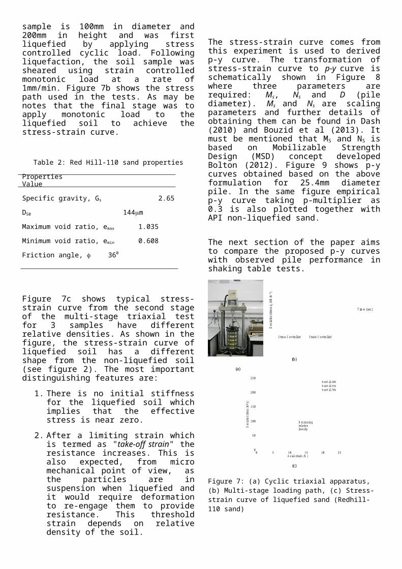
The Lateral Pile-Soil Interaction (LPSI) is very much dependent on the p-y springs and a result it is necessary to understand the stress-strain of liquefied soil. In order to obtain stress-strain of liquefied soil, a series of multi-stage cyclic triaxial test have been carried out on Red Hill 110 sand using Cyclic Triax-ial Apparatus (Figure 7a). The properties of the sand are given in Table 2. The tests were carried out at the Geomechanics laboratory of the University of Surrey. The sample is 100mm in diameter and 200mm in height and was first liquefied by applying stress controlled cyclic load. Following liquefaction, the soil sample was sheared using strain controlled monotonic load at a rate of 1mm/min. Figure 7b shows the stress path used in the tests. As may be notes that the final stage was to apply monotonic load to the liquefied soil to achieve the stress-strain curve.
Table 2: Red Hill-110 sand properties
Properties Value
Specific gravity, Gs 2.65
D50 144m
Maximum void ratio, emax 1.035
Minimum void ratio, emin 0.608
Friction angle, 360
Figure 7c shows typical stress-strain curve from the second stage of the multi-stage triaxial test for 3 samples have different relative densities. As shown in the figure, the stress-strain curve of liquefied soil has a different shape from the non-liquefied soil (see figure 2). The most important distinguishing features are:
1. There is no initial stiffness for the liquefied soil which implies that the effective stress is near zero.
2. After a limiting strain which is termed as "take-off strain" the resistance increases. This is also expected, from micro mechanical point of view, as the particles are in suspen-sion when liquefied and it would require de-formation to re-engage them to provide resis-tance. This threshold strain depends on rela-tive density of the soil.
The stress-strain curve comes from this experiment is used to derived p-y curve. The transformation of stress-strain curve to p-y curve is schematically shown in Figure 8 where three parameters are re-quired: Ms, Ns and D (pile diameter). Ms and Ns are scaling parameters and further details of obtaining them can be found in Dash (2010) and Bouzid et al (2013). It must be mentioned that MS and NS is based on Mobilizable Strength Design (MSD) con-cept developed Bolton (2012). Figure 9 shows p-y curves obtained based on the above formulation for 25.4mm diameter pile. In the same figure empirical p-y curve taking p-multiplier as 0.3 is also plotted together with API non-liquefied sand.
The next section of the paper aims to compare the proposed p-y curves with observed pile performance in shaking table tests.
Figure 8: The procedure of obtaining p-y curve from stress-strain behaviour
Figure 9: Using the methodology described p-y curve in SAP modelling for 25.4mm diameter pile at 0.8m depth. [CHANGE THE p-y curves based on DOMENICO's p-y curves WHICH YOU USED FOR SAP ANALYSIS. I think the values also look high - see Figure 7.2 of Domenico's thesis - page 197 - his p-y curves have values 5N/m - please check. We dont want to do things in a rush and we later find a mistake.]
3 SHAKING TABLE TEST:
3.1 Test set-up:
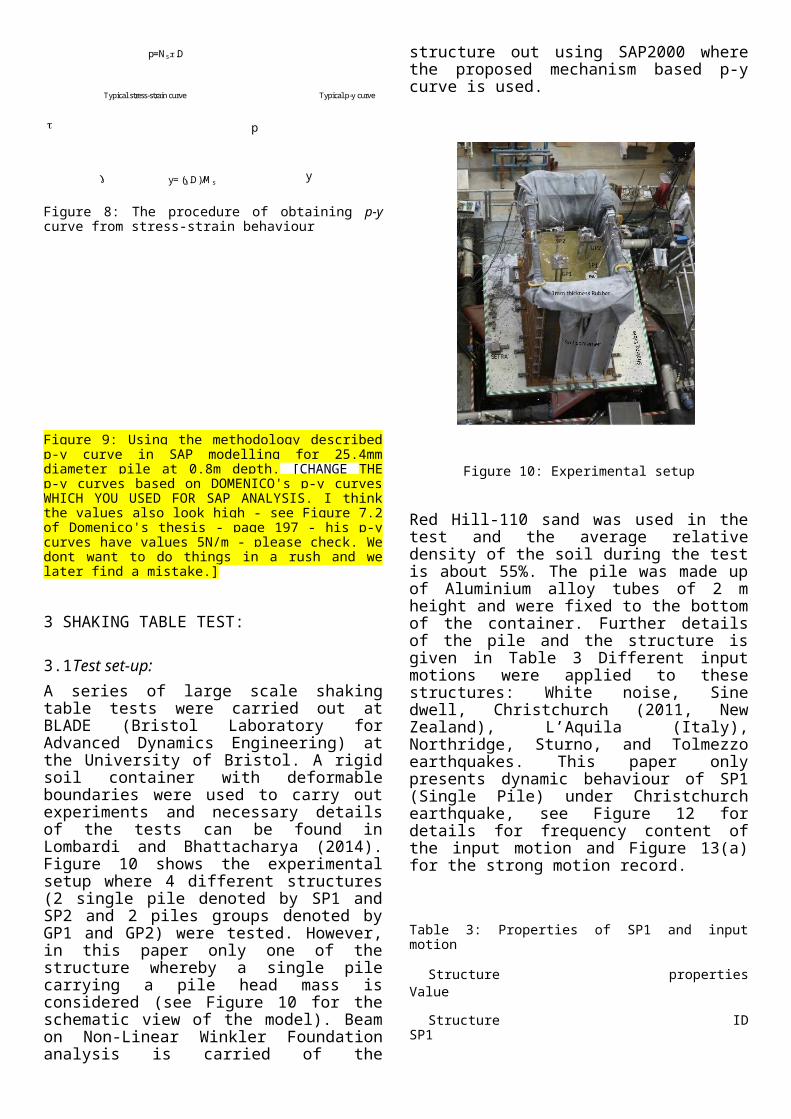
A series of large scale shaking table tests were car-ried out at BLADE (Bristol Laboratory for Ad-vanced Dynamics Engineering) at the University of Bristol. A rigid soil container with deformable boundaries were used to carry out experiments and necessary details of the tests can be found in Lom-bardi and Bhattacharya (2014). Figure 10 shows the experimental setup where 4 different structures (2 single pile denoted by SP1 and SP2 and 2 piles groups denoted by GP1 and GP2) were tested. How-ever, in this paper only one of the structure whereby a single pile carrying a pile head mass is considered (see Figure 10 for the schematic view of the model). Beam on Non-Linear Winkler Foundation analysis is carried of the structure out using SAP2000 where the proposed mechanism based p-y curve is used.
Figure 10: Experimental setup
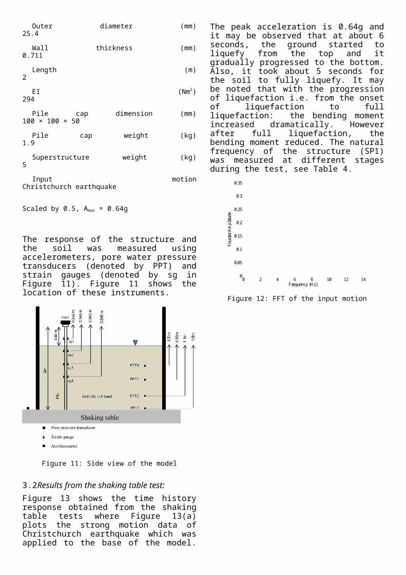
Red Hill-110 sand was used in the test and the aver-age relative density of the soil during the test is about 55%. The pile was made up of Aluminium al-loy tubes of 2 m height and were fixed to the bottom of the container. Further details of the pile and the structure is given in Table 3 Different input motions were applied to these structures: White noise, Sine dwell, Christchurch (2011, New Zealand), L’Aquila (Italy), Northridge, Sturno, and Tolmezzo earth-quakes. This paper only presents dynamic behaviour of SP1 (Single Pile) under Christchurch earthquake, see Figure 12 for details for frequency content of the input motion and Figure 13(a) for the strong motion record.
(b)
(a)
(c)
S tre ss C on tro lled
T im e (se c )
Dev
iato
r str
ess
q (k
N/m
2 )S tra in C o n tro lled
0 5 10 15 20 250
50
100
150
200
250
A x ia l s tra in (% )
Dev
iato
r st
ress
(kP
a)
R ed H ill 3 0 %
R ed H ill 5 5 %R ed H ill 7 0 %
D ecreas in gre la tiv ed en sity
y
p
Typical stress-strain curve
Typical p-y curve
p=Ns..D
y= (.D)/Ms
Table 3: Properties of SP1 and input motion
Structure properties Value
Structure ID SP1
Outer diameter (mm) 25.4
Wall thickness (mm) 0.711
Length (m) 2
EI (Nm2) 294
Pile cap dimension (mm) 100 × 100 × 50
Pile cap weight (kg) 1.9
Superstructure weight (kg) 5
Input motion Christchurch earthquake
Scaled by 0.5, Amax = 0.64g
The response of the structure and the soil was mea-sured using accelerometers, pore water pressure transducers (denoted by PPT) and strain gauges (de-noted by sg in Figure 11). Figure 11 shows the loca-tion of these instruments.
Figure 11: Side view of the model
3.2 Results from the shaking table test:
Figure 13 shows the time history response obtained from the shaking table tests where Figure 13(a) plots the strong motion data of Christchurch earthquake which was applied to the base of the model. The peak acceleration is 0.64g and it may be observed that at about 6 seconds, the ground started to liquefy from the top and it gradually progressed to the bot-tom. Also, it took about 5 seconds for the soil to fully liquefy. It may be noted that with the progres-sion of liquefaction i.e. from the onset of liquefac-
tion to full liquefaction: the bending moment in-creased dramatically. However after full liquefac-tion, the bending moment reduced. The natural fre-quency of the structure (SP1) was measured at dif-ferent stages during the test, see Table 4.
Figure 12: FFT of the input motion
0 2 4 6 8 10 12 140
0.05
0.1
0.15
0.2
0.25
0.3
0.35
Frequency (Hz)
Fou
rier
Am
plit
ude
sg 1
sg 2
sg 3
sg 4
-0 .8
-0 .4
0
0 .4
0 .8A
ccel
erat
ion
(g)
Input m otion
00 .20 .40 .60 .8
11 .2
EP
WP
R (
Ru)
Excess pore water pressure ratio (Ru)
-2 0
-1 0
0
1 0
2 0
Ben
ding
Mom
ent
(Nm
)
Bending m om ent at 0.246m from the top of the pile (sg1)
-2 0
-1 0
0
1 0
2 0
Be
ndin
g M
om
ent
(Nm
)
Bending m om ent at 0.548m from the top of the pile (sg2)
-2 0
-1 0
0
1 0
2 0
Be
ndin
g M
om
ent
(Nm
)
Bending m om ent at 0.845m from the top of the pile (sg3)
0 2 4 6 8 1 0 1 2 1 4 1 6 1 8 2 0 -2 0
-1 0
0
1 0
2 0
T im e (sec)
Be
ndin
g M
om
ent
(Nm
)
Bending m om ent at 1.297m from the top of the pile (sg4)
(d)
PPT4
PPT3
PPT2PPT1
(a)
(b)
(c)
(f)(f)
(e )
Figure 13: Time history of input motion, liquefaction and ob-served bending moment in the pile
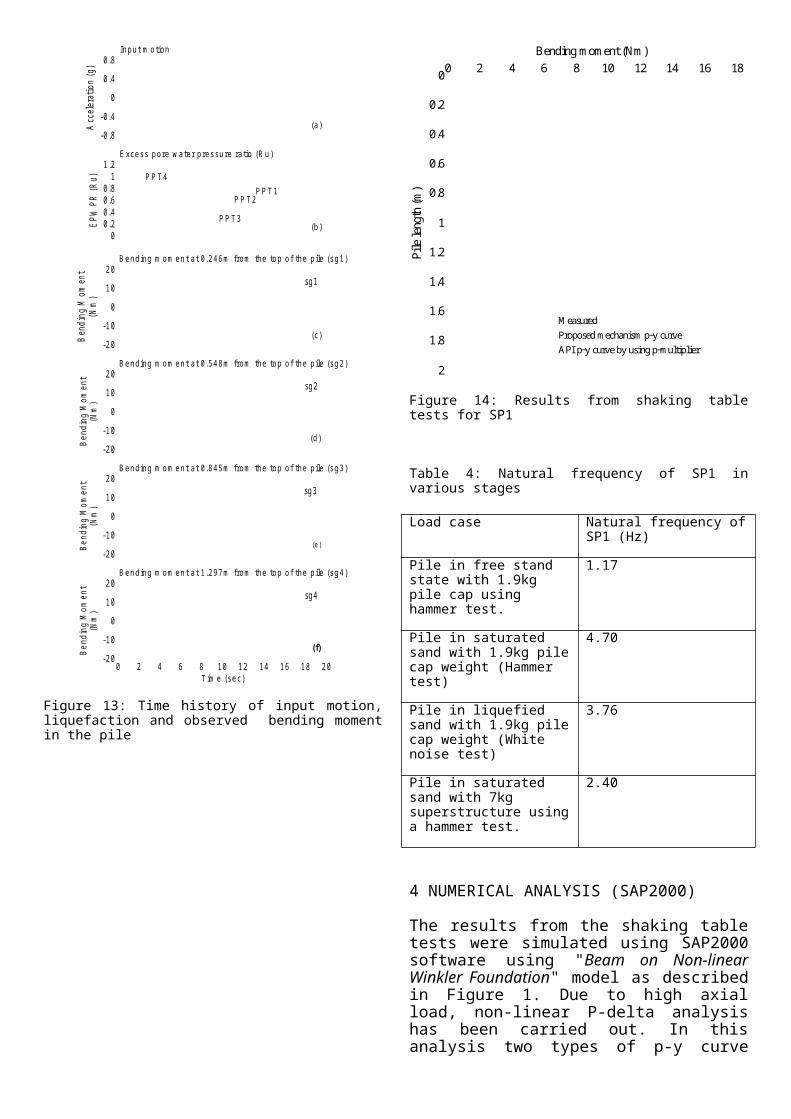
Figure 14: Results from shaking table tests for SP1
Table 4: Natural frequency of SP1 in various stages
Load case Natural frequency of SP1 (Hz)
Pile in free stand state with 1.9kg pile cap using hammer test.
1.17
Pile in saturated sand with 1.9kg pile cap weight (Ham-mer test)
4.70
Pile in liquefied sand with 1.9kg pile cap weight (White noise test)
3.76
Pile in saturated sand with 7kg superstructure using a hammer test.
2.40
4 NUMERICAL ANALYSIS (SAP2000)
The results from the shaking table tests were simu-lated using SAP2000 software using "Beam on Non-linear Winkler Foundation" model as described in Figure 1. Due to high axial load, non-linear P-delta analysis has been carried out. In this analysis two types of p-y curve have been considered: (a) p-mul-tiplier method in which standard p-y curve are multi-plied by a factor of 0.3.; (b) proposed p-y curve where there is a zero stiffness part. For the proposed p-y curves, element test results of the soil were used. Figure 14 compares the results obtained from SAP
along with the p-multiplier method and measured values. Further details of the analysis can be found in Dash et al (2010), Bhattacharya et al (2008). Few points may be noted from the results:(a) Both the p-y methods under predict the meas-ured bending moments.
5 DISCUSSION:
Figure 12 plots the FFT of the input motion and it is clear from the plot that the
Figure 13 shows different types of p-y curves for 25.4mm diameter pile and at the 0.8 m depth. As discussed earlier, the mechanism based p-y curve was derived from the stress-strain curve of liquefied soil. This type of p-y curve as well as API p-y curve multiplying to the p-multiplier were used in SAP analysis. Figure 14 shows the comparison between results of shaking table test and SAP analysis at the time of fully liquefaction. As can be seen from the figure there is difference between the amount of maximum bending moment in proposed p-y curve and experiment. This difference is due to the differ-ent applied loading. In experiment the scaled real earthquake was applied to the structure. Hence, in SAP analysis static lateral load was applied on the pile head. The obtained maximum bending moment from proposed p-y curve is around 11Nm compare to 17.5Nm from the experiment. On the other side, the achieved bending moment based on API code is dependent on the amount of p-multiplier (mp). by changing various value of mp, different amount of bending moment can be obtained.
Figure 14: Comparison the results of experiment and SAP anal-ysis
Figure 15 shows the bending moment profile of the single pile in different time of the experiment. Basi-cally, this graph consists of four stages of before liq-uefaction, transient phase, at fully liquefaction and after liquefaction. As be shown, the bending moment increases from before liquefaction to fully liquefac-tion. After liquefaction, the bending moment de-creases dramatically.
As shown in this paper, Winkler approach is the common method to analyse pile foundations. p-y curve is similar to stress strain curve of soil. The current method to obtain p-y curve for liquefiable
00 2 4 6 8 10 12 14 16 18
0.2
0.4
0.6
0.8
1
1.2
1.4
1.6
1.8
2
Bending moment (Nm)
Pil
e le
ngth
(m
)
Measured
Proposed mechanism p−y curve
API p−y curve by using p−multiplier
soils using mp may not be able to represent behavior of liquefiable soil. Therefore, a series of multi-stage cyclic triaxial tests have be carried out to obtain stress strain relationship of liquefiable soil. The pro-posed p-y curve was derived from the achieved stress strain curve. These p-y curves come from the real behavior of soil comparing to API p-y curves which is depends on reducing factor.
6 REFRENCES
American Petroleum Institute (2000). “Recommended practice for planning, designing and constracting fixed offshore platforms-Load and resistance factor design.” API-RP-2A, 21st Edition.
Bhattacharya, S., Krishna, A. M., Lombardi, D., Crewe, A. & Alexander, N. 2012. Economic MEMS based 3-axis water proof accelerometer for dynamic geo-engineering applica-tions. Soil Dynamic sand Earthquake Engineering, 36, 111-118.
Bouzid, DJ., Bhattacharya, S., Dash, SR. 2013. Winkler Springs (p-y curves) for pile design from stress-strain of soils: FE assessment of scaling coefficients using the Mo-bilized Strength Design concept. Geomechanics and Engin-eering. 5(5) 379-399.
Brandenberg, S. J. 2005. Behavior of pile foundations in lique_ed and laterally spreading ground, PhD thesis, Uni-versity of California, Davis.
Brandenberg, S. J., Boulanger, R. W., Kutter, B. L. & Chang, D. 2007. Static pushover analyses of pile groups in lique_ed and laterally spreading ground in centrifuge tests, Journal of Geotechnical and Geoenvironmental Engineer-ing.133(9), 1055-1066.
Chai, JC., Carter, JP., Hayashi, S. 2007. Modelling strain-soft-ening behavior of clayey soils. Lowland technology inter-national SI. 9(2). 29-37.
Dash, S. 2010. Lateral Pile-Soil Interaction in liquefiable Soils. PhD thesis, University of Oxford.
Dobry, R., Taboada, V. & Liu, L. 1995. Centrifuge modeling of liquefaction effects during earthquakes, in `Proc. 1st Intl. Conf. On Earthquake Geotechnical Engineering, IS-Tokyo', pp. 14-16.
Lombardi, D., Bhattacharya, S. 2014. Modal analysis of pile-supported structures during seismic liquefaction. Earth-quake Engineering & Structural Dynamic. 43:119–138.
Meyerhof, G.G. 1957. Discussion on soil properties and their measurement. In: Proc. 4th International Conference on Soil Mechanics and foundation engineering. 3.
Osman, AS., Bolton, MD. 2005. Simple plasticity-based pre-diction of the undrained settlement of shallow circular foundation on clay. Geotechnique, 55(6). 435-447.
Pan, H., Chen, G., Liu, H., Wang, B. 2011. Behaviour of large post-liquefaction deformation in saturated Nanjing fine
sand. Earthquake engineering and engineering vibration. 10(2). 187-193.
Wichtman, T. 2005. Explicit accumulation model for non-cohe-sive soils under cyclic loading, Dissertation, University of Bochum.