Router Buffer Sizing Revisited:The Role of the Output/Input Capacity Ratio

Ravi S. Prasad, Constantine Dovrolis Marina ThottanGeorgia Institute of Technology Bell-Labs{ravi, dovrolis}@cc.gatech.edu marinat@bell-labs.com

ABSTRACTThe issue of router buffer sizing is still open and significant.Previous work either considers open-loop traffic or only an-alyzes persistent TCP flows. This paper differs in two ways.First, it considers the more realistic case of non-persistentTCP flows with heavy-tailed size distribution. Second, in-stead of only looking at link metrics, we focus on the impactof buffer sizing on TCP performance. Specifically, our goalis to find the buffer size that maximizes the average per-flowTCP throughput. Through a combination of testbed experi-ments, simulation, and analysis, we reach the following con-clusions. The output/input capacity ratio at a network linklargely determines the required buffer size. If that ratio islarger than one, the loss rate drops exponentially with thebuffer size and the optimal buffer size is close to zero. Other-wise, if the output/input capacity ratio is lower than one, theloss rate follows a power-law reduction with the buffer sizeand significant buffering is needed, especially with flowsthat are mostly in congestion-avoidance. Smaller transfers,which are mostly in slow-start, require significantly smallerbuffers. We conclude by revisiting the ongoing debate on“small versus large” buffers from a new perspective.

1. INTRODUCTIONThe need for buffering is a fundamental “fact of life”

for packet switching networks. Packet buffers in routers(or switches) absorb the transient bursts that naturallyoccur in such networks, reduce the frequency of packetdrops and, especially with TCP traffic, they can avoidunder-utilization when TCP connections back off dueto packet losses. At the same time, though, buffersintroduce delay and jitter, and they increase the routercost and power dissipation.

After several decades of research and operational ex-

Permission to make digital or hard copies of all or part of this work forpersonal or classroom use is granted without fee provided that copies arenot made or distributed for profit or commercial advantage and that copiesbear this notice and the full citation on the first page. To copy otherwise, torepublish, to post on servers or to redistribute to lists, requires prior specificpermission and/or a fee.CoNEXT’ 07, December 10-13, 2007, New York, NY, U.S.A.Copyright 2007 ACM 978-1-59593-770-4/ 07/ 0012 ...$5.00.

perience with packet switching networks, it is surprisingthat we still do not know how to dimension the bufferof a router interface. As explained in detail in §2, thisbasic question - how much buffering do we need at agiven router interface? - has received hugely differentanswers in the last 15-20 years, such as “a few dozens ofpackets”, “a bandwidth-delay product”, or “a multipleof the number of large TCP flows in that link.” It can-not be that all these answers are right. It is clear thatwe are still missing a crucial piece of understanding, de-spite the apparent simplicity of the previous question.

At the same time, the issue of buffer sizing becomesincreasingly important in practice. The main reason isthat IP networks are maturing from just offering reach-ability to providing performance-centered Service-LevelAgreements and delay/loss assurances. Additionally,as the popularity of voice and video applications in-creases, the potentially negative effects of over-bufferedor under-buffered routers become more significant.

Our initial objective when we started this work wasto examine the conditions under which some previousbuffer sizing proposals hold, to identify the pros andcons of each proposal, and to reach a compromise, soto speak. In the progress of this research, however, wefound out that there is a different way to think aboutbuffer sizing, and we were led to new results and insightabout this problem.

Specifically, there are mostly three new ideas in thispaper. First, instead of assuming that most of the traf-fic consists of “persistent” TCP flows, i.e., very longtransfers that are mostly in congestion-avoidance, wework with the more realistic model of non-persistentflows that follow a heavy-tailed size distribution. Theimplications of this modeling deviation are major: first,non-persistent flows do not necessarily saturate theirpath, second, such flows can spend much of their life-time in slow-start, and third, the number of active flowsis highly variable with time. A detailed discussion onthe differences between the traffic generated from per-sistent and non-persistence flows is presented in [17].Our results show that flows which spend most of theirlifetime in slow-start require significantly less bufferingthan flows that live mostly in congestion-avoidance.

Second, instead of only considering link-level perfor-

mance metrics, such as utilization, average delay andloss probability,1 we focus on the performance of in-dividual TCP flows, and in particular, on the relationbetween the average throughput of a TCP flow and thebuffer size in its bottleneck link. TCP accounts for morethan 90% of the Internet traffic, and so a TCP-centricapproach to router buffer sizing would be appropriatein practice for both users and network operators (as-suming that the latter care about the satisfaction oftheir users/customers). On the other hand, aggregatemetrics, such as link utilization or loss probability, canhide what happens at the transport or application lay-ers. For instance, the link may have enough buffers sothat it does not suffer from under-utilization, but theper-flow TCP throughput can be abysmally low.

Third, we focus on a structural characteristic of a link(or traffic) multiplexer that has been largely ignored inthe past. This characteristic is the ratio of the out-put/input capacities. For example, consider a link ofoutput capacity Cout that receives traffic from N links,each of input capacity Cin, with NCin > Cout. In thesimplest case, where users are directly connected to theinput links, the input capacity Cin is simply the ca-pacity of those links. More generally, however, a flowcan be bottlenecked at any link between the source andthe output port under consideration. Then, Cin is thepeak rate with which a flow can arrive at the outputport. For example, consider an edge router with an out-put capacity of 10Mbps. Suppose that the input portsare 100Mbps links, but the latter aggregate traffic from1Mbps access links. In that case, the peak rate withwhich a flow can arrive at the 10Mbps output port is1Mbps, and so the ratio Cout/Cin is equal to 10.

It turns out that the ratio Γ = Cout/Cin largelydetermines the relation between loss probability andbuffer size, and consequently, the relation between TCPthroughput and buffer size. Specifically, we propose twoapproximations for the relation between buffer size andloss rate, which are reasonably accurate as long as thetraffic is heavy-tailed. If Γ < 1, the loss rate can be ap-proximated by a power-law of the buffer size. The bufferrequirement then can be significant, especially when weaim to maximize the throughput of TCP flows thatare in congestion-avoidance (the buffer requirement forTCP flows that are in slow-start is significantly lower).On the other hand, when Γ > 1, the loss probabilitydrops almost exponentially with the buffer size, andthe optimal buffer size is extremely small (just a fewpackets in practice, and zero theoretically). Usually,Γ is often lower than one in the access links of serverfarms, where hosts with 1 or 10 Gbps interfaces feedinto lower capacity edge links. On the other hand, theratio Γ is typically higher than one at the periphery ofaccess networks, as the traffic enters the high-speed corefrom limited capacity residential links.

1We use the terms loss probability and loss rate interchange-ably.

We reach the previous conclusions based on a combi-nation of experiments, simulation and analysis2. Specif-ically, after we discuss the previous work in §2, wepresent results from testbed experiments using a River-stone router (§3). These results bring up several im-portant issues, such as the importance of provisioningthe buffer size for heavy-load conditions and the exis-tence of an optimal buffer size that depends on the flowsize. The differences between large and small flows isfurther discussed in §4, where we identify two modelsfor the throughput of TCP flows, depending on whethera flow lives mostly in slow-start (S-model) or in conges-tion avoidance (L-model). As a simple analytical case-study, we use the two TCP models along with the lossprobability and queueing delay of a simple M/M/1/Bqueue to derive the optimal buffer size for this basic(but unrealistic) queue (§5).

For more realistic queueing models, we conduct anextensive simulation study in which we examine the av-erage queueing delay d(B) and loss probability p(B) asa function of the buffer size B, under heavy-load condi-tions with TCP traffic (§6). These results suggest twosimple and parsimonious empirical models for p(B). In§6 we also provide an analytical basis for the previoustwo models. In §7, we use the models for d(B) and p(B)to derive the optimal buffer size, depending on the typeof TCP flow (S-model versus L-model) and the value ofΓ. Finally, in §8, we conclude by revisiting the recentdebate on “large versus small buffers” based on the newinsight from this work.

2. RELATED WORKSeveral queueing theoretic papers analyze either the

loss probability in finite buffers, or the tail probabilityin infinite buffers. Usually, however, that modeling ap-proach considers exogenous (or open-loop) traffic mod-els, in which the packet arrival process does not dependon the state of the queue. For instance, the paper byKim and Shroff models the input traffic as a generalGaussian process, and derives an approximate expres-sion for the loss probability in a finite buffer system [11].

An early experimental study by Villamizar and Song[22] recommends that the buffer size should be equal tothe Bandwidth-Delay Product (BDP) of that link. The“delay” here refers to the RTT of a single and persistentTCP flow that attempts to saturate that link, while the“bandwidth” term refers to the capacity C of the link.No recommendations are given, however, for the morerealistic case of multiple TCP flows with different RTTs.

Appenzeller et al.[1] conclude that the buffer require-ment at a link decreases with the square root of thenumber N of “large” TCP flows that go through thatlink. According to their analysis, the buffer requirementto achieve almost full utilization is B = (CT )/

√N ,

2All experimental data and simulation scripts are availableupon request from the authors.

where T is the average RTT of the N (persistent) com-peting connections. The key insight behind this modelis that, when the number of competing flows is suffi-ciently large, which is usually the case in core links,the N flows can be considered independent and non-synchronized, and so the standard deviation of the ag-gregate offered load (and of the queue occupancy) de-

creases with√

N . An important point about this modelis that it aims to keep the utilization close to 100%,without considering the resulting loss rate.

Morris was the first to consider the loss probabilityin the buffer sizing problem [15, 16]. That work rec-ognizes that the loss rate increases with the square ofthe number of competing TCP flows, and that bufferingbased on the BDP rule can cause frequent TCP time-outs and unacceptable variations in the throughput ofcompeting transfers [15]. That work also proposes theFlow-Proportional Queueing (FPQ) mechanism, as avariation of RED, which adjusts the amount of buffer-ing proportionally to the number of TCP flows.

Dhamdhere et al. consider the buffer requirement of aDrop-Tail queue given constraints on the minimum uti-lization, maximum loss-rate, and, when feasible, max-imum queueing delay [6]. They derive the minimumbuffer size required to keep the link fully utilized by aset of N heterogeneous TCP flows, while keeping theloss rate and queueing delay bounded. However, theanalysis of that paper is also limited by the assumptionof persistent connections.

Enachescu et al. show that if the TCP sources arepaced and have a bounded maximum window size, thena high link utilization (say 80%) can be achieved evenwith a buffer of a dozen packets [8]. The authors notethat pacing may not be necessary when the access linksare much slower than the core network links. It is alsointeresting that their buffer sizing result is independentof the BDP.

Recently, the ACM CCR has hosted a debate onbuffer sizing through a sequence of letters [7, 8, 19, 23,25]. Dhamdhere and Dovrolis argue that the recent pro-posals for much smaller buffer sizes can cause significantlosses and performance degradation at the applicationlayer [7]. Similar concerns are raised by Vu-Brugier etal. in [23]. That letter also reports measurements froman operational link in which the buffer size was signif-icantly reduced. Ganjali and McKeown discuss threerecent buffer sizing proposals [1, 6, 8] and argue thatall these results may be applicable in different parts ofthe network, as they depend on various assumptionsand they have different objectives [9].

3. EXPERIMENTAL STUDYTo better understand the router buffer sizing problem

in practice, we first conducted a set of experiments in acontrolled testbed. The following results offer a numberof interesting observations. We explain these observa-tions through modeling and analysis in the following

sections.

3.1 Testbed setupThe schematic diagram of our experimental setup

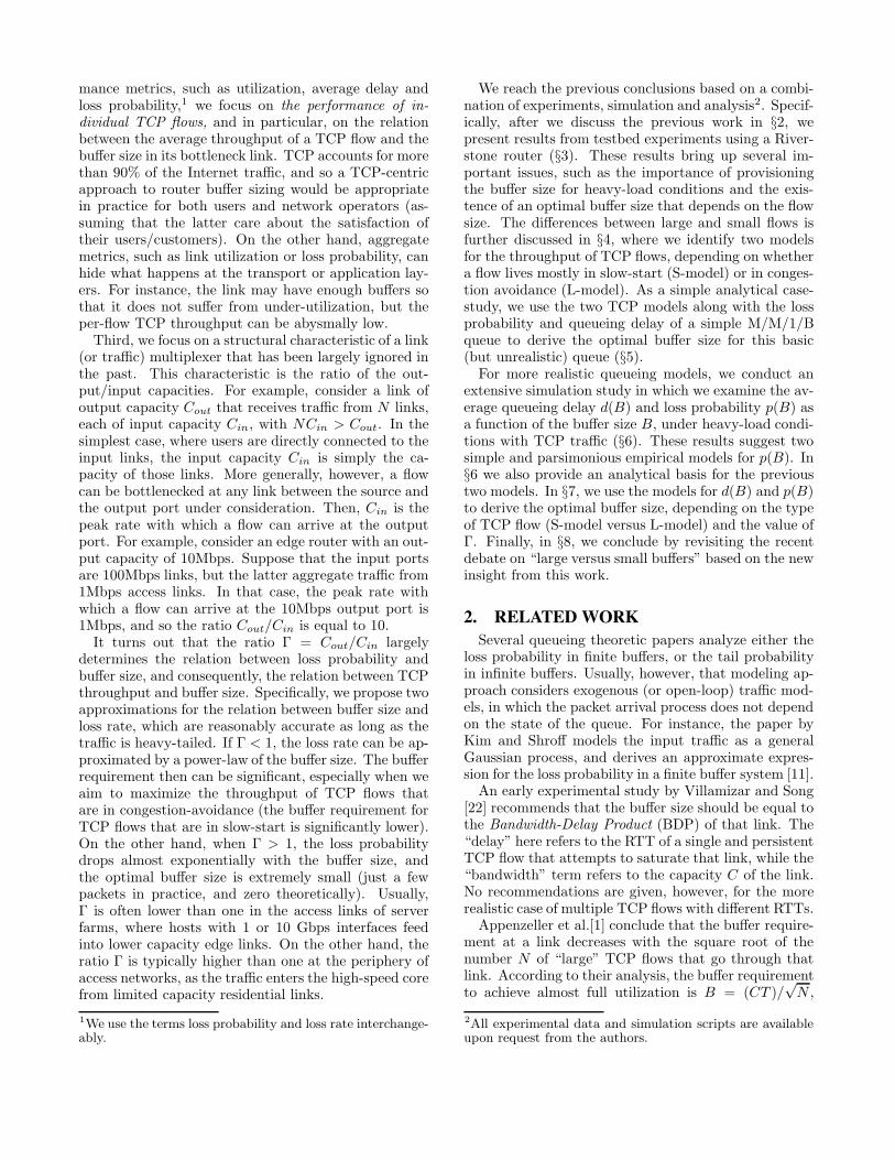
is shown in Figure 1. There are four hosts running

������������������������������������������������������������������������������������������

������������������������������������������������������������������������������������������

RiverstoneRouter1GE

1GE

Tunable Buffer

1GE

TrafficMonitor

SwitchServ

ers

Clie

nts

Switch

Switch

DelayEmulators

Figure 1: Schematic diagram of the experimen-tal testbed.

servers/senders and four hosts running clients/receivers,all of which are Fedora Core-5 Linux systems. Eachmachine has two Intel Xeon CPUs running at 3.2 GHz,2GB memory, and DLink Gigabit PCIexpress networkinterface. The traffic from four senders is aggregated ontwo Gig-Ethernet links before entering the router. Thetestbed bottleneck is the Gig-Ethernet output interfacethat connects the router to the distribution switch.

We use a Riverstone RS-15008 router. The switchingfabric has much higher capacity than the bottlenecklink, and there is no significant queueing at the inputinterfaces or at the fabric itself. The router has a tun-able buffer size at the output line card. Specifically,we experiment with 20 buffer sizes, non-uniformly se-lected in the range 30KB to 38MB. With Ethernet MTUpackets (1500B), the minimum buffer size is about 20packets while the maximum buffer size is approximately26,564 packets. We configured the output interface touse Drop-Tail 3, queueing and we confirmed that themaximum queueing delay for a buffer size B is equal toB/Cout, where Cout is the capacity of the output link.

Two delay emulators run NISTNet [4] to introducepropagation delays in the ACKs that flow from theclients to the servers. With this configuration, the min-imum RTT of the TCP connections takes one of thefollowing values, 30ms, 50ms, 120ms or 140ms, with adifferent RTT for each client machine.

We configured the Linux end-hosts to use the TCPReno stack that uses the NewReno congestion controlvariant with Selective Acknowledgments. The maxi-mum advertised TCP window size is set to 13MB, sothat transfers are never limited by that window.

The traffic is generated using the open-source Har-poon system [21]. We modified Harpoon so that it gen-erates TCP traffic in a “closed-loop” flow arrival model[20]. In this model, a given number of “users” (runningat the client hosts) performs successive TCP transfersfrom the servers. The size of TCP transfers follows agiven random distribution. After each download, the

3In this work, we use Drop-Tail queues as RED and otherAQM schemes are not widely used in the current Internet.

user stays idle for a “thinking period” that follows an-other given distribution. For the transfer sizes, we use aPareto distribution with mean 80KB and shape parame-ter 1.5. These values are realistic, based on comparisonswith actual packet traces. The think periods follow anexponential distribution with mean duration of one sec-ond. The key point, here, is that the generated traf-fic, which resembles the aggregation of many ON-OFFsources with heavy-tailed ON periods, is Long-RangeDependent (LRD) [24].

One important property of the previous closed-loopflow arrival model is that it never causes overload (i.e.,the offered load cannot exceed the capacity). If that linkbecomes congested, the transfers take longer to com-plete, and the offered load remains at or below Cout [2].Note that this is not the case in an open-loop flow ar-rival model, where new flows arrive based on an externalrandom process (e.g., a Poisson process).

We control the offered load by emulating differentnumbers of users. The three experiments that we sum-marize in this paper, referred to as U1000, U1200, andU3000, have U=1000, 1200 and 3000 users, respectively.A detailed description of the experimental setup is pre-sented in [18].

3.2 Results

3.2.1 Link utilizationFigure 2 shows the average utilization ρ of the bot-

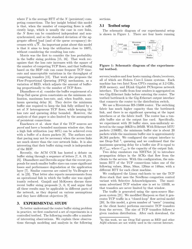
tleneck link as a function of the buffer size in each ofthe three experiments. First note that the utilizationcurves, especially in the two experiments that do notsaturate the output link, are quite noisy despite thefact that they represent 4-minute averages. Such highvariability in the offered load is typical of LRD trafficand it should be expected even in longer time scales. Weobserve that the experiment U1000 can generate an aver-age utilization of about 60-70% (with enough buffering),U1200 can generate a utilization of about 80-90%, whileU3000 can saturate the link.

10 100 1000 10000 1e+05Buffer Size (KB)

0.5

0.6

0.7

0.8

0.9

1

Link

Util

izat

ion

3000 Users1200 Users1000 Users

Figure 2: Link utilization as a function of therouter buffer size for U1000, U1200 and U3000.

Note that there is a loss of utilization when the buffersare too small. Specifically, to achieve the maximum pos-

sible utilization we need a buffer size of at least 200KBin U3000, and an even larger buffer in the other two ex-periments. The reason for the loss of utilization whenthere are not enough buffers has been studied in depthin previous work [1]. As we argue in the rest of thispaper, however, maximizing the aggregate throughputshould not be the only objective of buffer sizing.

0 10 20 30Averaging Time Scale T (sec)

0

0.05

0.1

0.15

0.2

Frac

tion

of T

ime

in H

eavy

-Loa

d

> 95%> 90%

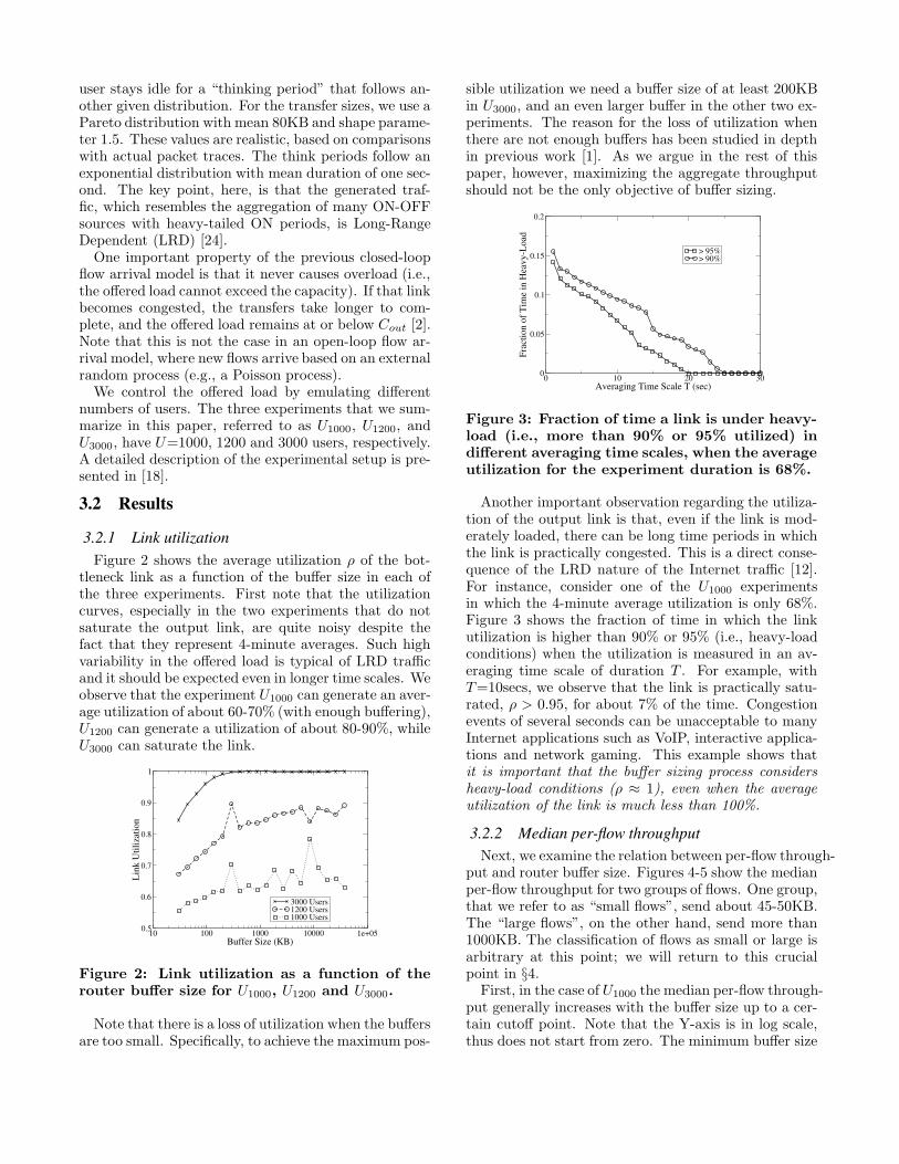
Figure 3: Fraction of time a link is under heavy-load (i.e., more than 90% or 95% utilized) indifferent averaging time scales, when the averageutilization for the experiment duration is 68%.

Another important observation regarding the utiliza-tion of the output link is that, even if the link is mod-erately loaded, there can be long time periods in whichthe link is practically congested. This is a direct conse-quence of the LRD nature of the Internet traffic [12].For instance, consider one of the U1000 experimentsin which the 4-minute average utilization is only 68%.Figure 3 shows the fraction of time in which the linkutilization is higher than 90% or 95% (i.e., heavy-loadconditions) when the utilization is measured in an av-eraging time scale of duration T . For example, withT=10secs, we observe that the link is practically satu-rated, ρ > 0.95, for about 7% of the time. Congestionevents of several seconds can be unacceptable to manyInternet applications such as VoIP, interactive applica-tions and network gaming. This example shows thatit is important that the buffer sizing process considersheavy-load conditions (ρ ≈ 1), even when the averageutilization of the link is much less than 100%.

3.2.2 Median per-flow throughputNext, we examine the relation between per-flow through-

put and router buffer size. Figures 4-5 show the medianper-flow throughput for two groups of flows. One group,that we refer to as “small flows”, send about 45-50KB.The “large flows”, on the other hand, send more than1000KB. The classification of flows as small or large isarbitrary at this point; we will return to this crucialpoint in §4.

First, in the case of U1000 the median per-flow through-put generally increases with the buffer size up to a cer-tain cutoff point. Note that the Y-axis is in log scale,thus does not start from zero. The minimum buffer size

10 100 1000 10000 1e+05Buffer Size (KB)

1000

10000M

edia

n Pe

r-flo

w T

hrou

ghpu

t (K

bps) Small flows

Large flows

Figure 4: Median per-flow throughput as a func-tion of the buffer size in the U1000 experiments.

10 100 1000 10000 1e+05Buffer Size (KB)

100

1000

10000

Med

ian

Per-f

low

Thr

ough

put (

Kbp

s) Small flowsLarge flows

Figure 5: Median per-flow throughput as a func-tion of the buffer size in the U3000 experiments.

that leads to the maximum per-flow throughput can beviewed as the optimal buffer size B̂. Note that the opti-mal buffer size is significantly lower for small flows com-pared to large flows. The experiment U1200 gives similarresults (not shown here due to space constraints). Sec-ond, the optimal buffer size for each flow type increasesas the load increases. And third, in the saturated-linkexperiment (U3000), we also note that the median per-flow throughput of small flows first increases up to amaximum point that corresponds to the optimal buffersize B̂, and it then drops to a significantly lower value.

The above experimental results raise the followingquestions: What causes the difference in the optimalbuffer size between small flows and large flows? Whydoes the per-flow throughput increase up to a certainpoint as we increase the buffer size? Why does it dropafter that point, at least for small flows? And moregenerally, what does the optimal buffer size depend on?We will answer these questions in the following sections.

4. TWO TCP THROUGHPUT MODELSThe experimental results show that there are signif-

icant differences in the per-flow throughput betweenlarge and small flows. Intuitively, one would expectthat this may have something to do with how TCP con-gestion control works. It is well known that TCP hastwo distinct modes of increasing the congestion win-

dow: either exponentially during slow-start, or linearlyduring congestion-avoidance. We also expect that mostsmall flows complete their transfers, or send most oftheir packets, during slow-start, while most large flowsswitch to congestion-avoidance at some earlier point.

102 103 1040

200

400

600

800

1000

1200

1400

1600

1800

2000

Flow Size (pkts)

Thro

ughp

ut (K

bps)

L−modelS−modelSlow−Start ModelExperiemntal

Figure 6: Average per-flow throughput as afunction of flow size for buffer size B=30KB.

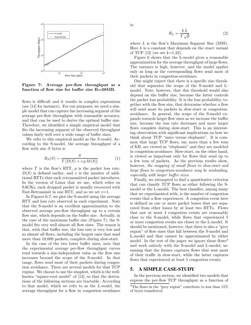
We first analyze the results of the U3000 experimentsto understand the relation between per-flow throughputand flow size. Figures 6, and 7 show this relation fortwo extreme values of the buffer size B: 30KB, and38MB. Each of the points in these graphs is the averagethroughput of all flows in a given flow size bin. The binwidth increases exponentially with the flow size (notethat the x-axis is in logarithmic scale).

These graphs show that the average throughput in-creases with the flow size, up to a certain point. Then,for the small buffer, the average throughput tends to-wards a constant value as the flow size increases (butwith high variance). How can we explain and modelthese two distinct regimes, an increasing one followedby a constant?

One may first think that the increasing segment ofthese curves can be modeled based on TCP’s slow-startbehavior. Specifically, consider a flow of size S bytes,or M(S) segments, with RTT T . If an ACK is gen-erated for every new received segment (which is thecase in the Linux 2.6.15 stack that we use), then thethroughput of a flow that completes during slow-startis approximately Rss(S) = S/[T D(S)], where D(S) =1 + dlog2(M(S)/2)e is the number of RTTs required totransfer M(S) segments during slow-start when the ini-tial window is two segments and an additional RTT isneeded for connection establishment. As we see in Fig-ure 6, however, the slow-start model significantly over-estimates the TCP throughput in the increasing phaseof the curve.

A more detailed analysis of many flows in the “smallsize” range, revealed that a significant fraction of themare subject to one or more packet losses. Even thoughit is true that they usually send most of their pack-ets during slow-start, they often also enter congestion-avoidance before completing. An exact analysis of such

102 103 104102

103

104

105

Flow Size (pkts)

Thro

ughp

ut (K

bps)

S−modelExperiemntal

Figure 7: Average per-flow throughput as afunction of flow size for buffer size B=38MB.

flows is difficult and it results in complex expressions(see [14] for instance). For our purposes, we need a sim-ple model that can capture the increasing segment of theaverage per-flow throughput with reasonable accuracy,and that can be used to derive the optimal buffer size.Therefore, we identified a simple empirical model thatfits the increasing segment of the observed throughputvalues fairly well over a wide range of buffer sizes.

We refer to this empirical model as the S-model. Ac-cording to the S-model, the average throughput of aflow with size S bytes is

RS(S) =S

T [D(S) + v p M(S)](1)

where T is the flow’s RTT, p is the packet loss rate,D(S) is defined earlier, and v is the number of addi-tional RTTs that each retransmitted packet introduces.In the version of Linux that we use, which relies onSACKs, each dropped packet is usually recovered withFast-Retransmit in one RTT, and so we set v=1.

In Figures 6-7, we plot the S-model using the averageRTT and loss rate observed in each experiment. Notethat the S-model is an excellent approximation to theobserved average per-flow throughput up to a certainflow size, which depends on the buffer size. Actually, inthe case of the maximum buffer size (Figure 7), the S-model fits very well almost all flow sizes. The reason isthat, with that buffer size, the loss rate is very low andso almost all flows, including the largest ones that sendmore than 10,000 packets, complete during slow-start.

In the case of the two lower buffer sizes, note thatthe experimental average per-flow throughput curvestend towards a size-independent value as the flow sizeincreases beyond the scope of the S-model. In thatrange, flows send most of their packets during conges-tion avoidance. There are several models for that TCPregime. We choose to use the simplest, which is the well-known “square-root model” of [13], so that the deriva-tions of the following sections are tractable. Accordingto that model, which we refer to as the L-model, theaverage throughput for a flow in congestion avoidance

is:

RL =k L

T√

p(2)

where L is the flow’s Maximum Segment Size (MSS).Here k is a constant that depends on the exact variantof TCP [13] (we set k=1.22).

Figure 6 shows that the L-model gives a reasonableapproximation for the average throughput of large flows.The variance is high, however, and the model appliesonly as long as the corresponding flows send most oftheir packets in congestion-avoidance.

One might expect that there is a specific size thresh-old that separates the scope of the S-model and L-model. Note, however, that this threshold would alsodepend on the buffer size, because the latter controlsthe packet loss probability. It is the loss probability, to-gether with the flow size, that determine whether a flowwill send most its packets in slow-start or congestion-avoidance. In general, the scope of the S-model ex-pands towards larger flow sizes as we increase the buffersize, because the loss rate decreases and more largerflows complete during slow-start. This is an interest-ing observation with significant implications on how wethink about TCP “mice versus elephants”. It is com-mon that large TCP flows, say more than a few tensof KB, are viewed as “elephants” and they are modeledin congestion-avoidance. Slow-start, on the other hand,is viewed as important only for flows that send up toa few tens of packets. As the previous results show,however, the mapping of small flows to slow-start andlarge flows to congestion-avoidance may be misleading,especially with larger buffer sizes.

Finally, we attempted to find a quantitative criterionthat can classify TCP flows as either following the S-model or the L-model. The best classifier, among manythat we experimented with, is the number of congestionevents that a flow experiences. A congestion event hereis defined as one or more packet losses that are sepa-rated from other losses by at least two RTTs. Flowsthat saw at most 4 congestion events are reasonablyclose to the S-model, while flows that experienced 5or more congestion events are closer to the L-model. Itshould be mentioned, however, that there is also a “greyregion” of flow sizes that fall between the S-model andL-model and that cannot be approximated by eithermodel. In the rest of the paper we ignore those flows4

and work entirely with the S-model and L-model, as-suming that the former captures flows that sent mostof their traffic in slow-start, while the latter capturesflows that experienced at least 5 congestion events.

5. A SIMPLE CASE-STUDYIn the previous section, we identified two models that

express the per-flow TCP throughput as a function of4The flows in the “grey region” contribute to less than 15%of bytes transferred.

the loss probability and RTT that the flow experiencesin its path. In this section, we consider a TCP flow ofsize S that goes through a single bottleneck link. Thelink has capacity C and B packet buffers. Our goal is tofirst derive the throughput R(B) of the flow as a func-tion of the buffer size at the bottleneck link, and then tocalculate the buffer size that maximizes the throughputR(B). To do so, we need to know the loss probabilityp(B) and average queueing delay d(B) as a function ofB. As a simple case-study, even if it is not realistic, weconsider the M/M/1/B queueing model. Further, wefocus on heavy-load conditions, when the link utiliza-tion is close to 100% for the two reasons we explained in§3: first, a closed-loop flow arrival model cannot gener-ate overload, and second, the LRD nature of the trafficimplies that there will be significant time periods ofheavy-load even if the long-term average utilization ismuch less than 100%.

In the M/M/1/B model, the loss probability is given

by, p(ρ, B) = (1−ρ)ρB

1−ρB+1 . In the heavy-load regime, as ρ

tends to 1, the loss probability becomes simply inverselyproportional to the number of packet buffers p(B) =1/B. The average queueing delay, in the heavy-loadregime, becomes d(B) = B/(2C). The RTT of the TCPflow we consider can then be written as T = To+B/2C,where To is the RTT of the flow excluding the queueingdelays in the bottleneck link.

We can now substitute the previous expressions forthe loss rate and RTT in the throughput equations forthe S-model and L-model, (1) and (2), to derive the av-erage throughput R(B) as a function of the buffer size.Figure 8 shows the throughput R(B) for the S-model

101 102 103 104 1050

200

400

600

800

1000

1200

1400

Buffer Size (KB)

Thro

ughp

ut (K

bps)

S−model

L−model

Figure 8: Average throughput as a function ofthe router buffer size when the loss rate andthe average queueing delay are given by theM/M/1/B equations in the heavy-load regime.

and the L-model, in the case of a link with C = 1Gbpsand of a flow with To = 60ms and S=30pkts=45KB.Note that both TCP models have an optimal buffer sizeB̂ at which the throughput is maximized.

The initial throughput increase as we increase B canbe attributed to the significant reduction in the lossprobability. Near the optimal buffer size, the gain in

throughput due to loss probability reduction is offset byan increase in the queueing delay. Beyond the optimalbuffer size the effect of the increasing queueing delaysdominates, and the throughput is reduced in both theL-model and S-model. Further, note the optimal buffersize is much lower in the S-model case.

It is straightforward to derive the optimal buffer sizeB̂S and B̂L for the S-model and the L-model, respec-tively:

B̂S =

√

2vM(S)

D(S)CTo (3)

B̂L = 2CTo, (4)

Interestingly, the optimal buffer size for the L-model issimply twice the bandwidth-delay product (BDP). Onthe other hand, the optimal buffer size for the S-modelincreases with the square-root of the BDP. This explainswhy the smaller flows that we considered in the exper-imental results have a lower optimal buffer size thanthe larger flows. For example, the optimal buffer sizeat a 1Gbps link with To=60ms (BDP: CTo=7.5MB)is, first according to the S-model, 0.03CTo (225KB) forS=10KB, 0.06CTo (450KB) for S=100KB, and 0.15CTo

(1.125MB) for S=1MB. According to the L-model, onthe other hand, the optimal buffer size is 2CTo, whichis equal to 15MB!

Clearly, the optimal buffer size at a network linkheavily depends on whether the link is optimized forsmaller flows that typically send most of their traffic inslow-start, or for bulk transfers that mostly live in con-gestion avoidance. From the network operator’s per-spective, it would be better if all flows followed theS-model so that routers could also have much smallerbuffering requirements.

6. DELAY AND LOSS IN HEAVY LOADIn the previous section, we derived closed-form ex-

pressions for the per-flow throughput R(B) as a func-tion of the buffer size for the simplistic case of theM/M/1/B model. Of course in reality packets do notarrive based on a Poisson process and they do not haveexponentially distributed sizes. Instead, the packet in-terarrival process exhibits significant correlations andburstiness even in highly multiplexed traffic [10, 12].

In this section, we aim to address the following ques-tion: In the heavy-load regime (ρ ≈ 1), are there simplefunctional forms for p(B) and d(B) that are reason-ably accurate for LRD TCP traffic across a wide rangeof output/input capacity ratios and degrees of statisticalmultiplexing? Given that the exact expressions for p(B)and d(B) could depend on several parameters that de-scribe the input traffic and multiplexer characteristics,here we focus on “functional forms”, i.e., on general ex-pressions for these two functions, without attempting toderive the exact dependencies between the involved pa-rameters and p(B) or d(B). For instance, a functional

form for the loss rate could be of the form p(B) = a B−b,for some unknown parameters a and b. Recall that thereason we focus on the heavy-load regime is due to theLRD nature of the traffic: even if the long-term utiliza-tion is moderate, there will be significant time periodswhere the utilization will be close to 100%.

The mathematical analysis of queues with finite buffersis notoriously hard, even for simple traffic models. Forinstance, there is no closed-form expression for the lossrate in the simple case of the M/D/1/B model [3]. Evenasymptotic analysis (as B tends to infinity) is hard forarbitrary load conditions and general traffic models. Onthe other hand, it is often the case that good empiricalapproximations do exist in the heavy-load regime. Forinstance, see the Allen-Cunneen formula for the averagequeueing delay in the G/G/1 model [3].

The approach that we follow in this section is largelyempirical and it is based, first, on extensive simulations,and second, on analytical reasoning. In particular, weexamine whether we can approximate p(B) and d(B)by parsimonious functional forms in heavy-load condi-tions. The main conclusions of the following study aresummarized as follows. The queueing delay d(B) can beapproximated as linearly increasing with B (up to a cer-tain cutoff point that depends on the maximum offeredload) and the loss rate p(B) can be approximated as de-creasing exponentially with B (i.e., p(B) ≈ ae−bB) or asa power-law of B (i.e., p(B) ≈ aB−b), depending on theoutput/input capacity ratio. Next, § 6.1 shows some ofthe simulation results that led us to these conclusions,while § 6.2 provides an analytical basis for these modelsand for the conditions under which they hold.

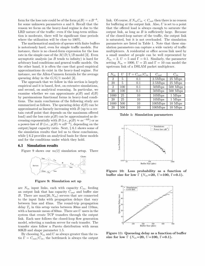
6.1 Simulation resultsFigure 9 shows our ns(2) simulation setup. There

C

CB

Clients1

2

1

25ms

45ms

5ms

5ms

in

out

UNin

Servers

Figure 9: Simulation set up

are Nin input links, each with capacity Cin, feedingan output link that has capacity Cout and buffer sizeB. There are max(20, Nin) servers that are connectedto the input links with propagation delays that varybetween 5ms and 45ms. The round-trip propagationdelay To in this setup varies between 30ms and 110ms,with a harmonic mean of 60ms. There are U users in thesystem that create TCP transfers through the outputlink. Each user follows the closed-loop flow generationmodel, selecting a random server for each transfer. Thetransfer sizes follow a Pareto distribution with mean80KB and shape parameter 1.5.

By choosing Nin and U as always greater than the ra-tio Γ = Cout/Cin, the bottleneck is always the output

link. Of course, if NinCin < Cout then there is no reasonfor buffering at the output link. Also, U is set to a pointthat the offered load is always enough to saturate theoutput link, as long as B is sufficiently large. Becauseof the closed-loop nature of the traffic, the output linkis saturated, but it is not overloaded. The simulationparameters are listed in Table 1. Note that these sim-ulation parameters can capture a wide variety of trafficmultiplexers. A residential or office access link used bya small number of people can be well represented byNin = 2, U = 5 and Γ = 0.1. Similarly, the parametersetting Nin = 1000, U = 25 and Γ = 10 can model theupstream link of a DSLAM packet multiplexer.

Nin U Γ = Cout/Cin Cout Cin

2 5 0.1 2.5Mbps 25 Mbps20 5 0.1 2.5Mbps 25 Mbps2 100 0.1 50Mbps 500 Mbps20 100 0.1 50Mbps 500 Mbps

1000 25 10 10Mbps 1 Mbps20 25 10 10Mbps 1 Mbps

1000 500 10 100Mbps 10 Mbps20 500 10 100Mbps 10 Mbps

Table 1: Simulation parameters

10 100 1000Buffer Size (pkts)

0.01

0.1

Loss

Pro

babi

lity

SimulationsPower law (aB-b)

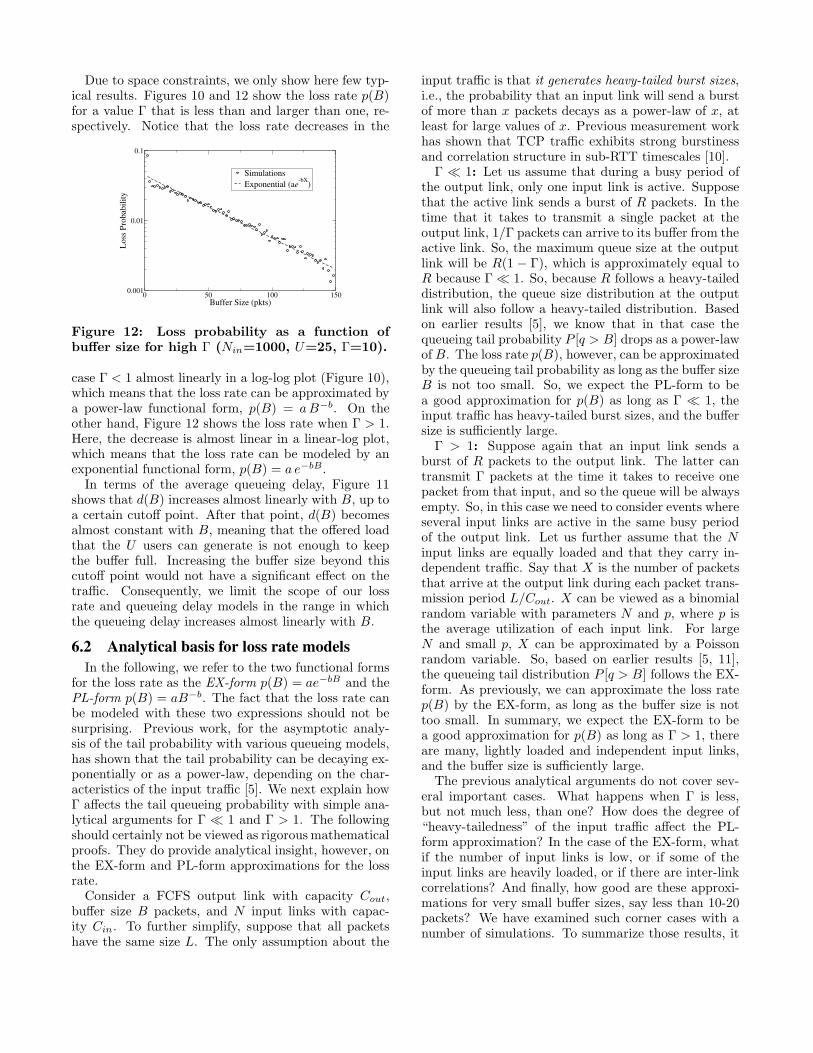
Figure 10: Loss probability as a function ofbuffer size for low Γ (Nin=20, U=100, Γ=0.1).

0 100 200 300 400 500Buffer Size (pkts)

0

10

20

30

40

50

60

Que

uein

g D

elay

(ms)

Simulations0.454 B/C

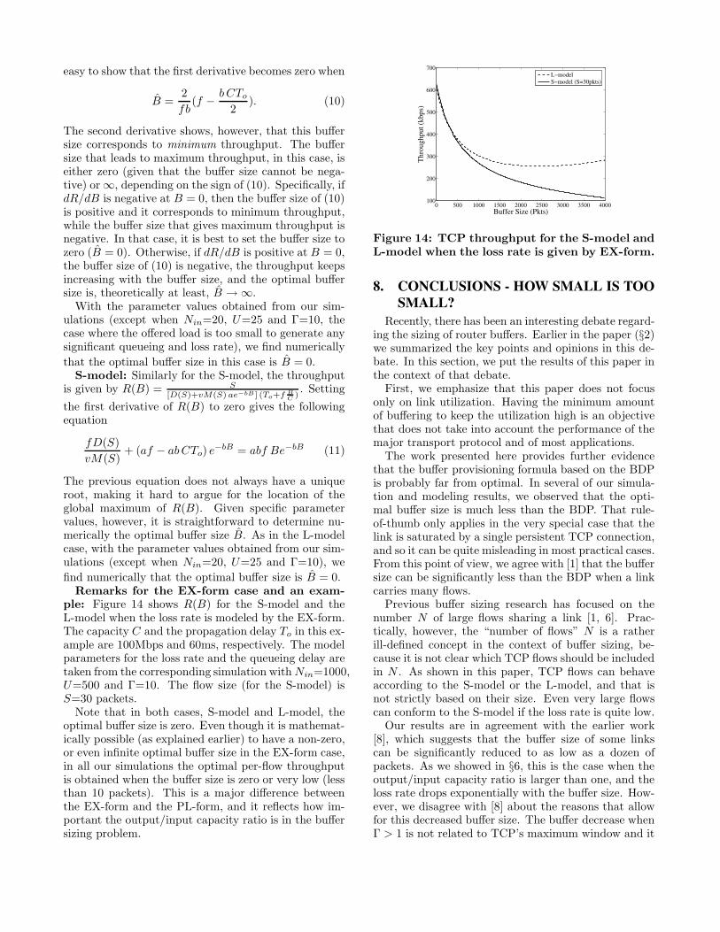
Figure 11: Queueing delay as a function of buffersize for low Γ (Nin=20, U=100, Γ=0.1).

Due to space constraints, we only show here few typ-ical results. Figures 10 and 12 show the loss rate p(B)for a value Γ that is less than and larger than one, re-spectively. Notice that the loss rate decreases in the

0 50 100 150Buffer Size (pkts)

0.001

0.01

0.1

Loss

Pro

babi

lity

SimulationsExponential (ae-bX)

Figure 12: Loss probability as a function ofbuffer size for high Γ (Nin=1000, U=25, Γ=10).

case Γ < 1 almost linearly in a log-log plot (Figure 10),which means that the loss rate can be approximated bya power-law functional form, p(B) = a B−b. On theother hand, Figure 12 shows the loss rate when Γ > 1.Here, the decrease is almost linear in a linear-log plot,which means that the loss rate can be modeled by anexponential functional form, p(B) = a e−bB.

In terms of the average queueing delay, Figure 11shows that d(B) increases almost linearly with B, up toa certain cutoff point. After that point, d(B) becomesalmost constant with B, meaning that the offered loadthat the U users can generate is not enough to keepthe buffer full. Increasing the buffer size beyond thiscutoff point would not have a significant effect on thetraffic. Consequently, we limit the scope of our lossrate and queueing delay models in the range in whichthe queueing delay increases almost linearly with B.

6.2 Analytical basis for loss rate modelsIn the following, we refer to the two functional forms

for the loss rate as the EX-form p(B) = ae−bB and thePL-form p(B) = aB−b. The fact that the loss rate canbe modeled with these two expressions should not besurprising. Previous work, for the asymptotic analy-sis of the tail probability with various queueing models,has shown that the tail probability can be decaying ex-ponentially or as a power-law, depending on the char-acteristics of the input traffic [5]. We next explain howΓ affects the tail queueing probability with simple ana-lytical arguments for Γ � 1 and Γ > 1. The followingshould certainly not be viewed as rigorous mathematicalproofs. They do provide analytical insight, however, onthe EX-form and PL-form approximations for the lossrate.

Consider a FCFS output link with capacity Cout,buffer size B packets, and N input links with capac-ity Cin. To further simplify, suppose that all packetshave the same size L. The only assumption about the

input traffic is that it generates heavy-tailed burst sizes,i.e., the probability that an input link will send a burstof more than x packets decays as a power-law of x, atleast for large values of x. Previous measurement workhas shown that TCP traffic exhibits strong burstinessand correlation structure in sub-RTT timescales [10].

Γ � 1: Let us assume that during a busy period ofthe output link, only one input link is active. Supposethat the active link sends a burst of R packets. In thetime that it takes to transmit a single packet at theoutput link, 1/Γ packets can arrive to its buffer from theactive link. So, the maximum queue size at the outputlink will be R(1 − Γ), which is approximately equal toR because Γ � 1. So, because R follows a heavy-taileddistribution, the queue size distribution at the outputlink will also follow a heavy-tailed distribution. Basedon earlier results [5], we know that in that case thequeueing tail probability P [q > B] drops as a power-lawof B. The loss rate p(B), however, can be approximatedby the queueing tail probability as long as the buffer sizeB is not too small. So, we expect the PL-form to bea good approximation for p(B) as long as Γ � 1, theinput traffic has heavy-tailed burst sizes, and the buffersize is sufficiently large.

Γ > 1: Suppose again that an input link sends aburst of R packets to the output link. The latter cantransmit Γ packets at the time it takes to receive onepacket from that input, and so the queue will be alwaysempty. So, in this case we need to consider events whereseveral input links are active in the same busy periodof the output link. Let us further assume that the Ninput links are equally loaded and that they carry in-dependent traffic. Say that X is the number of packetsthat arrive at the output link during each packet trans-mission period L/Cout. X can be viewed as a binomialrandom variable with parameters N and p, where p isthe average utilization of each input link. For largeN and small p, X can be approximated by a Poissonrandom variable. So, based on earlier results [5, 11],the queueing tail distribution P [q > B] follows the EX-form. As previously, we can approximate the loss ratep(B) by the EX-form, as long as the buffer size is nottoo small. In summary, we expect the EX-form to bea good approximation for p(B) as long as Γ > 1, thereare many, lightly loaded and independent input links,and the buffer size is sufficiently large.

The previous analytical arguments do not cover sev-eral important cases. What happens when Γ is less,but not much less, than one? How does the degree of“heavy-tailedness” of the input traffic affect the PL-form approximation? In the case of the EX-form, whatif the number of input links is low, or if some of theinput links are heavily loaded, or if there are inter-linkcorrelations? And finally, how good are these approxi-mations for very small buffer sizes, say less than 10-20packets? We have examined such corner cases with anumber of simulations. To summarize those results, it

appears that the EX-form is quite robust as long asΓ > 1. On the other hand, the PL-form is not anacceptable approximation when Γ is less but close toone and the input traffic is not strongly heavy-tailed.In that case, neither the PL-form nor the EX-form areparticularly good approximations.

7. OPTIMAL BUFFER SIZEIn the previous section, we proposed functional forms

for the average queueing delay and loss rate. The formeris a linear function of the buffer size, d(B) = fB/C, upto a certain point determined by the maximum offeredload. The latter is either the EX-form p(B) = ae−bB orthe PL-form p(B) = aB−b. In this section, we deriveexpressions for (1) the average per-flow TCP through-put R(B) as a function of the buffer size in the heavy-

load regime, and (2) the optimal buffer size B̂, i.e., thevalue of B that maximizes the average per-flow TCPthroughput. These expressions are derived for bothTCP throughput models (L-model and S-model) andfor both loss rate forms (EX-form and PL-form).

7.1 PL-formFirst, we consider the case that the loss rate decreases

as a power-law of the buffer size,

p(B) = a B−b (5)

where a and b are positive constants. The queueingdelay is modeled by a linear function, and so the RTTT (B) is given by

T (B) = To + fB

C(6)

where To is the round-trip propagation delay (excludingqueueing delays) at the bottleneck link, C is the outputlink capacity, and f is a positive constant.

L-model: In the L-model, the throughput R(B) isgiven by R(B) = kL

√

aB−b (To+f B

C). After setting the

derivative of R(B) to zero we find out that the opti-

mal buffer size B̂ is:

B̂ =b

f(2 − b)CTo (7)

The second derivative confirms that this is indeed amaximum.

Equation (7) shows that the maximum per-flow through-put is positive when b < 2. In our simulations, weobserved that this is always the case, and that typicalvalues for b and f are around 0.5 and 0.4, respectively.This makes B̂ approximately 0.83CTo. Also note thatthe optimal buffer size is independent of the parametera. What determines the value of B̂ is the rate b at whichthe loss rate decays with B, rather than the absolutevalue of the loss rate.

S-model: In the S-model, the throughput R(B) isgiven by R(B) = S

[D(S)+v M(S) a B−b] (To+f B

C), where

D(S), v, and M(S) are the previously defined S-modelparameters for a flow of size S. In the following, we setv = 1 (as discussed in §4).

Again, after calculating the first two derivatives, wefind that the optimal buffer size B̂ is the solution of thefollowing equation:

[ab M(S) CTo] B−(1+b) = a M(S) f(1− b) B−b + fD(S)

(8)Unfortunately, we do not have a closed-form solutionfor this equation. With the parameter values that re-sult from our simulations, however, we observed thatits numerical solution is always positive.

Remarks for the PL-form case and an exam-ple: For the M/M/1/B model under heavy-load, theloss rate conforms to the PL-form with a = 1 and b = 1,and the delay coefficient is f = 1/2. For these param-

eter values, (7) reduces to B̂ = 2CTo, while (8) gives

B̂ =√

2M(S)D(S) C To. These are the same expressions we

derived in §5.

0 200 400 600 800 1000300

400

500

600

700

800

900

1000

1100

Buffer Size (pkts)

Thro

ughp

ut (k

bps)

L−modelS−model (S=30pkts)

Figure 13: TCP throughput for the S-model andL-model when the loss rate is given by PL-form.

Figure 13 shows R(B) for the S-model and the L-model when the loss rate is modeled by the PL-form.The capacity C and the propagation delay To in thisexample are 50Mbps and 60ms, respectively. The modelparameters for the loss rate and the queueing delay aretaken from the simulation with Nin=20, U=100 andΓ=0.1. The flow size (for the S-model) is S=30 packets.Note that the optimal buffer size with the S-model issignificantly lower than with the L-model (about 100packets versus 400 packets, respectively).

7.2 EX-formIn this case, the loss rate p(B) is given by

p(B) = ae−bB (9)

where a and b are positive constants and the RTT T (B)is again given by (6).

L-model: The per-flow throughput for the L-modelunder the EX-form is R(B) = kL

√

ae−bB (To+f B

C). It is

easy to show that the first derivative becomes zero when

B̂ =2

fb(f − b CTo

2). (10)

The second derivative shows, however, that this buffersize corresponds to minimum throughput. The buffersize that leads to maximum throughput, in this case, iseither zero (given that the buffer size cannot be nega-tive) or ∞, depending on the sign of (10). Specifically, ifdR/dB is negative at B = 0, then the buffer size of (10)is positive and it corresponds to minimum throughput,while the buffer size that gives maximum throughput isnegative. In that case, it is best to set the buffer size tozero (B̂ = 0). Otherwise, if dR/dB is positive at B = 0,the buffer size of (10) is negative, the throughput keepsincreasing with the buffer size, and the optimal buffersize is, theoretically at least, B̂ → ∞.

With the parameter values obtained from our sim-ulations (except when Nin=20, U=25 and Γ=10, thecase where the offered load is too small to generate anysignificant queueing and loss rate), we find numerically

that the optimal buffer size in this case is B̂ = 0.S-model: Similarly for the S-model, the throughput

is given by R(B) = S

[D(S)+vM(S) ae−bB ] (To+f B

C). Setting

the first derivative of R(B) to zero gives the followingequation

fD(S)

vM(S)+ (af − ab CTo) e−bB = abf Be−bB (11)

The previous equation does not always have a uniqueroot, making it hard to argue for the location of theglobal maximum of R(B). Given specific parametervalues, however, it is straightforward to determine nu-merically the optimal buffer size B̂. As in the L-modelcase, with the parameter values obtained from our sim-ulations (except when Nin=20, U=25 and Γ=10), we

find numerically that the optimal buffer size is B̂ = 0.Remarks for the EX-form case and an exam-

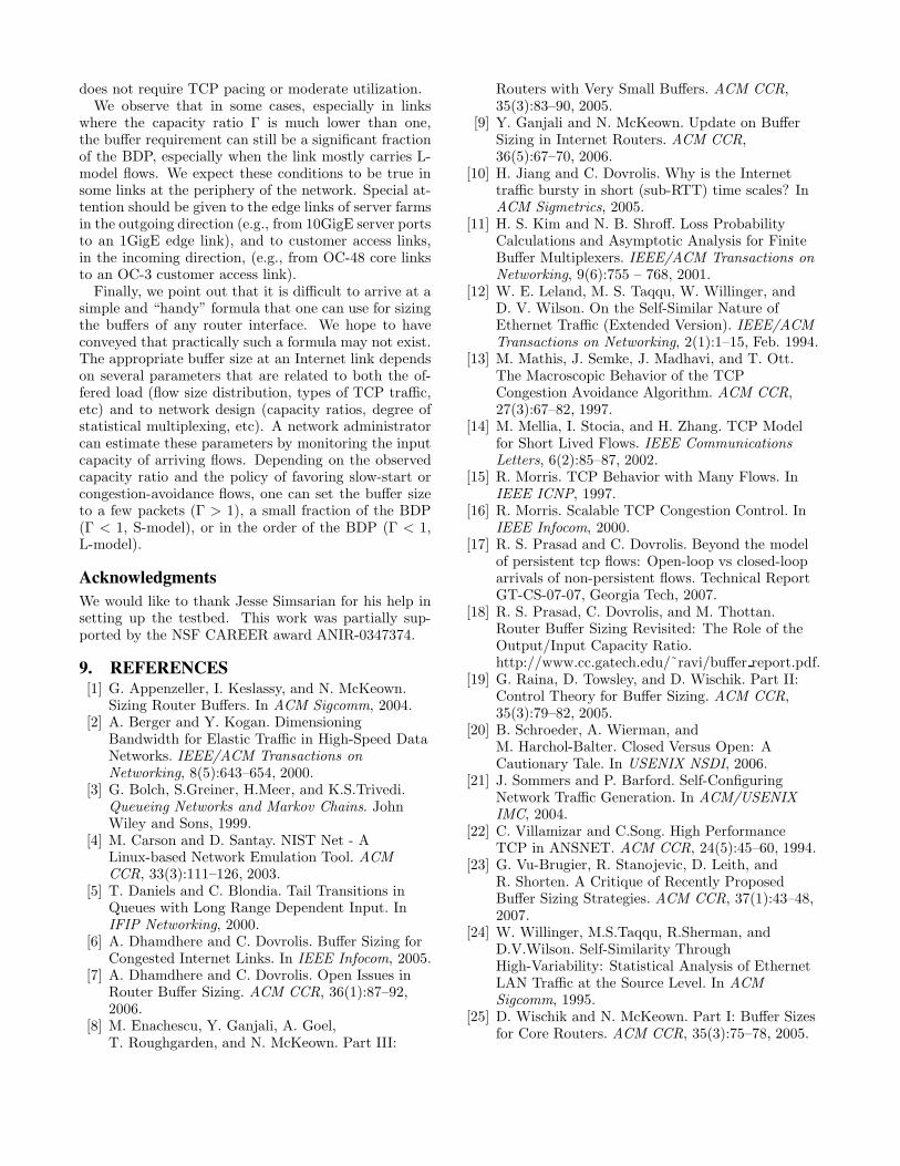
ple: Figure 14 shows R(B) for the S-model and theL-model when the loss rate is modeled by the EX-form.The capacity C and the propagation delay To in this ex-ample are 100Mbps and 60ms, respectively. The modelparameters for the loss rate and the queueing delay aretaken from the corresponding simulation with Nin=1000,U=500 and Γ=10. The flow size (for the S-model) isS=30 packets.

Note that in both cases, S-model and L-model, theoptimal buffer size is zero. Even though it is mathemat-ically possible (as explained earlier) to have a non-zero,or even infinite optimal buffer size in the EX-form case,in all our simulations the optimal per-flow throughputis obtained when the buffer size is zero or very low (lessthan 10 packets). This is a major difference betweenthe EX-form and the PL-form, and it reflects how im-portant the output/input capacity ratio is in the buffersizing problem.

0 500 1000 1500 2000 2500 3000 3500 4000100

200

300

400

500

600

700

Buffer Size (Pkts)

Thro

ughp

ut (k

bps)

L−modelS−model (S=30pkts)

Figure 14: TCP throughput for the S-model andL-model when the loss rate is given by EX-form.

8. CONCLUSIONS - HOW SMALL IS TOOSMALL?

Recently, there has been an interesting debate regard-ing the sizing of router buffers. Earlier in the paper (§2)we summarized the key points and opinions in this de-bate. In this section, we put the results of this paper inthe context of that debate.

First, we emphasize that this paper does not focusonly on link utilization. Having the minimum amountof buffering to keep the utilization high is an objectivethat does not take into account the performance of themajor transport protocol and of most applications.

The work presented here provides further evidencethat the buffer provisioning formula based on the BDPis probably far from optimal. In several of our simula-tion and modeling results, we observed that the opti-mal buffer size is much less than the BDP. That rule-of-thumb only applies in the very special case that thelink is saturated by a single persistent TCP connection,and so it can be quite misleading in most practical cases.From this point of view, we agree with [1] that the buffersize can be significantly less than the BDP when a linkcarries many flows.

Previous buffer sizing research has focused on thenumber N of large flows sharing a link [1, 6]. Prac-tically, however, the “number of flows” N is a ratherill-defined concept in the context of buffer sizing, be-cause it is not clear which TCP flows should be includedin N . As shown in this paper, TCP flows can behaveaccording to the S-model or the L-model, and that isnot strictly based on their size. Even very large flowscan conform to the S-model if the loss rate is quite low.

Our results are in agreement with the earlier work[8], which suggests that the buffer size of some linkscan be significantly reduced to as low as a dozen ofpackets. As we showed in §6, this is the case when theoutput/input capacity ratio is larger than one, and theloss rate drops exponentially with the buffer size. How-ever, we disagree with [8] about the reasons that allowfor this decreased buffer size. The buffer decrease whenΓ > 1 is not related to TCP’s maximum window and it

does not require TCP pacing or moderate utilization.We observe that in some cases, especially in links

where the capacity ratio Γ is much lower than one,the buffer requirement can still be a significant fractionof the BDP, especially when the link mostly carries L-model flows. We expect these conditions to be true insome links at the periphery of the network. Special at-tention should be given to the edge links of server farmsin the outgoing direction (e.g., from 10GigE server portsto an 1GigE edge link), and to customer access links,in the incoming direction, (e.g., from OC-48 core linksto an OC-3 customer access link).

Finally, we point out that it is difficult to arrive at asimple and “handy” formula that one can use for sizingthe buffers of any router interface. We hope to haveconveyed that practically such a formula may not exist.The appropriate buffer size at an Internet link dependson several parameters that are related to both the of-fered load (flow size distribution, types of TCP traffic,etc) and to network design (capacity ratios, degree ofstatistical multiplexing, etc). A network administratorcan estimate these parameters by monitoring the inputcapacity of arriving flows. Depending on the observedcapacity ratio and the policy of favoring slow-start orcongestion-avoidance flows, one can set the buffer sizeto a few packets (Γ > 1), a small fraction of the BDP(Γ < 1, S-model), or in the order of the BDP (Γ < 1,L-model).

AcknowledgmentsWe would like to thank Jesse Simsarian for his help insetting up the testbed. This work was partially sup-ported by the NSF CAREER award ANIR-0347374.

9. REFERENCES[1] G. Appenzeller, I. Keslassy, and N. McKeown.

Sizing Router Buffers. In ACM Sigcomm, 2004.[2] A. Berger and Y. Kogan. Dimensioning

Bandwidth for Elastic Traffic in High-Speed DataNetworks. IEEE/ACM Transactions onNetworking, 8(5):643–654, 2000.

[3] G. Bolch, S.Greiner, H.Meer, and K.S.Trivedi.Queueing Networks and Markov Chains. JohnWiley and Sons, 1999.

[4] M. Carson and D. Santay. NIST Net - ALinux-based Network Emulation Tool. ACMCCR, 33(3):111–126, 2003.

[5] T. Daniels and C. Blondia. Tail Transitions inQueues with Long Range Dependent Input. InIFIP Networking, 2000.

[6] A. Dhamdhere and C. Dovrolis. Buffer Sizing forCongested Internet Links. In IEEE Infocom, 2005.

[7] A. Dhamdhere and C. Dovrolis. Open Issues inRouter Buffer Sizing. ACM CCR, 36(1):87–92,2006.

[8] M. Enachescu, Y. Ganjali, A. Goel,T. Roughgarden, and N. McKeown. Part III:

Routers with Very Small Buffers. ACM CCR,35(3):83–90, 2005.

[9] Y. Ganjali and N. McKeown. Update on BufferSizing in Internet Routers. ACM CCR,36(5):67–70, 2006.

[10] H. Jiang and C. Dovrolis. Why is the Internettraffic bursty in short (sub-RTT) time scales? InACM Sigmetrics, 2005.

[11] H. S. Kim and N. B. Shroff. Loss ProbabilityCalculations and Asymptotic Analysis for FiniteBuffer Multiplexers. IEEE/ACM Transactions onNetworking, 9(6):755 – 768, 2001.

[12] W. E. Leland, M. S. Taqqu, W. Willinger, andD. V. Wilson. On the Self-Similar Nature ofEthernet Traffic (Extended Version). IEEE/ACMTransactions on Networking, 2(1):1–15, Feb. 1994.

[13] M. Mathis, J. Semke, J. Madhavi, and T. Ott.The Macroscopic Behavior of the TCPCongestion Avoidance Algorithm. ACM CCR,27(3):67–82, 1997.

[14] M. Mellia, I. Stocia, and H. Zhang. TCP Modelfor Short Lived Flows. IEEE CommunicationsLetters, 6(2):85–87, 2002.

[15] R. Morris. TCP Behavior with Many Flows. InIEEE ICNP, 1997.

[16] R. Morris. Scalable TCP Congestion Control. InIEEE Infocom, 2000.

[17] R. S. Prasad and C. Dovrolis. Beyond the modelof persistent tcp flows: Open-loop vs closed-looparrivals of non-persistent flows. Technical ReportGT-CS-07-07, Georgia Tech, 2007.

[18] R. S. Prasad, C. Dovrolis, and M. Thottan.Router Buffer Sizing Revisited: The Role of theOutput/Input Capacity Ratio.http://www.cc.gatech.edu/˜ravi/buffer report.pdf.

[19] G. Raina, D. Towsley, and D. Wischik. Part II:Control Theory for Buffer Sizing. ACM CCR,35(3):79–82, 2005.

[20] B. Schroeder, A. Wierman, andM. Harchol-Balter. Closed Versus Open: ACautionary Tale. In USENIX NSDI, 2006.

[21] J. Sommers and P. Barford. Self-ConfiguringNetwork Traffic Generation. In ACM/USENIXIMC, 2004.

[22] C. Villamizar and C.Song. High PerformanceTCP in ANSNET. ACM CCR, 24(5):45–60, 1994.

[23] G. Vu-Brugier, R. Stanojevic, D. Leith, andR. Shorten. A Critique of Recently ProposedBuffer Sizing Strategies. ACM CCR, 37(1):43–48,2007.

[24] W. Willinger, M.S.Taqqu, R.Sherman, andD.V.Wilson. Self-Similarity ThroughHigh-Variability: Statistical Analysis of EthernetLAN Traffic at the Source Level. In ACMSigcomm, 1995.

[25] D. Wischik and N. McKeown. Part I: Buffer Sizesfor Core Routers. ACM CCR, 35(3):75–78, 2005.