ROUTING AND SPECTRUM ALLOCATION IN STATIC FIBER OPTIC …

ROUTING AND SPECTRUM ALLOCATIONIN STATIC FIBER OPTIC NETWORKS

a thesis submitted to

the graduate school of engineering and science

of bilkent university

in partial fulfillment of the requirements for

the degree of

master of science

in

industrial engineering

By

Pelin Oner

July 2016

Routing and Spectrum Allocation in Static Fiber Optic Networks

By Pelin Oner

July 2016

We certify that we have read this thesis and that in our opinion it is fully adequate,

in scope and in quality, as a thesis for the degree of Master of Science.

Oya Karasan(Advisor)

Osman Oguz

Serpil Erol

Approved for the Graduate School of Engineering and Science:

Levent OnuralDirector of the Graduate School

ii

ABSTRACT

ROUTING AND SPECTRUM ALLOCATION INSTATIC FIBER OPTIC NETWORKS

Pelin Oner

M.S. in Industrial Engineering

Advisor: Oya Karasan

July 2016

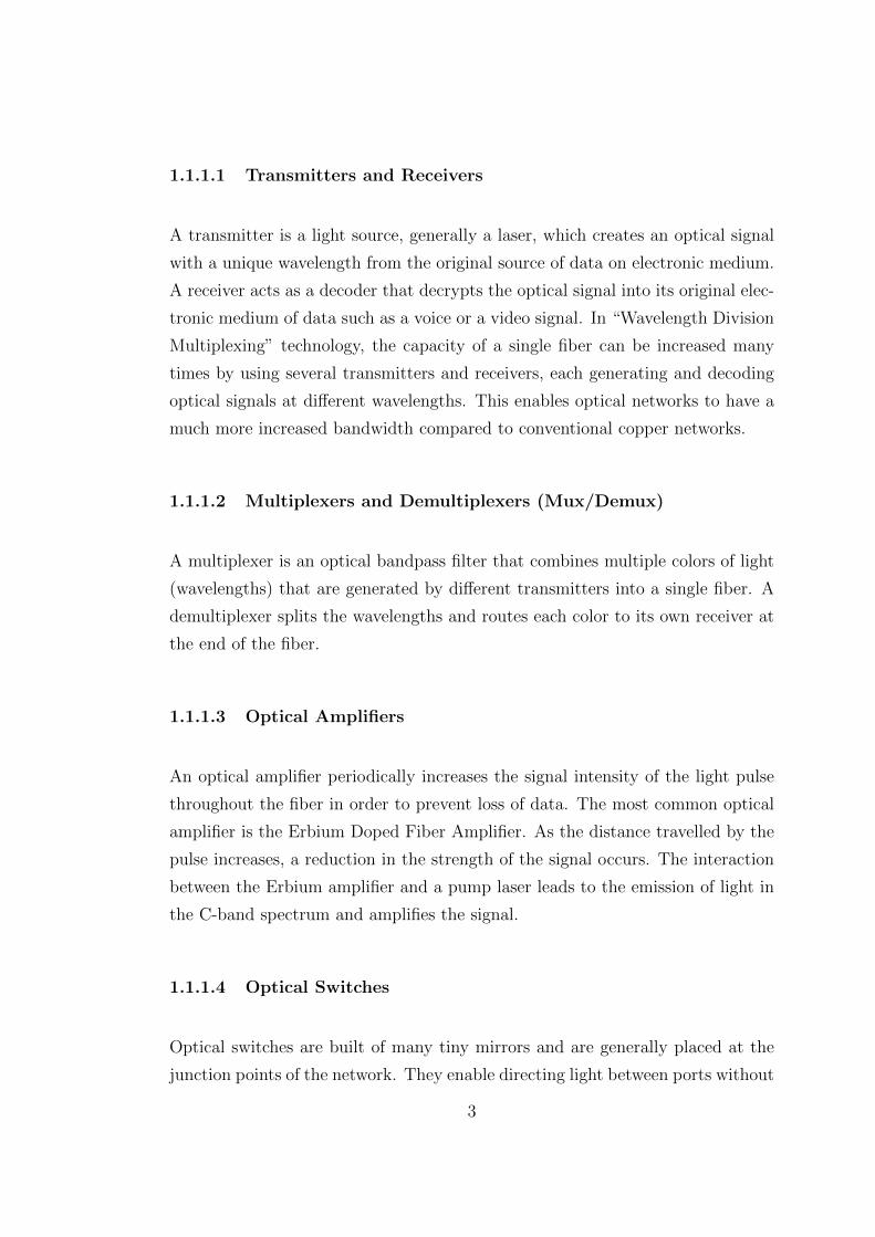
The continuous growth of demand on internet requires high speed connection and

larger capacity on telecommunication networks. In order to satisfy the day-by-day

increasing connection requests, a new modulation technique named Orthogonal

Frequency Division Multiplexing (OFDM), which promises faster connection and

better usage of optical spectrum has been developed in optical networks. In this

thesis, we propose solution methods for the Routing and Spectrum Allocation

problem that has emerged with the adaptation of OFDM technology. Our goal

is to find the minimum amount of spectrum slots that can be used while routing

connection requests from their source to destination and allocating an adequate

spectrum to the signals. We provide a new integer linear programming formula-

tion for RSA and an improved formulation for the RSA problem with a predefined

set of paths. We also propose two heuristic algorithms, Least Cost Slot Alloca-

tion and Iterative Common Path Allocation, and provide computational tests to

illustrate the performance of our ILP model and heuristic algorithms.

Keywords: Routing and Spectum Allocation, SLICE, Orthogonal Frequency Di-

vision Multiplexing, Optical Networks, Static Fiber Optic, Integer Linear Pro-

gramming.

iii

OZET

STATIK FIBER OPTIK SEBEKELERDE ROTALAMAVE SPEKTRUM YERLESTIRME

Pelin Oner

Endustri Muhendisligi, Yuksek Lisans

Tez Danısmanı: Oya Karasan

Temmuz 2016

Internet agları uzerinde artan talepler telekomunikasyon sebekelerin kapa-

sitelerinin artırılması ve hızlı baglantı saglanması ihtiyaclarını dogurmustur.

Gun gectikce artan baglantı taleplerini karsılayabilmek adına daha hızlı baglantı

saglayabilen ve optik spektrumun daha etkin kullanılmasına olanak saglayan

“Dik Frekans Bolmeli Cogullama” teknigi fiber optik sebekelerde uygulanılmaya

baslanmıstır. Bu calısmada, statik fiber optik sebekelerde rotalama ve spek-

trum yerlestirme probleminin tam sayılı lineer programlama modeli ile cozum

yolları incelenmektedir. Dogrusal amac fonksiyonu olarak rotalama ve spektrum

yerlesimi sırasında kullanılabilecek en az sayıdaki spektrum diliminin belirlenmesi

secilmistir. Bu tez icerisinde rotalama ve spektrum yerlestirme probleminin en

iyi cozumune ulasabilen yeni bir tam sayılı lineer programlama modeli ve daha

onceden belirlenmis bir rota kumesi aracılıgı ile cozume ulasabilen gelistirilmis

bir tam sayılı lineer programlama modeli onerilmistir. Lineer programlama mod-

ellerine ek olarak iki adet sezgisel algoritma gelistirilmistir. Modellerin ve sezgisel

algoritmaların performanslarının olculebilmesi icin sayısal testler yapılmıstır.

Anahtar sozcukler : Rotalama ve Spektrum Yerlestirme, Dik Frekans Bolmeli

Cogullama, Optik Sebekeler, Statik Fiber Optik, Tamsayılı Lineer Programlama.

iv

Acknowledgement

I would like to express my gratitude to Prof. Dr. Oya Karasan and Dr. Kemal

Goler for all their support and guidance throughout my graduate studies and

preparing me for my PhD journey.

I would like to thank The Scientific and Technological Research Council of

Turkey (TUBITAK) for providing financial support during my graduate studies.

But above all, I would like to thank my precious family and my friends for

supporting me through all of my choices and motivating me to overcome whatever

may lie ahead in my career.

v

Contents

1 Introduction 1

1.1 Optical Networks . . . . . . . . . . . . . . . . . . . . . . . . . . . 1

1.1.1 Components of an Optical Network . . . . . . . . . . . . . 2

1.2 Wavelength Division Multiplexing (WDM) . . . . . . . . . . . . . 4

1.3 Orthogonal Frequency Division Multiplexing (OFDM) . . . . . . . 6

1.4 Routing and Spectrum Allocation Problem . . . . . . . . . . . . . 7

2 Literature Review 10

3 Routing and Spectrum Allocation Modelling 15

3.1 Christodoulopoulos et.al’s RSA ILP formulation . . . . . . . . . . 17

3.1.1 Parameters and Variables . . . . . . . . . . . . . . . . . . 18

3.1.2 Routing and Spectrum Allocation Modelling . . . . . . . . 19

3.1.3 Analysis of Christodoulopoulos et.al’s Formulation . . . . . 20

3.2 Routing and Spectrum Allocation with Predefined Set of Paths . 27

vi

CONTENTS vii

3.3 Routing and Spectrum Allocation without Predefined Set of Paths 28

4 Heuristic Algorithms 33

4.1 Least Cost Slot Allocation (LCS) . . . . . . . . . . . . . . . . . . 33

4.2 Iterative Common Path Allocation (ICPA) . . . . . . . . . . . . . 35

5 Performance Analysis for RSA ILP without Predefined Set of

Routes 40

5.1 Results for Varying Sparsity Coefficient on Random Topologies . . 42

5.2 Results for a Real Network Topology: Deutsche Telekom Network 56

5.2.1 Performance Analysis for ILPcurrentwork and Heuristic Al-

gorithms . . . . . . . . . . . . . . . . . . . . . . . . . . . . 58

5.2.2 Performance Analysis for LCS+ILP and ICPA+ILP . . . . 60

6 Conclusion 65

A Tables 69

B Code 71

List of Figures

1.1 Principle of total internal reflection. . . . . . . . . . . . . . . . . . 2

1.2 Components of a fiber optic network. . . . . . . . . . . . . . . . . 4

1.3 Bandwidth allocation in existing fixed ITU grid versus in flexible

grid. . . . . . . . . . . . . . . . . . . . . . . . . . . . . . . . . . . 5

1.4 Comparison of frequency grid slot divisions. . . . . . . . . . . . . 6

5.1 Trend of Run Time Values for Demand Number-Node Number vs

Sparsity Combinations . . . . . . . . . . . . . . . . . . . . . . . . 45

5.2 Run Time Comparison of Different Sparsity Coefficients for Small

Networks Consisting of 8 and 14 Nodes . . . . . . . . . . . . . . . 49

5.3 Run Time Comparison of Different Sparsity Coefficients for Net-

works Consisting of 25 and 50 Nodes . . . . . . . . . . . . . . . . 50

5.4 Run Time Comparison of Different Sparsity Coefficients for Large

Networks Consisting of 100 Nodes . . . . . . . . . . . . . . . . . . 51

5.5 Effects of increasing connection requests on run time values at

various network topologies for fully connected networks . . . . . . 52

viii

LIST OF FIGURES ix


various network topologies for sparsity coefficient of 0.75 . . . . . 53


various network topologies for sparsity coefficient of 0.5 . . . . . . 54


various network topologies for sparsity coefficient of 0.25 . . . . . 55

5.9 Deutsche Telekom Network . . . . . . . . . . . . . . . . . . . . . . 56

5.10 Average run time of ILP Formulation and Heuristic Algorithms for

traffic loads of 12, 15, 20, 25 and 27 commodities. . . . . . . . . . 60

5.11 Graph of average run time with an initial solution provided:

LCS+ILP and ICPA+ILP algorithms. . . . . . . . . . . . . . . . 64

B.1 CPLEX code for Integer Linear Programming Model of Routing

and Spectrum Allocation Problem with random network topology 73

B.2 CPLEX code for Integer Linear Programming Model of Routing

and Spectrum Allocation Problem with Deutsche Telekom Network

Topology . . . . . . . . . . . . . . . . . . . . . . . . . . . . . . . . 76

List of Tables

5.1 Test Results: Run Time and Objective Function Values for

Network Topologies with Sparsity Coefficient 1 consisting of

{8, 14, 25, 50, 100} nodes and traffic load of {4, 10, 30, 50, 75, 100}Demands. Gaps reported at the objective function values denote

that the results could not be attained due to 3600 CPU seconds

time limit. . . . . . . . . . . . . . . . . . . . . . . . . . . . . . . . 43

5.2 Test Results: Run Time and Objective Function Values

for Network Topologies with Sparsity Coefficient 0.75 consist-

ing of {8, 14, 25, 50, 100} nodes and Connection Requests of

{4, 10, 30, 50, 75, 100} Demands. Gaps reported at the objective

function values denote that the results could not be attained due

to 3600 CPU seconds time limit. “(no LP file)” at the objective

function value denotes that the model file (.LP) could not be pro-

duced within 3600 CPU seconds time limit. . . . . . . . . . . . . . 44






to 3600 CPU seconds time limit. “(no LP file)” at the objective

function value denotes that the model file (.LP) could not be pro-

duced within 3600 CPU seconds time limit. . . . . . . . . . . . . . 46

x

LIST OF TABLES xi






to 3600 CPU seconds time limit. . . . . . . . . . . . . . . . . . . . 47

5.5 Test Results: Run Time and Objective Function Values for

Deutsche Telekom Network Topology with Connection Requests

of 12,15,20,25 and 27 Demands . . . . . . . . . . . . . . . . . . . 57

5.6 Comparison of average run time values for ILP Formulations and

Heuristic Algorithms for demand loads of 12, 15, 20, 25 and 27

commodities. . . . . . . . . . . . . . . . . . . . . . . . . . . . . . 59

5.7 Test results of run time values for ILP and heuristic algorithms

and decrease in run time values for heuristics+ILP combinations.

Demand loads of 12, 15, 20, 25 and 27 commodities are used for

tests. Run time value 7000+ means that the results took more than

7000 CPU seconds and were automatically killed by the system. . 62

5.8 Test results of average run time values for ILP and heuristic al-

gorithms and percentage decrease in run time values for heuris-

tics+ILP combinations. . . . . . . . . . . . . . . . . . . . . . . . . 63

A.1 Run time and objective function value results for experiments con-

ducted on DT network in [9]. Results are taken from [9] directly. . 70

Chapter 1

Introduction

1.1 Optical Networks

The continuous growth of demand on internet with addition of multimedia ser-

vices and various smart appliances as smart TVs, tablet pcs, mobile phones, cloud

systems, smart home appliances as well as increasing business activities relying

on online solutions require high speed connection and larger capacity on telecom-

munications networks. The existing available capacity of data communications

cannot meet the demand on internet and it has become clear that copper wire

connections will not be efficient enough to mitigate the communication requests of

end users. Optical communication systems consisting of bundles of optical fibers

and advanced modulation formats provide high speed transmission of data over

long distances and at higher bandwidths compared to copper cables. As a result

of less attenuation in signals and being immune to electromagnetic interference,

optical cables have replaced copper wires in telecommunication networks.

An optical cable is composed of numerous thin optical fibers bundled together.

A “Multi Mode Fiber (MMF)” has a core diameter above 10 micrometers and

allows multiple modes of light to be propagated through the fiber. A MMF has a

high power of transmission but a higher level of attenuation compared to single

1

mode fibers, which results in MMF to be used for short distance communications

with many propagation paths. A “Single Mode Fiber (SMF)” has a core diameter

between 8 to 10 micrometers which allows only one mode of light to be propagated

through the fiber. Due to fewer number of light pulses sent through the fiber,

attenuation between modes of light decreases and signal travels faster and further

on the fiber. Therefore SMFs are widely used for links longer than 1000 meters.

An optical fiber acts as a waveguide for light and is composed of three layers:

the transparent “core” surrounded by the “cladding” with a lower index of re-

fraction than the core and the “buffer coat” that protects the fiber and reduces

crosstalk between fibers. Light is kept in core by a principle called “total internal

reflection”, where a pulse of light sent within the acceptance cone of the core

travels through the fiber without leaking out. Due to total internal reflection, the

loss in signal in optical fibers is very small compared to that in copper wires.

Figure 1.1: Principle of total internal reflection.[1]

1.1.1 Components of an Optical Network

An optical network primarily includes several components consisting of optical

cables, multiplexers/de-multiplexers, optical switches and amplifiers as well as

transmitters and receivers.

2

1.1.1.1 Transmitters and Receivers

A transmitter is a light source, generally a laser, which creates an optical signal

with a unique wavelength from the original source of data on electronic medium.

A receiver acts as a decoder that decrypts the optical signal into its original elec-

tronic medium of data such as a voice or a video signal. In “Wavelength Division

Multiplexing” technology, the capacity of a single fiber can be increased many

times by using several transmitters and receivers, each generating and decoding

optical signals at different wavelengths. This enables optical networks to have a

much more increased bandwidth compared to conventional copper networks.

1.1.1.2 Multiplexers and Demultiplexers (Mux/Demux)

A multiplexer is an optical bandpass filter that combines multiple colors of light

(wavelengths) that are generated by different transmitters into a single fiber. A

demultiplexer splits the wavelengths and routes each color to its own receiver at

the end of the fiber.

1.1.1.3 Optical Amplifiers

An optical amplifier periodically increases the signal intensity of the light pulse

throughout the fiber in order to prevent loss of data. The most common optical

amplifier is the Erbium Doped Fiber Amplifier. As the distance travelled by the

pulse increases, a reduction in the strength of the signal occurs. The interaction

between the Erbium amplifier and a pump laser leads to the emission of light in

the C-band spectrum and amplifies the signal.

1.1.1.4 Optical Switches

Optical switches are built of many tiny mirrors and are generally placed at the

junction points of the network. They enable directing light between ports without

3

having to perform an optical-electronic-optical conversion.

Figure 1.2: Components of a fiber optic network.[2]

With the help of optical network components, voice, video or data signals can

be encoded into light pulses and can be transmitted across an optical fiber at

many wavelengths simultaneously. Using a technique called “Wavelength Division

Multiplexing (WDM)”, optical networks can carry data thousands of times more

than the copper-based networks.

1.2 Wavelength Division Multiplexing (WDM)

Wavelength Division Multiplexing (WDM) is a multiplexing technique that en-

ables carrying numerous optical signals of separate wavelengths on the same

strand of fiber simultaneously. WDM allows bidirectional flow of data and ex-

pands the capacity of the optical network without needing any additional fiber

strands to carry data. There are two types of WDM systems, namely“Coarse

Wavelength Division Multiplexing (CWDM)” and “Dense Wavelength Division

4

Multiplexing (DWDM)”. The difference between CWDM and DWDM is the

channel spacing they use. In Coarse WDM, transmission occurs by using 16

channels with 20 nm spacing in between wavelengths of 1270 nm and 1610 nm.

The channel spacing in CWDM spans multiple transmission windows; from O

band to L band. In Dense WDM, transmission occurs only on the C band trans-

mission window (optical spectrum range of 1530 nm to 1565 nm), but with a

denser channel spacing - typically 100 GHz for 40 channels or 50 GHz for 80

channels. DWDM allows up to 40 or 80 wavelengths with bit rates up to 100

Gb/s to be effectively carried on a single fiber, however it is likely that bit rates

greater than 100 Gb/s will not fit into this scheme. [3]

Figure 1.3: Bandwidth allocation in existing fixed ITU grid versus in flexiblegrid.[3]

Dividing the optical spectrum into fixed wavelength channels leads to some

inefficiencies in terms of network utilization efficiency. Signals with larger bit

rates than 100 Gb/s overlap with the holes at the grid boundary and therefore

cannot be supported by the fixed 50 GHz grid. Another inefficiency occurs when

the bit rate of the signal is smaller than the capacity of the channel. The whole

channel is reserved to a single signal even when the bit rate is smaller than 100

Gb/s, which results in excess channel width and waste of capacity. In order to

enable spectrum savings, a new modulation technique that will enable usage of a

flexible grid and also support higher bit rates than 100Gb/s has been developed.

5

1.3 Orthogonal Frequency Division Multiplex-

ing (OFDM)

Orthogonal Frequency Division Multiplexing (OFDM) is a digital multicarrier

modulation technique that enables the usage of sub and super wavelengths for

an elastic bandwidth allocation. OFDM uses multiple subcarrier frequencies that

can be partially overlapping instead of a single wavelength carrier in WDM. These

subcarriers, namely spectrum slots, are densely spaced together but due to the

orthogonality property, OFDM signals carried on the subcarriers do not interfere

with each other or crosstalk. The capacity of a subcarrier can differ depending

on the modulation level used (BPSK, QPSK, 8-QAM), and in [4] two possible

candidate capacity schemes are proposed as the “single slot approach” with a

slot capacity of 12.5 GHz and the “double sided half slot approach” with a slot

capacity of 6.25 GHz.

Figure 1.4: Comparison of frequency grid slot divisions. a)Current ITU-T DWDM frequency grid. b)single slot approach. c)double-sided half slotapproach.[4]

6

With the development of OFDM technology, building a spectrum efficient opti-

cal network has become possible. Based on the foundations of OFDM, Spectrum-

Sliced Elastic Optical Path Network (SLICE) is a novel elastic optical network

scheme that can satisfy the flow of demand in between source and sink nodes

by using one or multiple consecutive spectrum slots. OFDM resolves the prob-

lems encountered at WDM technology such as waste of capacity at low bit rates

or overlapping with the boundaries of the fixed grid at higher bit rates. Unlike

the “rigid” bandwidth of the conventional fixed-bandwidth optical path, an optical

path in SLICE expands and contracts” according to the traffic volume and user

request, if necessary. [5] When a traffic demand requires less than a whole single

wavelength, OFDM can efficiently distribute this sub-wavelength traffic demands

data on numerous subcarriers. When a traffic demand has a super-wavelength

requirement, for example a bit rate higher than 100 Gb/s; data can be allocated

on as much consecutive subcarriers as needed without requiring a spectral gap

or overlapping with a guard band frequency. Numerous benefits of SLICE net-

works are given in [6], [7],and [8] such as spectrum savings due to expansion and

contraction quality, energy efficient network operations, and ease of reachability

and placement issues encountered in WDM networks. OFDM based SLICE net-

works provide faster and efficient traffic allocation compared to WDM networks,

however there are also important constraints that need to be considered during

allocation of traffic on spectrum slices, which is referred to as the Routing and

Spectrum Allocation (RSA) Problem in the literature.

1.4 Routing and Spectrum Allocation Problem

The traditional Routing and Wavelength Allocation (RWA) Problem defined in

WDM networks tries to allocate an optical route and fixed wavelengths to each

traffic demand present in the network. A demand gets allocated to a full wave-

length even if its traffic size is less than 100 Gb/s, which results in inefficient

utilization of optical domain. The difference of Routing and Spectrum Allocation

problem from the Routing and Wavelength Assignment problem is that RSA tries

to route and allocate each traffic demand to as much sub-carriers as needed rather

7

than capturing unnecessary spectrum slots. Furthermore, in RWA guard-band

wavelengths are pre-determined and fixed in the spectrum domain, but in RSA

any sub-carrier can be utilized as a guard-band. The presence of non-fixed wave-

lengths and guard bands complicate the light path construction and wavelength

allocation problem, and result in a requirement for a different solution approach

than traditional solution techniques for RWA.

Although OFDM distributes the traffic on only as many sub-carriers as needed

and leaves the remaining spectrum slots in full wavelength for further occupation

by different traffic demands, the sub-carriers used for each respective traffic de-

mand need to be consecutive in order to efficiently modulate and transmit data

without loss. In other words, a single traffic can be only distributed on a con-

densed number of sub-carriers which are bundled together and which have no

spectral gap in between utilized sub-carriers. This constraint of using consecu-

tive subcarriers is referred to as the contiguity constraint. Secondly, the spectrum

slices utilized for a single traffic demand has to be constant throughout the optical

path of this traffic. In other words, each single traffic cannot change the wave-

length (or subcarriers) it is assigned to and it has to utilize the same indexed

sub-carriers throughout all of the edges/connections it passes through. This con-

straint of using the same index starting slot and utilized sub-carriers is referred

to as the continuity constraint. Thirdly, there has to be a number of guard band

spectrum slots, namely guard-carrier constraint, that separate traffic demands

which utilize common arcs in their respective optical paths, in order to provide

easier optical signal filtering.

There are two versions of RSA problem: static and dynamic. In static, or

offline RSA problem, traffic demands’ information are known prior to the planning

phase of routing and spectrum allocation, and is assumed to be steady until the

solution. Each new arriving traffic in the network requires a different routing and

solution in offline RSA problem. In dynamic, or online RSA problem, the arrival

rate and source-sink allocation of traffic demands are not known beforehand. The

scope of this thesis is limited to offline RSA problem and it intends to provide an

exact solution approach to find the routing of each traffic demand and the total

minimum number of utilized spectrum slices in the static RSA problem, taking

8

the above mentioned constraints into consideration.

To the best of our knowledge, most of the work done on Routing and Spectrum

Allocation Problem in literature takes a predefined set of paths into considera-

tion during the routing phase. However, taking a selected subset of potential

routes and limiting the search space within a preset of paths prevents the global

optimum to be found. We have encountered only in [9] an ILP formulation that

searchs the entire solution space. In this thesis, we aim to provide a different and

more efficient ILP formulation which spans all of the routes in a given network

and that can solve instances for larger graphs in lower run time values. The rest

of this thesis is organized as follows: In Chapter 2, we provide a literature review

on existing formulations for Routing and Spectrum Allocation problem. In Chap-

ter 3, we analyze the formulation of Christodoulopoulos et.al’s [10] formulation

for RSA ILP with predefined set of paths, which is a benchmark for Routing

and Spectrum Allocation problem. We propose two lemmas to strengthen their

formulation and provide a stronger ILP for RSA with predefined set of paths.

Then we define a global ILP that spans all of the solution space, namely “RSA

without Predefined Set of Paths” (also referred as ILPcurrentwork). In Chapter

4, we propose two construction heuristic algorithms for the RSA problem and

finally in Chapter 5, we provide experimental results for our ILP formulation and

heuristic algorithms.

9

Chapter 2

Literature Review

Christodoulopoulos et al, [10] address Routing and Spectrum Allocation (RSA)

problem to determine optimal allocation scheme in OFDM based Spectrum Sliced

Elastic (SLICE) Optical Path Networks. They are the first to introduce RSA

problem in replacement to the traditional Routing and Wavelength Assignment

(RWA) problem. The proposed RSA model tries to minimize the spectrum used

to serve the traffic matrix, with the assumptions that the traffic matrix (source-

destination pairs and demand sizes) is known and all demands are served, i.e. no

demand gets rejected.

There are two formulations in [10], namely (i) RSA ILP and (ii) R+SA. In the

ILP formulation, authors define an integer linear model that tries to minimize

the maximum number of spectrum slices used in any arc while allocating an

adequate spectrum scheme through selection of paths from a pre-computed set of

paths for each traffic demand. In sub-problem version of ILP, R+SA, they first

form a set P* from the pre-computed set of paths for each demand (R) and pass

this information to the second phase of spectrum allocation (SA). For heuristics,

the authors propose a Single Demand RSA Heuristic Algorithm and a Simulated

Annealing Meta-Heuristic.

The authors evaluate the performance of their proposed algorithms by using

10

computational tests in MATLAB and LINDO API. They consider two cases for

experiments: (i) A small network topology with 6 nodes and (ii) A generic network

topology with 14 nodes and 46 directed links (Deutsche Telekom Network). They

use two different values of traffic demand: D=4 as low load case and D=30 as

high load case. The distribution of the demand width value, Tsd for connection

(s,d), is chosen as uniformly distributed between 0 and D. Results show that for

small network topology, RSA model finds a solution in an average of 3.25 seconds

for low load case and 503.19 seconds for high load case. R+SA formulation finds a

solution faster; 2.72 seconds for low load, 6.48 seconds for high load. For realistic

network topology, RSA was not able to produce results and R+SA finds the best

solutions within 2 hours. The shortcoming of both of these formulations is that

a global minimum is not guaranteed as the algorithm does not cover all paths,

but uses a set of pre-computed paths.

Further on, Christodoulopoulos, Tomkos and Varvarigos [11] address an exten-

sion of the RSA problem by adding modulation level constraint. They introduce

Routing, Modulation Level, and Spectrum Allocation (RMLSA) problem which

tries to minimize the spectrum used to serve the traffic matrix via choosing an

appropriate modulation level with respect to the transmission distance. They

break the problem into two sequential sub-problems: namely (i) Routing and

Modulation Level (RML) and (ii) Spectrum Allocation (SA). Further on, they

propose a sequential heuristic algorithm that serves all the connections in the

traffic matrix one by one by using simulated annealing meta-heuristic to obtain

orderings.

The authors evaluate the performance of their proposed algorithms by using

computational tests in MATLAB and LINDO API. For all algorithms they use

3 pre-computed paths for each demand and two load cases (D=4 for low load

traffic and D=30 for high load traffic). They use two network topologies; one

consisting of a 6 node small network and another a 14 node generic Deutsche

Telekom topology. Computational results show that for the small network topol-

ogy, RMLSA produces a solution in average 3.25 seconds for low load and 503.19

seconds for high load traffic cases. RML+SA produces a solution in average 2.72

seconds for low load and 6.48 seconds for high load traffic cases. For DT network,

11

RMLSA could not produce results and RML+SA could produce solutions only

after 2 hours.

Wang et al, [12] prove NP-hardness of the static RSA problem and present a

different RSA ILP formulation to optimally allocate the sub-carriers (slices) and

guard-carriers in SLICE networks in their work. They analyze the upper/lower

bounds of the number of slices needed in different topologies and present two

heuristic algorithms; (i) Balanced Load Spectrum Allocation (BLSA) and (ii)

Shortest Path with maximum Spectrum Reuse (SPSR). Like Christodoulopoulos

et al, they try to minimize the maximum number of subcarriers required in any

fiber of a SLICE network. They test the upper/lower bounds of their formulation

in two cases of Ring Network topology with and without predetermined routing.

The authors evaluate the performance of their algorithms by using computa-

tional tests in ILOG CPLEX. They have found out that the lower bound for the

ILP model on Ring Networks can be achieved by the cut-set (CS) method. They

test their ILP model on two Ring networks with 4 and 5 nodes and uniform traffic

demand. For the heuristics proposed, they use two different network topologies

to compare the performance of the algorithms with the ILP model; 6 nodes for

a small network and 14 nodes for a large network. The computational results of

their simulations show that for uniform network demands, heuristic algorithms

produce close solutions to the optimal ILP model. However, there is no infor-

mation on the computation times to find the optimal solution for the ILP model

and/or heuristics.

Velasco et al, [13] approach to the problem of routing and spectrum allocation

by eliminating the complexity that the contiguity constraint gives by defining a

concept of channels for the representation of contiguous spectral resources. They

introduce Channel Assignment (CA) as an equivalent of Wavelength Assignment

(WA) approach in WDM, which tries to minimize the number of rejected demands

based on the assignment of demands on channels using a pre-computed set of

channels as input. The authors propose two ILP formulations for the CA problem:

(i) a link-path formulation and (ii) a node-link formulation. They also formulate a

relaxed version of the RSA problem which does not consider spectrum continuity

12

constraint, in order to obtain lower bounds.

The authors evaluate the performance of their algorithms by using 5 different

network topologies; Ring9 (9 nodes, 9 edges), Brasil network (10 nodes, 12 edges),

Abilene network (12 nodes, 15 edges), Spanish Telefonica (21 nodes, 35 links) and

Deutsche Telekom network (14 nodes, 23 edges). They create 36 demands with

a uniform distribution between 1 and 4 slices. CA model finds a solution in over

6 hours both for the link-path approach and the node-link approach.

Klinkowski and Walkowiak [14], formulate the RSA problem with an objec-

tive of minimizing the number of frequency slots that are assigned to at least

one demand in the network. Similar to [10], they use a set of predefined paths

to solve the problem. They also propose a novel heuristic Adaptive Frequency

Assignment-Collision Avoidance, namely AFA-CA, which estimates the number

of frequency slots that might be allocated to a link taking all candidate paths

into account and then adaptively selects demands to be assigned on the spectrum

such that the less congested path and lowest indexed frequency slots are picked for

each demand. They test their ILP formulation on a small 6 node 16 links network

with different combinations of frequency slot requirement distribution-demand

number pairs and AFA-CA algorithm on a small 6 node 16 links, NSFNET(15

node 46 links) and UBN24 (24 node 86 links) networks. Results show that the

ILP formulation has a run time value ranging from 13 seconds for a demand

number of 30 demands with frequency slot requirements of Uniform(0,5) and to

12747 seconds for a demand number of 15 with frequency slot requirements of

Uniform(0,30). The experiment shows that as the number of frequency slot re-

quirements increases, ILP formulation of [14] produces longer run time values.

For their proposed heuristic AFA-CA, the results show that the heuristic has a

run time value of about 1 seconds and has an optimality gap ranging from 2.49%

to 7.02%. The authors state that the main difficulty for their ILP formulation

comes from the huge number of constraints which occurs when large number of

frequency slots are required by a demand in some network scenarios. No further

analysis on run time values in larger networks are present in [14].

Paul [9] proposes an ILP model to optimally solve the RSA problem with the

13

objective of finding the minimum number of spectrum slots used while allocating

demand in OFDM based optical networks. The first formulation, namely ILP1,

spans all network and tries to allocate all demands by finding the optimal routing

scheme and spectrum allocation. The second formulation proposed by the author,

namely ILP2, takes a pre-determined routing scheme for the demands and allo-

cates spectrum slots according to these schemes. The author then compares his

formulations with Christodoulopoulos et al’s ILP formulation (CHR) and con-

ducts performance analyses. Performance analyses are conducted using ILOG

CPLEX and consist of 8, 12, 15, 18 and 20 commodities and 3 pre-computed

paths for each commodity. Topologies of 8, 12, 15 node networks and 14 node

Deutsche Telekom network are used. The results of [9]’s experiments show that

ILP1 formulation can process up to 15 demands in 15 node networks, with an

average run time value of 824,31 seconds. In real-life network topology, the au-

thor uses Deutsche Telekom(14 nodes, 23 edges) network and the results for ILP1

show that the formulation can handle up to 20 demands with an average run time

value of 896,02 seconds.

In this thesis, we propose a different and more efficient ILP formulation that

spans all possible routes and finds a global optimum to the RSA problem. The

performance analysis of our proposed ILP formulation, ILPcurrentwork, show that

our formulation can solve instances for up to 50 demands in 8,14 and 50 node

networks, up to 100 demands in 25 node networks and up to 30 demands in

100 node networks for complete graphs. For real-life network topology, we use

Deutsche Telekom(14 nodes, 23 edges) network similar to [10] and [9], and our for-

mulation can handle up to 25 demands with an average run time value of 646,58

seconds. The complete test results for varying sparsity, total demand numbers

and number of nodes in the graph can be seen in Chapter 5. When compared to

Christodoulopoulos et.al [10], Klinkowski and Walkowiak [14] and Paul [9] exper-

iments, the results of our experiments show that our ILPcurrentwork formulation

can solve instances for larger graphs, for larger frequency slot distributions (we

have taken frequency slot distributions from Uniform(0,50)) and has lower run

time values.

14

Chapter 3

Routing and Spectrum

Allocation Modelling

In this chapter, we analyze the ILP formulation for Routing and Spectrum Allo-

cation in [10] that acts as a benchmark for RSA problem and define two lemmas

to strengthen the model. Then from our proposed formulation, we derive an-

other ILP model that considers every path during routing and allocation phase

and provides a global solution to the RSA problem. To the best of our knowledge,

such a global formulation is only proposed by [9] in the literature, and we aim to

provide a more efficient formulation that can solve instances for larger networks.

In the static RSA problem, a connection request, i.e. a demand d, which

originates from a source node u(d) has to be transferred to its destination, the

sink node v(d), by traversing an optical route that connects u(d) to v(d). In order

to be sent as a light pulse from its source node to sink node, each demand has

to be assigned to a number of frequency slots (or spectrum slots) in the optical

spectrum such that there is no crosstalk between demands that share an edge in

their optical routes. Each demand has a bandwidth which denotes the length of

the signal and is translated into the size of the demand as a number of spectrum

slots by dividing the bandwidth of the demand to the capacity of each subcarrier,

assuming that the capacity of each subcarrier is constant and fixed. In order to

15

formulate the RSA problem as an ILP, we assume that we have a graph consisting

of the hubs in the network and we assume that the graph is connected. We assume

that the nodes in the graph represent the hubs in the network and the edges that

connect nodes represent physical fiber optic cables. As fiber optic cables can carry

bidirectional information, a single link of cable represents an edge in the graph.

We assume that the total connection requests form the demand set D, and the

information of all demands in the set D are known prior to the planning phase of

the RSA problem. Within the context of this assumptions, the objective of the

static RSA problem is to find the minimum number of spectrum slots required

to route and assign spectrum slots to each demand in the demand set D. We

assume that no demand gets rejected, i.e. all of the demands are allocated to a

route and adequate spectrum slots.

In order to find the number of spectrum slots in the visible light spectrum,

we use the formula λ = cF

where λ is the wavelength, c is the speed of the light

and F is the frequency. Taking the visible light’s spectrum as 400nm to 700nm,

taking λ1 = 400nm and λ2 = 700nm and solving for corresponding F ’s result

that the frequency of the visible light is between 430 THz and 750 THz, which

is an approximately 320000 GHz interval. Taking each spectrum slot with a 12.5

GHz capacity results that the visible spectrum has 32000012.5

= 25600 slots. As to

completely occupy 25600 slots in the spectrum require much more amount of

traffic requests with huge demand sizes than the RSA problem can be solved for,

we assume that the edges are uncapacitated.

The important constraints to be considered in Routing and Spectrum Alloca-

tion problem are continuity, contiguity, guard-carrier and non-overlapping spec-

trum constraints. Continuity constraint requires that each demand has a steady

spectrum slot allocation throughout its path, i.e. has the same starting slot al-

location at each of the edges it uses in its path. Contiguity constraint requires

that each demand is allocated on spectrum slots that are bundled together and

have no spectral gaps in between. Non-overlapping spectrum constraint requires

that for demands sharing an edge, a spectrum slot can only be allocated to a

single demand in order to prevent crosstalk (the direction of the demands are not

important as an edge can carry bidirectional information and crosstalk can occur

16

without depending on the direction). Guard-carrier constraint requires that for

demands sharing an edge, the spectrum allocation of these demands have to be

separated by a number of slots, referred to as the guard carrier.

3.1 Christodoulopoulos et.al’s RSA ILP formu-

lation

The joint formulation of Christodoulopoulos, Tomkos and Varvarigos [10] con-

siders demand allocation in OFDM based Optical Spectrum SLICE Network with

pre-computed paths. The Integer Linear Programming (ILP) formulation con-

siders an offline network with a given traffic matrix consisting of source, demand

and requested transmission rates; and tries to minimize the utilized spectrum

while serving the connections through adequate spectrum allocation, with the

constraint that no spectrum overlapping is allowed and each traffic demand is

assigned consecutive spectrum slots (contiguity).

The assumptions of the formulation are as follows:

1. The spectral granularity of the transmitters and WXCs is one subcarrier

corresponding to F GHz of spectrum.

2. The capacity of a subcarrier is equal to C Gbps and is taken as constant

without taking the modulation level into consideration.

3. A guardband of G subcarriers seperates adjacent spectrum paths.

4. Serving a connection i that requires Ti subcarriers is translated to finding a

starting subcarrier frequency fi after which it can use Ti contiguous subcarriers.

5. Assuming a constant subcarrier capacity C, a bandwidth demand of Bi can

be mapped to a demand of Ti subcarriers as Ti = dBi

Ce.

17

3.1.1 Parameters and Variables

The network topology of the RSA problem is denoted by a connected graph

G =(V ,E), where V is the set of nodes and E is the set of edges (i.e. fiber

links) connecting the nodes. Given the graph G and the demand set D, the aim

of this formulation is to choose a route from the source node to the destination

node for each demand, from the pre-determined route set Pd, and an allocation

in the optical spectrum (i.e. indices of frequency slots) that is constant in all

edges the demand traverses in its chosen path. A demand d = (u(d), v(d)) is

a connection request which originates from node u(d) and terminates at node

v(d). In the static RSA problem, the demands’ information –source node, sink

node and demand size– is known prior to the planning phase. T (d) denotes the

number of subcarriers required (i.e. the demand size) for the communication d

between source u(d) and destination v(d); such that T (d) ≥ 0,∀d ∈ D. For each

commodity d ∈ D, k paths are pre-calculated, i.e. |P (d)| = k.

Sets and Parameters:

Pd: The set of k candidate paths for connection d.

P=∪dPd: The total set of candidate paths for the demand set D.

G : The amount of subcarriers required as guardband in between demands that

use the same edge in their paths, and is taken as constant.

T (d): The number of subcarriers required for the communication between

source u and destination v.

Variables:

Xp: 0 if path p is not utilized , and 1 if p is utilized.

S(d): Integer variable that denotes the starting frequency for connection d =

(u(d), v(d)). Assuming Ttotal =∑

d T(d), 0≤ S(d)≤ Ttotal.

18

Wdk,dt : Boolean variable that equals 1 if the starting frequency of connection

dk is smaller than the starting frequency of connection dt (i.e. Sdk < Sdt) and 0

otherwise.

c: Maximum utilized spectrum slot number.

3.1.2 Routing and Spectrum Allocation Modelling

minimize c (3.1)

subject to : ∑p∈Pd

Xp = 1 ∀d ∈ D (3.2)

c ≥ S(d) + T (d) ∀d ∈ D (3.3)

If ∃p ∈ Pdk and ∃q ∈ Pdt such that p∩ q 6= ∅, then for each dt , dk ∈ D and every

p, q ∈ P the following equations (3.4-3.8) are employed:

Wdk,dt +Wdt,dk = 1 (3.4)

S(dk)− S(dt) ≤ Ttotal ∗Wdt,dk (3.5)

S(dt)− S(dk) ≤ Ttotal ∗Wdk,dt (3.6)

S(dt) + T (dt) +G− S(dk) ≤ (Ttotal +G) ∗ [1−Wdt,dk + 2−Xp −Xq] (3.7)

S(dk) + T (dk) +G− S(dt) ≤ (Ttotal +G) ∗ [1−Wdk,dt + 2−Xp −Xq] (3.8)

Xp ∈ {0, 1} p ∈ P (3.9)

S(d) ≥ 0 d ∈ D (3.10)

Wdt,dk ∈ {0, 1} dt, dk ∈ D (3.11)

19

3.1.3 Analysis of Christodoulopoulos et.al’s Formulation

Number of variables and constraints

There are |P| binary X variables, |D| continuous S variables and |D|∗|D−1|2

binary W variables. In total there are |P| + |D|+ |D|∗|D−1|2

variables in the for-

mulation.

For each value of d, there is one constraint for (3.2) and in total, the number

of constraints for (3.2) are |D|. In the same manner, there are |D| constraints for

(3.3). For constraints (3.4), (3.5) and (3.6) there are |D|∗|D−1|2

constraints for each

of the respective equations. For constraints (3.7) and (3.8) there are |Pdk | ∗ |Pdt |constraints for each demand pair dk,dt. As each demand has k precalculated

paths, i.e. as |Pd| = k; ∀d ∈ D, there are k2 ∗ |D|∗|D−1|2

constraints in total for

each equation. Therefore, the total number of constraints in the formulation are

2 ∗ |D|+ 32∗ |D| ∗ |D − 1|+ k2 ∗ |D| ∗ |D − 1|.

The overall complexity for variables are O(|D|2 + |P|) and O(|D|2 ∗ k2) for

constraints.

20

Analysis of the constraints

Given a set of pre-computed paths for each connection request d, equation (3.2)

ensures that only one of these paths would be chosen for each of the connection

requests. Equation (3.3) computes the maximum index of spectrum slot that each

connection terminates at. Together with the equation (3.3), objective function

minimizes the maximum number of spectrum slots used.

Maintaining a single starting slot index throughout all links that each demand

uses, S(d): ∀d ∈ D, satisfies the continuity constraint of the RSA problem.

In order to satisfy the contiguity and non-overlapping spectrum constraints, the

demands that share at least one common link in their respective paths have to be

allocated on the spectrum such that each spectrum slice is allocated to at most

one demand. In order to ensure this, equations (3.4)-(3.8) are employed for all

demands that share at least one common arc in their respective paths: dt, dk ∈ Dsuch that ∃p ∈ Pdk and ∃q ∈ Pdt where p ∩ q 6= ∅. Equations (3.4)-(3.6) ensure

that for every demand pair that shares a common fiber arc in their paths, one of

these demands should be placed before the other in the optical spectrum. Note

that if either one (or both) of Xp and Xq is 0, this means that the overlapping of

these demands on these paths is not important, therefore sorting of the demands

is not necessary. Therefore, we have to look at the case where both Xp and Xq

are 1. Assuming that dt and dk share at least one arc in their paths, lets place

demand dt in front of demand dk, which means that Wdt,dk = 1, to analyze these

constraints.

Taking Wdt,dk = 1 ensures that Wdk,dt = 0 in our case by equation (3.4). As

Wdt,dk is 1 and Wdk,dt is 0, constraint (3.6) ensures that the starting frequency slot

of demand dt is smaller than demand dk, which means that dt is placed before dk.

Constraint (3.5) is deactivated when Wdt,dk is 1; S(dk)−S(dt) ≤ Ttotal is trivially

satisfied as we have S(d) ≤ Ttotal ∀d ∈ D.

Contiguity constraint is satisfied by equations (3.7) and (3.8). Constraint (3.7)

becomes:

S(dt) + T (dt) +G− S(dk) ≤ (Ttotal +G) ∗ [1− 1 + 2− 1− 1]

21

since bothXp andXq are 1 as they utilize paths p and q; andWdt,dk is 1. Therefore

the right hand side of the equation is 0, yielding in

S(dt) + T (dt) +G ≤ S(dk)

This constraint ensures that demand dk is placed at least a number of the demand

size of dt plus a guardband slices after demand dt.

Similarly, Constraint (3.8) becomes:

S(dk) + T (dk) +G− S(dt) ≤ (Ttotal +G)

which is reduced to

S(dk) + T (dk) ≤ S(dt) + Ttotal

Likewise constraint (3.5), this constraint also ensures that the demand dk stays

within the boundaries of the total sum of the demand sizes.

Lemma 1: Equations (3.5) and (3.6) are implied by equations (3.7) and (3.8)

and can be eliminated from the model.

Proof: Recall - Equation (3.7)

S(dt) + T (dt) +G− S(dk) ≤ (Ttotal +G) ∗ [1−Wdt,dk + 2−Xp −Xq]

For Wdt,dk = 1 and Xp = 1 and Xq = 1, equation (3.7) becomes

S(dt) + T (dt) +G− S(dk) ≤ (Ttotal +G) ∗ [1− 1 + 2− 1− 1]

S(dt) + T (dt) +G− S(dk) ≤ (Ttotal +G) ∗ [0]

S(dt) + T (dt) +G− S(dk) ≤ 0

S(dt) + T (dt) +G ≤ S(dk)

S(dk) ≥ S(dt) + T (dt) +G

As Tdt ≥ 0 and G ≥ 0, the above equation implies that;

S(dk) ≥ S(dt) (3.12)

22

Recall - Equation (3.6):

S(dt)− S(dk) ≤ Ttotal ∗Wdk,dt

As we already know that Wdk,dt = 0 holds when Wdt,dk = 1 by equation (3.4),

equation (3.6) becomes;

S(dt)− S(dk) ≤ Ttotal ∗ 0

S(dt)− S(dk) ≤ 0

S(dt) ≤ S(dk)

S(dk) ≥ S(dt)

As the above inequality is already suggested by equation (3.7) via (3.12), equation

(3.6) can be eliminated from the model.

Likewise, for equations (3.8) and (3.5), we can apply the same steps.


S(dk) + T (dk) +G− S(dt) ≤ (Ttotal +G) ∗ [1−Wdk,dt + 2−Xp −Xq]

For Wdk,dt = 0 and Xp = 1 and Xq = 1, equation (3.8) becomes

S(dk) + T (dk) +G− S(dt) ≤ (Ttotal +G) ∗ [1− 0 + 2− 1− 1]

S(dk) + T (dk) +G− S(dt) ≤ (Ttotal +G) ∗ [1]


S(dk) ≤ S(dt) + Ttotal − T (dk)

As T (d) ≥ 0 ∀d ∈ D; Ttotal =∑

d T(d) ≥ 0 and Ttotal ≥ T (dk) ≥ 0, ∀(dk) ∈ D.

Therefore the following always holds: Ttotal−T (dk) ≥ 0 and Ttotal−T (dk) ≤ Ttotal.

Hence S(dt) + Ttotal − T (dk) ≤ S(dt) + Ttotal and this implies that

S(dk) ≤ S(dt) + Ttotal − T (dk) ≤ S(dt) + Ttotal

S(dk) ≤ S(dt) + Ttotal (3.13)

23


S(dk)− S(dt) ≤ Ttotal ∗W (dt)(dk)

As we already know that W (dt)(dk) = 1, equation (3.5) becomes;

S(dk)− S(dt) ≤ Ttotal ∗ (1)

S(dk)− S(dt) ≤ Ttotal

S(dk) ≤ S(dt) + Ttotal

As the above inequality is already suggested by equation (3.8) via (3.13), equation

(3.5) can be eliminated from the model.

The same steps apply if we take Wdk,dt = 1 and Wdt,dk = 0, but in that case

equation (3.7) will imply equation (3.5); and (3.6) will be deactivated and also

be implied by (3.8).

Taking a multiplier of (Ttotal + G) in equations (3.4) and (3.5) creates an

upperbound for the number of spectrum slots to be used when there are at most

2 demands that share a common link in their paths; however this bound is not

enough for congested cases when there are 3 or more demands that share a link

in their paths as it diminishes the total amount of guardband required in between

demands.

Lemma 2: The multiplier on the right hand side of equations (3.7) and (3.8)

must be an upperbound for the slots of the last demand assigned on a link; and

should be replaced by[Ttotal +

∑|D|d=1G

], where Ttotal =

∑d∈D T (d).

Proof:

Assume that there are n demands D = {dti : i = 1...n} that all share a common

link in their paths (∃pi ∈ Pdti∀i ∈ {1...n} such that p1 ∩ p2 ∩ ... ∩ pn 6= ∅).

Taking the most congested case into consideration (i.e. when there is exactly

one arc, say (j, k), present in the graph and all dti , i ∈ {1...n} have exactly one

path Pi that uses (j, k)), we have to make sure that all demands can be allocated

to as many spectrum slots as needed. As all demands use arc (j, k), we have

24

XPi= 1 ∀i ∈ {1...n}. Take any two demands dt, dk from the demand set D and

let Wdt,dk = 1, meaning demand dt is placed before dk.

From equation (3.4), we have Wdk,dt = 0. Equation (3.7) becomes

S(dt) + T (dt) +G− S(dk) ≤ 0

S(dk) ≥ S(dt) + T (dt) +G (3.14)

and Equation (3.8) becomes


S(dk) + T (dk) +G ≤ S(dt) + (Ttotal +G) (3.15)

For any demand dk ∈ D, we have (n − 1) constraint pairs of (3.14) and (3.15).

Equation (3.14) assigns the starting slot index of dk, S(dk), as greater than the

size of demand dt+ guardband; and demand dk is placed at the end of all present

demands on the common arc by taking the largest S(dk) value among all Equa-

tions (3.14) for demand dk. Note that the same applies to all demands that are

placed before dk.

From equation (3.15), demand dk has to be assigned such that the endpoint of dk

is within the boundary of S(dt) + Ttotal. The lower bound of all right hand side

values of (3.15) occurs at S(d0) + Ttotal, where S(d0) denotes the starting slot of

the first assigned demand (which is the minimum among all S(di)’s). Note that

the right hand side value of this constraint applies to all demands in the same

way, since S(d0) +Ttotal ≤ S(di) +Ttotal as we know S(d0) ≤ S(di) ∀i ∈ D. Hence

we can say that S(di) + T (di) + G ≤ S(d0) + (Ttotal + G) is the constraint that

defines the upperbound for all S(di) values.

Let the multiplier of equations (3.7) and (3.8) be X and let X=Ttotal + G.

Regardless of the sorting of the demands, this occurs as an upperbound for all

S(di) and becomes problematic for the last demand assigned. In order to make

sure that the last demand is still in the spectrum, we have to analyze whether

X=Ttotal + G is an adequate upperbound. Let dk be the last demand to be

assigned on the spectrum. We have (n− 1) constraint couples of

S(dk) ≥ S(dt) + T (dt) +G

25

S(dk) + T (dk) +G ≤ S(dt) + X

for t ∈ D/{k}. The largest of the first constraint’s right hand side occurs at the

last demand before k, say t, and the lowest of the right hand side of the second

equation occurs at S(d0) + X − T (dk) − G (when S(dk) is left alone on the left

hand side). In order for S(dk) to have a value, we have to satisfy

S(dt) + T (dt) +G = S(d0) + X − T (dk)−G (3.16)

Solving for X results

X = S(dt) + T (dt) + T (dk)− S(d0) + 2G (3.17)

We know that dt is the demand right before dk. For dt we have constraints

S(dt) ≥ S(d′t) + T (d′t) +G

and

S(dt) + T (dt) +G ≤ S(d0) + X

where d′t is the last demand before dt. In order for any demand t to be assigned,

equation (3.16) must be satisfied. Hence whenever dt has a solution, we have

S(dt) = S(d′t) + T (d′t) + G. When we substitute S(dt) into equation (3.17), we

get

X = S(d′t) + T (d′t) +G+ T (dt) + T (dk)− S(d0) + 2G

In a similar fashion when we solve for all S(d′t) iteratively, we get the equation

X = [S(d0)+T (d0)+...+T (d′′t )+(n−3)∗G]+T (d′t)+G+T (dt)+T (dk)−S(d0)+2G

which reduces to

X = S(d0) +n∑

i=1

T (di) +n∑

i=1

G− S(d0)

and finally

X =n∑

i=1

T (di) +n∑

i=1

G (3.18)

As we can see, X = Ttotal +G does not appear as an adequate upperbound, and

has to be updated as∑

d∈D T (d) +∑|D|

i=1G.

26

3.2 Routing and Spectrum Allocation with Pre-

defined Set of Paths

As we have found out in the previous section, equations (3.5) and (3.6) can

be eliminated from Christodoulopoulos et al’s formulation of RSA ILP, and the

upperbound for equations (3.7) and (3.8) should be updated as X =∑|D|

i=1 T (di)+∑|D|i=1G. Within the context of the same assumptions, the new formulation will

have |D|∗ |D−1| constraints less than the latter and hence will be faster in terms

of computational time.

Hence, the new model for the RSA within the context of same assumptions can

be formulated as the following:


Pd: The set of k candidate paths for connection d.

P=∪dPd: The total set of candidate paths for the demand set D, d ∈ D.



T (d): The number of subcarriers required for the communication d between

source u(d) and destination v(d).

Variables:

Xp: 0 if path p is not utilized , and 1 if p is utilized;

S(d): Integer variable that denotes the starting frequency for connection d;

Wdk,dt : Boolean variable that equals 1 if the starting frequency of connection dk

is smaller than the starting frequency of connection dt (i.e. Sdk < Sdt) and 0

otherwise;

27


minimize c (3.19)

subject to : ∑p∈Pd

Xp = 1 ∀d ∈ D (3.20)

c ≥ S(d) + T (d) ∀d ∈ D (3.21)

If ∃p ∈ Pdk and ∃q ∈ Pdt such that p∩ q 6= ∅, then for each dt , dk ∈ D and every

p, q ∈ P equations (3.22-3.24) are employed:

Wdk,dt +Wdt,dk = 1 (3.22)

S(dt) + T (dt) +G− S(dk) ≤ X ∗ [1−Wdt,dk + 2−Xp −Xq] (3.23)

S(dk) + T (dk) +G− S(dt) ≤ X ∗ [1−Wdk,dt + 2−Xp −Xq] (3.24)

Xp ∈ {0, 1} p ∈ P (3.25)

S(d) ≥ 0 d ∈ D (3.26)

Wdt,dk ∈ {0, 1} dt, dk ∈ D (3.27)

where Ttotal =∑

d∈D T (d) and X =∑

d∈D T (d) +∑|D|

i=1G;

3.3 Routing and Spectrum Allocation without

Predefined Set of Paths

In the previous section, we have found an improved model for the offline routing

and spectrum allocation problem with a set of predetermined routing for each

demand. Although [10] have shown that their version of RSA problem can reach

to near optimal solutions, this model does not guarantee a global optimum as it

excludes many feasible paths that can generate optimal solutions. A new model

that spans every feasible path to find the global optimum for routing and spectrum

28

slot selection within the context of the same assumptions as the previous sections

can be formulated as follows:

We assume that we are given a connected graph G =(V ,E),where V is the

set of nodes and E is the set of edges, a bandwidth demand of d corresponds

to a connection request with source u(d) and sink v(d) and D is the set of all

connection requests. The aim of this formulation is to provide a route from the

source node u(d) to the destination node v(d) of each demand and an allocation in

the optical spectrum (i.e. indices of frequency slots) that is constant in all edges

the demand traverses in its path. In this formulation, no pre-calculated routes

are present. A route for each demand is determined by flow balance equations in

the formulation.


D: Set of connection requests, i.e. demands.

A={(i, j) ∪ (j, i) : {i, j} ∈ E}: The arc set generated from the edge set E of

graph G.



T (d): The number of subcarriers required for the communication d between source

u(d) and destination v(d).

Variables:

Xijd: boolean arc utilization variable that equals 0 if demand d does not use arc

(i, j); and 1 if d uses arc (i, j).

S(d): Integer variable that denotes the starting frequency for connection d.

Wdk,dt : Boolean variable that equals 1 if the starting frequency of connection dk

is smaller than the starting frequency of connection dt (i.e. Sdk < Sdt) and 0

otherwise.

29


Model

minimize c (3.28)

subject to :∑j:(i,j)∈A

Xijd −∑

j:(j,i)∈A

Xjid = 1 ∀d ∈ D : i=u(d) (3.29)

∑j:(i,j)∈A

Xijd −∑

j:(j,i)∈A

Xjid = 0 ∀d ∈ D : i 6= u(d), i 6= v(d) (3.30)

∑j:(i,j)∈A

Xijd −∑

j:(j,i)∈A

Xjid = −1 ∀d ∈ D : i=v(d) (3.31)

c ≥ S(d) + T (d) ∀d ∈ D (3.32)

Wdk,dt +Wdt,dk ≤ 1 ∀dk, dt ∈ D :dk 6= dt (3.33)

Wdk,dt +Wdt,dk ≥ [(Xijdt +Xjidt) + (Xijdk +Xjidk)− 1]

∀(i, j), (j, i) ∈ A ∀dk, dt ∈ D : dt 6= dk(3.34)

S(dt) + T (dt) +G ≤ S(dk) + X ∗ [1−Wdt,dk ]

∀dk, dt ∈ D : dt 6= dk(3.35)

S(dk) + T (dk) +G ≤ S(dt) + X ∗ [1−Wdk,dt ]

∀dk, dt ∈ D :dt 6= dk(3.36)

Xijd ∈ {0, 1} ∀(i, j) ∈ A, ∀d ∈ D (3.37)

S(d) ≥ 0 ∀d ∈ D (3.38)

Wdt,dk ∈ {0, 1} ∀dt, dk ∈ D (3.39)

where Ttotal =∑

d∈D T (d) and X =∑

d∈D T (d) +∑|D|

i=1G.

Analysis of RSA without Pre-Defined Set of Paths

Equations (3.29)-(3.31) are flow balance equations which ensure that each

demand will have exactly one path. Equation (3.32) along with the objective

function (3.28) is used to find the minimum of the maximum number of spec-

trum slots used among all demands. Equations (3.33)-(3.34) are used to sort

30

the demands: Equation (3.34) ensures that for demands sharing an edge {i, j},Wdk,dt +Wdt,dk ≥ 1 (as Xijdt +Xjidt = 1 and Xijdk +Xjidk = 1, and it is trivially

≥ 0 if no two demands share this arc. Equation (3.33) sets an upperbound; if two

demands do not share an edge, Equation (3.33) results in either ≥ 0 if either one

of the demands uses edge {i, j} and the other one does not; or ≥ −1 if none of

the demands uses edge {i, j}– in which case sorting of these demands is not nec-

essary. If two demands share an edge, Equation (3.33) combined with Equation

(3.34) results in Wdk,dt +Wdt,dk = 1 exactly, and force the demands to be sorted.

Equations (3.35)-(3.36) are contiguity constraints that are used for defining

the starting slot index for each demand. For demands that do not share an edge

(i.e. both Wdk,dt = 0 and Wdt,dk = 0), starting slot indices can be any value

within the boundaries. For demands that share an edge, as Equations (3.33) and

(3.34) ensure that only one of Wdk,dt and Wdt,dk will be 1, the demand that is

sorted second in the spectrum will be assigned a spectrum slot index greater than

the sum of the index of the first demand and its size plus the number of guardian

frequencies. Continuity requirement of RSA problem is satisfied by allocating

only one starting slot index S(d) for each demand and maintaining it throughout

the path.

Number of Variables and Complexity

There are |A|∗ |D| binary X variables, |D| continuous S variables and |D|∗|D−1|2

binary W variables. In total there are |D| ∗ [|A| + 1+ |D−1|2

] variables in the

formulation.

For each value of d, there is one constraint for (3.29) and for (3.31) and there

are |V | − 2 constraints for (3.30). In total, the number of constraints for (3.29)-

(3.31) are |D| ∗ |V |. In the same manner, there are |D| constraints for (3.32).

For (3.33) there are |D|∗|D−1|2

constraints. For (3.34) one edge is considered at

each equation for each demand pair and in total |E| edges are considered for each

demand. In general there are |E| ∗ |D|∗|D−1|2

constraints for (3.34). For (3.35) and

(3.36) there are |D|∗|D−1|2

constraints. Therefore, the total number of constraints

in the formulation are |D| ∗ [|V |+ 1 + |D|−12∗ [3 + |E|]].

31

The overall complexity for constraints are O(|D|2∗|E|+|D|∗|V |) and O(|D|2+

|D| ∗ |A|) for variables.

32

Chapter 4

Heuristic Algorithms

In the previous chapter, we have formulated a mathematical model that spans

all of the feasible region and yields in a global optimum solution for Routing

and Spectrum Allocation problem. Although a global optimum is guaranteed in

this model, for large networks and high traffic loads, solution times can increase

exponentially which results in impracticality in real life. To find near optimal

solutions in a fast manner, heuristic algorithms are used as substitutes for ILP

models. In this chapter, we propose two construction algorithms for the RSA

problem, namely Least Cost Slot Allocation (LCS) and Iterative Common Path

Allocation (ICPA).

4.1 Least Cost Slot Allocation (LCS)

Given an undirected graph G=(V,E); where V is the set of nodes and E is

the set of edges connecting nodes, and a demand set D with d ∈ D such that

d = (u(d), v(d)) –u(d) is the source node, v(d) is the sink node and T (d) is the

number of required slots (demand size)– the aim of this heuristic algorithm is

to compute a route and starting slot index allocation for each demand in a fast

manner. To build the algorithm, an implementation of Dijkstra’s Single Source

33

Shortest Path algorithm is used. Least Cost Slot Allocation (LCS) Algorithm is

an adaptation of Shortest Path algorithm in an undirected graph with weighted

edges to solve Routing and Spectrum Allocation by picking the least cost shortest

path from source node to sink node and by defining a starting slot index for each

demand given, iteratively. We assume that edges are uncapacitated. Ordering

of the demands is an important topic as different orderings yield in different

solutions for heuristic algorithms. In the LCS algorithm that we propose, we

order the demands according to their demand size in a non-increasing manner.

The scope of this algorithm is to provide a near-optimal feasible solution in a

tractable time frame, however an optimal solution is not guaranteed. LCS does

not consider slot by slot inspection during spectrum slot index allocation phase,

which results in gaps from optimality. We propose LCS as a starting point for a

feasible allocation in the optical spectrum. By using the path and starting slot

allocation results from LCS as an initial solution input for ILP model, we aim to

decrease the solution time of the ILP formulation. The algorithm is described as

follows:

Least Cost Slot Allocation Algorithm

1. Start with sorting the demands according to their demand size, T(d) in a

descending order. Pick the demand with the highest number of slot require-

ments first. If ties occur, break ties arbitrarily. For each demand d, denote

the starting slot index of d as S(d) and let S(d) = 0 ∀d ∈ D as initial slot

indices.

2. Construct a V xV cost matrix C, with 0 initial cost for edges e ∈ E and a

very large number M for edges not present in the graph.

3. Pick the first demand, say d, in the sorted list and find the shortest

path from the source u(d) to sink v(d) node of demand d. Let Path(d)

be such a path. Calculate the new costs of the edges used in the path

(∀e ∈ Path(d)) as follows: c′e = ce + T (d) + G; where c′e is the new

cost of the edge e ∈ Path(d) after allocating demand d, T(d) is the de-

mand size and G is the number of required guard carrier slots. Update

34

the cost matrix as: c{i,j}= maxe∈Path(d)

{c′e}; ∀{i, j} ∈ Path(d). Update S(d) as

S(d)= maxe∈Path(d)

{c′e} − T (d).

4. Taking the new cost matrix into consideration, repeat step 3 for all demands

with respect to the sorting. Stop when all demands are allocated.

Algorithm 1 Least Cost Slot Allocation Algorithm

BEGININITIALIZE Sets: D := {d : (u(d), v(d))}, Parameters: T (d), G, S(d) = 0,Matrices: CSET SD := Array of sorted demands according to T (d), decreasingly.SET C := { c{i,j} = 0| ∀{i, j} ∈ E : c{i,j} = M otherwise }SET Path(d) := Shortest path of d from source u(d) to sink v(d)SET i← 1while i ≤ Size[SD] do

d=SD[i]Calculate Path(d).Calculate c′e = ce + T (d) +G for each e ∈ Path(d).Update c{i,j} = max

e∈Path(d){c′e} for each {i, j} ∈ Path(d)

S(d) = maxe∈Path(d)

{c′e} − T (d)

i← i+ 1end while

4.2 Iterative Common Path Allocation (ICPA)

Given an undirected graph G=(V,E); where V is the set of nodes and E is the

set of edges connecting nodes, and a demand set D with d ∈ D such that d =

(u(d), v(d)) –u(d) is the source node, v(d) is the sink node and T (d) is the number

of required slots (demand size)– the aim of ICPA heuristic algorithm is to compute

a route and starting slot index allocation for each demand iteratively, similarly

to LCS. Iterative Common Path Allocation (ICPA) algorithm is a multi-phase

method that is a combination of Dijkstra’s Single Source Shortest Path algorithm

with Taboo search. ICPA aims to find the minimum amount of spectrum slots

needed to allocate all demands in the network, by computing shortest paths for

each demand and trying to reduce any congestion that may occur on the most

35

loaded arcs by computing alternative paths for the demands that use those arcs in

their shortest paths iteratively. Unlike LCS where assignment is done according to

the demand sizes, ICPA assigns demands to arcs in order to decrease overlapping

edges in the shortest paths of any demand pair from the demand set.

The first phase of the Iterative Common Path Allocation (ICPA) algorithm

is an adaptation of the Shortest Path algorithm in an undirected graph G where

weight of all edges are equal to 1. In the first phase, shortest paths for all demands,

Path(d); ∀d ∈ D, are calculated and the edges that occur most frequently in⋃d∈D

Path(d) are chosen to be assigned a demand. For any such edge chosen (say

edge l), the demand with maximum number of arcs in its path (say demand t),

such that l ∈ Path(t), is picked to be assigned to its path. Any other demand

k ∈ D \ {t}, such that path of demand k shares a common edge with the path of

the demand picked first t, is removed from the demand set D and moved to the

Taboo set T in order to be assigned on an alternative path later in the second

phase of the algorithm. Demand t and any demand k with the attributes described

before is removed from the set D and with the remaining set, the first phase is

iteratively conducted until there are no demands left in D to be assigned on the

spectrum. This ensures that the demands assigned in the first phase have no

edges in common. Any demand that has a common edge in its shortest path with

the demands assigned on spectrum is transferred to the second phase in order to

be assigned on alternative paths, so that the congestion on any edge is reduced to

minimum. In the second phase, demands in the Taboo set T are transferred to D

and a similar search as the first phase begins, but this time search is conducted

by finding the least cost shortest path in graph G with weighted edges, whose

weights come from the amount of spectrum slots utilized in the first phase. By

searching for the least cost shortest paths and recomputing these paths for the

remaining demands in the demand set until all demands get allocated, alternative

paths for demands in Taboo state are found.

The scope of this algorithm is to provide an improved solution to LCS in

a tractable time frame, however an optimal solution is again not guaranteed.

Similar to LCS, ICPA does not consider slot by slot inspection during spectrum

36

slot index allocation phase, which results in gaps from optimality. We propose

ICPA as an improved method to find a feasible allocation in the optical spectrum.

The details of the algorithm is described as follows:

Iterative Common Path Allocation Algorithm

1. Construct a demand set D consisting of all demands to be allocated in the

spectrum. For each demand d ∈ D, denote the starting slot index of d as

S(d) and initialize S(d) = 0, ∀d ∈ D. Find the shortest path on graph Gwith weight of all edges equal to 1, from source node u(d) to sink node

v(d) for all d in the demand set D. Construct a path matrix P from the

shortest paths of each demand and a cost matrix C with 0 initial cost for

edges e ∈ E and a very large number M for edges not present in the graph.

2. Find the edge which occurs most in P . For the edge chosen, say edge {i, j},find the demand with the most number of edges in its shortest path. Let

Path(d) be such a path for demand d such that {i, j} ∈ Path(d). If ties

occur, pick the demand with the maximum demand size. Allocate d on its

path Path(d) and calculate the new costs of the edges used in the path

(∀e ∈ Path(d)) as follows: c′e = ce + T (d) + G; where c′e is the new cost of

the edge e ∈ Path(d) after allocating demand d, T(d) is the demand size

and G is the number of required guard carrier slots. Update the costs of all

of the edges {i, j} present in the Path(d) as c{i,j} = maxe∈Path(d)

{c′e}. Update


{c′e} − T (d). Set the demand set D = D \ {d}.

3. ∀{i, j} ∈ Path(d), find the demands that use edges {i, j} in their paths and

move these demands to the Taboo set, T . Update D as D = D \ T .

4. Repeat steps 2 and 3 until D is empty, then move to Phase 2.

5. Phase 2: Set the new D set as D = T . Set T = ∅.

6. For all d ∈ D, find the shortest path on weighted graph G, with weights

taken from the cost matrix C. Construct a path matrix P with weighted

shortest paths for d ∈ D and apply steps 2 and 3. At the end of each

37

iteration of step 3 in Phase 2, recalculate path matrix P for the new D set.

Repeat step 6 until D is empty.

7. Taking the new cost matrix into consideration, repeat Steps 5-6 (Phase 2)

until all demands are allocated.

In the next chapter, we will analyze the performance of our ILP formulation

with various test schemes and the performance of the two heuristic algorithms

we have defined in this chapter, LCS and ICPA. We will conduct our tests on

numerous network topologies and also test the performance of combining our

heuristic algorithms with our ILP formulation on a real-life network topology.

38

Algorithm 2 Iterative Common Path Allocation Algorithm

BEGIN FIRST PHASEINITIALIZE Sets: D = {d : (u(d), v(d))}, Parameters: T (d), G, S(d) = 0, Matrices: P, CSET C := { c{i,j} = 0| ∀{i, j} ∈ E : c{i,j} = M otherwise }SET UPath(d) := Shortest path of d from source u(d) to sink v(d) on graph G where alledges have a weight of 1SET P:=Matrix of shortest paths UPath(d), for all d ∈ D.SET h:= The edge which occurs most in P.while D 6= ∅ do

Find hFind all d with most number of edges in UPath(d) s.t. h ∈ UPath(d)Set X:={d| UPath(d) has most number of edges s.t.h ∈ UPath(d)}if |X| ≥ 1 then

Find max{T (d′)}| d′ ∈ Xd← d′

end ifCalculate c′e = ce + T (d) +G for each e ∈ UPath(d)Update c{i,j} = max

e∈Path(d){c′e}, for each {i, j} ∈ UPath(d)


{c′e} − T (d)

D ← D \ {d}Find all d′ ∈ D s.t. UPath(d′) ∩ UPath(d) 6= ∅ and set T = {d′} for all such d′

D ← D \ Tend whileEND FIRST PHASEBEGIN SECOND PHASESET D ← T and T ← ∅SET WPath(d) := Shortest path of d from source u(d) to sink v(d) on graph G where edgeweights come from CSET P:=Matrix of shortest paths WPath(d), for all d ∈ D.while D 6= ∅ do

Find hFind all d with most number of edges in WPath(d) s.t. h ∈WPath(d)Set X:={d| WPath(d) has most number of edges s.t.h ∈WPath(d)}if |X| ≥ 1 then

Find max{T (d′)}| d′ ∈ Xd← d′

end ifCalculate c′e = ce + T (d) +G for each e ∈WPath(d)Update c{i,j} = max

e∈Path(d){c′e}, for each {i, j} ∈WPath(d)


{c′e} − T (d)

D ← D \ {d}Find all d′ ∈ D s.t. WPath(d′) ∩ WPath(d) 6= ∅ and set T = {d′} for all such d′

D ← D \ TRecalculate P with new C

end whileREPEAT PHASE 2 Until T = ∅ and D = ∅

39

Chapter 5

Performance Analysis for RSA

ILP without Predefined Set of

Routes

In order to analyze the performance of the ILP formulation suggested in the Sec-

tion 3.3: Routing and Spectrum Allocation without Predefined Set of Paths, 7 sets

of experiments are conducted. The first 5 sets of experiments are designed to test

the effect of sparsity and to find out the maximum number of node-connection

request number combination that the ILP formulation can handle within 3600

seconds CPU time limit. For each set of experiment, random graph topologies

are created for node numbers of N={8, 14, 25, 50, 100} and the formulation is

tested for different combinations of N and D, where D is the traffic load –or total

demand number– where D={4, 10, 30, 50, 75, 100}. Each d ∈ D has a demand

size generated from the distribution Uniform(0,50). The same test scenarios of

N-D are used for analyzing the effect of sparsity of the graph topology. 4 dif-

ferent sparsity scenarios consisting of sparsity coefficients {1, 0.75, 0.5, 0.25} are

used. A sparsity coefficient of 1 represents a complete network and a sparsity

coefficient of 0.25 represents a very sparse network where 25% of all potential

edges are present in the network. In the last two sets of experiments, the maxi-

mum number of commodities that the ILP formulation can handle on a real-life

40

network, Deutsche Telekom Network, and the effects of Heuristics+ILP formu-

lation combinations on run time values are tested. For DT network experiment,

Deutsche Telekom network consisting of 14 nodes and 23 edges, and connection

request sets of D={12, 15, 20, 25, 27} are used. Each commodity of d ∈ D has a

demand size generated from the distribution Uniform(0,50). 5 instances of each

traffic load variation are generated for the tests. The runtime and optimality

gap performance analyses of our proposed LCS and ICPA heuristic algorithms

are also tested on DT network. Computational tests are created in IBM ILOG

CPLEX 12.6.0.0 for ILP formulation and in MATLAB for Heuristic algorithms.

Tests are conducted on a 2.10 GHz Intel core i7 computer.

To the best of our knowledge, run time analyses are conducted only for formu-

lations of [9], [10], and [14] in the literature and there is no previous work that

tests the effects of sparsity of graphs on SLICE networks. Christodoulopoulos

et.al [10] test their formulation of RSA with predefined set of routes for two

cases of network topologies, a small 6 node network topology and generic 14 node

DT network topology on LINDO API. Two cases of traffic demand D=4 for low

load and D=30 for high load case are used. It is stated that for small network

topology, the formulation finds a solution in average 3.25 seconds for low load,

and in average 503.19 for high load demand case. For DT network topology, the

formulation could not produce any results in a reasonable amount of time.

Klinkowski et.al [14] test their ILP formulation with predefined sets on a small

6 node network with traffic loads of D = {15, 30, 45, 60, 90}, where demand sizes

are taken from {5, 15, 30}. Average run times range from 13 seconds to 12747

seconds for low and high load cases for ILP formulation. Their proposed heuristic

algorithm AFA-CA has optimality gap ranging from 2.49% to 7.02% with respect

to the objective function value of their ILP formulation with predefined set of

paths. They take tests with ILOG CPLEX v.12.2 on a 2.27 GHz Intel i3 com-

puter. No further analysis on run time values and gap analysis for larger network

topologies are present in [14].

Paul [9] tests his formulations, ILP1 that represents RSA without predefined

set of routes and ILP2 that represents RSA with predefined set of routes on

41

topologies of 8,12,15 node networks and 14 node DT network. Traffic demands

of 8,12,15,18 and 20 commodities are used. ILP1 formulation that finds a global

optimum solution can handle up to 15 commodities for 15 node generic network

topology and 20 commodities for 14 node DT network topology. Although ILOG

CPLEX is used for tests in [9], the version of CPLEX and information on the

computer used for tests are not stated.

5.1 Results for Varying Sparsity Coefficient on

Random Topologies

Objective function values and run time results of the experiments for varying

sparsity on different demand number-node number combinations can be seen

in Tables 5.1, 5.2, 5.3, and 5.4. The first column in the tables denotes the

sparsity coefficient used for the network topology. A sparsity coefficient of 1

corresponds to a fully connected network, a sparsity coefficient of 0.75 corresponds

to a connected network where 75% of edges are present, a sparsity coefficient of

0.5 corresponds to a connected network where 50% of edges are present, and a

sparsity coefficient of 0.25 corresponds to a connected network where 25% of edges

are present. The second column denotes the traffic load (i.e. number of demands)

used for the experiments and the third column denotes the number of nodes

used. The fourth column gives the run time value (in CPU seconds) for Sparsity-

Demand Number-Node Number combination used for the experiment. The last

column gives the objective value for the respective experiment. If the optimal

solution is not reached within the time limit of 3600 seconds, the optimality gap

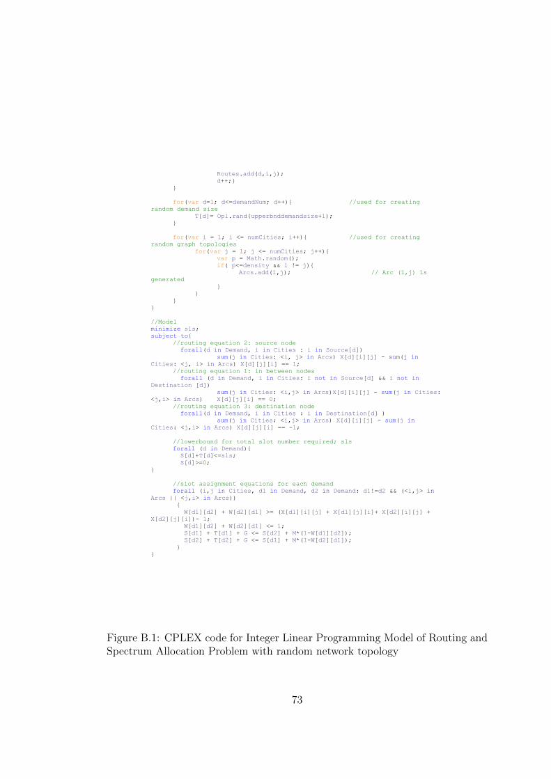
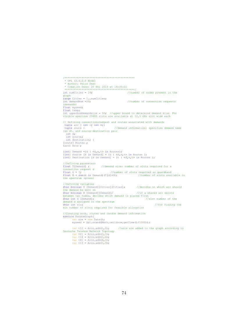
as reported by CPLEX is provided. CPLEX code for ILP model which creates

random demand attributes and random network topologies for different sparsity

levels and node numbers can be seen in Appendix B.1.

The performance analysis of our formulation for RSA without predefined set

of routes resulted that for fully connected networks (sparsity coefficient of 1), the

formulation can handle up to 100 commodities in 25 node networks, up to 50

42

Sparsity (F)

Demand Number (D)

Node Number (N)

Run Time (CPU Seconds)

Objective function value

1 4 8 0,02 43

1 10 8 0,06 89

1 30 8 173,90 97

1 50 8 3597,99 247

1 4 14 0,03 24

1 10 14 0,22 96

1 30 14 2,70 94

1 50 14 47,45 95

1 75 14 3600,97 (gap 2,32%)

1 4 25 0,06 46

1 10 25 0,61 49

1 30 25 7,92 47

1 50 25 29,77 48

1 75 25 81,84 49

1 100 25 850,48 49

1 4 50 0,41 79

1 10 50 3,03 78

1 30 50 34,91 91

1 50 50 118,67 47

1 75 50 3600,00 (gap 23,11%)

1 4 100 1,55 91

1 10 100 13,66 95

1 30 100 173,78 48

1 50 100 3600,00 (gap 48,07%)

Table 5.1: Test Results: Run Time and Objective Function Values for NetworkTopologies with Sparsity Coefficient 1 consisting of {8, 14, 25, 50, 100} nodes andtraffic load of {4, 10, 30, 50, 75, 100} Demands. Gaps reported at the objectivefunction values denote that the results could not be attained due to 3600 CPUseconds time limit.

43

Sparsity (F)

Demand Number (D)

Node Number (N)



0,75 4 8 0,02 75

0,75 10 8 0,36 91

0,75 30 8 3600,72 (gap 1,98%)

0,75 50 8 3599,55 (gap 5,03%)

0,75 75 8 3600,00 infeasible

0,75 4 14 0,03 47

0,75 10 14 0,38 84

0,75 30 14 8,39 48

0,75 50 14 1905,86 45

0,75 75 14 3600,00 (gap 1,08%)

0,75 4 25 0,14 34

0,75 10 25 1,16 47

0,75 30 25 20,97 48

0,75 50 25 29,69 48

0,75 75 25 322,59 49

0,75 100 25 3600,00 (gap 12,88%)

0,75 4 50 0,63 75

0,75 10 50 5,94 93

0,75 30 50 199,67 93

0,75 50 50 394,44 49

0,75 75 50 3600,00 (no LP file)

0,75 4 100 3,13 69

0,75 10 100 25,56 73

0,75 30 100 369,86 49

0,75 50 100 3600,00 (no LP file)

Table 5.2: Test Results: Run Time and Objective Function Values for NetworkTopologies with Sparsity Coefficient 0.75 consisting of {8, 14, 25, 50, 100} nodesand Connection Requests of {4, 10, 30, 50, 75, 100} Demands. Gaps reported atthe objective function values denote that the results could not be attained dueto 3600 CPU seconds time limit. “(no LP file)” at the objective function valuedenotes that the model file (.LP) could not be produced within 3600 CPU secondstime limit.

44

commodities in 8,14 and 50 node networks and up to 30 commodities in 100 node

networks (see Table 5.1). For networks with sparsity coefficient of 0.75, the formu-

lation can handle up to 10 commodities in 8 node networks, 50 commodities in 14

node networks, 75 commodities in 25 node networks, 50 commodities in 50 node

networks and 30 commodities in 100 node networks (see Table 5.2). For networks

with sparsity coefficient of 0.5, the formulation can handle up to 10 commodities

in 8 node networks, 30 commodities in 14 node networks, 75 commodities in 25

and 50 node networks and 30 commodities in 100 node networks (see Table 5.3).

For very sparse networks (sparsity coefficient 0.25), the formulation can handle

up to 75 commodities in 50 node networks and up to 30 commodities in 25 and

100 node networks, but due to small numbers of edges present for small network

topologies of 8 and 14 nodes, commodities beyond 30 result in infeasibility (see

Table 5.4). A summary of the amount of traffic handled for different node values

can be seen in Figure 5.1.

0,01

0,10

1,00

10,00

100,00

1000,00

10000,00

Ru

n T

ime

(CP

U S

eco

nd

s)

(D-N):Demand Number-Node Number Combination

Number of Commodities Handled vs Sparsity

Sparsity 1 Sparsity 0.75 Sparsity 0.5 Sparsity 0.25

Figure 5.1: Trend of Run Time Values for Demand Number-Node Number vsSparsity Combinations

The results show that changing sparsity levels has different impacts on run

times depending on the size of the network. Searching for an optimum value in

45

Sparsity (F)

Demand Number (D)

Node Number (N)



0,5 4 8 0,02 28

0,5 10 8 1,44 100

0,5 30 8 3600,52 (gap 8,45%)

0,5 50 8 3604,64 (gap 74,66%)

0,5 4 14 0,06 70

0,5 10 14 0,72 90

0,5 30 14 190,31 94

0,5 50 14 3594,68 (gap 9,71%)

0,5 4 25 0,08 42

0,5 10 25 0,86 44

0,5 30 25 6,52 46

0,5 50 25 82,61 48

0,5 75 25 528,05 48

0,5 100 25 3600,00 (gap 26,03%)

0,5 4 50 0,45 55

0,5 10 50 4,31 91

0,5 30 50 50,05 99

0,5 50 50 106,45 46

0,5 75 50 696,47 49

0,5 100 50 3600,00 (no LP file)

0,5 4 100 2,53 84

0,5 10 100 19,67 98

0,5 30 100 474,73 48

0,5 50 100 3600,00 (no LP file)

Table 5.3: Test Results: Run Time and Objective Function Values for NetworkTopologies with Sparsity Coefficient 0.5 consisting of {8, 14, 25, 50, 100} nodesand Connection Requests of {4, 10, 30, 50, 75, 100} Demands. Gaps reported atthe objective function values denote that the results could not be attained dueto 3600 CPU seconds time limit. “(no LP file)” at the objective function valuedenotes that the model file (.LP) could not be produced within 3600 CPU secondstime limit.

46

Sparsity (F)

Demand Number (D)

Node Number (N)



0,25 4 8 0,05 89

0,25 10 8 0,27 185

0,25 30 8 0,08 infeasible



0,25 100 8 0,72 infeasible

0,25 4 14 0,08 72

0,25 10 14 0,55 133

0,25 30 14 0,25 infeasible

0,25 50 14 0,77 infeasible

0,25 75 14 1,86 infeasible

0,25 100 14 3,50 infeasible

0,25 4 25 0,09 44

0,25 10 25 0,67 35

0,25 30 25 3,83 45

0,25 50 25 3600,00 (gap 6,87%)

0,25 75 25 3600,00 (gap 24,57%)

0,25 100 25 3600,00 (gap 52,63%)

0,25 4 50 0,31 85

0,25 10 50 3,83 86

0,25 30 50 28,06 98

0,25 50 50 58,67 49

0,25 75 50 597,72 49

0,25 100 50 3600,00 (gap 37,11%)

0,25 4 100 1,09 99

0,25 10 100 11,00 89

0,25 30 100 225,42 49

0,25 50 100 3600,00 (gap 35,23%)

Table 5.4: Test Results: Run Time and Objective Function Values for NetworkTopologies with Sparsity Coefficient 0.25 consisting of {8, 14, 25, 50, 100} nodesand Connection Requests of {4, 10, 30, 50, 75, 100} Demands. Gaps reported atthe objective function values denote that the results could not be attained dueto 3600 CPU seconds time limit.

47

fully connected networks (sparsity coefficient 1) produce better runtime values

compared to networks with average sparsity (0.75 and 0.5 sparsity coefficients)

at almost every demand-node number combination variation. For small network

topologies (8 and 14 node networks), increasing the connectivity of a graph both

decreases the average solution time and increases the maximum number of com-

modities that can be handled. Searching for a solution in very sparse networks

often results in infeasibility in small network topologies, when the number of

commodities exceed the number of nodes in the network (see Figure 5.2).

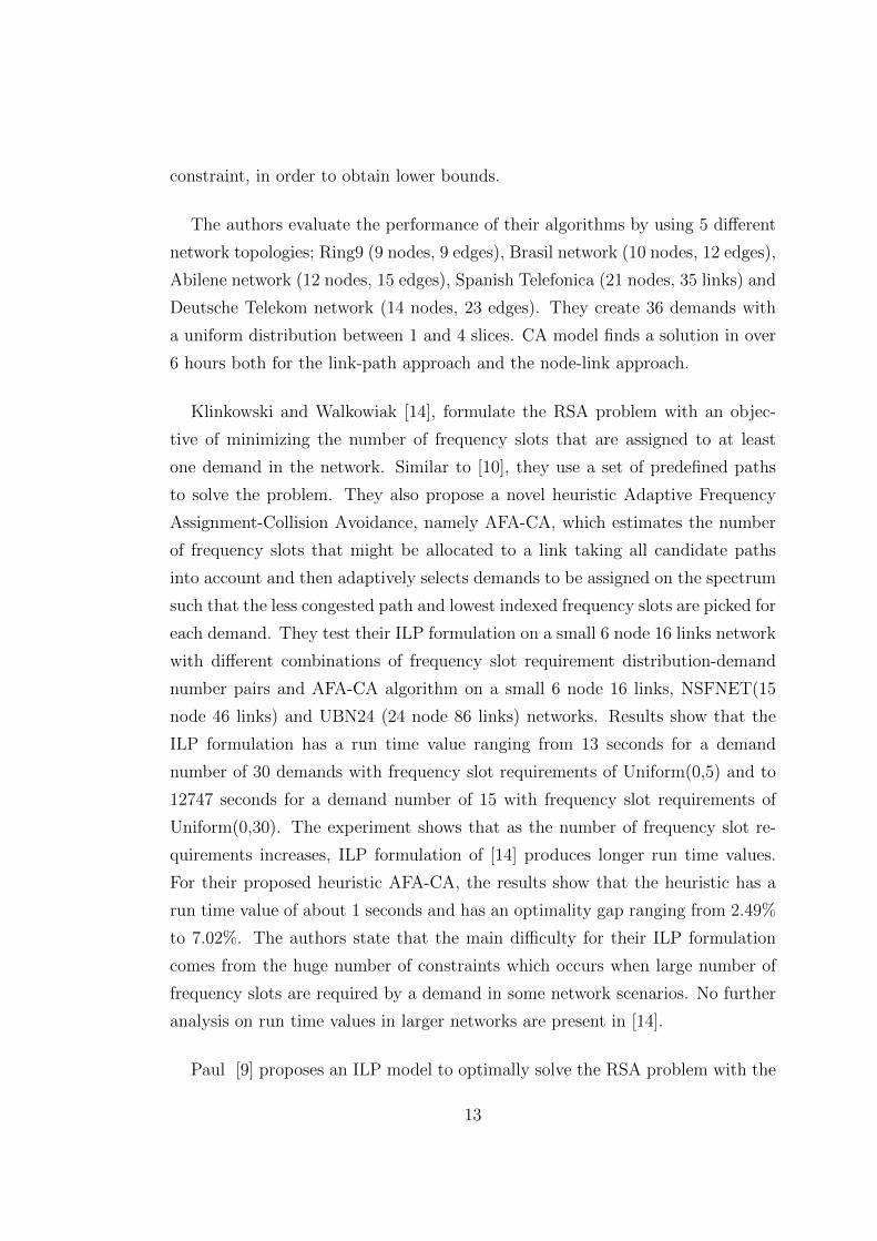
For network topologies larger than 25 nodes, behavior of solution times com-

pared to number of commodities to be handled show a different trend. For very

sparse networks and balanced number of commodity-node number combinations,

a solution is found faster compared to denser networks. However, as the number

of demands exceed the number of nodes in the network, a solution cannot be

found in 3600 seconds CPU time limit. Generally, performance of fully connected

graphs are better than average sparsity graphs at almost every number of connec-

tion requests, similar to the outcomes of small network topologies. (An exception

to this generalization occurs at 50 node network topology and 75 connection re-

quests (Figure 5.3), where networks with 0.5 sparsity coefficient results in faster

solutions than fully connected networks).

For 25 node network topology with connection request numbers almost equal

to or smaller than the number of nodes present in the graph, and for network

topologies beyond 50 nodes – except for fully connected graphs – increase in

connectivity does not yield in better run time values. (See Figures 5.3 and 5.4

for the graphic of trends of run times for network topologies beyond 25 nodes).

In fact, network topologies with 0.75 sparsity coefficient values result in highest

solution time values compared to 0.5 and 0.25 sparsity coefficients for network

topologies with nodes 25-50. One possible reason for this outcome may be the

decrease in amount of paths to be considered during routing and allocation phase

for networks with 0.5 sparsity coefficient than 0.75 sparsity coefficient. For 100

node networks, up to 10 demands the trend is similar to 25-50 node networks,

but from 30 demands and upwards, higher run time requirement shifts towards

sparser networks: 0.5 sparsity coefficient and below. The general trends of run

48

0,01

0,10

1,00

10,00

100,00

1000,00

10000,00


Ru

n T

ime

D-N

Run Time Comparison for 8 Node Network

4-8 10-8 30-8 50-8 75-8 100-8

0,01

0,10

1,00

10,00

100,00

1000,00

10000,00


Ru

n T

ime

D-N


4-14 10-14 30-14 50-14 75-14 100-14

Figure 5.2: Run Time Comparison of Different Sparsity Coefficients for SmallNetworks Consisting of 8 and 14 Nodes49

0,01

0,10

1,00

10,00

100,00

1000,00

10000,00


Ru

n T

ime

D-N


4-25 10-25 30-25 50-25 75-25 100-25

0,10

1,00

10,00

100,00

1000,00

10000,00


Ru

n T

ime

D-N


4-50 10-50 30-50 50-50 75-50 100-50

Figure 5.3: Run Time Comparison of Different Sparsity Coefficients for NetworksConsisting of 25 and 50 Nodes 50

1,00

10,00

100,00

1000,00

10000,00


Ru

n T

ime

D-N


4-100 10-100 30-100 50-100 75-100 100-100

Figure 5.4: Run Time Comparison of Different Sparsity Coefficients for LargeNetworks Consisting of 100 Nodes

51

time values according to number of commodities, number of nodes present in the

networks and network sparsity can be seen in Figures 5.5, 5.6, 5.7 and 5.8.

Figure 5.5 gives the effects of changing demand value-node value combinations

on run time values for fully connected networks. Figure 5.6 gives the effects of

changing demand value-node value combinations on run time values for networks

with 75% connectivity and Figures 5.7 and 5.8 represent networks with 50% and

25% connectivity, respectively.

410

30

50

410

30

50

75

410

30

50

75

100

410

30

50

75

410

30

50

0,00

500,00

1000,00

1500,00

2000,00

2500,00

3000,00

3500,00

4000,00

0

20

40

60

80

100

120

Ru

n T

ime

(C

PU

Se

con

ds)

Demand Number-Node Number

RunTime Values for Sparsity Coefficient=1

D N RunTime

Figure 5.5: Effects of increasing connection requests on run time values at variousnetwork topologies for fully connected networks

52

410

30

50

75

410

30

50

75

410

30

50

75

100

410

30

50

75

410

30

50

0,00

500,00

1000,00

1500,00

2000,00

2500,00

3000,00

3500,00

4000,00

0

20

40

60

80

100

120

Ru

n T

ime

(C

PU

Se

con

ds)


RunTime Values for Sparsity Coefficient=0.75

D N RunTime

Figure 5.6: Effects of increasing connection requests on run time values at variousnetwork topologies for sparsity coefficient of 0.75

53

410

30

50

410

30

50

410

30

50

75

100

410

30

50

75

100

410

30

50

0,00

500,00

1000,00

1500,00

2000,00

2500,00

3000,00

3500,00

4000,00

0

20

40

60

80

100

120

Ru

n T

ime

(C

PU

Se

con

ds)


RunTime Values for Sparsity Coefficient=0.5

D N RunTime


54

4 10

30

50

75

100

4 10

30

50

75

100

4 10

30

50

75

100

4 10

30

50

75

100

4 10

30

50

0,00

500,00

1000,00

1500,00

2000,00

2500,00

3000,00

3500,00

4000,00

4-8

10

-8

30

-8

50

-8

75

-8

10

0-8

4-1

4

10

-14

30

-14

50

-14

75

-14

10

0-1

4

4-2

5

10

-25

30

-25

50

-25

75

-25

10

0-2

5

4-5

0

10

-50

30

-50

50

-50

75

-50

10

0-5

0

4-1

00

10

-10

0

30

-10

0

50

-10

0

0

20

40

60

80

100

120

Ru

n T

ime

(C

PU

Se

con

ds)


RunTime Values for Sparsity Coefficient=0.25D N RunTime


55

5.2 Results for a Real Network Topology:

Deutsche Telekom Network

To test the performance of our proposed ILP model and heuristic algorithms,

Deutsche Telekom Network is chosen as a real-life network topology. Deutsche

Telekom (DT) Network consists of 14 nodes and 23 edges and the map of the

DT graph can be seen in Figure 5.9. Computational tests are conducted on DT

Figure 5.9: Deutsche Telekom Network

network for D = {12, 15, 20, 25, 27} traffic loads. For each traffic load d ∈ D,

5 instances are created with demand sizes generated from the distribution Uni-

form(0,50). CPLEX code for ILP model which creates random demand attributes

on DT network topology can be seen in Appendix B.2. Run time values of ILP,

LCS algorithm and ICPA algorithm are calculated for traffic loads with identical

56

demand attributes (source, sink and demand sizes). The results of the experi-

ments can be seen in Table 5.5. The first three columns in Table 5.5 gives the

instance, node number in the graph and the demand number used as traffic load.

“ILP Run Time” column gives the solution time values for the ILP formulation

in CPU seconds. “LCS Algorithm Run Time” and “ICPA Algorithm Run Time”

columns denote the run time values in CPU seconds to obtain a solution from LCS

and ICPA algorithms respectively. “ILP Objective Value” column gives the exact

solution values (or the gap from optimality declared by CPLEX) and “LCS Al-

gorithm Objective Value” and “ICPA Algorithm Objective Value” columns give

the solution values of the heuristic algorithms. “LCS Gap” and “ICPA Gap”

columns are the optimality gaps of heuristic solutions from the exact solution

of ILP. To calculate the percentage gaps in the last two columns, formulas of“LCSAlgorithmObjectiveV alue”

“ILPObjectiveV alue”− 1 and “ICPAAlgorithmObjectiveV alue”

“ILPObjectiveV alue”− 1 are used.

INSTANCE

NETWORK TOPOLOGY (DEUTSCHE TELEKOM)

DEMAND NUMBER (D)

ILP RUN TIME LCS ALGORITHM

RUN TIME

ICPA ALGORITHM

RUN TIME ILP OBJ VALUE

LCS ALGORITHM OBJ VALUE

ICPA ALGORITHM OBJ VALUE

LCS GAP ICPA GAP

1 14 12 1,96 0,24 0,51 75 99 90 32,00% 20,00%

2 14 12 2,33 0,22 0,42 76 129 103 69,74% 35,53%

3 14 12 0,76 0,17 0,33 46 66 52 43,48% 13,04%

4 14 12 1,77 0,22 0,38 61 96 95 57,38% 55,74%

5 14 12 2,31 0,19 0,35 78 122 122 56,41% 56,41%

1 14 15 3,80 0,23 0,51 61 82 73 34,43% 19,67%

2 14 15 4,60 0,21 0,50 80 95 94 18,75% 17,50%

3 14 15 29,59 0,21 0,46 76 101 101 32,89% 32,89%

4 14 15 28,84 0,26 0,53 79 109 114 37,97% 44,30%

5 14 15 7,85 0,23 0,44 76 76 110 0,00% 44,74%

1 14 20 885,87 0,35 0,52 75 103 117 37,33% 56,00%

2 14 20 28,32 0,29 0,77 116 132 117 13,79% 0,86%

3 14 20 1974,20 0,26 0,68 106 194 130 83,02% 22,64%

4 14 20 28,61 0,33 0,66 87 138 135 58,62% 55,17%

5 14 20 315,88 0,37 0,49 64 111 118 73,44% 84,38%

1 14 25 117,52 0,35 0,86 112 156 130 39,29% 16,07%

2 14 25 2028,93 0,43 0,93 122 208 202 70,49% 65,57%

3 14 25 3253,70 0,38 0,80 138 175 146 26,81% 5,80%

4 14 25 1301,89 0,38 0,86 90 145 133 61,11% 47,78%

5 14 25 809,84 0,44 0,94 110 199 187 80,91% 70,00%

1 14 27 960,59 0,46 1,01 151 197 277 30,46% 83,44%

2 14 27 3685,07 0,47 1,06 124

(gap23,58%) 180 136 45,16% 9,68%

3 14 27 3602,06 0,41 0,83 105 (gap 8,65%) 170 156 61,90% 48,57%

4 14 27 3602,78 0,39 0,85 115 (gap 21,05%) 181 162 57,39% 40,87%

5 14 27 3601,81 0,40 0,96 95 (gap 13,83%) 152 144 60,00% 51,58%

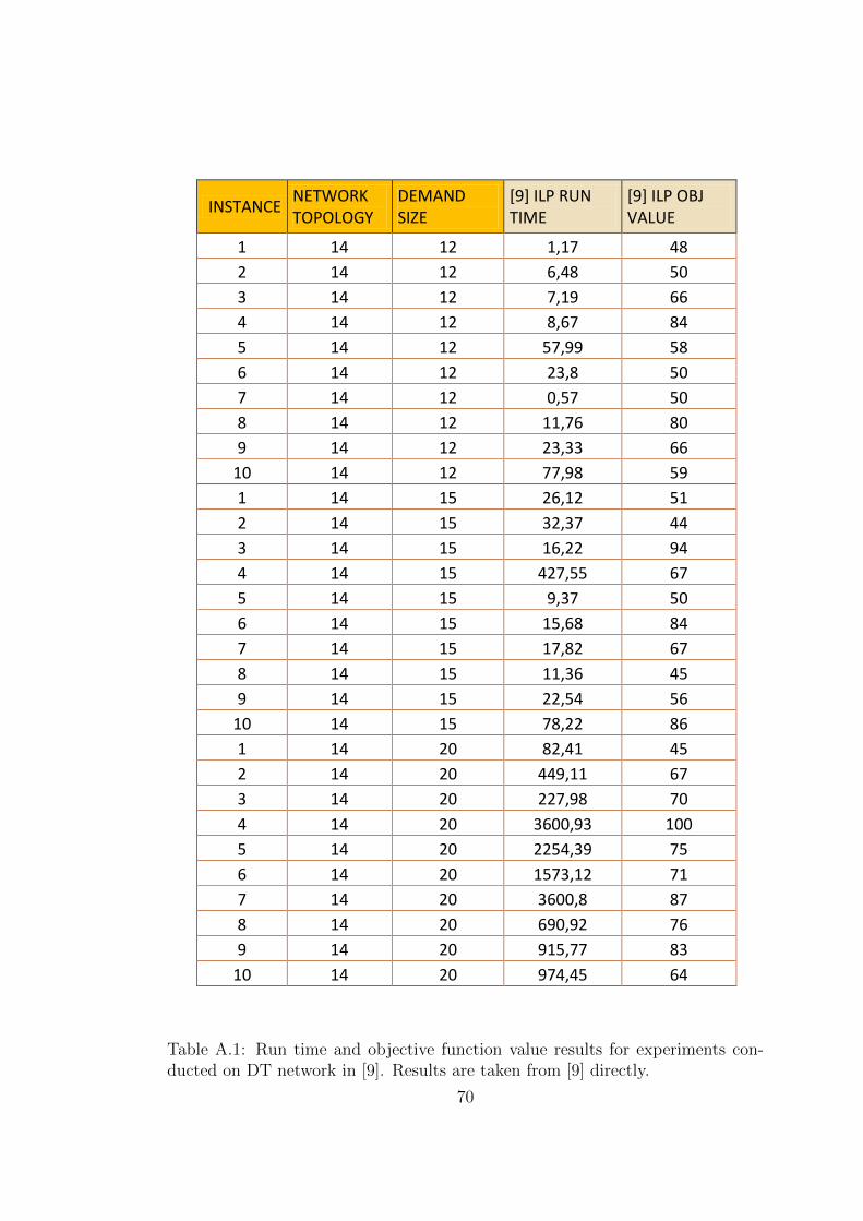
Table 5.5: Test Results: Run Time and Objective Function Values for DeutscheTelekom Network Topology with Connection Requests of 12,15,20,25 and 27 De-mands

57

5.2.1 Performance Analysis for ILPcurrentwork and Heuristic

Algorithms

To test the performance of our proposed ILP formulation, we used test scenarios

with the same dimensions as [9]: Deutsche Telekom network topology and D =

{12, 15, 20} traffic loads. [9]’s experiments show that the average run time values

are 21,89 seconds for 12 demands, 65,73 seconds for 15 demands and 896,02

seconds for 20 demands (detailed values for ILP[9] can be seen in Appendix A.1,

results that took more than 3600 seconds are excluded while calculating average

solution times). The formulation of [9] could not produce solutions for demands

beyond 25. As there is no further information on the source, sink and demand

size values for the demands used in instances, we could not test the performance

of [9]’s and our ILP formulation on the same set of demands; hence we use the

average run time values for comparison purposes. Results of performance analysis

on Deutsche Telekom Network showed that our formulation can find quite fast

solutions compared to [9] in the same dimension of network topology and total

demand numbers. As an outcome of our computational tests, we can see that our

formulation has lower average run time values compared to [9] and it can also

produce solutions for 25 commodities within 3600 CPU seconds time limit.

Only 1 out of 5 instances resulted in a solution within 3600 seconds for 27

commodities, hence the upper bound that our formulation can produce solutions

on Deutsche Telekom network is determined as 25 commodities. Computational

results show that average run times for low load cases (demand numbers up to 20

commodities) are within executable limits and solutions can be obtained on ILOG

CPLEX. For high load cases (demand numbers from 20 commodities and beyond)

ILP formulation can still produce results within 3600 CPU time limit boundaries

up to 25 commodities. A summary table of the results in Table 5.5 consist-

ing of average run time comparisons for ILPcurrentwork and heuristic algorithms

can be seen in Table 5.6 and Figure 5.10 shows the graphical representation of

ILPcurrentwork, Least Cost Slot and Iterative Common Path Allocation algorithm

values.

58

DEMAND NUMBER

AVERAGE RUN TIME ILP_currentwork (CPU SECONDS)

AVERAGE LCS ALGORITHM RUN TIME (CPU SECONDS)

AVERAGE ICPA ALGORITHM RUN TIME (CPU SECONDS)

Average Gap from Optimality LCS

Average Gap from Optimality ICPA

12 1,83 0,21 0,40 51,80% 36,14%

15 14,93 0,23 0,49 24,81% 31,82%

20 646,58 0,32 0,62 53,24% 43,81%

25 1502,38 0,40 0,88 55,72% 41,04%

27 3090,46 0,43 0,94 50,98% 46,83%

Table 5.6: Comparison of average run time values for ILP Formulations andHeuristic Algorithms for demand loads of 12, 15, 20, 25 and 27 commodities.

As a result of computational tests, it can be stated that our ILP formula-

tion, ILPcurrentwork, finds a solution faster than the formulations proposed by [9]

and [10] and also can produce results for higher loads of traffic.

Heuristic algorithms LCS and ICPA find solutions very fast compared to ILP

formulation, however there are large gaps from optimality for both algorithms.

From the results it can be seen that LCS or ICPA cannot be used for finding close

solutions to optimum results on their own, but can produce good initial solutions

for the ILP model in order to limit initial search and to reduce run time values.

In the next section, we analyze the impact of providing initial solutions obtained

from our proposed heuristic algorithms to our ILP formulation.

59

12 15 20 25 27

Average Run Time ILP 1,83 14,93 646,58 1502,38 3090,46

Average Run Time LCS 0,21 0,23 0,32 0,40 0,43

Average Run Time ICPA 0,40 0,49 0,62 0,88 0,94

0,10

1,00

10,00

100,00

1000,00

10000,00R

un

Tim

e (

CP

U S

eco

nd

s)

Demand Number

Figure 5.10: Average run time of ILP Formulation and Heuristic Algorithms fortraffic loads of 12, 15, 20, 25 and 27 commodities.

5.2.2 Performance Analysis for LCS+ILP and ICPA+ILP

In this section, we design an alternative experiment to test the effects of provid-

ing an initial solution to ILOG CPLEX on achieving the optimum solution. We

use DT network topology and the exact same source-sink and demand size values

used in the previous section as inputs for ILP model and heuristics+ILP model

combinations. In order to be able to use the same data sets with the previous

section as inputs for Matlab and ILOG, we used Excel as an interface between

these two programs. In Table 5.7, “ILP Run Time(CPU Seconds)” column gives

the solution time value for the ILP model where the attributes of demand; source,

sink and demand size values are created internally in the model definition. The

values in this column are the values in Table 5.5 and are included in this ta-

ble for comparison of the effects of defining demand attributes internally in a

model file versus externally through an Excel file. “ILP Run Time (input from

Excel)” column gives the solution time value for the same ILP model except

60

with the difference that the same demand attributes are read from an Excel file.

“LCS+ILP Run Time” column gives the solution time for the model where a

solution is found by LCS algorithm and it is read as an initial solution along with

the demand attributes from an Excel file by the ILP model, and “ICPA+ILP Run

Time” column gives the solution time for the model where a solution is found

by ICPA algorithm and it is read as an initial solution along with the demand

attributes from an Excel file by the ILP model. “ILP Obj Value”, “LCS+ILP

Obj Value”, “ICPA+ILP Obj Value” columns give the objective function val-

ues achieved by the models in “ILP Run Time (input from Excel)”, “LCS+ILP

Run Time”, “ICPA+ILP Run Time” columns. The last two columns denote the

decrease in run time values for Heuristic+ILP combinations. Note that all for

ILP(input from Excel), LCS+ILP and ICPA+ILP columns, demand attributes

are read from the Excel file; hence the percentage decrease in run time values

are in reference to ILP(input from Excel), not the ILP formulation results in the

first column where demand attributes are defined internally in the model. For

instances of demand number 27, reading data from Excel increases the run time

drastically (beyond 7000 seconds), hence in the objective function value of these

instances, we provide percentage gaps from optimality reported by CPLEX at

3600 CPU seconds in the respective objective function value columns.

61

INSTANCE

NETWORK TOPOLOGY (DEUTSCHE TELEKOM)

DEMAND NUMBER (D)

ILP RUN TIME (CPU Seconds)

ILP RUN TIME (input from

Excel)

LCS+ ILP RUN TIME (CPU Seconds)

ICPA+ILP RUN TIME (CPU Seconds)

ILP OBJ VALUE LCS+ILP OBJ

VALUE ICPA+ILP OBJ

VALUE

LCS+ILP Decrease in

Run Time (%)

ICPA+ILP Decrease in

Run Time(%)

1 14 12 1,96 3,58 1,98 2,78 75 75 75 44,69% 22,35%

2 14 12 2,33 3,80 4,30 2,24 76 76 76 -13,16% 41,05%

3 14 12 0,76 1,16 0,25 0,91 46 46 46 78,45% 21,55%

4 14 12 1,77 2,35 1,02 0,77 61 61 61 56,60% 67,23%

5 14 12 2,31 3,27 1,55 1,53 78 78 78 52,60% 53,21%

1 14 15 3,80 4,08 3,03 3,42 61 61 61 25,74% 16,18%

2 14 15 4,60 3,37 2,04 4,42 80 80 80 39,47% -31,16%

3 14 15 29,59 101,19 50,25 47,75 76 76 76 50,34% 52,81%

4 14 15 28,84 25,28 26,98 31,69 79 79 79 -6,72% -25,36%

5 14 15 7,85 9,91 4,34 4,73 76 76 76 56,21% 52,27%

1 14 20 885,87 2112,52 361,52 660,53 75 75 75 82,89% 68,73%

2 14 20 28,32 453,92 239,51 397,12 116 116 116 47,24% 12,51%

3 14 20 1974,20 2759,08 954,63 1932,38 106 106 106 65,40% 29,96%

4 14 20 28,61 78,19 79,72 45,62 87 87 87 -1,96% 41,65%

5 14 20 315,88 685,99 493,91 301,84 64 64 64 28,00% 56,00%

1 14 25 117,52 227,27 209,75 191,99 112 112 112 7,71% 15,52%

2 14 25 2028,93 3138,75 1890,11 2218,51 122 122 122 39,78% 29,32%

3 14 25 3253,70 5466,21 3943,32 3075,28 138 138 138 27,86% 43,74%

4 14 25 1301,89 3619,25 2043,55 2371,58 90 90 90 43,54% 34,47%

5 14 25 809,84 2952,38 1358,09 1814,53 110 110 110 54,00% 38,54%

1 14 27 960,59 7000+ 7000+ 7000+ gap 40,52% gap 40,13% gap 42,11% - -

2 14 27 3685,07 7000+ 7000+ 7000+ gap 35,43% gap 34,13% gap 34,4% - -

3 14 27 3602,06 7000+ 7000+ 7000+ gap 13,21% gap 8,49% gap 8,49% - -

4 14 27 3602,78 7000+ 7000+ 7000+ gap 28,12% gap 20,69% gap 20,69% - -

5 14 27 3601,81 7000+ 7000+ 7000+ gap 31,25% gap 31,24% gap 36,63% - -

Table 5.7: Test results of run time values for ILP and heuristic algorithms anddecrease in run time values for heuristics+ILP combinations. Demand loads of12, 15, 20, 25 and 27 commodities are used for tests. Run time value 7000+ meansthat the results took more than 7000 CPU seconds and were automatically killedby the system.

62

From the results in the Table 5.7, it can be seen that the run time values

between “ILP Run Time” and “ILP Run Time (input from Excel)” columns are

different, but the objective function values in Tables 5.7 and 5.5 are the same. The

reason for the difference in run time values is that in the “ILP Run Time(CPU

Seconds)” column, demand attributes (source, sink and demand size values) are

created as internal data by execute command, but in “ILP Run Time (input from

Excel)” the same demand sets with identical source, sink and demand size values

are read from Excel as external data. Reading data from an internal source

vs. from an external .dat source such as Excel creates differences in terms of

run times, as “internal data elements are pulled from OPL as needed and are

not allocated any memory” but “external data elements are pushed to OPL and

allocated memory whether it is used by the model or not” [15].

Although reading data from Excel increases run time values, providing an

initial solution found via heuristic algorithms LCS and ICPA to the ILPcurrentwork

on ILOG decreases run time values significantly. Note that at each iteration, the

same objective function value is found for ILP, LCS+ILP and ICPA+ILP. A

summary table of average run time values for ILP models with data pulled from

“internal” and “external” sources and initial solutions provided by LCS and ICPA

algorithms as well as average percentage decrease in run time values can be seen

in Table 5.8.

DEMAND NUMBER

Average Run Time ILP_currentwork (CPU Seconds)

Average Run Time ILP_currentwork (input from Excel)

Average Run Time LCS+ILP (CPU Seconds)

Average Run Time ICPA+ILP (CPU Seconds)

Average Decrease in Run Time LCS+ILP

Average Decrease in Run Time ICPA+ILP

12 1,83 2,83 1,82 1,65 35,73% 41,88%

15 14,93 28,77 17,33 18,40 39,76% 36,03%

20 646,58 1217,94 425,86 667,50 65,03% 45,19%

25 1502,38 3080,77 1888,96 1934,38 38,69% 37,21%

Table 5.8: Test results of average run time values for ILP and heuristic algorithmsand percentage decrease in run time values for heuristics+ILP combinations.

Despite the fact that ICPA gives solutions closer to the optimum than LCS, for

larger network topologies than 15 nodes, the solution obtained from LCS provides

a better initial solution for the ILP model than ICPA in terms of the percentage

of decrease in run time. For small network topologies (12 nodes and less), solving

63

the problem on CPLEX already provides fast solutions; hence applying a heuristic

for an initial solution is not necessary. In general, the combination of LCS+ILP

provides an average of 44.8% decrease in run time and ICPA+ILP gives an average

of 40% decrease when compared to solving the problem on CPLEX directly.

As reading the data from Excel increased the solution times beyond 7000 CPU

seconds for traffic loads of 27 and higher, we provide the percentage optimality

gap reported by CPLEX at 3600 CPU seconds. From the results of traffic load of

27, it can be concluded that LCS+ILP combination decreases optimality gap by

an average of 2,77% and ICPA+ILP decreases the optimality gap by an average

of 1,24% around 3600 seconds. Although not tested within this thesis, a further

investigation can be made on the percentage decrease in run times for traffic loads

beyond 27 when initial solutions are defined manually in CPLEX formulation as

internal data, rather than reading them externally from Excel. Another possible

area of research could be the combination of AFA-CA heuristic algorithm of [14]

with our proposed ILPcurrentwork and to test the run time values for higher traffic

loads.

12 15 20 25

Average Run Time LCS+ILP 1,82 17,33 425,86 1888,96

Average Run Time ICPA+ILP 1,65 18,40 667,50 1934,38

Average Run Time ILP (Excel) 2,83 28,77 1217,94 3080,77

1,00

10,00

100,00

1000,00

10000,00

Ru

n T

ime

(C

PU

Se

con

ds)

Demand Number

Figure 5.11: Graph of average run time with an initial solution provided:LCS+ILP and ICPA+ILP algorithms.

64

Chapter 6

Conclusion

The development of OFDM technology in optical networks provides huge spec-

trum efficiencies while transmitting connections and offers a novel area of inter-

disciplinary research for many branches of engineering. Motivated by the possible

improvements on application of graph theory on OFDM based fiber optic net-

works, we investigate the Routing and Spectrum Allocation problem in optical

networks in this thesis. We consider two cases: in one setting, allocation to the

spectrum are made by taking a set of precomputed routes into consideration and

in the other setting, we span the whole solution space without taking a predefined

set of routes into consideration. We present an improved formulation for the RSA

problem with predefined set of paths and propose a novel global formulation, RSA

without predefined set of paths, that reaches to the global optimum.

We use 7 different computational experiment settings to test the performance

of our ILP formulation and heuristic algorithms. In our settings, we use 5 differ-

ent network topologies consisting of N={8, 14, 25, 50, 100} nodes–each generated

randomly for every iteration. We test for the limitations of traffic load that can

be handled on these networks and also test the effect of using different sparsity

levels for network topologies and their impact on achieving a solution in terms

of longevity of run time values. In the last 2 sets of experiments, we use a real-

life network topology–Deutsche Telekom network consisting of 14 nodes and 23

65

edges– to test the amount of traffic load that can be handled and the speed of

our ILP formulation. We also test the run time and results generated by our

proposed heuristic algorithms, LCS and ICPA, on DT network topology. Lastly,

we examine the amount of decrease on run time values when an initial solution

from the results we obtain from our heuristic algorithms is provided as an input

to our ILP formulation.

From the performance analysis tests we have conducted, it can be concluded

that our ILP formulation provides faster solutions compared to formulations that

have run time analyses in literature and also it can process much larger networks

with higher traffic loads. Our heuristic algorithms could not produce results as

close to optimal solution as desired, but the hybrid formulation of LCS+ILP and

ICPA+ILP create an average of 44% and 40% decrease in run time values of our

ILP formulation, which provides opportunity for exploration of larger networks

and denser traffic loads.

There is no previous work in literature that investigates the effects of sparsity

of graphs on distribution of demands in optical networks. As a result of our

experimental analysis on sparsity of optical networks, it can be stated that solving

RSA problem on fully connected networks generally produces better outputs. For

very sparse networks where around 25% of all connections are present compared

to fully connected networks, increasing traffic load often yields in infeasibility. For

networks with average connectivity, having a network with 50% of all connections

present generally yields in faster solutions when compared to 75% of edges being

present.

For further study, we propose extensions to the Routing and Spectrum Alloca-

tion problem. AFA-CA algorithm of [14] provides solutions with small optimality

gaps. For high traffic networks and large networks, combining AFA-CA’s initial

solutions to our ILPcurrentwork that finds the global optimum on static fiber op-

tic networks could produce global solutions faster than our proposed algorithms.

As an additional study, it would be interesting to investigate possible solution

methods for the dynamic RSA problem, with demands allocated on spectrum as

connection requests arrive into the system.

66

Bibliography

[1] CiscoSystems, “Fundamentals of dwdm technology.” http://docstore.

mik.ua/univercd/cc/td/doc/product/mels/cm1500/dwdm/dwdm\

textunderscoreovr.htm. Accessed: March, 2016.

[2] NewportCorporation, “Fiber optic basics.” http://www.newport.com/

Tutorial-Fiber-Optic-Basics/978863/1033/content.aspx. Accessed:

March, 2016.

[3] O. Gerstel, I. Cisco, et al., “Elastic optical networking: A new dawn for the

optical layer?,” IEEE Communications Magazine, vol. 50, no. 2, pp. 12–20,

February 2012.

[4] M. Jinno, H. Takara, B. Kozicki, et al., “Distance-adaptive spectrum re-

source allocation in spectrum-sliced elastic optical path network,” IEEE

Communications Magazine, vol. 48, no. 8, pp. 138–145, August 2010.

[5] M. Jinno, H. Takara, and B. Kozicki, “Concept and enabling technologies of

spectrum-sliced elastic optical path network (slice),” Communications and

Photonics Conference and Exhibition (ACP), pp. 1–2, November 2009.

[6] M. Jinno, H. Takara, and B. Kozichi, “Dynamic optical mesh networks:

drivers, challenges and solutions for the future,” Proceedings of ECOC, pp. 1–

5, 2009.

[7] M. Jinno, H. Takara, B. Kozichi, Y. Tsukishima, and Y. Sone, “Spectrum-

efficient and scalable elastic optical path network: Architecture, benefits and

enabling technologies,” IEEE Communications Magazine, vol. 47, pp. 66–73,

2009.

67

[8] M. Jinno, H. Takara, and B. Kozichi, “Filtering characteristics of highly-

spectrum efficient spectrum-sliced elastic optical path (slice) network,” Pro-

ceedings of OFC, p. JWa43, 2009.

[9] P. Arijit, “An optimal and a heuristic approach to solve the route and spec-

trum allocation problem in ofdm networks,” Master’s thesis, University of

Windsor, 2014.

[10] K. Christodoulopoulos, I. Tomkos, and E. Varvarigos, “Routing and spec-

trum allocation in ofdm-based optical networks with elastic bandwidth allo-

cation,” IEEE Global Telecommunications Conference (GLOBECOM 2010),

pp. 1–6, 2010.

[11] K. Christodoulopoulos, I. Tomkos, and E. Varvarigos, “Elastic bandwidth

allocation in flexible ofdm-based optical networks,” Journal of Lightwave

Technology, vol. 29, no. 9, pp. 1354–1366, 2011.

[12] Y. Wang, X. Cao, and Y. Pan, “A study of the routing and spectrum allo-

cation in spectrum-sliced elastic optical path networks,” INFOCOM, 2011

Proceedings IEEE, pp. 1503–1511, 2011.

[13] I. Velasco, M. Klinkowski, M. Ruiz, and J. Comellas, “Modeling the routing

and spectrum allocation problem for flexgrid optical networks,” Photonic

Network Communications, vol. 24, no. 3, pp. 177–186, 2012.

[14] M. Klinkowski and K. Walkowiak, “Routing and spectrum assignment in

spectrum sliced elastic optical path network,” IEEE Communications Let-

ters, vol. 15, no. 8, pp. 884–886, 2011.

[15] IBMKnowledgeCenter, “Initialization and memory allocation.”

http://www.ibm.com/support/knowledgecenter/SS6MYV_3.5.0/ilog.

odms.ide.odme.help/Content/Optimization/Documentation/ODME/

_pubskel/ODME_pubskels/startall_ODME35_Eclipse1276.html. Ac-

cessed: July, 2016.

68

Appendix A

Tables

69

INSTANCE NETWORK TOPOLOGY

DEMAND SIZE

[9] ILP RUN TIME

[9] ILP OBJ VALUE

1 14 12 1,17 48

2 14 12 6,48 50

3 14 12 7,19 66

4 14 12 8,67 84

5 14 12 57,99 58

6 14 12 23,8 50

7 14 12 0,57 50

8 14 12 11,76 80

9 14 12 23,33 66

10 14 12 77,98 59

1 14 15 26,12 51

2 14 15 32,37 44

3 14 15 16,22 94

4 14 15 427,55 67

5 14 15 9,37 50

6 14 15 15,68 84

7 14 15 17,82 67

8 14 15 11,36 45

9 14 15 22,54 56

10 14 15 78,22 86

1 14 20 82,41 45

2 14 20 449,11 67

3 14 20 227,98 70

4 14 20 3600,93 100

5 14 20 2254,39 75

6 14 20 1573,12 71

7 14 20 3600,8 87

8 14 20 690,92 76

9 14 20 915,77 83

10 14 20 974,45 64

Table A.1: Run time and objective function value results for experiments con-ducted on DT network in [9]. Results are taken from [9] directly.

70

Appendix B

Code

71

/*********************************************

* OPL 12.6.0.0 Model

* Author: Pelin Öner

* Creation Date: 18 Ekim 2015 at 14:04

*********************************************/

int numCities =100; //number of nodes present in the graph

range Cities = 1..numCities;

int demandNum =30; //number of connection requests

(demands)

float density= 0.5; //sparsity coefficient

float myseed;

int upperbnddemandsize = 50; //upper bound to determine demand size. For

visible spectrum 25600 slots are available at 12,5 GHz slot wide each

// Defining connections(edges) and routes associated with demands

tuple arc { int i; int k;}

tuple route { //demand information: specifies demand name

(as d), and source-destination pair

int d;

int source;

int destination; }

{route} Routes ;

{arc} Arcs ;

{int} Demand ={d | <d,s,t> in Routes};

{int} Source [d in Demand] = {s | <d,s,t> in Routes };

{int} Destination [d in Demand] = {t | <d,s,t> in Routes };

//Defining parameters

float T[Demand] ; //demand size: number of slots required for a

connection request d

float G = 1; //number of slots required as guardband

float M = sum(d in Demand)(T[d]+G); //number of slots available in

the spectrum (given)

//Defining variables

dvar boolean X [Demand][Cities][Cities]; //decides on which arc should

the demand be sent on

dvar boolean W [Demand][Demand]; //if a shared arc exists

between two nodes, decides which demand is placed first

dvar int S [Demand]; //slot number of the

demand d assigned in the spectrum

dvar int sls; //for finding the

min number of slots required for feasible allocation

//Creating random arcs, routes and demand information

execute RandomGraph{

var now = new Date();

myseed = Opl.srand(Math.ceil(now.getTime()/1000));

var d = 1; //this part is used for

creating connection requests with random information

while(d<=demandNum){

var i = Opl.rand(numCities+1);

var j = Opl.rand(numCities+1);

if(i!=j && i!=0 && j!=0){

72

Routes.add(d,i,j);

d++;}

}

for(var d=1; d<=demandNum; d++){ //used for creating

random demand size

T[d]= Opl.rand(upperbnddemandsize+1);

}

for(var i = 1; i <= numCities; i++){ //used for creating

random graph topologies

for(var j = 1; j <= numCities; j++){

var p = Math.random();

if( p<=density && i != j){

Arcs.add(i,j); // Arc (i,j) is

generated

}

}

}

}

//Model

minimize sls;

subject to{

//routing equation 2: source node

forall(d in Demand, i in Cities : i in Source[d])

sum(j in Cities: <i, j> in Arcs) X[d][i][j] - sum(j in

Cities: <j, i> in Arcs) X[d][j][i] == 1;

//routing equation 1: in between nodes

forall (d in Demand, i in Cities: i not in Source[d] && i not in

Destination [d])

sum(j in Cities: <i,j> in Arcs)X[d][i][j] - sum(j in Cities:

<j,i> in Arcs) X[d][j][i] == 0;

//routing equation 3: destination node

forall(d in Demand, i in Cities : i in Destination[d] )

sum(j in Cities: <i,j> in Arcs) X[d][i][j] - sum(j in

Cities: <j,i> in Arcs) X[d][j][i] == -1;

//lowerbound for total slot number required; sls

forall (d in Demand){

S[d]+T[d]<=sls;

S[d]>=0;

}

//slot assignment equations for each demand

forall (i,j in Cities, d1 in Demand, d2 in Demand: d1!=d2 && (<i,j> in

Arcs || <j,i> in Arcs))

{

W[d1][d2] + W[d2][d1] >= (X[d1][i][j] + X[d1][j][i]+ X[d2][i][j] +

X[d2][j][i])- 1;

W[d1][d2] + W[d2][d1] <= 1;

S[d1] + T[d1] + G <= S[d2] + M*(1-W[d1][d2]);

S[d2] + T[d2] + G <= S[d1] + M*(1-W[d2][d1]);

}

}

Figure B.1: CPLEX code for Integer Linear Programming Model of Routing andSpectrum Allocation Problem with random network topology

73

/*********************************************

* OPL 12.6.0.0 Model

* Author: Pelin Öner

* Creation Date: 20 Eki 2015 at 16:35:22

*********************************************/

int numCities = 14; //number of nodes present in the

graph

range Cities = 1..numCities;

int demandNum =20; //number of connection requests

(demands)

float myseed;

float temp;

int upperbnddemandsize = 50; //upper bound to determine demand size. For

visible spectrum 25600 slots are available at 12,5 GHz slot wide each

// Defining connections(edges) and routes associated with demands

tuple arc { int i; int k;}

tuple route { //demand information: specifies demand name

(as d), and source-destination pair

int d;

int source;

int destination; }

{route} Routes ;

{arc} Arcs ;

{int} Demand ={d | <d,s,t> in Routes};

{int} Source [d in Demand] = {s | <d,s,t> in Routes };

{int} Destination [d in Demand] = {t | <d,s,t> in Routes };

//Defining parameters

float T[Demand] ; //demand size: number of slots required for a

connection request d

float G = 1; //number of slots required as guardband

float M = sum(d in Demand)(T[d]+G); //number of slots available in

the spectrum (given)

//Defining variables

dvar boolean X [Demand][Cities][Cities]; //decides on which arc should

the demand be sent on

dvar boolean W [Demand][Demand]; //if a shared arc exists

between two nodes, decides which demand is placed first

dvar int S [Demand]; //slot number of the

demand d assigned in the spectrum

dvar int sls; //for finding the

min number of slots required for feasible allocation

//Creating arcs, routes and random demand information

execute RandomGraph{

var now = new Date();

myseed = Opl.srand(Math.ceil(now.getTime()/1000));

var t12 = Arcs.add(1,2); //arcs are added to the graph according to

Deutsche Telekom Network Topology

var t21 = Arcs.add(2,1);




74


































var t1210 = Arcs.add(12,10);

var t1012 = Arcs.add(10,12);

var t1213 = Arcs.add(12,13);

var t1312 = Arcs.add(13,12);

var t1314 = Arcs.add(13,14);

var t1413 = Arcs.add(14,13);

var t1410 = Arcs.add(14,10);

var t1014 = Arcs.add(10,14);

var d = 1; //this part is used for

creating connection requests with random information

while(d<=demandNum){

var i = Opl.rand(numCities+1);

var j = Opl.rand(numCities+1);

if(i!=j && i!=0 && j!=0){

Routes.add(d,i,j);

d++;}

}

for(var d=1; d<=demandNum; d++){ //used for creating

random demand size

T[d]= Opl.rand(upperbnddemandsize+1);

}

}

75

//Model

minimize sls;

subject to{

//routing equation 2: source node

forall(d in Demand, i in Cities : i in Source[d])

sum(j in Cities: <i, j> in Arcs) X[d][i][j] - sum(j in

Cities: <j, i> in Arcs) X[d][j][i] == 1;

//routing equation 1: in between nodes

forall (d in Demand, i in Cities: i not in Source[d] && i not in

Destination [d])

sum(j in Cities: <i,j> in Arcs)X[d][i][j] - sum(j in Cities:

<j,i> in Arcs) X[d][j][i] == 0;

//routing equation 3: destination node

forall(d in Demand, i in Cities : i in Destination[d] )

sum(j in Cities: <i,j> in Arcs) X[d][i][j] - sum(j in

Cities: <j,i> in Arcs) X[d][j][i] == -1;

//lowerbound for total slot number required; sls

forall (d in Demand){

S[d]+T[d]<=sls;

S[d]>=0;

}

//slot assignment equations for each demand

forall (i,j in Cities, d1 in Demand, d2 in Demand: d1!=d2 && (<i,j> in

Arcs || <j,i> in Arcs))

{

W[d1][d2] + W[d2][d1] >= (X[d1][i][j] + X[d1][j][i]+ X[d2][i][j] +

X[d2][j][i])- 1;

W[d1][d2] + W[d2][d1] <= 1;

S[d1] + T[d1] + G <= S[d2] + M*(1-W[d1][d2]);

S[d2] + T[d2] + G <= S[d1] + M*(1-W[d2][d1]);

}

}

Figure B.2: CPLEX code for Integer Linear Programming Model of Routing andSpectrum Allocation Problem with Deutsche Telekom Network Topology

76

Date post:	22-Feb-2022
Category:	Documents
Upload:	others
View:	7 times
Download:	0 times

ROUTING AND SPECTRUM ALLOCATION IN STATIC FIBER OPTIC …

Documents