NASA Reference Publication 1091 June 1982 Global Differential Geometry An Introduction for Control Engineers RP ! 109 i B. F. Doolin and C. F. Martin https://ntrs.nasa.gov/search.jsp?R=19820022028 2018-06-16T05:07:32+00:00Z
Transcript
NASA Reference Publication 1091
June 1982
Global Differential Geometry An Introduction for Control Engineers
Equivalence Classes of Curves ........................ The Tangent Space in General ......................... Mapping Between Tangent Spaces ........................
VECTOR FIELDS AND THEIR ALGEBRA ........................ VectorFields ................................ Derivations ................................. A Digression on Notation ........................... Isopmorphism Between Vector Fields and Derivations .............. The Algebra of Vector Fields and Lie Derivations .... . .......... An Example of Lie Algebra ..........................
LIE GROUPS, GROUP ACTIONS AN'D LIE ALGEBRAS ................... LieGroups .................................. GroupAction ................................. One-Parameter Subgroups and Vector Fields .................. Examples From the Symplectic Group ......................
GRASSMANNIAN MANIFOLDS AND THE RICCATI EQUATICN ................ Linear Optimal Control ............................ The Grassmannian ...............................
A simple example .............................. ThesubspaceWA .............................. ThechartsP(W) .............................. ThemanifoldsGP(V) ............................
An Application of the Grassmannian ....................... The Riccati Equation ............................. Some Properties of the Riccati Equation ................... Theorem ...................................
GLOBAL DIFFERENTIAL GEOMETRY - AN INTRODUCTION FOR CONTROL ENGINEERS
B. F. Doolin* and C. F. Martin**
Ames Research Center
This publication has been written to acquaint engineers, especially control engineers, with the basic concepts and terminology of modern global differential geometry. The ideas discussed are applied here mainly as an introduction to the Lie theory of differential equations and to the role of Grassmannians in control systems analysis. To reach these topics, the fundamental notions .of manifolds, tangent spaces, vector fields, and Lie algebras are discussed and exemplified. An appendix reviews such concepts needed for vector calculus as open and closed sets, compactness, continuity, and derivative.
Although the content is mathematical, this is not a mathematical treatise. Several excellent introductions to modern differential geometry exist, but they are written for readers with a strong mathematical, rather than engineering, background. Reading this publication should help an engineer to read those treatises, as well as to understand the points, if not the detailed arguments, of research papers on geometric control, and many of those on nonlinear control.
INTRODUCTION
This report presents some basic concepts, facts of global differential geometry, and some of its uses to a control engineer. It is not a mathematical treatise; the subject matter is well developed in many excellent books, for example, in refer- ences 1, 2, and 3, which, however, are intended for the reader with an extensive mathematical background. Here, only some basic ideas and a minimum of theorems and proofs are presented. Indeed, a proof occurs only if its presence strongly aids understanding. Even among basic ideas of the subject, many directions and results have been neglected. Only those needed for viewing control systems from the stand- point of vector fields are discussed.
Differential geometry treats of curves and surfaces, the functions that define them, and transformations between the coordinates that can be used to specify them. It also treats the differential relations that stitch pieces of curves or surfaces together or that tell one where to go next.
In thinking of functions that can define surfaces in space, one is likely to think of real functions (functions assigning a real number to a given point of their argument) of three-space variables such as the kinetic energy of a particle, or the distribution of temperature in a room. Differential geometry examines properties inherent in the surfaces these functions define that, of course, are due to the sources of energy or temperature in the surroundings. Or, given enough of these functions, one might use them as proper coordinates of a problem. Then the generali- ties of differential geometry show how to operate with them when they are used, for example, to describe a dynamic evolution.
*Currently with Computer Sciences Corporation, Mountain View, California. **Senior National Research Council Associate. Currently with Case Western
Reserve University, Cleveland, Ohio.
Differential geometry, in sum, derives general properties from the study of func- tions and mappings so that methods of characterization or operation can be carried over from one situation to another. Global differential geometry refers to the description of properties and operations that are good over "large" portions of space.
Though the studies of differential geometry began in geodesy and dynamics where intuition can be a faithful guide, the spaces now in this geometry's concern are far more general. Instead of considering a set of three or six real functions on a space of vectors of three or six dimensions, spaces can be described by longer ordered strings of numbers, by sets of numbers ordered in various ways, by ordered sets of products of numbers. Examples are n-dimensional vector spaces, matrices, or multi- linear objects like tensors. It is not just these sets of numbers, but also the rules one has of passing from one set to another that form the proper subject matter of differential geometry, and which link it to matters of interest in control.
All analytic considerations of geometry begin with a space filled with stacks of numbers. Before one can proceed to discuss the relations that associate one point with another or dictate what point follows another, one has to establish certain ground rules. The ground rules that say if one point can be distinguished from another, or that there is a point close enough to wherever you want to go, are referred to as topological considerations. The basic description of the topological spaces underlying all the geometry of this paper is given in an appendix on fundamen- tals of vector calculus. This appendix discusses such desired topological character- istics as compactness and continuity, which is needed to preserve these characteris- tics in passing from one space to another. The appendix concludes by recalling two theorems from vector calculus that provide the basic glue by which manifolds, the word for the fundamental spaces of global differential geometry, are assembled. Since this discussion is fundamental to differential geometry, we briefly review it. The review is relegated to an appendix, however, because it is not the topic of this paper, nor should one dwell on it.
The first two sections of the body of the paper describe manifolds, the spaces of our geometry. Some simple manifolds are mentioned. Several definitions are given, starting with one closest to intuition then passing to one perhaps more abstract, but actually less demanding to verify in cases of interest in control engineering. Then mappings between manifolds are considered. A special space, the tangent space, is discussed in section 3. A tangent space is attached to every point in the manifold. Since this is where the calculus is done, it and its relations to neighboring tangent spaces and to the manifold that supports it must be carefully described.
Computation in these spaces is the topic of the next two sections. Calculus on manifolds is given in section 4 on vector fields and their algebra, where the connec- tion between global differential geometry and linear and nonlinear control begins to become clear. Section 5, with its treatment of some algebraic rules, concludes our exposition of the fundamentals of the geometry.
The examples given as the development unfolds should not only help the reader understand the topic under discussion, but should also provide a basic set for testing ideas presented in the current literature. More comprehensive applications of differ- ential geometry to control are given in the final major section of the paper.
2
MANIFOLDS AND THEIR MAPS
The first part of this section is devoted to the concept of a manifold. It is defined first by a projection then by a more useful though less intuitive definition. Finally, it is seen how implicitly defined functions give manifolds. Examples are considered both to enhance intuition and to bring out conceptual details. The idea of a manifold is brought out more clearly by considering mappings between manifolds. The properties of these mappings occupy the last part of this section.
Differentiable Manifolds
Although the detailed global description of a manifold can be quite complicated, basically a differentiable manifold is just a topological space (X,Q), that in the neighborhood of each point looks like an open subset of ak. (In the notation (X,0), X is some set and 52 consists of all the se s defined as open 'n X and that char- acterize its topology. As to the notation 61 E , each point in di k is specified as an ordered set of k real numbers. These and other notions arising below are discussed in the appendix.) This description can be formalized into a definition:
A subset M of en is a k-dimensional manifold if for each x E M there are: open subsets U and V of Rn with x EU, and a diffeomorphism f from U to V such that:
f(U n M) = {y E v : yk+' = . . . = yn = 01
Thus, a point y in the image of f has a representation like:
Y = (yl(x>, y2(x>, . . *, Yk(X> 9 0, * * * 0)
d . A straight line is a simple example of a one-dimensional manifold, a manifold in It is a manifold in 6@ even if it is given, for example, in G2. There it might
represent the surface of solutions of the equation of a particle of unit mass under no forces: ;i = 0 and with given initial momentum: x(t = 0) = a. In the coordinate system y1 = x; y2 = x - a, the manifold is
63 iven by the points (y,,O). To the par-
ticle, its whole world looks like part of part of a2.
though we see its tracks clearly as Any open subset of the straight line is also a one-dimensional manifold,
but a closed subset of it is not.
The sphere in Q3 is an example of a two-dimensional manifold. of a closed manifold and is often denoted as S2.
It is an example Thus, for a point P in e3:
p = (X1,X2,X3), the manifold is given as the set:
S2 = {P E IQ3 : x'1 + xf + xi - 1 = O]
Its two-dimensional character is clear when a point in S2 is given in terms of two variables, say, latitude and longitude. Another map of S2 into 6Z2 is given by stereographic projections. Since this map not only has historical interest but also will be used later, it will now be discussed to show that S2 is a two-dimensional manifold.
Let U(r;P) be an r-neighborhood of a given point P of St3 in M=S2 such that U n M is the set
3
UnM={P:x;+x;+x;-110; x: + x2 Z e(1 + x3) ; e > 01
Then define the stereographic projection of a point P into the plane as the function from U r7 M to 613:
f e,P = (Ulr u2, 0) = ( Xl X2
1 - x3 ' 1 - x3 9 0 )
The mapping is illustrated in sketch (a), where the following ratios
P= (Xq,JQ,X3)
Sketch (a)
can be seen to hold: u2/x2 = d/R and R/d = (1 - x3)/l. The projection is generated by drawing a line from the "North Pole" (O,O,l) to a point on the sphere and continu- ing the line to the plane x3 = 0. Thus, a point of the sphere is associated with a point on the plane and vice versa.
The map is written fe,P to call attention to the important role that the parameter e plays in restricting its domain of definition. With the restriction, f can be shown to be a diffeomorphism; without it, the function is not.
The one function is not enough to map the whole manifold. The point (O,O,l) and some e neighborhood of it on the manifold have been excluded. Another similar map that includes these points but excludes others can be given by a stereographic pro- jection from the "South Pole"
( Xl x2
g e,P = 1+x3'1+x3 , 0 >
with g,,P defined on the set
{P: x'1 +x;+x;-l=O; xf + XI 2 e(1 - x3) ; e > 01
4
If the parameter e is given the value unity, f maps the lower hemisphere and g maps the upper hemisphere onto the interior of the unit circle on the plane that coincides with the plane x3 = 0. Agreeably, the points of the sphere where x3 = 0 go into the same points of u1 and u2 under both maps.
The examples of one- and two-dimensional manifolds so far have been sets given in some 6in and mapped into I@ or 6X2. Sets forming manifolds are not always described naturally in some an. To embed them in an Rn before showing that the definition is satisfied may be an undesirably awkward task. In fact, it is not necessary, and we will extend our previous definition so as to avoid it. That labor, however, will be avoided only at the expense of our introducing more formalism now.
Let M be a second countable, Hausdorff topological space. A chart.in M is a pair @,a) with V an open set and CL a C" function onto an open set in 6? and having a C" inverse. A C" atlas is a set of such charts, ((Vi,ai)} = A, with the following properties:
(3 M =uVi
(ii) If (Vl,a,) and (V,,a,) are in A and
V, n V, # 4, then
-1 a2a1 : CQ(V, n v,> -+ a2(v1 n v2)
isa C" diffeomorphism.
Sketch (b), which illustrates the subsets V, and V2 and maps aid in picturing the content of condition (ii). With this formalism second definition of a manifold can now be given:
A C" manifold is a pair (M,A) where M is the second countable Hausdorff topological space, and A is a maximal C" atlas.
~1~ and o2 may established, our
Sketch (b)
5
The conditions on the topology guarantee that the number of charts required to cover M is countable. The word "maximal" gives a technical condition. It makes the atlas the class of collections of just enough charts to form a countable basis of charts. By referring to the class, one is not tied to a representation given by a particular set of charts.
Although the definition seems unduly complicated, it turns out to be just what is necessary to meet our intuition. Every m-dimensional manifold determined by the definition can in fact be considered as a subset of 6%* for some n:m 5 n < 2m + 1. Any weakening of the definition can allow objects which cannot be embedded in some 6P .
We opened this discussion of differentiable manifolds with the remark that basi- cally a differentiable manifold is a topological space that in the neighborhood of each point looks like an open subset of 6ik. The first definition said that each neighborhood, even though expressed as a subset of din, was equivalent to 6ik. That is; the space expressed in din really only had k, not n, degrees of freedom. Another way of saying this is by saying that a k-dimensional manifold can be expressed using n variables with n-k conditions imposed on them.
These remarks are made because in practice , manifolds are often given as the set of points where a certain function vanishes. The implicit function theorem gives conditions under which the vanishing of the function gives k constraints (exchanging the k and n-k of the previous paragraph), so that only n-k of the variables are free, and the space is a manifold with dimensions n-k if the theorem is satisfied everywhere. Then the manifold is said to be given implicitly, or by the implicit function theorem.
Formalizing the abgve remarks, we consider a Cc" function F with domain A c An and range in di . in- A, the function
That is, for every choice of n real numbers (xl,...,xn) F has the k real numbers F = (f,,...,fk). Let M be the
set
M = (x : F(x) = 0 = (O,O,...,O)}
If the rank of the Jacobian matrix F' is equal to k for all x E M, then M is an n-k-dimensional manifold.
Under the conditions stated, the implicit function theorem says that k of the variables can be expressed in terms of the other n-k, and the latter can be given values arbitrarily. Another statement of the implicit function theorem (see ref. 4, pg. 43) shows that a coordinate transformation can be found that assigns the value zero to the k explicit functions. In other words, the conditions of the first definition of a manifold are satisfied.
Examples
Consider the real function F = alxl + a2xg + a3x3 - b = 0. It is clear that alxl + a2x2 + a3x3 - b = 0 describes a plane, a two-dimensional manifold, in a3. It is not difficult to imagine a change of coordinates that reorients 6S3 so that every point in the given plane can be written as (y1,y2,0), satisfying the first definition for a two-dimensional manifold. One also sees that the Jacobian matrix of F is F' = (a l,a2,a3) which has rank one for all x in F(x) = 0. The implicit function theorem, then, says the manifold is of dimension 3 - 1 = 2.
6
Another example of using the implicit function theorem is given by the two- dimensional manifold S2. Here F = x21 + X; + x:- 1 = 0, and F' = (2x1,2x2,2x3). Now, F' is not zero because not all xi vanish simultaneously, for F = 0 is not satisfied by x1 = x2 = x3 = 0. Thus, F' has rank one and the manifold S2 has dimension 3 - 1 = 2.
Let a second condition be imposed on the space. For instance, consider the circle resulting from passing a plane containing the origin through S2. In particu- lar, consider the function
F = (f,,f,) :' 6X3 + 6%'
with f, as before,
fl = x1 z+x;+x;-150
and
f, = x1 - ax2 = 0
The manifold M = {x : F = 01 is the circle S1. The Jacobian matrix of F is:
2x1 2x, 2x3 F' =
1 -a 0
the rank of which is two everywhere on the manifold. The dimension of this manifold, therefore, equals 3 - 2, or 1.
On the other hand, consider the function G : 6x3 -f R1 defined by:
G(xl,x2,x3) = xf + x; - xi
The zero set of G is a cone. But note that the rank of G' is 0 at (O,O,O). Thus, at this point the cone doesn't satisfy the condition for the implicit function theorem, 6?2.
our definition of a manifold, or our intuitive view of its being locally like
To exercise our second definition of a manifold, let us consider S2 again with charts defined as follows:
Vl = 1(x 1,X2,X3) : X3 # 11
V2 = {(x1,x2,x3) : x3 # -11
c%l(x1,x2’x3) = (upu2) = ( x1 x2
1 - x3 ' 1 - x3 >
a2(xl,x2,x3) = (vlsv2 >= (l:lx 3
x2 ) '1+x,
7
Then the set
A = {(V,, al>, (V2 ,a2) I
satisfies the first condition for an atlas. Consideration of the geometry of the stereographic projection shows that hl and a2 , with their domains restricted appro- priately actually map onto R2 and are one to one. Also,
al(V1 n V2> = a2 - {(O,O)l = a2(V1 n V2)
where a2 - {(O,O)] means that the point (0,O) has been deleted from H2. Further- more, after calculating the inverse:
( u’1 + u; ’ Uf + u; > Sin:: its partial derivatives exist and are continuous whenever (ul,uz) # (O,O), a2a1 isa C" diffeomorphism. That a similar calculation yields the same conclu- sion for -1
ala2 confirms that A is an atlas.
Thus, S2 satisfies our new definition of a manifold. In fact, a little thought makes one realize that any space that is a manifold by the first definition is also one by the second. Furthermore, anything given as a manifold by the implicit function theorem satisfies both definitions.
Another, trivial but important, example of a class of manifolds is afforded by any open subset of din. There the atlas may consist of the set itself together with the identity map. Thus, the notion that manifolds are spaces that locally look like open subsets of An is at least self-consistent. This example is important because the whole idea of the definition of manifolds is to be able to see how calculations valid in 6in carry over into any other manifold.
Another example of a manifold, which is an open set of Euclidean space and which is important in systems theory, follows. Let
x=Ax+bu
be a single-input controllable system. Recall that controllability is equivalent to having the rank of the matrix
[b,Ab,A2b, . . . . An-lb]
equal to n where A is an n x n matrix. Now let M be the set of pairs (A,b) such that a system is controllable: M = {(A,b) : G = Ax + bu is controllable]. The complement of this set is the set that satisfies the condition:
det[b,Ab,A'b, . . . . An-lb] = 0
8
Since this is a closed set in & n2-tn , the set M is open in 61n2+n and therefore is a manifold.
The system, being of single input, is a special case. In general, when the con- trol distribution function B is an n x m matrix, M* is also a manifold where M* is the set:
M* = ((A,B) : 2 = Ax + Bu is controllable}
Although the conditions are more involved and less easy to describe than the deter- minant condition above a similar argument shows that the controllable pairs are an open subset of 6p W-4 .
A more general example along these same lines is the set of triples of matrices (A,B,C) representing the system
. x=Ax+Bu
y = cx
If the system is controllable and observable, it can be shown that this set of triples is also an open subset of a suitable Euclidean space.
Related to this manifold is a set of matrix transfer functions T(s). These are matrices of rational functions that arise as the Laplace transforms of the above sys- tems. Whether this set {T(s)) i s a manifold is a deep question in systems theory. It has been answered affirmatively by Martin Clark (ref. 5) and Roger Brockett (ref. 6), and independently by Michiel Hazewinkel (ref. 7) and by Christopher Byrnes and N. Hurt (ref. 8). Much of the study in linear systems is involved with various properties of this manifold.
Manifold Maps
We have described manifolds and seen a few examples of them. Now we can describe the requirements on functions that allow them to be maps between manifolds.
A function f,
f: M+N
is a manifold map if for every xEM and chart (V,a) with x E V, there is a chart (U,B) for N with f(V) C U such that the composite function Bofoa-':
80foa -1 : a(V) + B(u)
is a Coo diffeomorphism. The relations are illustrated in sketch (c) for f = A,, the map in the following example.
As an example, let M = N = S2. Let A be a matrix such that I = ATA, an orthogonal transformation. Then, if x E S2,
/AxI' = (Ax)- (Ax) = xTATAx = xTx = 1
Sketch (c)
Thus, A maps S2 onto S2. Consider a specific A, namely A,:
A, =
and let a and B be the previous stereographic projection aI. become for a:
and
2% xl = v,(l - x3) =
vg + vf + 1
2V2 x2 =
v; + v; + 1
v; + v; - 1 x3 =
v; + v; + 1
Those relations
The map A, gives E = Alx:
% = + (x1 + x2)
10
x2 = - l (-x1 + 4 LT
z3 = x3
and @Aa-' maps (v1,v2) + (ul,u2) thus:
-1 1 Xl + x2
ul=l - =- - x3 l (VI + 3)
)/y 1-x3 =x
x2 1 -x1 + x2 Ul = 1
- l (-1 + v2) =- - x3 fi 1 - x3 Lz
Both a and f3 are C" functions on their respective domains. The composite map (v1,v2) -f (ul,u2) is also clearly CO". The map A,, therefore is a manifold map.
Thus, orthogonal transformations are manifold maps. They also form a manifold. The set of n x n orthogonal matrices form an (n/2)(n - 1) dimensional manifold. The truth of this statement will be verified by using the implicit function theorem.
The defining relation of an orthogonal matrix can be used to give a function of the matrices into the zero set:
f(X) = XTX -I=0
It must now be shown that the rank of the derivative is constant over all elements of the set. The derivative at X = A can be found through the definition:
Rim IIHll+o
[f(x + HI - f(x) - f'(X)(H)lXzA = 0
where the differential f'(A)(H) recognizes that the derivative evaluated at A isa linear operator on H. Performing the expansion and considering the limit gives for the differential:
f ' (A) (HI = HTA + ATH
Now A is invertible by definition and therefore, in.the n x n case, maps one-to- one onto Rn2. Any matrix H is thus the image of some matrix under A, and one can write H + AH. The derivative then gives:
f'(A)(AH) = HT + H
Thus, the range of the derivative is seen to be the set of symmetric nxn matrices, which implies that it has the constant rank (n/2)(n + 1). Following the considera- tions of the implicit function theorem, the orthogonal nxn matrices form an (n/2) (n - 1)-dimensional manifold.
A final consideration for this section is that of forming manifolds from the Cartesian products of manifolds. If we have a manifold M with atlas A, we can construct a new manifold:
11
M x M = {(X,Y) : x,y E Ml
from M and A. The charts are constructed from the charts of A in the natural way as products, i.e., if @,,a,) and (V,,a,) are charts in A, then a chart for M x M is given by (V, x V,, a1 x a2) where
(al X a2> (X,Y> = (a,(X),a,(Y))
TANGENT SPACES
The previous section defined manifolds and gave several examples of them. This section considers a basic construction of one manifold from another. While the method of construction itself is of interest insofar as it illustrates general proce- dures of modern differential geometry, the particular result, the tangent space, is an object of great importance: it is by way of the tangent space that calculus can be done in general situations.
To gain familiarity with the idea of a tangent space, it will be worthwhile to spend some time with an example, that of the tangent space to the sphere. The infor- mation in the previous section concerning charts for the sphere will allow charts to be constructed for this new space. The atlas resulting from the construction will be examined in the light of the earlier definitions to see that this tangent space forms a manifold. The example is useful, too, for giving insight into such things as the dimensionality of a tangent space and the fact that its maps preserve its linear and differentiable structure. Part of the problem of constructing an atlas is that a map must be inverted and that its composition with another map is a diffeomorphism. Reducing our example from a sphere to a circle will simplify this calculation considerably.
Next, still preparatory to considering the general construction of a tangent space, the notion of equivalence classes of curves on a manifold, and their addition and scalar multiplication will be explored. This study provides the guide to the constructions that follow, and to the confirmation that the tangent space is a manifold.
The rest of the section will be devoted to the tangent space in general. It will be seen to be a manifold whose charts and chart maps are derived from those of the underlying manifold. It will be seen to have vector space properties. Similar properties of maps between tangent manifolds will be examined. The differentiating properties of these induced maps will be noted.
The Tangent Space of S2
Consider an object moving on S2, the surface of a sphere in space. As it moves, it generates a velocity vector which is tangent to the sphere at each point. Since it is tangent, the velocity vector lies in the tangent plane at each point and moves continuously through tangent planes as the object moves smoothly along the sphere. The concepts of a set of tangent planes and of smoothly transitioning from one to another is made precise by endowing the set of tangent planes together with their points of attachment with a manifold structure. That the set of tangent planes thus generates a manifold will be shown in two ways. The first uses the implicit function
12
theorem. The second constructs charts and chart maps explicitly and shows that the chart maps have the requisite properties. This explicit construction reveals the relation of tangent spaces to derivative operations on the manifolds from which they are obtained.
Let the sphere, S2, be described by the equation
x: + Xf + x; = 1
and let the charts and chart maps be as given in the previous section. plane to S2 at i7 = (x1,x2,x3) is the set
This is the space of vectors orthogonal to the radius vector (x1,x2,x3) and trans- lated to the origin. The manifold structure is obvious since there are two equations, one for the sphere, and the other for the tangent plane. That is, T(S2), is just the following set of points of 19~:
Since not all the xi vanish simultaneously, the rank of the matrix is 2 everywhere. The dimension of the manifold, therefore, is 4, corresponding to 2 degrees of freedom on the sphere, and 2 additional degrees of freedom on the plane tangent to the sphere at any point.
Now, if the object were moving freely in space (a3) and not constrained to the surface of the sphere, it would have three degrees of freedom of position. Its velocity vector, being unconstrained, would also have three degrees of freedom. As a manifold, then, the tangent space would be made up of two copies of 6Z3. That is to say, the tangent space of a3, T(ti3>, is the Cartesian product space R3 x ti3. If the object is considered to move in some open subset u of G3, then the space needed to describe all its possible positions and velocities is U x a3. In this case, T(U) = U x 6X3.
Return to considering motion on the sphere. section we know that S2
From the chart maps of the previous is locally like 6X2. It would be reasonable to suppose,
then, that the tangent space of S2 should look locally like G2 x 6?2 as will be confirmed by the calculations investigated in the following paragraphs. The calcula- tions will consider a curve, c, on the sphere. To learn what is to be meant by the tangent, or velocity, of the curve at some point on the sphere, we will calculate the velocity of the image of the curve in R2 The image of c in G2
, where we know what a tangent to a curve is. is obtained through the chart ma of course. Inspecting the
form of the calculation of the tangent to the curve in 61 !P will show that it is the image of the tangent of the curve in the manifold under a mapping given by the deriva- tive of the chart map. This inspection leads to the definition of the tangent to the curve on the manifold, and to the isolation of the map that maps it into e2.
13
Let c be a curve on the sphere; that is, c(t) is the position of a point at t, where t is an element of an open interval in 62l, and t = 0 is likewise in this interval. If it isn't, define a translation of 152~ so that the zero does occur there. Furthermore, define the translation so that c(0) = X0. Let (U,C$) be a chart containing c(0). The chart map transforms the curve c(t) by the composition 9.0 c into a curve in 6x2. The velocity vector of @OC is just the derivative with respect to time: (d/dt)$b c. It would be reasonable to expect that a chart map of the tangent space, T(S2), map the velocity vector of c into the velocity vector of (I 0 c. Now, the derivative of $I 0 c at t = 0 is just:
$ (4 o c> (0) = (0 0 c)’ (0) = 0’ (X,>c’ (0)
since the derivatives in question are defined. Thus, the velocity vectors c' are mapped by the derivative $I' of the chart map to elements of the "local" tangent space (9 0 c)'. Take, for example, the chart map 0:
then 4' is the matrix:
1 Xl 1 0 -
X3 (1 - x312
0 1 X2
1 - X3 (I - x3)2 .
A reasonable candidate for a chart in the tangent space T(S2) is then [T(U),T$(x,y)]:
= 1 + x3 ' 1 + x3 ' 1 + x3 - (1 + x3)2 ' 1 + x3 - (1 + x312 1 For proof that these charts and maps form an atlas, it must be shown that the
union of the sets T(U) and T(V) covers the tangent space, and that compositions of
14
one map with the inverse of the other over common domains of definition lead to Cc* maps. It is clear that the first condition is satisfied, that T(S2) = T(U) u T(V). The remainder of the argument is tedious and will be carried out only for the circle, for which it will be seen that [T(u),T$] and [T(v),TY] actually form an atlas.
Although computing the composition map of, for example, T$o(Ty>-'(a,g) is tedious, it is important to note that the outcome has the form
T+(Ty)-'($6) = [+y-'(&@,L(z)6]
where L(Z) is an invertible linear transformation for each a in the domain. Thus, the composite map preserves both the differentiable structure of the tangent space and its linear structure.
The computations are T
articularly simple for the circle, S1, which will be obtained by restricting S to the plane xl = 0. S1 will be mapped onto 6Z1 by $I and y where the image of X = (x2,x3) will be ul and vl, respectively. of the tangent in S1, 7 = (y,,y,>, will be u2 and v2, respectively. S1
The image is the set:
{(Tz,T): x; + xi - 1 = 0; x2y2 + x3y3 = 0)
Under the chart maps 4,~:
x2 = @G) = 1 _ x ; v1 = y(Z) =
x2 u1
3 1 + x3
The Jacobian matrices at (E,y) are:
9’ (3 = ( 1 _1 x , x2 1 ( 1 -X2
; 3 (1 - x312 y'(E) = 1 + x3 ' (1 + x3)2
>
giving the tangent vectors in 6?:
y2 x2y3 x2y3 UP = O'(x)7 = 1 _ x + ; VP
3 (1 - x3)2
= y' (X)7 = 1 Z', - 3 (1 + x3)2
To compute I$-~(u,) and y-'(v,) requires use of x; + x; - 1 = 0. One finds:
2% 2Vl 2 Ul -1 1-v; x2 = = ; x3 = =
Uf + 1 vf + 1 u; + 1 vf + 1
for points in the domain common to 9 and y.
and To compute (~')-1(ul,u2) and (y')-1(vl,v2) requires use of both 8: + xi - 1 = 0 X2Y2 + X3Y3 = 0. One finds:
Finally, the composition T$o(Ty)-l(V) = [$o~-~(V), #'~(y')'l(i?)] can be found to be:
1 -V2 -1 ul=-; u2z2= Vl Vl
TV2 Vl
These expressions give a diffeomorphism, since the point u1 =,vl = 0 is excluded as not being in the images of U n V. Note that u2 is given by a linear transformation at V.
Equivalence Classes of Curves
The example of a tangent space started with a sphere and a plane tangent to the sphere at a point. This plane was seen to contain the tangent to the velocity of a curve passing through .the point of attachment. As a matter of fact, the plane is the locus of tangents to all the curves on the surface at the point, a curve being a map of an interval of 6X1 into some region of the manifold. The interval of the real line is so adjusted for discussion that t = 0 corresponds to the point p of the manifold: c(0) = p. The curves can be grouped into classes. Being a tangent vector is taken to be a class property, and the tangent plane can be determined by a set of independent tangent vectors.
The classes are equivalence classes. Two curves are in the same class if they are equivalent to each other. They are equivalent if they pass through the same point and have the same velocity there. The velocity is measured in the local Euclidean frame given by the chart map attached at the point. Thus, the curves cl(t) and c2(t) are equivalent if
This equality is also written as
(@ocJ(@(P)) = (+c,)'(@(P))
The set of all curves equivalent to c at p is denoted by [cl,. This symbol of the class of curves includes the point of attachment as well as the tangent vector.
Note that a particular chart was used in the definition of equivalence. It must be shown that the definition is independent of the particular chart used. This inde- pendence is something that must be routinely verified in almost every definition of differential geometry. In this case, as often, the verification requires just a routine manipulation of derivatives. Suppose (V,+) is another chart at P = cl(O) = c2(0), and that cr is equivalent to c2:
(+Jc,)W(P)) = ($J~c,)'((#4P))
Then applying the chain rule of differentiation symbollically:
16
Wc,)'(#(P)) =
=
=
Thus, the definition goes through
(~~9-1~~~cl)'(9(P))
((+P) ' (9- ,(0))4+c,)'($4P))
((jJop)' (9~c2(o))+$~c2>’ ($(P))
('4J4-1+c2)'($4P))
(W2)'(4(P))
with any chart map.
The set of tangent vectors at a point, {[c],], can be seen to form a vector space once it is understood just how addition of curves and their multiplication by a constant works. The operations act on the derivatives: [CPI (4~c2)'(4(p)> = a(9 oc,>'($~(p)), according to the definition. P = a[cllp means
The common point, P = c,(O) = c2 (01, remains fixed.
Consider two curves cl(t) and c2(t) on a manifold, M, with suchthat tEIl+cl(t),tE12+c2(t),t
II and I, C 153~ = 0 E I, n I, # 4 (the zero of time
occurs in the common interval which is not empty). Suppose c2 E [c,lp, and the question is how to add them;
cl E [c1lp and that is how to define (cl + c2)(t).
The meaning of addition and scalar multiplication of curves is clear when the operations are defined in the local Cartesian space. The definitions come out most easily when the chart maps map the point p local 6Xn: 1$0c(O) = 4(p) = 0.
of the manifold into the origin of the
0 in An. Hence, Under these conditions, $0~~ and $0~~ are curves at
(+cl + +c2): ~,n I, -f 6F
is also a curve there, and ~-l(~ocl + $0~~) is a curve at p. Then addition is defined by defining [clip + [c21p to be the equivalence class [~-l(~ocl + $oc2)],:
[Cl], + [c,], ; b$a+c, + ~~C,)l, = [Cl + c21p
That the identification of the sum of equivalence classes of curves as the equiv- alence class of the sum of curves is well defined, that is, is independent of the particular curves chosen from the class, is easily shown. Let ~2, b2 E [c21p.
cl, bl E [cllp, and
= $ @b,(O) + $ 40b2 (0)
= $ (+b, + +b,)(O>
Then
rf#T1(+cl + f$~C,)l, = [$-%Wl + O~b2)lp
17
showing that addition is well defined. Multiplication by a scalar is also well defined.
The Tangent Space in General
The set of ail equivalence classes of all curves passing through the point p of a manifold is said to be its tangent space there:
Tp(M) 3 {[c3,, for all c(t) E M with c(O) = p]
The collection of tangent spaces of all the points of the manifold is called the tangent space of the manifold:
T(M) - ;Tp(M)
This tangent space is itself a manifold with a structure that maintains both the linear structure of the equivalence classes of curves and the differentiable structure of the manifold from which it comes.
During the discussion of the tangent space to the sphere, it was mentioned that any open set of it had the structure of the Cartesian product U x f12, where U was an open subset of the sphere, with the local appearance of a2 x R2. This product structure of the tangent manifold is general and is understood to follow from its definition as a union of tangent spaces when the nature of the point [cl, in general is recalled. Since [c] is the class of curves at p, it can be written (in the appealing form of a Tay or P expansion, but with some equivocation of addition): [P + c’oml,. It is specified by the vectors c(O) = p and c'(O), and can be written as [p,c'(O) lp- Thus, the identification of UT (u) with U x an follows from iden- tifying [c3, with [p,c'(0)lp. PP
Again, locally, one chart map for T(S2) was given as
T$(:,y) = [@(x),+'(Z>y] c 153~ x A2
which in the present notation is [O,$'c'(O)]. To show that this form holds generally, let (U,$) be a chart in M. Being an open subset of M, U is a manifold. Thus, T(U) is a well defined subspace of T(M). The corresponding map, T$, maps T(U) into T($W). That is to say,
T$ [cl, = [w$)(p)
Taking c(t) E [cl, in the form c(t) = c(0) + c'(O>t, one can expand 4 similarly:
@(c(t)> = '$(P + c'(O)t) = O(P) + $'c'(O)t
for small enough t. Since (@oc)'(O) defines the equivalence class, one has
as claimed, and:
18
T@:T(u) + T($(u)) = 9(u) X din
Thus, the intuition obtained from the discussion of the sphere holds.
For T$ to be a map, it must be invertible, or, equivalently, "one-to-one onto." The identification of T(+(u)) with (p(u) x &In shows that it is onto. To verify that it is one to one, suppose that
TO[clp = TOblq
which was just seen to mean
[9(~),(0~c)'(0)1~(,) = [9(q)&"b)'(0)l+(q)
This implies that $(p) = @(q), and since 0 is one to one, p = q. This fact, together with ($Ic.c)' = ($ob)' and the definition of equivalence, show that [cl, = [blq. Hence, TI$ is one to one and onto an open set.
To investigate the compatibility and differentiability requirements of chart maps, let (V,y) be another chart and chart map in M. Construct
Ty:T(V) -f y(V) x 63"
and assume U U V # (0). The map T$o(Ty)-l is found as follows. Let (a,b) E y(v) x en. Then
T$o(Ty)-‘(a,b) = 4o[y-‘o(a + bt)ly-l(a)
= 9(r-l(a>>, dt d (pay-1 o(a + bt)
= [~(y-1(a)).(~~v-1)'(a)b14
t=o 4
Since we are assuming '$0~~~ is. C", T$o(Ty)-' is also a Cm function. Thus, we have an atlas for T(M) whose charts are derived from those of M and are given by (T(U),T$) and the like. Furthe.rmore, note that the composite map is differentiable, and, since ($~y-~)' is a linear map, it also respects the linear structure of the tangent space.
Mapping Between Tangent Spaces
Our discussion of mapping between tangent spaces need not examine the require- ments put on the maps themselves. They are the same as those between manifolds in general, and were found in the previous section. They were very similar to the requirements of chart maps, to which, of course, they must reduce when the map between the manifolds is the identity.
This same resemblance of the behavior of manifolds under chart maps between the global and local manifolds and the behavior of the tangent spaces under chart maps will be seen in the two properties to be looked at now. One of the points to be made is that the tangent manifold map contains the manifold map and its derivative in the
19
same way that the tangent manifold chart map was seen to contain the manifold chart map and its derivative. The other point to be made is that the vector space structure of the tangent manifold is preserved under the maps. This property is due to the linearity of the derivative map.
The map between tangent spaces contains the map between manifolds and its derivative. These results can be obtained very quickly in just the same way that the same result was seen to hold for the tangent manifold chart maps. For simplicity, consider M and N to be open subsets of Euclidean space and f: M + N a manifold maPa It was noted before that the equivalence classes of curves in M are repre- sented by linear functions; that is,
The map of a particular curve, then, can be written as:
Tf(p,c’ (0)) = (f(p) ,Df(p)c’ (0) > 3.1
For fixed p, then, the linear map is just Df(p), and Tf contains both f and the derivative.
Consider for an example, a rotation of the sphere. Let M=N=S2. If f is a rotation of S2, and AAT=I.
it can be represented by an,orthonormal matrix, say, f(x) = Ax, Let c be a curve on S2 with c(0) = p = (x1,x2,x3). If
c' (0) = (Y~,Y~~Y~), then c determines the point in the tangent space c = (x1, X++YllY2'Y3). Note that the definition of the tangent space T(S') requires that pTc'(0) = xlyl + x2y2 + x3y3 = 0, which will also have to hold in the image space after the rotation.
The rotation f determines a new curve foe at f(p), and
(foc)'(O> = (AC)'(O)
The tangent space map, then looks like
Tf(p,c’ (0)) = (Ap,Ac'(O))
where A e Df(p) since a rotation is a linear map. To verify that the image of the map is also T(S2), note that
(ApIT@ (0) = pTATAc' (0) = pTc'(0) = 0
as expected.
To examine the addition property under mappings of the tangent manifolds, again consider the manifold map f:M -+ N. Let (U,$) be a chart in M and (V,y) be a chart in N. Assume that f(u) C V (otherwise, take U' to be f-l(V) n U). We will examine the action of Tf on a single tangent plane Tp (Ml .
20
Let pEU. We have an addition defined on Tp(M) with respect to the chart (U,$) and an addition defined on Tf(B)(N) with respect to the chart (V,y). We want to compare Tf([cllp + [c21p) with -Tflcllp + Tf[c21p with the hope that they are equal. The argument is typical: we reduce each expression, using definitions, until something rather obvious appears to connect terms:
Tf([cllp + [c21p) = Tf[6-10(@oc1 + +=,)1,
= rf414~oc1 + +“c2>lf(,>
and
Tf[c,lp + Tf[c,lp = [focl]f(p) + [f"c2]f(p)
= [y-l 0 (yofoq + Y”fQ lf(p)
By definition, the final two equivalence classes are equal if and only if
Thus, we have the important fact 'that the addition goes through so that the restric- tion of Tf to the tangent planes is a linear function.
We might remark parenthetically that tangent spaces are a special case of the more general concept of vector bundles. A vector bundle is a triple,of objects (IT,E,B) where E and B are manifolds, T' is a manifold mapping of E onto B, and r-'(b) is a vector space for each b E B. In the case of tangent spaces, B is the manifold, E is the tangent space T(B), and r is the map defined b ~([C-l > = p. The vector space T(B) is called the fiber of E over b. The map r
-7 is ca P led a
cross section when it is one-to-one and onto.
All the words and worries of this and the previous sections should not obscure what are basically simple concepts. The wealth of discussion and terminology aims at separating the many ideas growing close together as topics in geometry and analysis grow. A simple example and some diagrams may help keep the reader aware of the whole topic as details are described.
In a typical elementary discussion, the derivative of a polynomial might be shown as (d/dx)(x') = 2x. A later discussion would say that differentiating the function
21
x + x2 gives the function x + 2x. This statement can be shown diagrammatically like sketch (d)
2 f x-x x- x2
I I d
1 x-2x
OR df 1
x- 2x
Sketch (d)
The advantage is that the function can be viewed as an object having a structure and operations of its own. Though this looks more complicated than necessary, it does help resolve details of what is happening (ref. 9).
Similarly, the relationships of a mapping between manifolds, of their tangent spaces, and of the mapping between the tangent spaces induced by that between the manifolds can be illustrated like sketch (e),
Sketch (e)
which shows the relation between the manifold map, f: M -f N and the map thereby induced between the tangent spaces, Tf: T(M) + T(N). Looking back over the discussion of charts, one can see that the same sort of diagram illustrates the same relations between a chart map to the local 6in and that induced in the tangent space (sketch (f)).
The maps X and Y in sketches (e) and (f) relate the manifolds M, N, and an to their respective tangent spaces. The discussion of these relations is the task of the next section.
22
Sketch (f)
VECTOR FIELDS AND THEIR ALGEBRA
So far, manifolds and their tangent spaces have been defined and discussed. It has been shown that the tangent spaces are related to velocities. Their fundamental relation to differential equations has been hinted at. This relation will become explicit in this section which examines vector fields as entities that relate tangent spaces to the manifolds underlying them.
Defining vector fields this,way is a modern choice among alternatives. They actually have many familiar connections. Once one has started from one definition and from the fundamental properties coming directly from this definition, then the properties coming from the other connections have to be established. To help estab- lish these properties, the notion of "derivation" - the operation of taking deriva- tives - is brought in. This notion is first given abstractly, then interpreted in terms of the Euclidean plane. Some of its properties are easy to obtain. These are related to those of a vector field by showing that there is an isomorphism between spaces of vector fields and spaces of derivations. Finally, it is an important fact that vector fields not only form a space, but also an algebra. The last part of this section contains a discussion of a multiplication rule (symbolized by brackets) and some of the properties of the algebra coming from the multiplication, and an example using the linear state equations of control theory.
23
Vector Fields
Let M be a manifold and T(M) its tangent space. A vector field, X, is a mani- fold map from M to T(M) such that for every p E M, the vector field at the point p gives a point in the tangent space attached to the manifold there: X(p) E Tp(M).
Recall that each point, t, on the smooth curve c(t) has a velocity vector belonging to a class with tangent vector c'(t), and that Tp(M) is the set of equiva- lence classes of curves through the point p, at t = 0. A good choice of scale, then, gives c'(t) as the point (t, d/dt(t)), or, (t,l). Now consider the curve c on M with domain I as a map between manifolds; namely, c: I -f M. Let c'(t) denote the curve in Tp(M): c'(O) E [clp. As shown in sketch (g), there is also an induced map Tc between the tangent space to I, I x 4Z, and T(M): Tc: I x 6% + T(M).
Sketch (g)
The-commuting properties shown in sketch (g) indicate that c'(t) is the image of the point (t,l):
c'(t) = Tc(t,l) (4.1)
Now the definition of vector fields says that c'(t) is the image of c(t) E M by the vector field X:
c’(t) = X(c(t)) (4.2)
To look at this relation in more detail, consider it in local coordinates where M can be taken as an open subset of din and its tangent space, T(M), a subset of an x an. Equations (4.1) and (3.1) on page 20 give the tangent vector c'(t) as:
c'(t) = Tc(t,l) = (c(t), DC(t) l 1)
= (c(t), dt d c(t)> (4.3)
Now we can write X(c(t>) in the form:
X(c(t>> = (c(t), X(c(t>> (4.4)
24
A comparison of equations (4.2), (4.3), and (4.4) shows that:
& c(t) = X(c(t>> (4.5)
This is a system of differential equations.
Equation (4.5) is important. It gives a conceptual identification of a moving point with a function of position. It shows that the thrust of the definition of vector fields is that the manifold is the locus over all initial conditions of all the curves whose tangent vectors are given by equation (4.5). They are the "integral curves" of 5.
The entire local theory of ordinary differential equations applies to the system of equations in (4.5). Its study in terms of manifolds gives rise to some global results. One example of a global result is given by the following theorem which will be used in a later section:
Theorem: Let M be a compact manifold, X a vector field on M and c: I -t M an integral curve of X. Then the domain of c can be extended to 61.
One interpretation of this theorem, for example, is that there is no finite escape time for solutions of differential equations on compact manifolds, which means that the solutions are well behaved over any finite time interval.
Derivations
Having defined vector fields and shown that they determine the "right-hand side" of ordinary differential equations, we turn to the concept of derivations that later will be shown to be equivalent to that of a vector field. The concept is useful also because it is usually easier to perform the derivations than to calculate the veloc- ity vector directly.
Let M be a manifold and let F(M) be all the real-valued functions that map M into R. Since when any of them are evaluated at a given point they are just real numbers, any two functions f,g E F(M) can be added and multiplied pointwise:
(f + g> (x> = f(x) + g(x)
(fg) (x) = fWg(x)
Since the right-hand sides are familiar operations on real numbers, they define the symbols on the left. (These definitions, together with statements about multiplying by constants and associative properties, make the set of real functions F(M) into a "ring." An alternative approach to our development of manifolds uses rings of func- tions defined on open sets rather than charts because knowing F(M) you know M.)
A derivation, 8, on F(M) is defined as a function that maps F(M) to F(M), with the following properties:
(1) e(cf) = &(f), CE62
(2) e(f+g) = e(f) + e3)
25
(3) mg) = ewg + fw3)
Properties (1) and (2) say that 8 is a linear map on F(M). Property (3) shows that the operation is not linear when the coefficient of a function is not a constant but another function. It looks suspiciously like the usual derivative of the product of functions. It should come as no surprise, then, that these three properties defin- ing the derivation operation, 0, abstract the usual idea of a derivative.
Now derivatives are differencing operations that need to have three objects specified before they give a value, say, a real number. They need a function to work on, a location at which the results can be evaluated, and a heading away from the point of evaluation. The statement ef(x), or e(f)(x), gives a real number. The function f and the point of evaluation, x, are explicit. Implicit in 8, then, are the notions of limits of differencing and of the direction of differencing.
Consider an example. Let M be the Euclidean plane: M = 6X2. Then take F(G2) as the set of all real-valued functions.with continuous partial derivatives of all orders. Let 8 be given by:
Then
e(f) 2+X aY
and, by the ordinary rules of calculus, one has
e(fg) = emg + few
A more general example of a derivation for f E F(f12) is
a(f) = a,(x,y) g + a2(x,y) g
(4.5)
(4.6)
where a1 and a2 also belong to F(6X2>. The direction of differentiation is (a1,a2). In fact, every derivation of F(H2) has the form of equation (4.6), as is seen from the following.
The symbol 8 has been introduced. It is about to be related to the symbol X, for a vector field, through the symbol LX, for a Lie derivative. All relate to sym- bols used for elements of the tangent space. All will look like a common gradient or directional derivative when applied to real functions in ordinary Euclidean space. With this much notation being used to emphasize different aspects of basically the same set of objects, it seems desirable to digress from the development of ideas to a comparison of the forms under discussion.
Notational problems begin with the expression for the tangent spaces. A single tangent space, T (M), is a linear vector space attached to a particular point p of a manifold. It R as the structure of the product of the spaces: M x Rn; that is, a tangent vector can be written as (p,x), with p E M and x E din. All the vector operations are done with the second component, but they only make sense if they are done at the same point of space: (p,x) + (p,y) = (p,x + y). Whenever vector opera- tions of tangent vectors are discussed, it is assumed that the objects of the opera- tion reside at the same point of the manifold, even if this requirement is not reverted to explicitly. They are not defined otherwise.
The explicit expression for the 6in term has been written variously as c' (01, (f-(O)>', f' (O)c'(O), and so on, depending on obvious circumstances. Strictly speak- ing, these expressions refer to the velocity of the curve at a point in the manifold, which is equivalent to a tangent vector in the tangent space, a distinction not always kept clear.
The velocity aspects of this term, which refers to its source in a curve on a manifold, may not always be significant; that the tangent lives in 6in is. It might be referred to as Df when something generic is meant. It might take the form df(m)(m,x) in mapping an element (m,x) from one tangent space to another. This form emphasizes the linear operator aspects of df(m). If the original manifold is Euclidean, then df(m)(m,x) can be written explicitly as (af/ax'(m),x') where the outer parentheses and the comma denote an inner product. This can also look-like (af/ax%d d), where its connection with the general form of ef = ci(af /a$-) is clear. This is also the general form for a directional derivative. The same form
28
II
represents X(f) under these circumstances. It is also the form that a Lie derivative takes when it operates on a scalar function.
Isomorphism Between Vector Fields and Derivations
It has already been admitted that vector fields and derivations are just differ- ent sides of the same coin. Their identification with each other is formalized by an isomorphism between them. It will be shown that each vector field on a manifold gives rise to a unique derivation of F(M), and the result of every algebraic operation between vector fields there corresponds the result of an algebraic operation between the corresponding derivations.
Recall that for f E F(M), the range of the induced map Tf is 63 x 4?:
Tf: T(M) + T(R) = .&x6?
Also recall that restricting its domain to the neighborhood of T,(M)
Tmf = TfIT,(M)
was shown earlier to be a linear map:
Tmf: Tm(M) + If(m)} xdi
Define df(m) by:
df(m) = p,T,f
where p2 is the projection onto the second coordinate as defined in equation (4.8): p,b,b> = b.
When M is an open subset of din so that T(M) = 6in X6?, then f is a C" real-valued function of n real variables. The induced map at the point (m,x) of the tangent space gives:
T,f(m)(m,x) = (f(m),Df(m)x) E bi' x A1
from which the number df(m)(m,x) can be identified:
df(m)(m,x) = p,T,f(m)(m,x) = Df(m)x
It can be seen from those expressions that df(m) is the linear operator Df(m).
Since df(m) is a linear map from an -t 6Z1, where it gives a linear functional, it is an element of a space dual to T,(M), and can be represented as a row of n elements. This row notation is quite compatible with the explicit notation for a dif- ferential usually to be found in texts of advanced calculus:
29
(4.10)
If xi(x) is the ith coordinate function for the-Euclidean manifold,
which formalizes the usual expression in advanced calculus texts:
df = afdx' + . . . + af dxn ad a2
The expressions in (4.10) and (4.11) are worth a second glance in light of the comment that df(m) is an element of the space dual to the tangent space T,(M). Though the terms in the right-hand side of (4,ll) are real numbers, their factors come from (4.10) and a column of dx'. If the dxi are considered to be unit vectors in the dual space, (4.11) is an element of that space. According to the usual method of evaluating the coefficients of a vector or of a dual (or co-) vector, the coefficients of (4.11) must come from the action of unit elements in the original vector space to which the dxi are dual. It does no violence to any interpretation of the usual dif- ferential expressions to take these unit vectors to be the a/ax=.
The above view sees expressions like (4.11) in a new light. It allows the intro- duction of another notation, that of the Lie derivative of a real function, f, with respect to a vector field X. This is written:
LX(f) b-d = dfh) (X(m) > (4.12)
This Lie derivative form will prove to be a notational convenience whose use can be interchanged with the differential operator form. Since the two forms shift different elements in or out of parentheses and exchange the written order of the factors, the choice of form used will be dictated largely by the desire for brevity of notation, and, of course, by which of the factors are relevant at the time.
The definition in (4.12) is pointwise: it holds at each point in the tangent and dual, or cotangent spaces associated with the point m. Since Lx is going to give the isomorphism between X and 6, LXf will have to be an element of F(M), and will have to be extended from the point definition in (4.12). To show LXf E F(M), one proves that df is a smooth map. This follows after the cotangent space is proved to be a manifold. The details are lengthy and technical. The interested reader is referred to reference 3 for the construction of the cotangent space and for the proof that LXf E F(M). This then establishes that LX maps from F(M) to F(M).
To see that Lx is linear, recall what has been shown about T,f and remember in particular that T,f: T,(M) -f 62 x 61. Equation (4.12) gives:
Lx(f + g>(m) = d(f + g)(m)(X(m))
30
Consider
d(f + g>(d[clm = p2=Tm(f + g>[cl,
= P,((f + g)b),D((f + g)->(O)>
= D(foc>(O> + D&cc)(O)
= p,(fb>,D(f~c)(O>> + p,(gh>,D(g-)(O>>
= p2*Tmfklm + p2-T,g[cl,
= (p2*Tmf + p2-Tmdklm
= (dfb) + dgh))[clm
So d is additive and the rest of linearity is easy.
The same procedure that showed that LX is a linear operator on F(M) can be used to show that it is a derivation:
P2*Tmfgkl m = ~,(fg(m),D(fg~c)(O))
= D(fgoc)(O)
= D(foc got)(O)
= foc(O)D(goc)(O) + goc(O)D(foc)(O)
= f(m)D(goc)(O) + g(m)D(foc)(O)
= f(m)p2-Tmg[clm + g(dp2-Tmf[clm
Thus, LX(fg) = fLX(g) + gLX(f), showing that each vector field, X, determines a derivation on F(M).
Also note that from what we know of T,f the following holds:
L x+fy(g) = Lx(g) + f%(g)
so that, when acting on F(M), L is a linear map from the set of all vector fields to the vector space of derivations.
A linear map from one vector space to another is an isomorphism if it is one-to- one and onto. x = 0.
The present case is one-to-one if LXf = 0 for all f means that To show that involves showing that every element in the dual space of T,(M)
is represented by some df(m). The existence proof is a "partitions-of-unity" con- struction which can be found in reference 3. Once the dual space is known to be represented by some df(m), the proof that L is one-to-one is simple. For, consider LX = 0. Then LX(f)(m) = 0 for all f in F(M). Then
df(m)(X(m)) = 0
31
holds and every element a in the dual of T,(M) has the property that a(X(m>) = 0. Thus, X(m) = 0, and this is true for each m in M.
The mapping is onto if every derivation arises from the Lie derivative of a vector field. Recall that for 612 we showed that every derivation 8 has the form
e(f) Cm> = a1 Cm> g + a,(m) af m ay m
Consider the vector field X(m) = (m,a,(m),a,(m)); then:
LX(f)(m) = df(m)(X(m))
= a,(m) g + a,(m) af m ay m
and thus ~~ = 8. In the case, then, that M = Q2, we have proved the theorem:
The linear space of vector fields on M is isomorphic to the linear space of derivations of F(M).
The general case is similar, essentially showing that on M the theorem can be proved locally using the proof given here.
We have now defined vector fields and have shown that they correspond to systems of differential equations on manifolds. We have also seen that there is a one-to-one correspondence between the space of all vector fields on M and the space of all derivations on F(M). This identification endows vector fields with the derivative properties one would expect them to have.
The Algebra of Vector Fields and Lie Derivatives
The composition of two derivations is not generally a derivation, for:
e,e,(fg) = e,[fe,g + ge,fi
= e,fe,g + e,ge,f + fe,e,g + ge,e,f
The first two terms spoil the derivation property. On the other hand, note:
e,e,(fg) = e,fe,g + e,ge,f + fe,e,g + ge,e,f
(4.13)
(4.14)
Subtracting equation (4.14) from equation (4.13) gives:
so that the operation 8,8, - 8,8, is a derivation. This difference operation is called the commutator, or bracket, of 8, and el, and is represented thus:
e2e1 - v2 = [e,,e,i
32
Using the Lie derivative form, as an example to show that the bracket of Lie
and
and (4.15)
derivatives is a Lie derivative, consider a two-dimensional case with
LXf A al(x) 2- ad
f + a2(x) af= ax2 c
j
Then
Lyf A b'(x) a ad
f + b2(x) a -f = ax2
(b(x))j -!- aJ
f
(LxLy)f = f
+ b1 a1 a2 + a2 a2 axlad ax2 ad
a1 a2
axlax + a2 a2
ax2 ax2 f
(LyLx)f =
Then
+ a1 a2
ax1 ad + b2 a2
ax2 ad b1 a2 + b2 a2
ax1 ax2 ax2 ax2 )>
f
(LxLy - $Lx)f = [LX,Ly]f = a1 s - b1 5 + a2 3 - b2 e)a ax2 ad
+ -F&E- b1 &+ a2 Z$- b2 Z$ ad ad
= i- abJ bi F3aJ a&
&$)f = (yx))j --$) f = LZf (4.16)
Bracketing removes the terms with higher derivatives of f, leaving an expression with the proper form for a Lie derivative.
33
The isomorphism which the Lie derivative gives between vector fields and deriva- tions means that operations involving derivations have corresponding operations involving vector fields. The operation on vector fields corresponding to the bracket- ing operation on derivations is also called a bracket and is written similarly. If X and Y are the vector fields corresponding to LX and LY, then there is a vector field Z corresponding to [LX,LY] such that Z = [X,Y]. The following theorem holds:
The bracket operation on the linear space of vector fields forms a Lie algebra with the following properties:
(0 [X,Yl = -DJl
(ii) [X,Y + aZ] = [X,Y] + a[X,Z] , a E 61l
(iii> [X,[Y,ZlI + [Y,[ZJlI + [Z,D,YlI = 0
(4.17)
A Lie algebra is, in fact, nothing more than a set of elements that forms a vector space and for which a multiplication is defined by a bracketing operation with the three properties in the theorem.
An Example of a Lie Algebra
The state space representation of linear constant-coefficient control systems is a good source of an example of a Lie algebra. From the control system
i x=Ax+Bu
we obtain a family of vector fields, one for each constant u. Let Z, be the vector field that acts on a point x by the following:
Z,(x) = (x,&c + Bu)) E T,(M) C 6in x 18
Suppressing the base point x, let Z, = Ax + Bu. The example of a Lie algebra will involve calculating the smallest Lie algebra that contains all the elements Z in TX (PO. Define Z, =(X+U)with U=Bu and X=Ax=Z,. Also from equa- tions (4.17))
[Z,,Z,] = [X + u, x + V]
= -[X,U] + [X,Vl + DJ,Vl
where the fact that [X,X] = 0 for any X has been used. Thus, the Lie algebra generated by the Z, is given by the sets {Xl, which is a singleton set, and {u:u E @I. These brackets can be evaluated by calculating the brackets of the corresponding Lie derivatives. The derivatives are written like that in in equation (4.16):
Lu(f > (4 = @Wj 3) f and
34
Calculating the bracket for [LU,LV]f = LULVf - LvLuf, one sees that all the second partjals cancel, as shown in equation (4.15). Furthermore, since the coefficients (Bu)~ do not involve x, their derivatives vanish. Hence, LUJVI = 0. The next bracket to consider is [Lx,Lu]f, the first term of which is LxLu:
LxLuf = Lx c
(Bu)~ --& f
i
= c c(Ax)j (--& (Bu)~)-& f + S
j i
(4.18)
=s
where S represents the second-order partial derivatives, the other terms vanishing. The other term of the bracket is a little more complex (take bj' as the elements of B and a$ as the elements of A):
\ LULXf = Lu
c (AxPLf
axi i
= cc
(Bu)j a ad
(d --$ f) j i
= c c c c biuk --& (ix"> s f + S
j ik m
= C C C a3iuk--$f + s
j ik
= c
(ABu)iaf + S a2
i
Subtracting equation (4.18) from the last line above gives:
n+xlf = -[Lx+Jlf = c (ABJ -?-
axi f 2 LU(l)f
i
(4.19)
The vector field corresponding to Lu(~) will be denoted by:
uw = ABU
35
The notation anticipates defining U(k) = AkBu, where Ak is the kth power of A. To be consistent, let U(O) replace U. It can be seen by repeating the procedure in equations (4.19) that [LU(k),LX] = LU(k+l). Hence, one has that
[UCk) ,X] = u (k+l 1 = Ak+&,
The Cayley-Hamilton theorem says that the nth power of an n x n matrix A is a linear combination of the lower powers of the matrix:
An = nc ciAi
i=O
By the Cayley-Hamilton theorem, then, the process of bracketing terminates with
i=O
The Lie algebra has the following multiplication table:
and every vector field Z can be written as the sum of the vector fields x, u(O), . . . , u(n-1).
That every vector field can be written in these terms is related to the notion of controllability of control systems. In fact, as was recalled in section 2, a well- known criterion for the complete controllability of the linear constant coefficient system G = Ax i- Bu is that the matrix, whose columns are obtained from the columns of AkB, where A is n x n, have rank n:
rank (B, Ab, . . ., AnVIB) = n
This is one example showing that the theory of the controllability of systems is related to the dimension of the Lie algebra generated by the families of vector fields. The literature is rich in regard to the connection with nonlinear systems (see, e.g., ref. 10).
The Lie algebra of all vector fields on a manifold seems to be a very difficult object to study. There are many mathematical questions involving this algebra which will probably not be answered in the near future. However, in the next section we show that when the manifold is a Lie group there is a subalgebra which is intimately related to the Lie group structure.
36
LIE GROUPS, GROUP ACTIONS AND LIE ALGEBRAS
The connection between Lie algebras and Lie groups will be seen in this section to be the same as the relationship between a linear differential equation and its solution. The connection will be discussed after what is meant by a group, by a Lie group, and by the action of a group have been clarified.
Lie Groups
Since the idea of a group is a purely abstract algebraic idea, the definition of a group should involve only a set of elements and some algebraic relations between them. A group, then, is a set of elements, like a set of matrices, any pair of which can operate together to give another element that is also in the same set: the product of two n x n matrices is an n x n matrix. Matrix multiplication is the operation for this example. When the integers are viewed as forming a group, addi- tion is the group operation. Besides having an operation between elements that yields another element of the set, a group requires the following conditions. To each ele- ment of the group there corresponds an inverse that is also in the group. One element in the group acts as an identity element: unity, in the case of multiplication; zero, in the case of addition. Finally, the operation is associative.
Among matrices, for example, consider the unitary matrices discussed in section 2 (unitary matrices whose elements are real are orthogonal matrices). The set of all nxn unitary matrices, U(n), forms a group with the usual matrix product as the operation:. if
AT, A and B belong to U(n), so does AB. Since for every A there is
an its transpose, such that ATA = AAT = e, AT is the inverse of A. Also, the matrix e (or I) is the identity element belonging to U(n), and AI = A for every A E U(n).
The discussion in section 2 showed that the group U(n) is a manifold, and that its dimension is (1/2)n(n - 1). The product of two unitary matrices is a unitary matrix, and section 2 showed that this operation was a manifold map. Furthermore, since the elements of the product matrix consist of sums of products of the elements of the two factor matrices and which are real or complex numbers, they are C" func- tions (even analytic functions, that is, expressible as a Taylor's series). The above properties characterize what are called Lie groups (or "continuous transformation groups," in the older literature). Formally, a Lie group is a group that is a mani- fold and whose group operation yields C" manifold functions and is associative. Although Lie group elements need not be written as matrices, they will be thought of in that way in the sequel.
To illustrate the notation, which follows the usual group notation, let g, h, and k be elements of the group. Denoting the group operation by "=", gives l (,): G x G -f G; thus, l (g,h) = gh. Associativirl gives that l (k,*(g,h)) = l (=(k,g),h). For the inverse, ( ) : G + G; thus (g)-1 = g-l. The =(,I and ( 1-l are C" functions. The identity element, e, is a distinguished ele- ment of the group such that eg = ge = g for any and all g E G.
Group Action
The elements of a group are not restricted to operating among themselves. Their importance, in fact, comes from their operating on objects that don't belong to the
37
same set. Thus, the importance of matrices is not that they may belong to a group, but that they operate on vectors, say, to form new vectors in old frames or old vectors in new frames. The action of a group refers to members of a group operating on nonmembers.
Let M be a manifold and G be a Lie group. Suppose that there is a Cc0 function 'c: G x M + M (with r(g,ml) = mz, where ml and m2 both belong to M) that has the following properties:
(i) for all m E M, T(e,m) = m
(ii> T(g,T(h,m)) = r(gh,m)
We say in this case that the group G acts on M. Any group of n x n matrices, say the general n-dimensional linear group over the reals, Gl(n,R,), then, in operating on vectors in Euclidean space by the usual matrix multiplication, is said to act on dZn.
Another example, with a somewhat more involved action, and which is not linear, can be described in terms of linear fractional transformations. Let 63' be identi- fied with V. Let Gl(2V) be the group of 2 x 2 matrices with complex elements. Define a map ~:G1(2@ X @ -f V as
The mapping forms a group:
(azar + bgcl)z + a,bl + bzd, =
(czal + d2c1)z + czb, + d,d, E v
The group Gl(2V) is said to act on M by the map 'c. Now, the action is not well defined for z = -d/c. Hence, the particular maps must be considered to describe the action in local coordinates.
One-Parameter Subgroups and Vector Fields
Consider a subgroup a of a Lie group, in which the elements of the subgroup are given in terms of a single parameter. One element is given by a(t). A neighbor- ing element is given by a(t + h) if t + h is close to t. One parameter subgroups of a Lie group are distinguished by the properties:
a( = a(t + h)
a(0) = e, the identity (5.1)
One corollary of properties (5.1) is that a-'(t) = a(-t). Another corrolary can be related to noting that the basic group property expressed in (5.1) makes a product of
38
elements at different values of the parameter correspond to an element at the sum of the parameter values. A correspondence like that is typical of exponential functions. How exponentials get involved from these properties is seen from considering derivatives:
da(t) -= dt Zim $ [a(t + h) - a(t)1 h-to
= Zim i [(a(h) - e)a(t>l h-to
= Ii(t) = Aa 1
(5.2)
where A is the limit as h + 0 of (a(h) - e)/h. The limit exists because the group is a manifold whose coordinates are C" functions. Equation (5.2) makes it easy to see why A is said to generate the subgroup, or is referred to as the infinitesimal generator of the subgroup.
If a and A are real numbers, a(t) = eAta = eAt,
equation (5.2) has the solution confirming the connection of properties (5.1) with exponentials.
The same form holds if A is a matrix, generating a matrix representation of the sub- group. In that case, the exponential function is understood to mean the series:
exp(At) = I + At + A2t2/2! + . . .
These points can be illustrated by an example of a subgroup taken from the uni- tary group U(2):
(
cos t sin t a(t) =
-sin t cos t >
To illustrate (5.1):
(5.3)
cos t cos h - sin t sin h sin t cos h + cos t sin h a( =
-(sin t cos h + cos t sin h) cos t cos h - sin t sin h >
cos(t + h) sin(t + h) =
-sin(t + h) cos(t + h) >
The derivative can be calculated directly or through examining the limit shown above, and is fbund to be:
which gives for a representation of A the matrix:
A=
39
The solution of (5.4) should give (5.3), of course. To see that "exponentiating" the generator: A + exp(At) gives (5.3), note that
A2 = = -I; A3 = -A
Then
exp (At > =I+At+$$+... .
(
cos t sin t =
-sin t cos t >
as was expected.
Now, a(t) is a curve on the U(2) manifold. To connect with earlier sections, note that it represents a homeomorphism of an interval,of the real line 6P to U(2). It is a manifold map I@ + U(2). It is a coordinate function of the manifold. Indeed, since the dimension of U(2) is one, a(t) is the only coordinate function, or one realization of it. Furthermore, a(t) belongs to an equivalence class [a(t)],. The tangent space at t = 0 is given explicitly as I + At, which is the tangent vector there. The vector field, XA, is (I,A), and in the earlier notation, XA = A. The element of the tangent space is uniquely determined by A. This is seen by considering: [a], = [B], if and only if &(O) = B(0) if and only if Aa(0) = BB(0) if and only if A = B.
It is thus clear that every point of a one-parameter Lie group satisfies a linear first-order differential equation. It thus gives rise to a vector field which is an infinitesimal generator for the subgroup. The converse is also true, that every vector field acts as an infinitesimal generator of a one-parameter Lie group. When expressed as a matrix, the vector field can be exponentiated for the Lie group, the exponential form meaning the series expansion. The interpretation in the tangent space is simple: xAa(o) = (I + At)a(O).
The prqvious section showed that a vector field is not only a vector space, but also an algebra. and similarly, for
If XA = A, then $A = pA, for p a real number;
AB, however, X[A,B],
XA+BT;eAp~o~~ct the commutator of A and B, namely, AT3 - BA.
does not generally belong to a vector field.
As pA, A + B, and (AB - BA) are vector fields, they should be generators of Lie groups. For the first,
T(t) = My(t) * y(t) = exp(pAt)y(O) = a(W)
clearly a one-parameter group. For the second,
T(t) = (A + B)y(t)
40
gives
v(t) = exp((A + B)t)y(O)
t2 = I + (A + B)t + (A2 + AB + BA + B2) 2r + . . . .
NOW, exp(At)=exp(Bt) = I + (A + B)t + (A2 + AB + BA + B2)t2/2! = a(t)H(t). For small enough t, then, y(t) = a(t)@(t), a one-parameter group. Conversely, t(t) = &(t)E(t) + a(t)b(t) in the neighborhood of t = 0, so that
q(t) = (A + B)y(t)
Here, the correspondence between multiplication in the group and addition in the algebra is visible.
To see that the commutator of matrices belonging to two vector fields also gener- ates a Lie group is more difficult. Care in examining the limiting process in taking the derivative of the group element a(t)S(t)a-1(t)f3-1(t) gives the commutator as its infinitesimal generator, however.
It is easy to verify these relations by examples, and they will be examined that way shortly. But first, it should be remarked that if what has been said about one- parameter groups were true only for them, then the information would be of little use. As a matter of fact, appreciation of the group properties derives from Sophus Lie's study of differential equations. The connection with useful situations is made through the action of the group on vector spaces. For example, consider a curve in @ that is given by the action of a one-parameter group: x = a(t)x(O). Now at> = A(t)x(O) = Aa( = Ax(t). While Ax is a vector field on din, it still is also the infinitesimal generator of a Lie group a(t), the determination of which corresponds to finding the solution of the differential equation. The mental picture given is that of the curve x(t) being traced in 6Zn by the evolution of the contin- uous transformation of the initial condition under the action of the group.
Examples from the Symplectic Group
Let XA and XB be elements of a set of vector fields L(G) induced by the one- parameter subgroups a(t) and S(t). , That XPA, XA+B, and XAB-BA also belong to L(G) will be illustrated by examples from SP(2), the group of 2 x 2 matrices representing the symplectic group. A matrix M belongs to Sp(2).if:
For examples, let:
cash t + sinh t 0
>
1+t t a(t) = , B(t) =
sinh t cash t - sinh t -t 1 - t >
(5.5)
They both can be shown to belong to the symplectic group. Their infinitesimal generators are:
41
Now,
PA = P ; bN2 = p2
Hence, exponentiating A gives:
exp(pAt) = I (Pt> 2 + (PO4 + + 7 - . . . (PO3 + . 4! 1 E + A pt + 3l 1 . . .,
= I cos h pt + A sin h pt = a(pt)
For XA+B:
2 A+B=
0
exp(A + B)t =
I
~mn n
n!
0
1
-2 >
+ c (2t> 2n+i
(k + l)!
c c-wn n
n. 1
whose symplectic property is easily confirmed. It also agrees with a(t)B(t) to terms of first order in t. Finally,
AB-BA-
To calculate exp(AB - BA)t, note that the eigenvalues of the commutator are 23, and that the eigenvectors are (1,2)T and (l,-l)T. Hence:
AB - BA = (: _:r’c: -:x: -:)
42
and hence
exp(AB - BA)t = (: -:,'("' eq 6 -:)
( 3t-2e-3t 3t -e +e -3t
1 -e =--
3 -2e3t + 2e-3t -2e3t - e-3t >
cash 3t - -$- sinh 3t 1 sinh 3t 3 =
i sinh 3t cash 3t + i sinh 3t
Again, that it is symplectic and forms a one-parameter subgroup is easily verified. On the other hand, from
11 AB= ( > 2 2
one gets
exp(ABt) = +
(
e 3t + 2 e 3t- 1
2(e3t - 1) 2e3t + 1 >
This proves not to be a one-parameter subgroup of Sp(2) (its determinant is wrong).
If equation (5.5) is generalized from 2 x 2 matrices, the 2n x 2n matrTix M belongs to Sp(2n&) if its elements are real numbers, M-l exists, and MJM = J for
J = [-I;xn ‘““I Then equation (5.5) can be written as:
JMT = M-lJ (5.6)
Differentiating this form of the equation (and noting that h-l = -M$' holds because d/dt(MM-l) = 0 holds) gives:
~r;rT = -M-lh-lJ
Then MST = -&lJ = JM-TfiT holds, by equation (5.6). This can be written as:
SJ = -JST (5.7)
43
where S is given by S = MM-l, or
fi = SM (5.8)
Equation (5.8) shows that S is the generator of the one-parameter symplectic group M(t) l Equation (5.7) says that candidates for the matrix S must have the form
S =
that is, the off-diagonal blocks BBT and CCT are symmetric matrices and the diagonal blocks are related as shown. Note that for the examples discussed earlier, with a and 8 symplectic, the matrices A, B, pA, A + B, and AB - BA all have the proper S form, but AB does not.
There is an extensive theory of the relationship between Lie groups and their Lie algebras of one-parameter subgroups. This is one of those beautiful areas of mathematics where we have a category of objects (Lie groups) and a functor into another category (Lie algebras) and a great deal is known about each category. The advantage is that sometimes problems can be posed in one category, solved easily in the other, and the answer interpreted in the first. There are many such examples in mathematics but it has only been recently that such phenomena have been explicitly noted in control theory. Now, though, many such examples are evident in control theory.
GRASSMANNIAN MANIFOLDS AND THE RICCATI EQUATION
In this section, we develop in some detail a class of nontrivial manifolds, the Grassmannian manifold Gp(V). The V in Gp(V) is a finite dimensional vector space of dimension n. The manifold is the set of all p-dimensional subspaces of this n-dimensional space. We called it nontrivial for two reasons. One is that showing it to be a manifold is a nontrivial task that forms the heart of this section. The other is that these manifolds are important to control systems. That they provide a foundation to many important ideas in control systems theory is only now being realized. This section should let the patient reader understand something of the manifold and believe, through seeing it applied, that it has some use.
We have seen that a C" manifold is a pair (M,A) where M is a second countable Hausdorff space and A is an atlas of charts (of open sets and their maps). That Gp(V) satisfies the definition of a manifold will be shown in this order. First, a subspace WA is defined, its local coordinates and some properties described. Then T(W) is defined as a set of WA'S. It is seen to be an open set with local maps to Euclidean space. These maps are shown to be properly diffeomorphic. Several T(W)'s and their maps thus form a suitable atlas for Gp(V). Finally, that the Gp(V) is a manifold is seen by establishing that it is Hausdorff and compact, not just 2nd countable.
The following subsection shows how Riccati equations arise naturally in connec- tion with transformations on the Grassmannian. Several key properties of the equa- tions are established through the recognition that their source is their action on these manifolds.
44
Before studying the Grassmannian manifold, we will briefly discuss some aspects of linear optimal control. This apparent digression should help motivate the later discussion by giving some evidence that it is connected with the earlier considera- tion of the Lie groups and with control. It is assumed that the reader has at least an elementary knowledge of linear optimal control.
Linear Optimal Control
We discuss only the simplest problem of obtaining the optimal control of a time- invariant and continuous linear dynamical system. Given the system modelled by the set of n equations
. x=Ax+bu (6.1)
is desired to choose the control, and u= u* so as to turn the functional:
J = 3 I
(xTQx + uTRu)dt = I
.9'(x,u)dt
into the smallest real number the system allows. The parameters Q and R form sym- metric matrices and R is invertible.
An approach to solving this problem defines a Hamiltonian function
X(u*) = min[P(x,u) + pT(Ax + bu)] U
(6.2)
in which an n-dimensional multiplier, p, has been introduced. The multiplier raises the dimensionality of the problem to 2n but allows the conditions for X(u*) to be obtained in a consistent way:
and (6.3)
Applying the recipe of equations (6.3) to (6.2) and transposing terms gives the equations
.(6.4)
The last two equations in (6.4) are called Hamilton's equations. They can be written in matrix form as:
d dt
= H X ,[I P
(6.5)
45
The matrix H in equation (6.5) is sometimes called the Hamiltonian of optimal con- trol. It has the right form to be the generator of a one-parameter symplectic group. The equation is solved for initial conditions on x(t) and final conditions on p(t).
The complications due to solving these coupled equations with mixed boundary con- ditions can be made someone else's problem by a transformation:
The matrices I and P in equation (6.6) are n x n. If P is symmetric, the character of the Hamiltonian matrix as a symplectic generator will be preserved.
Applying the transformation of equation (6.6) to (6.5) gives:
A- bR-'bTP = - PA - ATP + PbR-'bTP -Q
(6.6)
(6.7)
i= Examining equation (6.7) shows that it leads to the decoupled equation
(A - bRD1bTP)S by choosing P so that n = 0 at least at one time and so that i = 0 holds. These choices imply the conditions:
i, = PA + ATP - PbR-'bTP + Q (6.8) and
p(t,) = P(t,)x(t,) (6.9)
Equation (6.8) is a matrix Riccati equation. Equation (6.9) shows that the multiplier constrains x(t) to a curve on an n-dimensional manifold. Though the manifold of interest is the one which supports the trajectory of the controlled dynamical system, it is characterized by the selection of p as a complement to x in the 2n-dimensional space.
The procedure just described may seem to be a novel way of selecting the multi- plier to solve the optimization problem. In fact it is an illustration of an approach to the study of geometry which was introduced by Grassmann in the 1840's. Following the earlier studies of projective space, he looked into the relations between a curve given in one space by a set of parameters and the curve it induced in the parameter space. In our example, x(t) is a curve with certain parameters which describe a curve in a dual space. The transformation is generated by the Riccati equation. In a general Grassmannian, the two spaces need not have the same dimension.
The Grassmannian
That the Grassmannian Gp(V) is a manifold will be developed in this subsection. Now, Gp(V) is the set of all p-dimensional subspaces of an n-dimensional vector space, V. It is covered by an atlas of charts I'(W). Each l'(W) is the set of
46
subspaces WA given by the local coordinate map written as the (n - p) x p matrix, A. First, a simple example will be given to fix ideas of the space V and a sub- space WA. Then the nomenclature will be explained in detail.
A simple example.- Take V as the plane 6X2, and let U and W be one-dimensional subspaces of it such that V is their Cartesian product: V = U x W. Now, U and W are to have no subspaces in common, but since they are to be vector spaces, they do share the point (0,O) of V in this representation, which will be referred to as the set CO]. The situation can be visualized as in sketch (h), where one can think of the plane V with oblique coordinate directions U and W defined:
Sketch (h)
The point P in the sketch belongs to the subspace WA. It is specified uniquely by u + Au, with A a real number (a 1 x 1 matrix) and u E u. Every point in WA is specified similarly by some u, and every point in the plane except W itself belongs to a WA for some A. The collection of these WA for the given choi_ce of
Included in a chart is W for a different subspace W of W is an open set r(w). Then w is V, where now V = U x W. say, the subspace set r(W). Now WA and I'(W) will be described
kA and belongs to the open in general.
The subspace WA.- Let U and W be subspaces of V such that the dimension of U is p, the dimension of W is n - p, and V is their direct sum. By the direct sum is meant that U and W have no subspace in common; their intersection contains no subspace. Consider the subspaces WA such that:
wA = [u + Au:u E U and A E L(U,W)] (6.10)
Now note that the dimension of WA is p; let uly l . ., up be a basis for U, and suppose al(ul + Aul) + . . . + ap(up + Aup) = 0. Then
and
a.u. = - 11 c aiAu. 1
c a.u li = 0
since V = U e W. Thus, all of the ai = 0 and we conclude that {ui + Aui:i I p] is linearly independent and is a basis for WA. The space WA is a p-dimensional sub- space determined by the linear transformation A.
47
The decomposition of WA is unique because U and W have zero intersection; suppose WA = WB, then ui + Aui = Vi + BVi for some choice of vi and we can assume that the ui form a basis for U. Then ui - Vi = BVi - Aui. This implies that
= Vi because ui - vi E U, BVi - Aui E W, and U n W = 0. We conclude that = BUi for a basis of U; thus A = B.
Not every p-dimensional subspace of V can be represented as a WA. We can prove the following fact which will be useful later:
A p-dimensional subspace U, can be represented as WA for some A iff U, n W = CO).
Proof: Let z E U, f3 W; if U, = WA then z = u + Au for some u and so u = z - Au. Since ZEW and Au E W we have that u E W, hence, is zero. Thus, u, = WA implies that U, fl W = (0). On the other hand, suppose U, n W = (0). Let Sl’ l l -, sp be a basis for U, and write each Si as si = ui + Wi. This decom- position is unique. NOW, the ui form a basis for U; for, suppose that
c a.u. = 0 11
Then we have that
C Caiwi a.s. = 13.
which implies that
c a.s ii = 0
so that "i = 0 for all i. Thus, {ui: 1 < p) is a basis for U, and no subspaces are left in U, to be generated by any of the wi' Let A be the linear map that takes Ui t0 W-i* Then U, = WA.
The charts r(W).- Let P(W) be the set of all WA. Thus T(W) is indexed by the set of linear maps, L(U,W) from U into W and we've seen that each element of r(W)
. uely associated with an element of %n"8% by
LoJ,W) - We can define a map from I'(W) to
The map 4 depends on a choice of basis for the space V. It can be shown that every p-dimensional subspace of V is in I'(W) for some choice of W. Then (P(W),@) are suitable candidates for charts and chart mappings. Their differentiable structure needs to be verified.
With reference to sketch (i), let S be an element of r(W) and P(W') and sup- pose s = WA. We need to determine a T such that S = W$. Each element w of W can be written uniquely as a sum of elements from W' and U. As illustrated in sketch (j), let w = u1 +wi. A2(w) = w:.
Define two functions A, and A2 by A,(w) = u1 and Since the decomposition is unique, it follows that A, E L(W,U) and
A, E L(W,W'). It will be useful later to note now that A, is invertible. This is shown by supposing A2(w) = 0. Then w = A,(w). But this implies that w E U, which
48
Sketch (i)
U U’
Sketch (j)
is equivalent to w = 0. Thus, A, is one to one, and since W and W' have the same dimension, A, is invertible. Recall that:
s = WA = {u + Au: A E L(U,W)) (6.11)
From what has just been derived, we can write:
WA = {u + A,Au + A,Au: A E L(U,W)}
= {(I + AIA)u + A2Au: A E L(U,W)}
= {u' + A,A(I + A,A)-%I': A E L(U,W))
Since A,A(I + A,A)-1 E L(U,W'), we have that
(6.12)
wA = W;I,A(I+A,A)-1 (6.13)
49
Since the derivation can be run backwards, it can be seen that if S 6 P(W) r3 P(W'), then the inverse actually exists. Since the coordinate change is a rational function with nonzero denominator, it is C". The significance of its form will be come clear later.
The manifold up.- The sets P(W) have now been defined. It was said that every p-dimensional subspace belongs to some I'(W), because some appropriate comple- mentary subspace W can be found for it, and an appropriate map obtained. Hence Gp(V) is covered by the sets I'(W). It remains to show that Gp(V> is Hausdorff and compact.
It is easy to see that it is Hausdorff. This follows from the fact that given two p-dimensional subspaces S1 and Sz, there exists
f W such that Sr and S2 are
both in I'(W). Therefore, both are in the same 6i(n-p 'p, which is Hausdorff. Thus Gp(V) is indeed an (n - p) xp-dimensional manifold.
The proof that G'(V) is compact relies on the theorem that the image of a con- tinuous map of a compact set is compact. Now, the unitary group, U(n), is compact. The strategy is to show that there is a continuous map, T, from U(n) to Gp(V> so that Gp(V) inherits a natural structure from U(n). That T is continuous will follow if the inverse image of any open set 6 n I'(W) of Gp(V), T-'(S), is open in U(n).
Define T from U(n) to Gp(V> by:
T(a) = a(U) (6.14)
where U is the p-dimensional subspace of the definition of Gp(V). Since Q E U(n), c(U) is p-dimensional and so is in Gp(V). It remains to show that T is continuous.
Let 6 be an open subset of some chart I'(W). To prove continuity, it suffices to show that T-'(6) is open. Since 6 is contained in r(W), 6 is of the form {WA: A E 6 C 63(n-p)p,@ open}. Now,
T-l(W,) = T-l{(x,Ax):x E U}
so we look for the ct such that c{(x,o):x E u) = {(X&):X E U). Partitioning c as
we have
a(x) = ((alx,agx): x E U1
= {( x+xsa~lx): x E ul
(6.15)
(6.16)
(6.17)
and
Continuity of matrix multiplication assures us that the set of all matrices ---
c (0: 1,a3): a& E 6’1 (6.18)
is open as a subset of 6SncnDP); hence , that the set of all matrices
ral a2 t 1 (6.19) a3 a4
with a3ai1 E 6’ is open as a subset of an2. Thus, the intersection of this open set with U(n) is open and T-'(S) is an open set. So we have that T is a continu- ous map from U(n) onto Gp(V). Since U(n) is compact and T is continuous, Gp(v> is compact.
We have now constructed a manifold from a rather complicated set. It figures prominently in several sets of developments in control theory, one of which concerns solutions of the Riccati equation.
An Application of the Grassmannian
As an application of the Grassmannian which will be of some importance to those reading the control theory literature, this subsection will discuss how the Riccati equation arises naturally in this context, and what some of its properties are.
The Riccati equation.- It was seen earlier in this section that the Riccati equa- tion arose in connection with the transformation of Hamilton's equation. Here we will see that it arises quite generally as the generator of the transformation of the Grassmann manifold. First, the general transformation will be given. Then its dynamic behavior will be seen to be governed by the Riccati equation.
To find the transformation, Gl(n), on Gp(V).
we examine the action of the general linear group, Let a E Gl(n) and partition a as in (6.15). Note that an action
of Gl(n) on Gp(V) is well defined by:
where W is a p-dimensional subspace of V. The local representative of this action is of interest.
a cwA> = a(( (x&c): x E U1)
= {(a,~ + a2Ax, a3x + a+): x E U1
Now, if a(WA) E I'(W), then there is a B such that a(WA) = C(z,Bz): z E U). In particular, (a1 + a2A)x = z has a solution for all z E U and hence (al + a,A)-' exists. Thus
a <wA> = C(z,(a3 + a,+A) (aI + a2A>-'2): z E U) (6.21)
51
whenever that the
The
(a1 + a,A)-' exists and the inverse exists iff a(WA) E r(W). Also note inverse exists iff a(WA) has zero intersection with W.
function
a: A + (a3 + a,,A)(a, + a,A)'l (6.22)
is called a generalized linear fractional transformation, and is the transformation in parameter space that was sought.
To examine its dynamic behavior, let t + a(t) be a one-parameter subgroup of Gl(n), and let
B(t) = (g (t))a(t)-’ (6.23)
be its infinitesimal generator. .Let WA be some fixed element of G'(V). We have that t -t a(t)WA is a curve in Gp(V>. Let us calculate the vector field with which it is associated. Writing a as before, we have a = Ba(t):
Thus, we show that the curve a(t)WA satisfies the differential equation:
i,= B,, + B,,P - PB,, + PB,,P
I (6.27)
P(t=O) F A
Thus, Riccati differential equations are associated with a natural group action on the manifold Gp(V>.
Some properties of Riccati equations.- There are many properties of the Riccati equations that c& be deduced just from knowledge of the manifold and the fact that they are associated with a group action. For example, the Grassmannian manifold Gp(V) shares with the sphere the propert
% that every vector field vanishes at at least
one point; i.e., there is a point W E G (V) such that A(t)W = W for all t.
Now if W E r(W') then with respect to the local coordinates defined by I'(W') we have that
0 = i)(t) = B,, + B,,P - PB,, - PB,,P
and hence, that there is a solution of the algebraic Riccati equation. However, given the algebraic Riccati equation (6.28) there may not be a matrix P that satisfies (6.28). The guaranteed solution may not be in the required chart, i.e., the solution exists at I'm."
In the rest of this sectio; we will study some of the elementary consequences of the fact that Riccati differential equations are associated with a group action on cp (V) . As a first problem we ask:
Problem 1. What are necessary and sufficient conditions for the algebraic Riccati equation to have a solution?
By the algebraic Riccati equation we mean the equation
B 21 + B,,P - PB,, - PB12P = 0
An equivalent question is: what are the constant solutions of (6.27)?
The general theory tells us that every vector field on Gp(V> vanishes at at least one point so we know that in the large there are solutions although they may be "solutions at infinity." So instead of searching for solutions of (6.29) we can look for p-dimensIona subspaces, W, of V such that
a(t>WA = WA (6.30)
for all t E 6X. Unfortunately, all we know about a(t) is that it has infinitesimal generator B. Thus, we need the following lemma.
Lemma: Let i(t) = Ba(t) and let W E Go. Then a(t)W = W for all t E di iff BW 2 W.
53
Proof: Suppose a(t)W = W. Let wi, i= 1, . . .; be a basis for W, then a(t)Wi = C aij (t)wj
and we have as a consequence that ~(t)Wi =
j=l x i i j (t)Wj SO
that &(t)W C W. Thus,
Ba(t)W = BW
and
Ba(t)W = A(t)W C W
so that BW C W. On the other hand, assume that BW c W. the definition of
Now a(t) = exp(Bt). Using exp(Bt) and the fact that BkW 2 W- for all k it follows that
a(t)W = W.
The lemma reduces the problem of finding invariant subspaces of a(t) to finding invariant subspaces of B, technically at least, an easier problem. We can now restrict ourselves to the study of the invariant subspaces of B. Our problem has been reduced to asking if there is a p-dimensional invariant subspace of B that has zero intersection with U, (recall pg. 48). We answer this question first in the generic case.
Assume that B has n linearly independent eigenvectors nl, . . ., nn. We claim that in this case there is always such a solution. Assume nr $ U,. There is such an T-I~ for if not the 11 eigenvectors span a p-dimensional space that contra- dicts their independence. Assume Vk has been constxxxted such that Vk = (rll, . . ., rlk) and Vk n U, = (0). If k = p we are finished, if not then k < p (k cannot be greater than p and Vk fl U, = (01). Let W, = (Vk,+) , for r > k and suppose W, n U, # IO} for all r > k. Then we have that
kaijni JJ J + a.n. = u. , j = k + 1, . . ., n (6.31)
i=l
There are more than n - p equations and thus there are nonzero ai such that
n
c aj(Caijni + ajnj) = Ca.u. = 0 J J
j=k+l
Therefore, ajaj = 0 for j = k + 1, . . ., n because of independence and we have that aj = 0 since a- cannot be zero by hypothesis but this contradicts the existence of such a se: of uj and so for some r
w, n u, = co)
Renumbering if necessary, let Vk+l = Wr. We eventually have a VR such that vk @ u. = V; hence, there is a P such that VR = WP and P is the desired solu- tion of (4.29). Potter (ref. 11) essentially recognized this fact.
A second problem can be considered. We have long associated various groups with differential equations and have asked what group leaves some properties or form of the solution of a differential equation invariant? Of course, in that imprecise form
54
there is no precise answer but maybe an example will clarify the issue somewhat. Consider an ordinary linear differential equation
. x= Ax (6.32)
We are all used to the concept of changing basis in state space to transform the equation to
k = (aAa-')z (6.33)
Such a transformation has the useful property that it leaves the linearity invariant. Let us now examine the following problem.
Problem 2. Is there a large group of transformations that leaves the quadratic nature of the Riccati differential equation invariant?
Now this problem is perhaps a little harder than it would first appear. Consider again equation (6.27) and make the transformation
P = aS
where a E Gl(n - p). Then S satisfies
S = (a-1B21) + (a-1B22a).S - S(Bll) - S(B12a)S (6.34)
and so the Riccati nature is preserved. However, it is well known in the control- theory literature that if
s = p-l
then S again satisfies a Riccati equation; for
PS = I
implies
p's + PS = 0
which yields
P-%Js + 5 = 0
and
3 = B,, + B,,S - SB,, - SB,,S (6.35)
Thus, the group we are seeking is larger than just a linear change of basis. In fact we will demonstrate the following:
Theorem: The class of Riccati equations is invariant under transforma- tion by generalized linear fractional transformations; i.e., if
55
s = (alp + a,)(a,P + ad-l
then, if P satisfies a Riccati equation, so does S.
To prove this we will work in the global situation rather than in the local coor- dinates. Let P(t) be the solution of (6.27) and let A(t) be the one-parameter sub- group such that
Wp(t) = A(t)WX (6.26)
Let B be the infinitesimal generator of A(t). From (6.14) we know that linear fractional transformations of P are associated with the action of Gl(n) on Gp(V) and so we are asking what (if any) differential equation does the curve
lz -+ aWP(t) (6.37)
satisfy?
Now obviously
awP(t) = aA(t)WX
but cxA(t) is not a one-parameter subgroup (it is not a subgroup). However, we do have
awP(t) = aA(t)a-' (aWx) (6.38)
and aA(t)a-' is a subgroup. This if
a11 a12 a= [ 1 az1 a22
and
then
S(t) = (a21 + a22P(t))(all + a12P(t>)-l
Wsw = aA(t)avl(aWx)
and so S(t) satisfies a Riccati differential equation. The infinitesimal generator of
A(t)
is aBaD and so the coefficients of the Riccati equation of S are related to the coefficients of the Riccati equation of P by
B + aBa-'
This is not easy to show directly.
56
Following this line of thought, one can mention two special cases. In the first case, suppose B has n distinct eigenvectors. Then, there is an a such that aBa-' is diagonal and the associated Riccati equation is
i= -D,S + SD,
where
aBa-' = D, 0 [ 1 0 Dz
Thus, B is equivalent to the study of simpler linear differential equations.
For the second case, consider the fact that every B is equivalent to a matrix of the form
where E is the matrix (n - p) x p which is zero except possibly for the element at the 1,p position of E. Thus, every Riccati equation can be transformed into a linear equation.
ii = E + SB, - B,S
This fact is rather elementary but doesn't appear to have been noted in the literature.
There are many results that can be proven about Riccati equations using the Grassmannian techniques. However, they belong more properly to a research monograph than to an introduction to differential geometry.
CONCLUDING REMARKS
We have attempted in this report to give an informal introduction to differential geometry that would be palatable for a nonmathematically trained engineer. It is primarily intended for the control engineers, but we hope that persons in other dis- ciplines will be interested in learning these basic facts.
Anyone who has read these notes by now realizes that a lot has been left unsaid. If one tries to apply differential geometric techniques to real problems he will quickly see that this material must be augmented by more powerful results. The pur- pose of these notes was to prepare the reader to delve into the more specific areas of differential geometry.
There are many excellent books available. The authors have found the following to be particularly useful. "Calculus on Manifolds" by Spivak (ref. 4) should be read by anyone interested in differential geometry. It is short and concise, and it sets the stage for serious study.
57
"An Introduction to Differential Manifolds and Riemannian Geometry" by W. Boothby (ref. 2) is readable and is as first class a source book as is "Differential Geometry and the Calculus of Variations" by R. Hermann (ref. 1). There are many other intro- ductory books on differential geometry available - some are quite good and others are only mediocre. The problem with most is that they were written for mathematicians assumed to have good mathematical background as well as mathematical sophistication.
At the more specialized level there are the monographs on mechanics by Abraham and Marsden (ref. 12) and the monograph by Arnold (ref. 13). Both are advanced and sophisticated but are very well written. Both books deserve to be in everyone's reference library.
For control theory one should be familiar with the various books of R. Hermann. In addition, one must consult the current literature. The SIAM Journal of Control and the IEEE Transactions on Automatic Control both contain occasional papers on geometric control theory. Many of the papers at a Harvard workshop sponsored by NASA-Ames, NATO, and the AMS (refs. 14 and 15) have the concepts of manifolds and of differential geometry at their core.
One should remember that control theory problems don't arise for the benefit of differential geometer and every available method should be used to obtain a satisfac- tory solution. Differential geometry is just a tool and the control engineer should not restrict himself to one tool but should be familiar with as many as possible.
Ames Research Center National Aeronautics and Space Administration
Moffett Field, Calif. 94035, February 1982
58
APPENDIX
FUNDAMENTALS OF VECTOR CALCULUS
This appendix recalls a number of concepts usually covered in an advanced calcu- lus course. Though it might serve to prepare the reader psychologically, its true purpose is simply to express explicitly the ground rules for the contents of the body of the paper.
REAL EUCLIDEAN SPACE
The real linear vector n-space, en, is the set of all n-tuples of real numbers. That is,
6P = {(Xl, . . 0, XJ: xiE 61, i = 1, . . ., n)
These numbers, when added together such that x+y= (xl+yl, . . .,x,+y,)or multiplied by real numbers so ax = (axl, . . ., ax,) for also belong to the same space ain.
a E 6X, give results that
and is denoted by Vn. A complex vector space is defined accordingly,
The vector space becomes a real euclidean space (also often,denoted by an) when it has a particular measure of size, a norm. the concept of length in ordinary 3-space, 6?.
This norm is just a generalization of For x E din, we define the norm of x
as the real number:
1x1 = (xf + . . . + xy’2
Intuition holds, and I( )I has all the properties of length that one expects.
The inner product of two vectors in 6in, x and y, can be defined as:
X-Y = XlYl +. . .+xy nn
The norm and inner product functions are related by:
x-x = (xl2
We will say that x is orthogonal to y if
x-y = 0
TOPOLOGICAL SPACES
Even though the concepts of norm and inner product are essentially vector space concepts, they give rise to a convenient mode of expression of topological properties that are necessary to the development of calculus.
59
An open ball of radius r at x0, S,(x,), is the set of all those points lying within a distance r of the point x0:
Sr(xo) = {x: Ix - x01 < r)
A subset U of din, U C din, is said to be open if, for each x in U there is an r such that S,(x) C U; that is, U contains an open ball about each of its points. A subset C of sin is said to be closed if its complement, that is, the set of all X that do not belong to C, ix: x @ Cl, is an open subset. The collection of all such open subsets of 6in constitutes one possible topology for an. We will refer to it as the usual topology, the Euclidean topology, or as the metric topology, depending on how precise we feel like being at the moment. The discussion will usually concern Rn, perhaps with the Euclidean notion of distance. There will be occasion later in this section to refer to objects that are topological spaces, but which are not necessarily metric subspaces of ~53~.
A typical exercise throughout this paper will be to refer whatever object that is being studied back to the real numbers or to spaces constructed of strings of real numbers. The reason is simply that we know the properties of real numbers. If we can relate the object under study to the real numbers by a continuous function with a continuous inverse, then we can transfer fundamental properties of the real numbers to the object of interest.
What the fundamental properties are that are needed for calculations and how objects differ by having different ones of these properties is the concern of point set topology. Our interest in topology is simply to say what some requisites are for the operations of differential geometry. Since the treatment is introductory, we will not discuss the various classes of geometric objects that one can come upon.
Our use of topology, then, is like the scientist's or engineer's interest in fundamental physical standards like the standard meter or the standard kilogram. To make a comparison of length, the scientist lays the standard along his rod which he marks according to the standard's marks. The mathematical equivalent of this laying alongside is finding a continuous function that relates an open set of the standard real numbers and an open set of the other mathematical object. If one matching satisfies for the whole object, fine. Usually the comparison is done in pieces to prevent uncertainty and equivocal results using as many open sets as are needed. The type of number of open sets required is important mathematically and helps classify the geometric object. We will need a finite or, at worst, a countable number of them.
A topological space, in general, is a pair (X,C) where X is,a set and R is a collection of subsets of X with the property that the empty set, 0, is in 52, the intersection of any two elements of R is in R, and the union of an arbitrary number of members of 52 is also in R. The elements of 52 are called the open sets for the topological space (X,C). For example, bin with an R consisting of sets that are open in the sense defined in the previous paragraph, (I~%~,C), is a topological space (with the usual topology).
There are two extreme examples of topological spaces that can be constructed out of any set X; namely, when R = {$,X1 and when 52 = {all subsets of X}. In the first, the "indiscrete" case, R has too few sets to be very useful; in the second, it has too many. Requiring that the following two conditions hold for the space elimi- nates those two extremes from further consideration.
60
The first condition to be imposed is that the space (X,0) be Hausdorff: given any two distinct points x and y in X, there are two open sets U, and V such that x E U, y E V but their intersection is empty, U n V = 9. This condition is essential for analysis because it assures us that sequences converge to unique limits. Since it also guarantees that s2 has a lot of open sets, it rules out the indiscrete topology from selection.
The second condition to be imposed is that the space (X,Q> be second countable; that is, that there be a countable subset of R, s = cs,,s,, . . .I such that every element of S2 is the union of a finite number of intersections of elements of S. Then X is said to have a countable basis of open sets. Thus, this condition assures us that there aren't too many open sets. space is din
An example of a second countable topological and the metric topology. A suitable set S for this s2 is the set of
all open balls S,(x) where r and the coordinates of x are rational numbers. Set S is a countable set since it is a countable set of countable sets, namely of the rational numbers.
COMPACTNESS
So far, our discussion of fundamentals has gone from a particular topological space, namely, real Euclidean space, to the more general topological space (which will be seen later to be required for control applications) - a "second-countable Hausdorff" space. Requiring that kind of countability and separability is as general as we get. This next topic of compactness refers to an additional property that is very useful for the spaces to have. Research papers often discuss a concept up to a certain point and then invoke compactness to enable satisfyingly tidy conclusions to be reached (or untidy aberrations to be avoided). Since as a matter of fact it is unusually the tidy conclusion that raises the interest of the design engineer, it pays off in practice to look quite hard at the space one happens to be working with to see if it is compact.
In a Euclidean space, compactness is tantamount to the space being closed and bounded. A closed space contains all its limits so that sequences can end in the space. Boundedness means that every point is within reach - paths don't end at rain- bows that constantly recede. The useful property abstracted from closedness and boundedness is that together they imply that not only can one count the number of open sets one needs to cover the space of concern, but also that after a while one finishes the counting. This is the property of compactness: that only a finite number of open sets are required to cover every point of the whole space and still have it that any two points can belong to different open sets.
A comparison of two simple two-dimensional spaces may clarify the idea. The plane is not compact; the sphere is. The plane is "compactified" by finding functions that map it onto the sphere.
CONTINUITY
It is assumed that the reader is familiar with the concept of functions defined on &tn, and with continuity of functions as defined in terms of limits. Continuity can also be defined in a way that makes sense in arbitrary topological spaces. (From now on, we will refer to the topological spaces (X,C,> and (Y,Qy) by just X and Y.)
61
Consider two topological spaces X and Y. Let f be a function with domain X and * range Y. Let U be an open set in Y. The inverse image of U is the set of elements in X that maps into U: f-'(U) = cx E X: f(x) E U). Then we say that f is a continuous function if for each open set U in Y, f-l(U).is open in X. If X and Y are Euclidean spaces, then this definition in terms of open sets is equivalent to the one utilizing limits and open intervals or balls.
Continuity is a key property that will be required throughout the following pages every time two spaces are related to each other. It preserves a topological consis- tency in relating two spaces that is expressed by the word "homeomorphism." Spaces are homeomorphic if they are related by a continuous function that has a continuous function as its inverse. Then the topological consistency arises from such facts as that the continuous images: of open sets are open; and of compact sets are compact. That these structural properties carry over is a basic requirement in differential geometry. In fact, it is generally required that various orders of derivatives of the relating functions be continuous. Then the functions are called diffeomorphisms.
DERIVATIVE
The reader will recall that the definition of the derivative of a function f with domain an open subset E of dCn and with range in 6im is slightly more com- plicated than in the case of a function of a single variable. We say that f is differentiable at x E E if there is a linear map A(x), a Jacobian matrix, from din to Rrn such that
-/rrn If(x + h) -,f;x) - A(x = o
IhI+0
then A(x) is called the derivative of f, and we will let the Jacobian matrix be called f'(x); A(x) = f'(x). At any particular place,
to 6xm. x, A(x) is a particular linear
map from din Hence A( ) is a function whose domain is E and whose range is the space of linear maps from 6in to aim denoted by L(bin,am). Now L(6in,43m) can be identified with the n x m matrices and hence with anm. Thus A( > is a map from 6P to 6inm whose continuity and differentiability can be discussed.
We say that f is a Cl(E) function if A, its derivative, is continuous, and we say f is a C2(E) function if A is a Cl(E) function. If f is a C"(E) function for all n, we say that f is a C"(E) function. Note that even though this says that f. has derivatives of all orders, this is a strictly weaker condition than saying that f is represented by a power series. The function
i
exp(-l/x2) , x>o f(x) =
0 , x50
is the classical example of a CO" function that is not represented by a power series at x = 0. A function that is represented by a convergent power series is called analytic. In this report, all functions, except those that are solutions of differ- ential equations, will be assumed to be Cm. If both f and its inverse, f-l, are COD functions, then f is said to be a diffeomorphism.
62
INVERSE AND IMPLICIT FUNCTION THEOREMS
The section on manifolds, the basic notion of a space in differential geometry, shows that a manifold is very closely associated with functions that are implicitly defined. The following discussion may refresh the reader's memory of such implicit functions.
Suppose one has a function f which maps Gn x dim into him; that is, f: 6P X lRm +sim;
f = f(xl, - l l , 59 Y1r l l l , Y,)
= (f,, . . ., f,>
= (0, . . ., 0)
The implicit function theorem gives rather general conditions under which f can be reformulated so that m of the variables, y, can be expressed explicitly as a func- tion of the other n variables x: y = z(x).
A simple example shows that the m-valued function f can be expanded to an (n + m)-valued function which is invertible. Let f be given by
alxl + a2x2 + a3x3 - b = 0
Two identities, x2 - x2 = 0 and x3 - x3 = 0 can be added trivially to form the set:
Then if the determinant of the coefficient matrix is not zero, that is, if al # 0, then the set of equations can be solved for x1 in terms of x2 and x3.
The example shows how finding the explicit function xl, from its implicit representation alxl + a2x2 + a3x3 - b = 0 involves finding an inverse. Hence, not only is it useful to state the Implicit Function theorem, but it also is desirable to state the Inverse Function theorem as well, to serve both as a lemma and as a special case. The two theorems will only be quoted here. The reader can consult any advanced calculus book for a discussion and interpretation of them.
Inverse and Implicit Function Theorems
Inverse function theorem.- In reference 4, page- 35, suppose that f: 62n -f an is a continuously differentiable function on an open set containing the point a and suppose that the Jacobian, det f'(a), # 0. Then there is an open set V containing a and an open set W containing f(a) such that f: V + W has a continuous inverse f-l: W + V which is differentiable and which for all y E W satisfies
(f-l (Y)) ’ = (f'(f-l(y)))-l
63
In the next theorem, the expression D.fi(x) refers to the derivative along the j'th coordinate of the ith component of t e vector-valued function A f with the value taken at the point x.
Implicit function theorem.- In reference 4, page 41, supposing f: 6in x 6Zm + Rm is continuously differentiaay in an-open set containing (a,b), and that f(a,b) = 0. Let M be the m x m matrix Dn+j f'(a,b> 3 1 5 i, j.5 m. If det M # 0, then there is an open set A C an containing a and an open set B C.Gm containing b with the following property: for each x E A there is a unique g(x) E B such that f(x,g(x)) = 0. The function g is differentiable.
The background in advanced calculus which this appendix has recalled is a suffi- cient collection of information for this report. There are many other small details that are useful to recall, and they are pointed out as the need for them arises.
REFERENCES
1. Hermann, R.: Differential Geometry and the Calculus of Variations. Academic Press, New York, N.Y., 1968.
2. Boothby, W. M.: An Introduction to Differential Manifolds and Riemannian Geometry. Academic Press: New York, N.Y., 1975.
3. Auslander, L.; and MacKenzie, R. E.: Introduction to Differentiable Manifolds. Dover Publications, New York, N.Y., 1977.
4. Spivak, M.: Calculus on Manifolds. W. A. Benjamin, Inc., New York, N.Y., 1965.
5. Clark, J. M. C.: The Consistent Selection of Parameterizations in System Iden- tification. In Proceedings of the Joint Automatic Control Conference, July 27-30, 1976, Purdue University, West Lafayette, Indiana, pp. 576-585. Amer. Sot. of Mich. Engineers, New York.
6. Brockett, R. W.: Some Geometric Questions in the Theory of Linear Systems. IEEE Trans. on Automatic Control, vol. AC-21:4, Aug. 1976, pp. 449-455.
7. Hazewinkel, M.; and Kalman, R. E.: On Invariance, Canonical Forms and Moduli for Linear Constant, Finite-Dimensional, Dynamical Systems. In Lecture Notes on Economics and Mathematical System Theory, vol. 131 (Springer-Verlag, Berlin, 1976), pp. 440-454.
8. Byrnes, C. I.; and Hurt, N. E.: On the Moduli of Linear Dynamical Systems. Adv. in Mathematics, Supplementary Series, vol. 4, 1978, pp. 83-122. Academic Press, New York.
9. Sawyer, W. W.: A First Look at Numerical Functional Analysis. In Oxford Applied Mathematics and Computing Science Series, Clarendon Press: Oxford, 1978.
10. Hermann, R.; and Krener, A. J.: Nonlinear Controllability and Observability, IEEE Trans. on Automatic Control, vol. AC-22:5, Oct. 1977, pp. 728-740.
11. Potter, J. E.: Matrix Quadratic Solutions. SIAM J. Appl. Math., vol. 14:3, May 1966, pp. 496-501.
12. Abraham, R.; and Marsden, J. E.: Foundations of Mechanics. 2nd Edition. Benjamin/Cummings Publishers: Reading, Massachusetts, 1978.
13. Arnold, V. I. (Vogtmann, K.; and Weinstein, A., transl.): Mathematical Methods of Classical Mechanics. Graduate Texts in Mathematics. Springer-Verlag: New York, N.Y., 1978.
14. Byrnes, C. I.; and Martin, C., eds.: Geometrical Methods for the Theory of Linear Systems. Reidel Publishing Co., Dordrecht, Holland, 1980.
15. Byrnes, C. I.; and Martin, C., eds.: Linear System Theorem. Vol. 18 of Lectures in Applied Mathematics, American Mathematical Society, Providence, R.I., 1980.
65
1. Report No.
NASA RI'-1091 4. Title and Subtitle
2, Government Accession No. 3. Recipient’s Catalog No.
5. Report Date June 1982
GLOBAL DIFFERENTIAL GEOMETRY - AN INTRODUCTION FOR CONTROL ENGINEERS
B. F. Doolin and C. F. Martin A-8864 _ 10. Work Unit No.
9. Performing Organization Name and Address 505-34-31
Ames Research Center, NASA 11. Contract or Grant No.
Moffett Field, California 94035 13. Typa of Report and Period Covered
12. Sponsoring Agency Name and Address Reference Publication National Aeronautics and Space Administration 14. Sponsoring Agency Code
Washington, D.C. 20546 I 5. Supplementary Notes
Point of contact: Dr. Jack A. Franklin, M.S. 211-2, NASA-Ames Research Center, Moffett Field, California 94035, (415)965-5009, FTS 448-5009
16. Abstract
This publication has been written to acquaint engineers, especially control engineers, with the basic concepts and terminology of modern global differential geometry. The ideas discussed are applied here mainly as an introduction to the Lie theory of differential equations and to the role of Grassmannians in control systems analysis. To reach these topics, the fun- damental notions of manifolds, tangent spaces, vector fields, and Lie alge- bras are discussed and exemplified. An appendix reviews such concepts needed for vector calculus as open and closed sets, compactness, continuity, and derivative.
Although the content is mathematical, this is not a mathematical treatise. Several excellent introductions to modern differential geometry exist, but they are written for readers with a strong mathematical, rather than engineering, background. Reading this publication should help an engineer to read those treatises, as well as to understand the points, if not the detailed arguments , of research papers on geometric control, and many of.those on nonlinear control.
17. Key Words (Suggested by Author(s) 1 16. Distribution Statement Control system theory Unclassified - Unlimited Global differential geometry Riccati equation Grassmannian STAR Category - 59 Lie theory
19. Security Classif. (of this report) 20. Security Classif. (of this page) 21. No. of Pages 22. Price*
Unclassified Unclassified 69 A04
*For sele by the National Technicel Information Service, Springfield, Virginia 22161 NASA-Langley, 1982


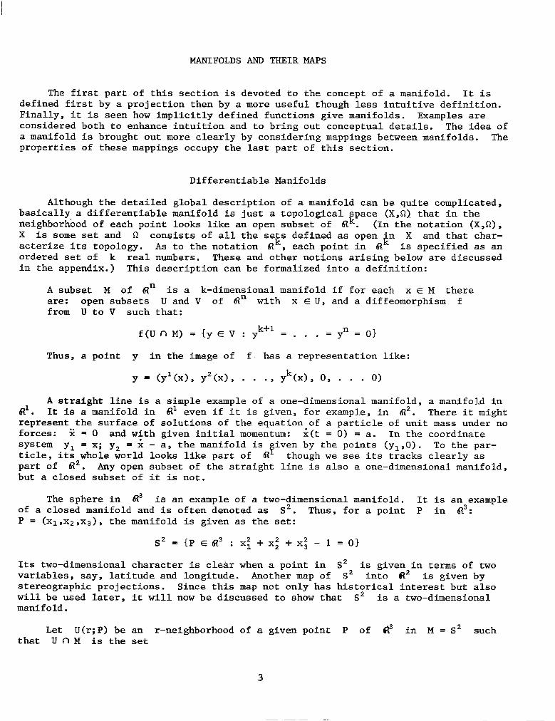


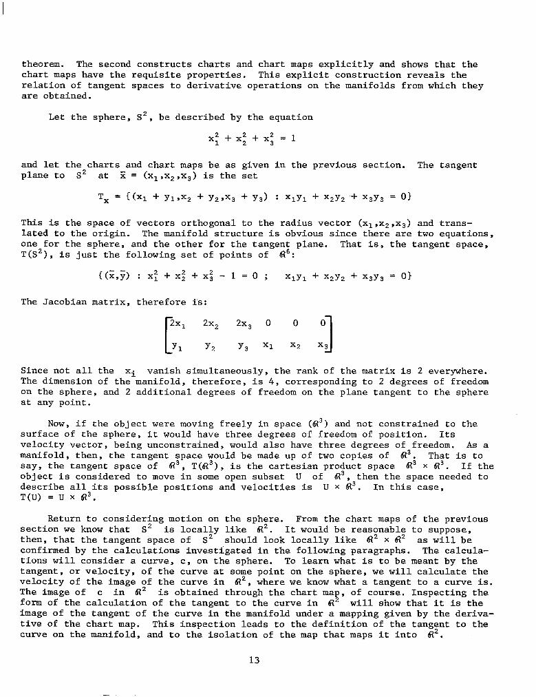


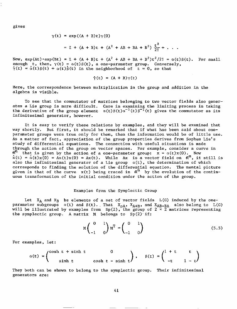


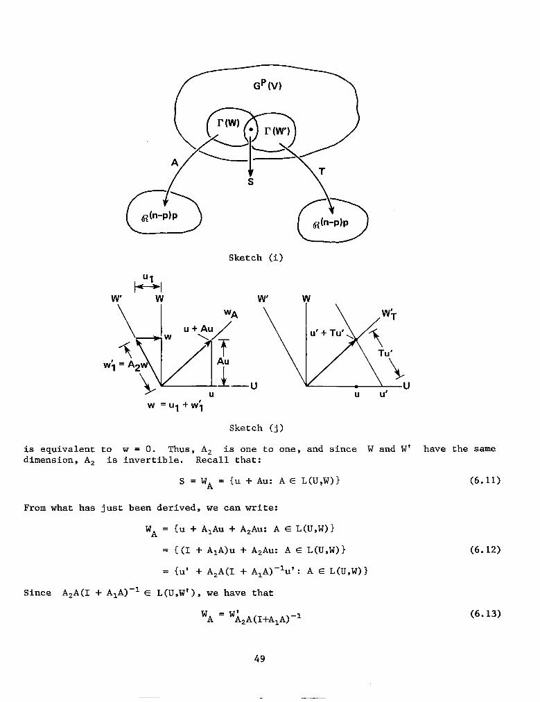


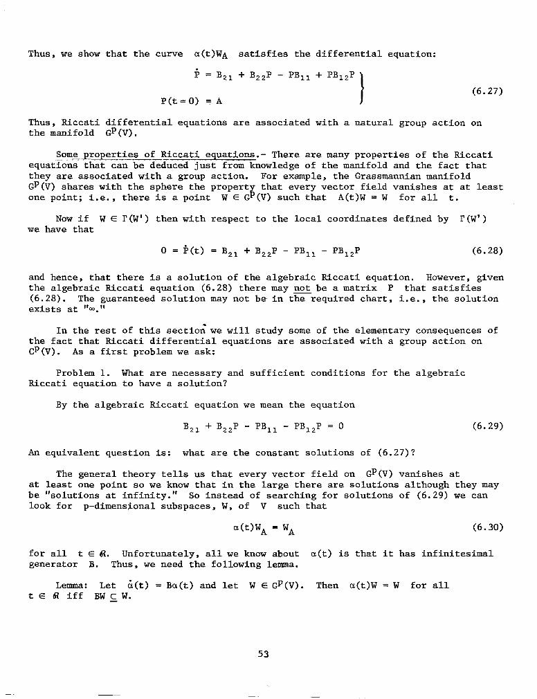

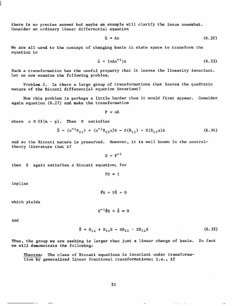


![Www.feedurbrain.com-James Doolin - How to Change Your Identity and Erase Bad Credit [eBook (PDF)]](https://static.documents.pub/doc/80x56/55720bc3497959fc0b8c2eb7/wwwfeedurbraincom-james-doolin-how-to-change-your-identity-and-erase-bad-credit-ebook-pdf.jpg)


![arXiv:1412.7167v1 [cond-mat.mes-hall] 22 Dec 2014 · Refractometric sensing of Li salt with visible-light Si 3N 4 microdisk resonators C. Doolin,a) P. Doolin, B.C. Lewis, and J.P.](https://static.documents.pub/doc/80x56/5e19814647eb1363c2367c1b/arxiv14127167v1-cond-matmes-hall-22-dec-2014-refractometric-sensing-of-li-salt.jpg)


