+ All Categories
Home > Documents > RReesseeaarrcchh RReeppoorrtt

RReesseeaarrcchh RReeppoorrtt

Date post: 06-Apr-2022
Category:
Upload: others
View: 3 times
Download: 0 times
Share this document with a friend
23
R R e e s s e e a a r r c c h h R R e e p p o o r r t t Department of Statistics No. 2013:2 A Comparison of Seasonal Adjustment Methods: Dynamic Linear Models versus TRAMO/SEATS Can Tongur Department of Statistics, Stockholm University, SE-106 91 Stockholm, Sweden Research Report Department of Statistics No. 2013:2 A Comparison of Seasonal Adjustment Methods: Dynamic Linear Models versus TRAMO/SEATS Can Tongur +++++++++++++++
Transcript

RReesseeaarrcchh RReeppoorrtt Department of Statistics

No. 2013:2

A Comparison of Seasonal Adjustment Methods: Dynamic Linear Models versus TRAMO/SEATS

Can Tongur

Department of Statistics, Stockholm University, SE-106 91 Stockholm, Sweden

Research Report

Department of Statistics

No. 2013:2

A Comparison of Seasonal

Adjustment Methods:

Dynamic Linear Models versus

TRAMO/SEATS

Can Tongur

+++++++++++++++

1

1

A Comparison of Seasonal Adjustment Methods:

Dynamic Linear Models versus TRAMO/SEATS

Can Tongur*

Stockholm University

&

Statistics Sweden

Summary

Seasonal adjustment can be done in the state space framework by Dynamic Linear Models. This

approach is compared with seasonal adjustment by TRAMO/SEATS. The comparison uses

simulated time series and real Swedish foreign trade data, the latter allowing a discussion on the

consistency issue in aggregation, i.e. direct versus indirect seasonal adjustment. We start by a

simple dynamic model and then increase the model structure using Gibbs sampling to identify

coefficients for the state evolution matrix. Our empirical study shows that the simpler state spate

approach exaggerates seasonal adjustment while the extended model with sampled coefficients

may offer a tool for seasonal adjustment. For simulated data, we find that TRAMO/SEATS is

better than the state space approach.

Key Words: Dynamic Linear Models, DLM, seasonal adjustment, consistency, foreign trade

* Statistics Sweden, BOX 24300, 10451 Stockholm, Sweden. Email: can.tongur (at) SCB.se

Acknowledgements: Daniel Thorburn, Stockholm University, spawned the idea behind this paper and gave guidance

and suggestions for its improvement. Lars-Erik Öller, Stockholm University, contributed with invaluable comments

that improved the understanding of the paper substantially. I am grateful for all their help in accomplishing this paper.

Disclaimer: As usual. All opinions in this paper are the ones of the author.

2

2

1. Introduction

In official statistics, seasonal adjustment is generally done either by TRAMO/SEATS or by X-12-

ARIMA. A drawback of these prevalent methods is their complexity since adjustments are based

on analysis in the frequency domain. Seasonal adjustment can alternatively be done by state space

modeling. Dynamic linear models (Harrison & Stevens, 1976) offer a Bayesian state space

approach that can be applied to seasonally patterned time series. Varieties of the state space

approach can be found in e.g. Durbin and Koopman (2001), Hyndman et al. (2008) and, for

ARIMA models, in Hamilton (1994).

In this paper, DLM is compared to TRAMO/SEATS. Comparisons are made on simulated series

and on Swedish foreign trade data, which opens for a comparison between direct and indirect

seasonal adjustment. Studies of direct and indirect adjustment of foreign trade data have been done

by Maravall (2006) and Hood & Findley (2001), based on TRAMO/SEATS and X-12-ARIMA,

respectively, and there seems not to be any comparison of DLM against these methods. In the

following, Section 2 presents the background necessary for operating DLM. In Section 3, the

problem of consistency is addressed and evaluation measures are presented. Practical shortcomings

of DLM are also mentioned. Section 4 contains a simulation study comparing the two methods. An

application on foreign trade is presented in Section 5, and the results are evaluated in Section 6.

Some conclusions end the paper in Section 7.

2. Dynamic Linear Models

2.1 Setting up the filter

The following notation comes from West & Harrison (1989). Normality is assumed throughout,

which, if necessary, may be replaced by assuming Student’s t distribution. Let tY be the univariate

time series observation and let tθ be an (n 1) vector of unobserved components. To assess the

latent model, we assume the following normality properties:

),(~)|( '

ttttt VNY θFθ (2.1a)

),(~)|( 11 ttttt N WθGθθ (2.1b)

The defining quadruple of the model },,,{ tttt V WGF contains (i) the coefficient vector tF of

dimension )1( n from the regression of tY on tθ , (ii) the )( nn state evolution matrix tG , (iii)

the observational error variance tV and (iv) the )( nn state innovation variance matrix tW . The

structures of the three elements tF , tG and tW are given in subsection 2.2. The distributions given

in expressions (2.1a, 2.1b) can be restated as a state space system:

Observation equation: tttt vY θF' , ),0N(~ tt V . (2.2a)

State equation: tttt ωθGθ 1 , ),(~ tt N W0ω . (2.2b)

The initial information set oD contains all information available at start and is updated by

additional observations on tY ; ),( 1 ttt DYD . When an observation is made, the posterior of the

unobserved state will be normally distributed with expected value m 1t and variance matrix C 1t :

3

3

a) Posteriors at t-1: ),(~)|( 1111 tttt ND Cmθ

To arrive at a) we first use the prior estimate of the state and its variance with the evolution

variance in expression (2.1b):

b) Prior at t: ),(~)|( 1 tttt ND Raθ .

By (2.1b), the expected value of the state vector is 1 tt Gma . The prior variance is subject to the

same forwarding and added the state innovation variance matrix tW : ttt WGGCR

'

1 .

The forecast distribution of tY based on all the information at t-1 follows:

c) One-step ahead forecast: ),(~)|( 1 tttt QfNDY , with ttf aF' and ttt VQ FRF

' .

When tY is observed, the posterior distribution in a) is obtained by applying the theory of

conditioning in multivariate normal distributions (Subsection 2.3) and by incorporating b) and c):

d) Posterior at t: ),(~)|( tttt ND Cmθ with tttt eAam and 'AQARC ttttt , where

1 ttt FQRA and ttt fYe .

The updating algorithm is started by assuming something (or nothing) about the state vector and its

variance:

e) Initial prior: ),N(~)( 00 Cmθ ot D

The unobserved system vector tθ contains all information about the system at a given time point t.

In our case tθ will collect the season, the trend and the trend evolution estimates, to be explained

in Subsection 2.2. The observation error t in expression (2.2a) contains not only the ordinary

measurement error but also one-period transient model effects, such as extreme weather impacts or

labor strikes.

tW is related to the system variance tC by tW = )( 11'

1

GGCt , where is a discount factor

)10( . The prior variance can be rewritten as 1'

11 '

GGCWGGCR tttt . The

discounting is a subjective choice of the magnitude of impacts of sudden fluctuations, and is

perhaps the most difficult choice in DLM. The proportional ( 11 ) should be kept low to avoid

model instability but may at the same time reflect the seasonal frequency in the data, c.f. monthly

or quarterly data. A large renders a small innovation variance with a (perhaps excessively)

smooth system vector, while a small renders a larger innovation variance, implying that the

system vector will account for more irregularity during a longer period. Rougier (2003) suggests a

in the interval [0.9, 0.99] with close attention to presumable bad choices.

The observational variance tV is generally not known and is assumed to have an inverse gamma

prior and equals the inverse precision 1 for the corresponding series. Then precision will

follow a Gamma prior with )2/,2/(~)|( 111 ttt dnGamD with 1tn being the number of

observations in the prior and with 1td the prior variance estimate. As observations accrue,

11 tt nn which adjusts the degrees of freedom for the Gamma distribution and

4

4

ttttt QeSdd /2

11 , and )2/,2/(~)|( ttt dnND . This updating may be carried on to the

update of the system variance and similarly, the covariance matrix is updated

])[/( 1 ttttttt SS QAARC' , ttt ndS / .

The forecast variance is updated with tS : 1

'

ttt SQ FRF , see c) on page 3.

2.2 Seasonal models

The two time-domain models used here are seasonal effects models and differ in the order of their

autoregressive component. The first order model (Model 1) is a local trend model, having a trend

and a trend evolution estimate. The second order model (Model 2) has an additional autoregressive

component. The trend in Model 1 is

)(

1,1

tttt (2.3a)

and in Model 2 it is

)(

1,12211

ttttt . (2.3b)

The evolution term is characterized by a random walk:

)(

2,1

ttt . (2.3c)

The seasonal effects are modeled as random walks:

)(

1,2,11,

s

ttt ss , (2.3d)

)(

2,3,12,

s

ttt ss ,

)(

,1,1,

s

pttpt ss .

Model 1 has state vector

)( ,2,1, ptttttt sss θ ' ,

and Model 2 has state vector

'

,2,1,1 )( pttttttt sss θ .

5

5

Model 1 Model 2

1

1111

'

1

'

1

100

010

011

p

pppp

p

p

tG

0

I000

0

0

(2.4) or

'

1

11111

'

1

'

1

'

121

1000

0100

0001

01

p

ppppp

p

p

p

tG

0

I0000

0

0

0

. (2.5)

tF projects the system vector on the observation; tF = ')0101( for Model 1 and tF =

')01001( for Model 2. As tF and tG are constant, the time subscripts can be

dropped. The seasonal components follow random walks and their development is due to the

structure of the covariance matrix tC , given below.

P is the seasonal dimension (e.g. p = 4 for quarterly data), which gives the number of parameters

n = p+2 or n = p+3, for the two models. The seasonal components must sum to zero in order to

eliminate the seasonal impacts over one full cycle (e.g. one year). To ensure this, a zero sum

constraint, 01

0|

p

i

i , is imposed on the initial prior of the seasonal block in 0θ . The covariance

matrix of tθ , ))'())((( θθθθ EEE tt = Cθ )|( DV will ensure that the zero-sum constraint is

always achieved for the seasonal components:

p

p

p

pp

p

p

ppp

p

Co

11

111

111

0

0

3

2

1

and

p

p

p

pp

p

p

ppp

pCo

11

111

111

00

00

0

3

2

1

41

Choosing 1 , 2 , 3 and 4 implies using different priors on component variances.

2.3 Revision analysis – smoothing

Standard methods like TRAMO/SEATS and X-12-ARIMA redo seasonal adjustment of previous

time points as new data become available. The Markov property of DLM implies that

backward estimation, i.e. a smoothing, is required to obtain revised estimates. The best possible

estimate of the previous seasonal vector, given the state at the current time point )|( 1 tt Dθ , is

obtained through the Kalman smoother. For any two vectors of normal variables X and Y , the

conditional expectation of X given Y takes the form

))( E(Y)(YVVE(X)Y|XE 1

YYXY , (2.6)

and the variance of X given Y is

6

6

YX

1

YYXYXX VVVVY)|V(X . (2.7)

The conditional distribution ),|()|( 111 ttttt YDD θθ is obtained by the joint distribution

( 11 |, ttt DYθ ). Recalling that 111 )|( ttt DE mθ and 1

''

1)|( tttt DYE GmFaF , the

covariance follows by right multiplication:

)|,(θ 1tt1t DYCov )|)ω(GθF,(θ 1ttt1t1t DνCov ' = )|GθF,(θ 1t1t1t DCov

' =

FGC'

1t = tY,θ 1t

V

. (2.8)

To reconsider step c) in subsection 2.1, the variance of the one-step ahead forecast is by definition

the covariance between tY and tY given the information at time point t-1, 1tD ;

)|,( 1ttt DYYCov = )|)(,)(( 11

'

1

'

ttttttt DCov ωGθFωGθF

= ttt V FWGGCF )( '

1

' = ttt QV FRF' . (2.9)

Then, the expected posterior, conditional on additional data, is

)(),|( 1'

1111 tttttttt fYQDYE

FGCmθ , (2.10)

and the variance is

1

1

1111 ''),|(

ttttttt QYDV GCFFGCCθ . (2.11)

3. Diagnostics of seasonally adjusted series

Evaluations of seasonal adjustments are often method-dependent, and there seems to be no

standard criteria. Common measures exist, of which some are used here. Additionally, seasonal

adjustment of times series that together constitute an aggregate, such as exports and imports,

yielding the trade balance, raises the issue of consistency, which will be addressed here.

3.1 Model diagnostics In the following, some evaluation measures are used for assessing the accuracy of seasonal

adjustment and the consistency between aggregations. The measures are either common to the

DLM and TRAMO/SEATS or merely adapted to the DLM because of computational limitations of

the TRAMO/SEATS output.

3.1.1 Mean squared error

For any estimated parameter , the mean squared error (MSE) is

T

t

t ET

MSE1

2

)(ˆ1 , (3.1)

7

7

which can be seen is scale-dependent but is still useful when comparing models on single series.

3.1.2 Model fit

Forecasting is not explicitly necessary for seasonal adjustment with DLM because of posterior

updating but model fit is still important and is here measured by (3.1) and the scale-free mean

absolute percentage error (MAPE) of forecasts tf :

T

pt t

tt

y

fy

pTMAPE

1

1. (3.2a)

This measure is undefined at 0ty so an alternative is to use a forecast error measure proposed

by Hyndman & Koehler (2008), also scale independent. This is named the mean absolute scaled

error (MASE) and targets comparing the model fit by relating it to an in-sample naïve forecast

error:

T

pt

tt

T

pt

tt fyyyMASE2

1

2

1 ||)||( (3.2b)

MASE is desired to be below unit value (<1), since unit value means that the forecast model is no

better than a naïve approach, i.e. the previous observation.

3.1.3 Residual seasonality in irregular components

A detrended and seasonally adjusted series should be purely white noise. Here, irregular

components are checked for autocorrelations. White noise autocorrelations should, under

normality, lie within pT /2 of zero on a 5% level (see Hamilton, 1994). This will be

visualized graphically. Autocorrelation coefficients are tested for significance by using the Ljung-

Box Q-statistic.

3.1.4 Revision

As new observations are made, seasonally adjusted next-to endpoint observations are revised. In

some sense, this revision is the conjectural misjudgment at the previous time point, given today’s

information. For DLM, the Markov property implies that the prior estimates are unchanged and

only the posterior distribution for the final data point is estimated. The mean absolute revision

error (MARE) of the system vector estimate can be computed as

MARE

J

j

T

jpt jtjt

jtjttjt

jpTJ 1 1 |

||

ˆ'

ˆ'ˆ'

)(

11100

θF

θFθF for j>0. (3.3a)

Equation (3.3a) should be interpreted as the revision in the entire model at any time point and the

concurrent season k: kjtjt s , . The smoothed state vector for period t-j, given t, is compared to

the benchmark from time t-j, i.e. the first estimate. Revision of each component can be analyzed

directly. The mean absolute revision error in the adjusted series can be defined as a simplification

of (3.3a):

8

8

J

j

T

jpt jtjt

jtjttjt

SA

SASA

jpTJDMARE

1 1 |

||

)(

11100 for j>0, (3.3b)

in which jtjtSA | is the seasonally adjusted series ( ),ktt sY for the coinciding season k at the first

occurring time point t-j while tjtSA | is the revised seasonally adjusted series , estimated at the later

time point t .

3.1.5 Roughness/smoothness

Dagum (1979) has proposed two different kinds of roughness measures for seasonally adjusted

data. One of the methods is applicable for all adjustment methods and the other being specific to

the X-11 methodology. The former is the difference ( ) between consecutive points of seasonally

adjusted data, is scale-dependent and is one of two components in the Hodrick-Prescott filter:

2

22

2

1 )() t

T

pt

T

pt

t SASASR

(3.4)

Note to (3.4): Since the DLM has an initial startup period of p observations, the first adjustment of interest is p+1 so R

should begin at p+2.

For simulated series, the benchmark will be the true roughness which is known while applied to

real series, this measure lacks objective evaluation criteria.

3.1.6 Signs of growth rates

Direction of the growth of a series is a core question when comparing seasonal adjustment

methods or aggregations. Direct and indirect seasonal adjustments should intuitively render the

same growth direction. The statistic of interest is thus the difference in sign of monthly and yearly

growth rates.

3.1.7 Discrepancy between aggregations

Direct and indirect seasonal adjustments are expected not to differ too much. Penalizing large

discrepancies between a direct estimation and the summarized estimation of k series is done by the

following distance measure:

T

pt

K

k

k

t

D

t SASAD1

1

2)( . (3.5)

4. Application to simulated data

A comparative study between DLM and TRAMO/SEATS should comprise mathematical

derivations of the methods, but this would be a tedious task, if even possible. Instead, we apply

these methods on a handful of simulated series with components predetermined. Five series, all

quarterly for parsimony, with different attributes are analyzed, see Figure 4.1. Each series is

simulated just once.

9

9

Figure 4.1 Illustration of the simulated series

Series 1 Series 2

Series 3 (in bold) and 4 Series 5

Seen in Figure 4.1, Series 2 has a level shift and in Series 3, the seasonal components are hard to

distinguish, i.e. weak seasonality (the growing line, in bold). Series 4 and 5 have a predictable

seasonal structure unlike Series 1 which has a perturbed seasonal pattern (see specifications in

Appendix A.2). The target of the simulations was to study how DLM and TRAMO/SEATS

captured the latent components. Since TRAMO has a head start in modeling the data generating

process (due to back-/forecasting), informative priors were obtained for DLM by two consecutive

runs. First, the filter was run with non-informative seasonal priors from t=1 to t=T. The posterior

seasonal estimates at the last time point (t=T) were then used as priors (after necessary reordering)

for the second run starting at t=1.

In Table 4.1, MSE of seasonal components, irregular component and the trend are given for

TRAMO/SEATS, DLM with and without informative priors based on a single run for each series.

Table 4.1 Mean squared error (MSE) of estimated components by TRAMO/SEATS and DLM Series Seasonal MSE Irregular MSE Trend MSE

TRAMO/

SEATS

DLM+ DLM++ TRAMO/

SEATS

DLM+ DLM++ TRAMO/

SEATS

DLM+ DLM++

1 96.4* 369.8 106.6 196.9* 658.7 382.1 793.7 624.7 605.8*

2 § 181.9 63 § 660.4 586.2 192.2* 874.6 1277

3 2.9 10.9 2.8 5.8* 25.3 18.8 15.6* 21.6 21.6

4 2.9* 117.2 3.7 10.4 76.3 8.6* 10.3* 27.7 13.9

5 2.5* 121.6 3.3 4* 87.1 7.3 10.8* 28.3 18.3

(+) Non-informative priors. (++) Informative priors. First p=4 observations are omitted in

MSE computations. (§) Measure not obtained accurately. * indicate the best measure.

TRAMO/SEATS seems to be generally more accurate than DLM in capturing the latent

components (10 cases of 15). With informative priors, DLM is better than TRAMO/SEATS in just

two cases, two cases are inconclusive and one case, seasonal MSE for Series 3, is a tie. This may

indicate that DLM is inadequately specified in this study, or perhaps assessing the problem in the

time domain is inferior to the frequency domain approach.

10

10

Table 4.2 MAPE and MASE of forecast errors and Ljung-Box Q.

Series MAPE MASE LB-Q

DLM + DLM ++ DLM+ DLM++ DLM + DLM ++ TRAMO/SEATS

1 0.06 0.04 0.56 0.41 61.0 * 33.8 9.6

2 0.08 0.08 0.47 0.42 85.8 * 111 * 19.7 *

3 0.07 0.06 0.67 0.58 28.5 33.6 11.0

4 0.08 0.04 0.39 0.18 62.1 * 24.6 13.8

5 0.02 0.01 0.16 0.07 230 * 21.2 13.8

Note: MAPE not possible to obtain from the standard output of TRAMO/SEATS. Critical value 36.41

for DLM, TRAMO/SEATS critical value is depending on model.

Seen in Table 4.2, informative priors are necessary when it comes to forecasting accuracy (MAPE,

MASE). The Ljung Box Q-statistic for squared residuals signals remaining seasonality in residuals

in all but one case of uninformative priors while using informative priors compares well with

TRAMO/SEATS.

5. Data and model specification

5.1 Data of the study

We use monthly Swedish trade data from January 1993 to July 2008, consisting of 187

observations, obtained from Statistics Sweden. The Intra-European trade is collected by the

statistical agency as a cut-off survey while the Extra-European trade is collected by the Swedish

Customs office as a census. Data of total exports and imports are known to be of high quality and

values reported here are in current prices, Million Swedish Kronor (SEK)

Figure 5.1 Exports and imports and Net trade. Original series, in Million SEK.

20,000

30,000

40,000

50,000

60,000

70,000

80,000

90,000

100,000

110,000

120,000

1993 1994 1995 1996 1997 1998 1999 2000 2001 2002 2003 2004 2005 2006 2007 2008 2009

EXPORTS IMPORTS

-2,000

0

2,000

4,000

6,000

8,000

10,000

12,000

14,000

16,000

18,000

20,000

22,000

1993 1994 1995 1996 1997 1998 1999 2000 2001 2002 2003 2004 2005 2006 2007 2008 2009

Net Trade

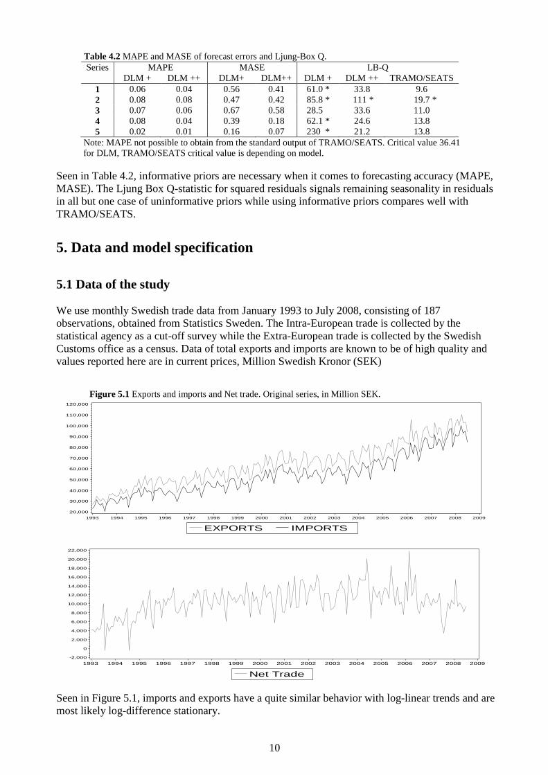
Seen in Figure 5.1, imports and exports have a quite similar behavior with log-linear trends and are

most likely log-difference stationary.

11

11

5.2 Specification of Model 1

The most stable models were found for in the neighborhood of 0.85, 0.9, 0.95 or 0.99, the last

being the default setting in BATS software (Bayesian Analysis of Time Series, see Pole, West and

Harrison, 1994). Smaller discount factors rendered either large or non-positive system error

covariance matrices, a situation also occurring in BATS.

The level prior was set to be the first observation (January 1993) and the trend variance prior set to

10 % of the squared mean of the series. Prior variances for the trend evolution, seasonal

components and observation variances 0V were set to one tenth (10%) of the prior trend variance.

This precaution of setting initial priors was due to the observed problems when specifying the

variance matrix – it was soon found that the definitional range of the variance matrix was quite

narrow, which also affected the choice of discount factors.

5.3 Specification of Model 2

Model 2 was specified similar to Model 1. The autoregressive parameters of the trend, which is a

latent variable, had to be estimated. The problem resembles parameter estimation in regression

analysis, also applicable to the state space setting. In order to estimate the trend persistency

coefficients 1 and 2 , a Markov Chain Monte Carlo procedure was used by applying a Gibbs

sampler for autoregression, see Lenk (2001). The latent component t in expression (2.3b) follows

by construction a normal distribution and assuming that regressors (components) have no

covariance (i.e. conditional maximum likelihood) will imply

),(~ 2

nt IN Aβ , (5.2)

where n is the number of observations until t , inclusive. E( t ) is given by Aβ where A by

definition is the data matrix obtained from the DLM recursion and β = ( 1 2 )’. The parameters

are β and 2 . Let the hypothetical likelihood of (5.2) be

)('()2(exp)()2(),|( 122/22/ AβαAβαAβα nnp (5.3)

This is a strong assumption, postulating (5.3) to be a real likelihood, while it only in fact exists by

construction. A is not obtained until the end of the recursion, consisting of all coherent trend

estimates. In that sense, this is a proper likelihood but obtained from a recursion.

The set of priors are:

)()(),( 22 ppp ββ (5.4)

),(~ 00 Vμβ N (5.5)

2,

2~ 002 sr

maInverseGam (5.6)

The posterior conditional distribution for β is

12

12

),(~),,|( 2

nnNp VμαAβ (5.7)

where the variance nV = 1

2

1

0 )'1

( AAVn

and the mean nμ = )1

(20

1

0 αA'μVVn

n

. 0V and

0μ are initial priors. The a posteriori conditional distribution for 2 is inverse Gamma

2,

2~),,|( 2 nn sr

IGp αAβ , (5.8)

where nrr on and RSSssn 0 (RSS = residual sum of squares). Having priors and

expressions for the conditional posteriors, and using Bayes’ rule to obtain the joint distribution

given the likelihood of data, a simplified Gibbs sampling can be used to get the parameters of

interest. The estimation of β is done by starting the Markov chain with an initial set of priors )0(β

and )0( , obtained from draws from expressions (5.5) and (5.6). The prior of )( jβ is plugged into

the DLM which is run through from t=1 to t=T. Residuals are obtained from the irregular

component, of which the sum of squared is taken as if it were a RSS from a linear regression. )( j is drawn from the inverse Gamma with shape parameter 2/ns and degrees of freedom

2/nr and used in the normal distribution from which the )( jβ are drawn. This procedure is repeated

1000 times (= chain length) after 200 burn-in observations and the average of the estimates of )(i

and )(i from overall 25 chains are used since the averages approximate a Monte Carlo integration

of the joint posterior.

5.4 TRAMO/SEATS specification

TRAMO/SEATS was operated in automatic mode here. The default model in the TRAMO is the

Airline model ARIMA(0,1,1)(0,1,1) against which other models are compared in estimation. No

calendar effects were used (RSA=3) in order to achieve comparability with DLM. Outliers were

treated by default, but not in DLM.

5.5 Software

The programming for this study considering DLM was done in Gauss ®. The algorithm was

verified by shadow programming in IML in SAS ®. TRAMO/SEATS ® was used in the Windows

version R12.6.

6. Estimation Results

Tables A.1 and A.2 show model estimates for four different discount factors. With respect to mean

squared error (MSE) of the irregular components and mean absolute percentage error (MAPE) of

forecasting, Model 1 with = 0.85 and Model 2 with = 0.9 were chosen for seasonal adjustment.

The coefficient sampling for Model 2 rendered practically same coefficients for all discount

factors.

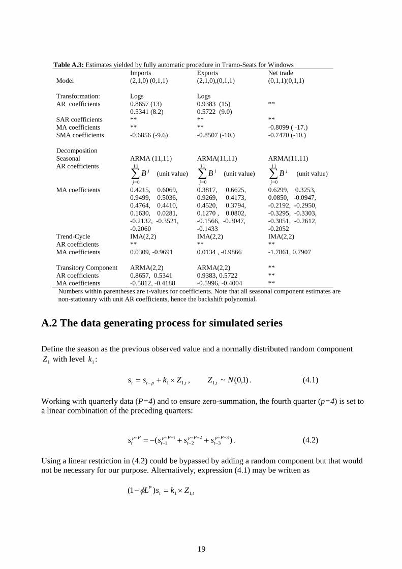
Estimates from TRAMO/SEATS are given in table A.3. For both exports and imports, an ARIMA

(2,1,0)(0,1,1) model was fit with correction for one and two outliers, respectively. The Airline

13

13

model was fit for the net trade series, with two additive outliers. Seasons were modeled as

ARMA(11,11) where each seasonal parameter was a function of the eleven preceding;

)...1( 112 BBBs with unit value for all AR-coefficients, similar to Maravall (2006). This

parametrization is discussed in Roberts & Harrison (1984). The trend-cycles were integrated

moving average, IMA(2,2). For both imports and exports, the TRAMO suggested an ARMA(2,2)

transitory component, meaning that the irregular components had a identifiable pattern for a

specific interval in the series.

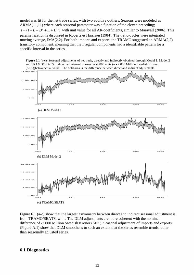
Figure 6.1 (a-c): Seasonal adjustments of net trade, directly and indirectly obtained through Model 1, Model 2

and TRAMO/SEATS. Indirect adjustment shown on -2 000 units (= - 2 000 Million Swedish Kronor

(SEK))below actual value. The bold area is the difference between direct and indirect adjustments.

(a) DLM Model 1

(b) DLM Model 2

(c) TRAMO/SEATS

Figure 6.1 (a-c) show that the largest asymmetry between direct and indirect seasonal adjustment is

from TRAMO/SEATS, while The DLM adjustments are more coherent with the nominal

difference of -2 000 Million Swedish Kronor (SEK). Seasonal adjustment of imports and exports

(Figure A.1) show that DLM smoothens to such an extent that the series resemble trends rather

than seasonally adjusted series.

6.1 Diagnostics

14

14

6.1.1. Mean Squared Error of forecasts

Seen in Table A.1, the lowest discount factor ( 85.0 ) for Model 1 yielded the smallest MSE for

all series so there was little gain from increasing the structure of DLM in Model 2 from a

forecasting point of view.

6.1.2 Model fit

In Tables A.1 and A.2, MAPE and MASE are given for both models. The two measures both

indicated that discount factors 0.85 and 0.9 were preferable for Model 1 and Model 2, respectively.

The MAPE behaved similarly in most cases for the two models but for the net trade, which is a

difficult and volatile series, Model 1 failed strongly with respect to MAPE.

6.1.3 Residual seasonality in irregular components

The irregular components are seen in Figure A.2 (a-f). The irregulars from Model 1 alternate with

smaller magnitude, closely related to the oversmoothing, while the irregulars from Model 2 are

larger and with a slightly more random appearance (scaling is different in figures). The

autocorrelation functions (ACF) are displayed in Figure A.3 (a-f) and the Ljung-Box Q statistic

(Table 6.1) indicate that residuals from Model 1 appear to be non-random with significant

autocorrelations while Model 2 has lower values than TRAMO/SEATS in two of three cases.

Table 6.1 Ljung-Box Q for autocorrelations of squared residuals.

Series Model 1 Model 2 TRAMO/SEATS

Exports 90.66 * 13.88 21.39

Imports 72.60 * 17.1 21.05

Net Trade 50.07 * 31.73 26.55

Critical value 36.41 (5 %).

6.1.4 Revisions of estimates

Revisions of the system vector (MARE) and the adjusted series (MARE-D) are small for both

specifications, Table A.1 and A.2, columns 5 and 6. This measure could not be tried for

TRAMO/SEATS, but empirical knowledge tells us that revisions can be large.

6.1.5 Roughness

Roughness ratios are given in Table 6.2, with TRAMO/SEATS as benchmark. The adjustments

from Model 2 were twice as rough as from Model 1, but both were markedly smaller than the

benchmark.

Table 6.2 Roughness ratios of DLM against TRAMO/SEATS based

on the roughness measure in expression (3.4)

Adjusted Series Ratio Model 1 /

TRAMO/SEATS

Ratio Model 2 /

TRAMO/SEATS

Imports 0.22 0.46

Exports 0.15 0.33

Net trade (direct) 0.10 0.23

Net trade (indirect) 0.09 0.21

15

15

6.1.6 Signs of growth rates

The direction of growth rates were controlled for when comparing the direct and indirect

approaches. Model 1 showed a consistent growth rate sign for both monthly and yearly rates, and

for Model 2, just 1 of 163 observations of the yearly rates differed. For TRAMO/SEATS, 5 of 163

yearly growth rates differed in sign between direct and indirect adjustments and 14 of 174 monthly

rates differed.

6.1.7 Discrepancy between aggregations

In Figure 6.1, the distances between adjustments are displayed. Numerically, it was 21 291 for

Model 1, 2 217 773 for Model 2 and 38 716 262 for TRAMO/SEATS, implying that for this

empirical case, the distance measure favored DLM. One obvious reason for the excellent non-

discrepancy in DLM may be the excessive smoothing that occurs in our cases.

6.2 Informative variance priors

Variance priors for Model 1 were obtained by considering the series during 12 months prior to start

in January 1993, i.e. entire 1992. Variance degrees of freedom was set to n=12. The trend was

assumed stable so the standard errors of the trend in exports and imports were set to 500 units

(each unit being 1 Million SEK) and 250 units for the net trade trend. The trend evolution is

considered more volatile, thus set to three times the trend standard error; 1 500 units for the two

trade series and 750 for the net trade series. Seasonal fluctuations can be a major part of the

volatility so standard errors for seasonal component were set to 5 000 units. Diagnostics are found

in Table 6.3.

Table 6.3 Model 1 Informative variance prior for imports, exports and

net trade. 85.0 . MSE and MASE of forecast MAPE. Revision

errors MARE and MARE-D. Series Delta MSE MAPE MASE MARE MARE-D

Imports 0.85 96 939 4.68 0.54 0.07 0.60

Exports 0.85 151 263 4.77 0.53 0.07 0.64

Net trade 0.85 55 683 19.58 0.74 0.30 2.51

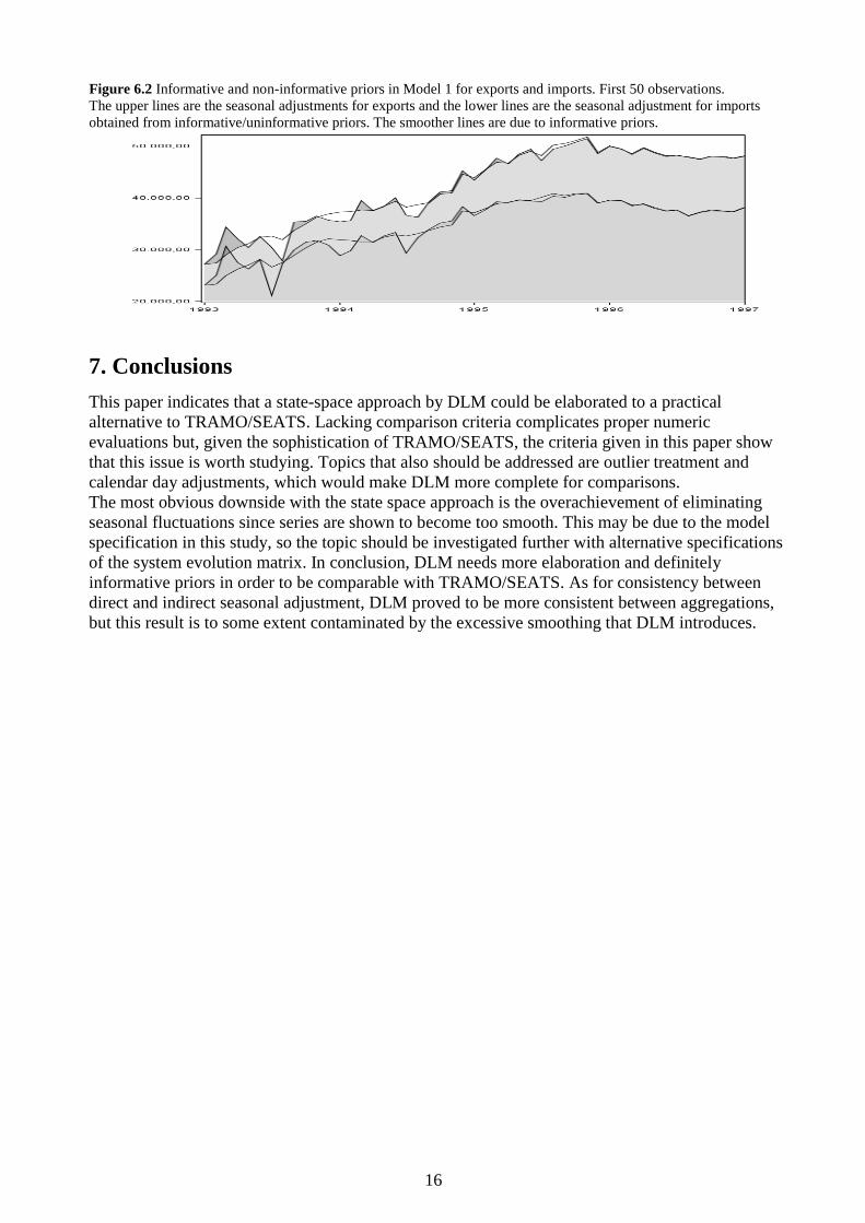
Seen in Figure 6.2, informative variance priors stabilize adjustments in the startup and

convergence between informative and uninformative priors is observed after some 40 observations

(i.e. 3-4 observations each season). The system variance showed a decrease of 20-25 % and overall

results indicate that back-casting, or two sequential runs (as with the simulated series), is necessary

for precision in the initial period.

16

16

Figure 6.2 Informative and non-informative priors in Model 1 for exports and imports. First 50 observations.

The upper lines are the seasonal adjustments for exports and the lower lines are the seasonal adjustment for imports

obtained from informative/uninformative priors. The smoother lines are due to informative priors.

7. Conclusions

This paper indicates that a state-space approach by DLM could be elaborated to a practical

alternative to TRAMO/SEATS. Lacking comparison criteria complicates proper numeric

evaluations but, given the sophistication of TRAMO/SEATS, the criteria given in this paper show

that this issue is worth studying. Topics that also should be addressed are outlier treatment and

calendar day adjustments, which would make DLM more complete for comparisons.

The most obvious downside with the state space approach is the overachievement of eliminating

seasonal fluctuations since series are shown to become too smooth. This may be due to the model

specification in this study, so the topic should be investigated further with alternative specifications

of the system evolution matrix. In conclusion, DLM needs more elaboration and definitely

informative priors in order to be comparable with TRAMO/SEATS. As for consistency between

direct and indirect seasonal adjustment, DLM proved to be more consistent between aggregations,

but this result is to some extent contaminated by the excessive smoothing that DLM introduces.

17

17

References

Dagum, E.B. (1979). On the Seasonal Adjustment of Economic Time Series Aggregates: A Case

Study of the Unemployment Rate, Counting the Labor Force. National Commission on

Employment and Unemployment Statistics, Appendix, 2, 317-344, Washington.

Cleveland, W.P. (2002). Estimated Variance of Seasonally Adjusted Series. A publication of the

Federal Reserve Board, Washington. Online resource available by October 1st, 2012 at:

http://www.federalreserve.gov/pubs/feds/2002/200215/200215pap.pdf

Hamilton, J. D. (1994). Time Series Analysis, Princeton University Press, Princeton New Jersey.

Harrison, J. P. & Stevens, C. F. (1976). Bayesian Forecasting, Journal of the Royal Statistical

Society. Series B (Methodological), Vol. 38, No. 3.

Hood, C. & Findley, D. F. (2001). Comparing Direct and Indirect Seasonal Adjustments of

Aggregate Series. ASA proceedings, October 2001.Online resource available by January 25th

,

2010 at: http://www.catherinechhood.net/choodasa2001.pdf

Hyndman, R.J., Koehler, A.B., Ord, J.K., Snyder, R.D. (2008). Forecasting with Exponential

Smoothing. The State Space Approach. Springer-Verlag Berlin Heidelberg.

Lenk, P. (2001). Bayesian Inference and Markov Chain Monte Carlo. Resource available online

by January 25th

, 2010 at: http://webuser.bus.umich.edu/plenk/Bam2%20Short.pdf

Maravall, A. (2006). An application of the TRAMO-SEATS automatic procedure; direct versus

indirect adjustment. Computational Statistics & Data Analysis 50, pp. 2167-2190.

Planas, C. & Campolongo, F. (2000). The Seasonal Adjustment of Contemporaneously

Aggreagated Series. Joint research centre of European Commission.

Pole, A., West, M. & Harrison, J. (1994). Applied Bayesian Forecasting and Time Series Analysis.

Chapman & Hall/CRC.

Roberts, S.A. & Harrison, P.J. (1984). Parsimonious modeling and forecasting of seasonal time

series. European Journal of Operational Research 16, pp. 365-377.

Rougier, J. (2003). Lecture Handouts on dynamic linear models. Online resource available by

January 25th

, 2010 at: http://maths.dur.ac.uk/stats/people/jcr/DLM

West, M. & Harrison J. (1989). Bayesian Forecasting and Dynamic Models. Springer-Verlag New

York Inc.

18

18

Appendix

A.1 Estimation results

Table A.1 Model 1 diagnostics for imports, exports and net trade. Discount

factor Delta, MSE of prior/forecast, MAPE and MASE of forecast, revision

errors MARE and MARE-D.

Series Delta MSE MAPE MASE MARE MARE-D

Imports 0.85 174 212 4.92 0.55 0.12 0.59

Exports 0.85 246 315 4.97 0.54 0.13 0.61

Net trade 0.85 88 183 26.66 0.74 0.43 2.27

Imports 0.90 934 175 5.29 0.59 0.21 0.43

Exports 0.90 1 345 568 5.16 0.56 0.21 0.43

Net trade 0.90 431 023 26.88 0.71 0.71 1.48

Imports 0.95 4 876 662 6.13 0.71 0.29 0.25

Exports 0.95 6 037 190 5.68 0.61 0.30 0.23

Net trade 0.95 1 617 775 27.93 0.71 0.88 0.74

Imports 0.99 22 497 135 7.62 0.92 0.35 0.08

Exports 0.99 21 595 272 6.90 0.74 0.34 0.07

Net trade 0.99 5 195 928 31.96 0.80 0.91 0.22

Table A.2 Model 2 diagnostics for imports, exports and net trade. Discount factor Delta,

estimated coefficient for trend, MSE of prior/forecast, MAPE and MASE of forecast,

revision errors MARE and MARE-D.

Series Delta Coefficients

)21(

MSE

MAP

E (%)

MASE MARE

(%)

MARE-D

(%)

Imports 0.85 0.782, 0.222 19 257 450 15.29 1.40

4.88 6.20

Exports 0.85 0.767, 0.234 388 670 5.35 0.58

0.15 0.68

Net trade 0.85 0.571, 0.400 92 568 10.26 0.74

0.41 2.22

Imports 0.90 0.782, 0.222 922 099 5.19 0.59

0.24 0.46

Exports 0.90 0.767, 0.234 1 349 663 5.13 0.56

0.24 0.46

Net trade 0.90 0.571, 0.400 454 264 9.51 0.72

0.62 1.42

Imports 0.95 0.782, 0.222 4 536 495 5.94 0.69

0.34 0.26

Exports 0.95 0.767, 0.234 5 908 991 5.61 0.61

0.33 0.25

Net trade 0.95 0.570, 0.401 1 711 259 9.41 0.70

0.72 0.71

Imports 0.99 0.782, 0.222 18 864 465 7.34 0.87

0.41 0.08

Exports 0.99 0.767, 0.234 20 435 229 6.79 0.73

0.40 0.08

Net trade 0.99 0.570, 0.401 4 495 395 10.94 0.73

0.76 0.20

Note that coefficients coincided for all settings of the discount factor.

19

19

Table A.3: Estimates yielded by fully automatic procedure in Tramo-Seats for Windows

Imports Exports Net trade

Model (2,1,0) (0,1,1) (2,1,0),(0,1,1) (0,1,1)(0,1,1)

Transformation: Logs Logs

AR coefficients 0.8657 (13)

0.5341 (8.2)

0.9383 (15)

0.5722 (9.0)

**

SAR coefficients ** ** **

MA coefficients ** ** -0.8099 ( -17.)

SMA coefficients -0.6856 (-9.6) -0.8507 (-10.) -0.7470 (-10.)

Decomposition

Seasonal ARMA (11,11) ARMA(11,11) ARMA(11,11)

AR coefficients

11

0j

jB (unit value)

11

0j

jB (unit value)

11

0j

jB (unit value)

MA coefficients 0.4215, 0.6069,

0.9499, 0.5036,

0.4764, 0.4410,

0.1630, 0.0281,

-0.2132, -0.3521,

-0.2060

0.3817, 0.6625,

0.9269, 0.4173,

0.4520, 0.3794,

0.1270 , 0.0802,

-0.1566, -0.3047,

-0.1433

0.6299, 0.3253,

0.0850, -0.0947,

-0.2192, -0.2950,

-0.3295, -0.3303,

-0.3051, -0.2612,

-0.2052

Trend-Cycle IMA(2,2) IMA(2,2) IMA(2,2)

AR coefficients ** ** **

MA coefficients 0.0309, -0.9691 0.0134 , -0.9866 -1.7861, 0.7907

Transitory Component ARMA(2,2) ARMA(2,2) **

AR coefficients 0.8657, 0.5341 0.9383, 0.5722 **

MA coefficients -0.5812, -0.4188 -0.5996, -0.4004 **

Numbers within parentheses are t-values for coefficients. Note that all seasonal component estimates are

non-stationary with unit AR coefficients, hence the backshift polynomial.

A.2 The data generating process for simulated series

Define the season as the previous observed value and a normally distributed random component

1Z with level 1k :

tptt Zkss ,11 , )1,0(~,1 NZ t . (4.1)

Working with quarterly data (P=4) and to ensure zero-summation, the fourth quarter (p=4) is set to

a linear combination of the preceding quarters:

)( 3

3

2

2

1

1

Pp

t

Pp

t

Pp

t

Pp

t ssss . (4.2)

Using a linear restriction in (4.2) could be bypassed by adding a random component but that would

not be necessary for our purpose. Alternatively, expression (4.1) may be written as

tt

P ZksL ,11)1(

20

20

where the autoregressive parameter 1 and PL is the seasonal lag operator Ptt

P yyL and

rather than using unit value for and making the correction in (4.2), zero summation could

alternatively be achieved by a more stringent specification of , see Cleveland (2002). The trend is

time-driven by a factor 2k and a multiple 3k of 1

0s to control the level and additionally incorporates

a uniformly distributed random component tUk 4 where )1,0(~ UniformU t :

tt UksktkT 4

1

032 . (4.3)

The irregular component is set to follow a normal distribution:

tt ZkI ,25 , )1,0(~,2 NZ t (4.4)

The simulated series are seasonally adjusted by Model 1 and by TRAMO/SEATS with automatic

model selection, presuming no calendar effects (parameter RSA=3).

Table A.4 Specifications of simulated series. Discount set to 0.9

Series T 1k 2k 3k 4k 5k Initial seasons

4

0

3

0

2

0

1

0 ,,, ssss

1 48 1k =1 2k = 2 3k =8 4k =100 5k =3 70,-30,-60,20

2 72 1k =2 2k =3 if t<37,

2k = -1 if t>36

3k =7 4k =70 if t<37,

4k = 50 if t>36

5k =3 50,-30, 10,-30

3 36 1k =3 2k =4 3k =3 4k =20 5k =3 10,-5,-8,3

4 36 1k =1 2k =3 3k =3 4k =10 5k =3 40,-13,-16,-11

5 84 1k =1 2k =log(t)*1/t 3k =6 4k =5 5k =3 60,-30,0,-30

Table A.4 gives the specifications of the simulated series. The first series has a slowly growing

level ( 22 k ) with large positive errors ( )1004 k and seasonal components with small noise

( 11 k ). The fifth series has a slowly decaying trend ( ttk /1*)log(2 , i.e. )(*)( xfxf ,

)log()( xxf ) with rather even and distinct seasonal components.

21

21

Figure A.1 (a-b): Seasonal adjustments of imports and exports. Estimation through Model 1 (on top), Model 2 on

minus 10 000 Million Swedish Kronor SEK of its actual value (in the middle) and TRAMO/SEATS on minus 20 000

Million Swedish Kronor SEK of its actual value (lowest line).

(a) Exports

0

10,000

20,000

30,000

40,000

50,000

60,000

70,000

80,000

90,000

100,000

110,000

1993 1994 1995 1996 1997 1998 1999 2000 2001 2002 2003 2004 2005 2006 2007 2008 2009

Model 1 Model 2 TRAMO/SEATS

(b) Imports

0

10,000

20,000

30,000

40,000

50,000

60,000

70,000

80,000

90,000

100,000

1993 1994 1995 1996 1997 1998 1999 2000 2001 2002 2003 2004 2005 2006 2007 2008 2009

Model 1 Model 2 TRAMO/SEATS

Figure A.2 (a-f): Irregular components of the two DLM models. Beware of scaling differences.

(a) Imports Model 1 (d) Imports Model 2

-4000

-3000

-2000

-1000

0

1000

2000

3000

4000

1 21 41 61 81 101 121 141 161 181

Irregular Component DLM(1)

Imports

-37000

-27000

-17000

-7000

3000

13000

23000

1 21 41 61 81 101 121 141 161 181

Irregular Component DLM (2)

Imports

(b) Exports Model 1 (e) Exports Model 2

-3000

-2000

-1000

0

1000

2000

3000

4000

1 21 41 61 81 101 121 141 161 181

Irregular Component DLM (1)

Exports

-40000

-30000

-20000

-10000

0

10000

20000

1 21 41 61 81 101 121 141 161 181

Irregular Component DLM (2)

Exports

22

22

(c) Net trade Model 1 (f) Net trade Model 2

-4000

-3000

-2000

-1000

0

1000

2000

3000

1 21 41 61 81 101 121 141 161 181

Irregular Component DLM (1)

Net trade

-4000

-3000

-2000

-1000

0

1000

2000

3000

4000

5000

6000

7000

1 21 41 61 81 101 121 141 161 181

Irregular Component DLM (2)

Net trade

Figure A.3 (a-f): Autocorrelations of irregular components for Model 1 and Model 2 with a 95 %

confidence bound.

(a) Imports Model 1 (d) Imports Model 2

-0,4

-0,3

-0,2

-0,1

0

0,1

0,2

0,3

0,4

Residual ACF Imports DLM (1)

-0,2

-0,15

-0,1

-0,05

0

0,05

0,1

0,15

0,2

Residual ACF of Imports DLM (2)

(b) Exports Model 1 (e) Exports Model 2

-0,4

-0,3

-0,2

-0,1

0

0,1

0,2

0,3

0,4

Residual ACF Exports DLM (1)

-0,25

-0,2

-0,15

-0,1

-0,05

0

0,05

0,1

0,15

0,2

Residual ACF Exports DLM (2)

(c) Net trade Model 1 (f) Net trade Model 2

-0,4

-0,3

-0,2

-0,1

0

0,1

0,2

0,3

0,4

Residual ACF Net trade DLM (1)

-0,2

-0,15

-0,1

-0,05

0

0,05

0,1

0,15

0,2

0,25

Residual ACF Net trade DLM (2)


Recommended