RRT*-Smart: Rapid convergence implementation of RRT* towards optimal solution Fahad Islam 1,2 , Jauwairia Nasir 1,2 , Usman Malik 1 , Yasar Ayaz 1 and Osman Hasan 2 1 Robotics & Intelligent Systems Engineering (RISE) Lab, Department of Robotics and Artificial Intelligence, School of Mechanical & Manufacturing Engg (SMME), National University of Sciences and Technology (NUST), H-12 Campus, Islamabad, Pakistan. 2 Department of Electrical Engineering, School of Electrical Engg & Computer Sciences (SEECS), National University of Sciences and Technology (NUST), H-12 Campus, Islamabad, Pakistan. { 08beefahad, 08beejnasir }@seecs.edu.pk, { usman, yasar }@smme.nust.edu.pk, [email protected]Abstract—Rapidly Exploring Random Tree (RRT) is one of the quickest and the most efficient obstacle free path finding algorithm. However, it cannot guarantee finding the most optimal path.. A recently proposed extension of RRT, known as Rapidly Exploring Random Tree Star (RRT*), claims to achieve convergence towards the optimal solution but has been proven to take an infinite time to do so and with a slow convergence rate. To overcome these limitations, we propose an extension of RRT*, called RRT*-Smart, which aims to accelerate its rate of convergence and to reach an optimum or near optimum solution at a much faster rate and at a reduced execution time. Our novel algorithm inculcates two new techniques in RRT*: these are path optimization and intelligent sampling. Simulation results presented in various obstacle cluttered environments confirm the efficiency of RRT*-Smart. I. INTRODUCTION The domain of Motion Planning involves finding a feasible trajectory that connects the starting point to the goal point while avoiding collision with the obstacles. The field of Motion Planning and Navigation has gained immense popularity and importance in the recent years due to the fact that current trends in robotics research for both industrial and domestic needs are focused towards intelligent automation. Since 1970s, many path planning algorithms including geometric algorithms, grid-based algorithms, potential field algorithms, neural networks, genetic algorithms and sampling based algorithms, have been proposed for various static and dynamic environments. Each of these algorithms has its own advantages and shortcomings in finding the most efficient path planning solution in terms of space and time complexity and path optimization [1-6]. Sampling based algorithms are among the latest and most popular path planning algorithms because they are less computationally complex and have the ability to find solutions without using explicit information about the obstacles in the configuration space as compared to other probabilistically complete algorithms. Instead, they rely on a collision checking module and build a roadmap of feasible trajectories made by connecting together a set of points sampled from the obstacle-free space. Rapidly Exploring Random Tree Star (RRT*) [7] is one of the recent sampling based algorithms. Its major advantage over other algorithms is that it finds an initial path very quickly and then later keeps on optimizing it as the number of samples increases. Thus, apart from probabilistic completeness it ensures asymptotic optimality [7] unlike its predecessor algorithm RRT [7][8]. Although RRT* claims to reach an optimal solution, it never reaches that optimality in finite time [7]. Also, the rate of convergence is slow. We address this problem by introducing RRT*-Smart which instead of employing purely random space exploration, performs an informed exploration of search space. It uses the first path found by RRT* as an intelligent guess to help in exploring the configuration space. Moreover, it uses intelligent sampling to give an optimum or near optimum path at a very fast rate of convergence and reduced execution time. The solution obtained by RRT*- Smart facilitates the robot to track the trajectory as it is straighter and with less way points. Thus, it gives a more efficient path planning solution as compared to RRT*. The remainder of the paper is organized as follows. In Section II, we discuss RRT*. RRT*-Smart is presented in Section III; while Sections IV and V cover Results and Performance Analysis, respectively. Section VI concludes the paper and highlights future research avenues. II. RRT* ALGORITHM As RRT*-Smart is an improved version of RRT*, so in this section we briefly introduce motion planning using the RRT* algorithm to build the background for understanding RRT*-Smart. RRT* is an incremental sampling based algorithm which finds an initial path very quickly and later optimizes the path as the execution takes place[7][9].
Transcript
RRT*-Smart: Rapid convergence implementation of
RRT* towards optimal solution
Fahad Islam1,2
, Jauwairia Nasir1,2
, Usman Malik1, Yasar Ayaz
1 and Osman Hasan
2
1Robotics & Intelligent Systems Engineering (RISE) Lab,
Department of Robotics and Artificial Intelligence,
School of Mechanical & Manufacturing Engg (SMME),
National University of Sciences and Technology (NUST),
H-12 Campus, Islamabad, Pakistan.
2Department of Electrical Engineering,
School of Electrical Engg & Computer Sciences (SEECS),
National University of Sciences and Technology (NUST),
Abstract—Rapidly Exploring Random Tree (RRT) is one of the
quickest and the most efficient obstacle free path finding
algorithm. However, it cannot guarantee finding the most
optimal path.. A recently proposed extension of RRT, known as
Rapidly Exploring Random Tree Star (RRT*), claims to achieve
convergence towards the optimal solution but has been proven
to take an infinite time to do so and with a slow convergence
rate. To overcome these limitations, we propose an extension of
RRT*, called RRT*-Smart, which aims to accelerate its rate of
convergence and to reach an optimum or near optimum solution
at a much faster rate and at a reduced execution time. Our novel
algorithm inculcates two new techniques in RRT*: these are
path optimization and intelligent sampling. Simulation results
presented in various obstacle cluttered environments confirm
the efficiency of RRT*-Smart.
I. INTRODUCTION
The domain of Motion Planning involves finding a
feasible trajectory that connects the starting point to the goal
point while avoiding collision with the obstacles. The field of
Motion Planning and Navigation has gained immense
popularity and importance in the recent years due to the fact
that current trends in robotics research for both industrial and
domestic needs are focused towards intelligent automation. Since 1970s, many path planning algorithms including
geometric algorithms, grid-based algorithms, potential field algorithms, neural networks, genetic algorithms and sampling based algorithms, have been proposed for various static and dynamic environments. Each of these algorithms has its own advantages and shortcomings in finding the most efficient path planning solution in terms of space and time complexity and path optimization [1-6]. Sampling based algorithms are among the latest and most popular path planning algorithms because they are less computationally complex and have the ability to find solutions without using explicit information about the obstacles in the configuration space as compared to other probabilistically complete algorithms. Instead, they rely on a
collision checking module and build a roadmap of feasible trajectories made by connecting together a set of points sampled from the obstacle-free space. Rapidly Exploring Random Tree Star (RRT*) [7] is one of the recent sampling based algorithms. Its major advantage over other algorithms is that it finds an initial path very quickly and then later keeps on optimizing it as the number of samples increases. Thus, apart from probabilistic completeness it ensures asymptotic optimality [7] unlike its predecessor algorithm RRT [7][8].
Although RRT* claims to reach an optimal solution, it
never reaches that optimality in finite time [7]. Also, the rate
of convergence is slow. We address this problem by
introducing RRT*-Smart which instead of employing purely
random space exploration, performs an informed exploration
of search space. It uses the first path found by RRT* as an
intelligent guess to help in exploring the configuration space.
Moreover, it uses intelligent sampling to give an optimum or
near optimum path at a very fast rate of convergence and
reduced execution time. The solution obtained by RRT*-
Smart facilitates the robot to track the trajectory as it is
straighter and with less way points. Thus, it gives a more
efficient path planning solution as compared to RRT*. The
remainder of the paper is organized as follows. In Section II,
we discuss RRT*. RRT*-Smart is presented in Section III;
while Sections IV and V cover Results and Performance
Analysis, respectively. Section VI concludes the paper and
highlights future research avenues.
II. RRT* ALGORITHM
As RRT*-Smart is an improved version of RRT*, so in
this section we briefly introduce motion planning using the
RRT* algorithm to build the background for understanding
RRT*-Smart. RRT* is an incremental sampling based
algorithm which finds an initial path very quickly and later
optimizes the path as the execution takes place[7][9].
Let X define the configuration space in which Xobs is the
obstacle region, Xfree=X/Xobstacle is the obstacle-free region
and Xgoal is the goal region. RRT* works to find out an input
u: [0:T] ϵ U that yields a feasible path x(t) ϵ Xfree that starts
from x(0) = x-initial to x(T)= goal following the system
constraints. While finding this solution, RRT* maintains a
tree Ƭ= (V, E) of vertices V sampled from the obstacle-free
state space Xfree and edges E that connect these vertices
together. This algorithm makes use of a set of procedures
which should be explained here before going into the details
of RRT*-Smart.
Sampling: It randomly samples a state zrand ϵ Xfree from
the obstacle-free configuration space.
Distance: This function returns the cost of the path between
two states assuming the region between them is obstacle free.
The cost is in terms of Euclidean distance.
Nearest Neighbor: The function Nearest (Ƭ, zrand) returns
the nearest node from Ƭ=(V, E) in terms of the cost
determined by the distance function.
Steer: The function Steer (zrand, znearest) solves for a
control input u[0,T] that drives the system from x(0)=zrand to
x(T)=znearest along the path x: [0,T] → X giving znew at a
distance ∆q from znearest towards zrand where ∆q is the
incremental distance.
Collision Check: The function Obstaclefree(x) determines
whether a path x:[0,T] lies in the obstacle-free region Xfree
for all t=0 to t=T.
Near-by Vertices: The function Near(Ƭ, zrand, n) returns the
nearby neighboring nodes that lie in a ball of volume (β
(logn/n)) around zrand where β is a constant that depends on
the planner.
Insert node: The function Insertnode(zparent, znew, Ƭ) adds
a node znew to V in the tree Ƭ =(V, E) and connects it to an
already existing node zparent as its parent, and adds this edge
to E. A cost is assigned to znew which is equal to the cost of
its parent plus the Euclidean cost returned by the Distance
function between znew and its parent zparent. A pseudo code describing RRT* is shown in Algorithm1.
complex environmental modeling and explicit information
about obstacles [2]. Furthermore they may not reach a
solution in environments containing obstacles with complex
geometries (concave, polygonal, circular etc).
Once the initial path has been found, intelligent sampling
starts with a certain number of samples being directly
spawned (lines 4-5) in a ball of radius Rbeacons centered at
zbeacons. The reason why sampling is biased towards these
beacons is that these beacons give a clue regarding the
position of obstacle vertices (or periphery in case of circular
obstacles). Therefore, these beacons need to be surrounded by
maximum nodes to optimize the path at these turns. Hence,
optimality is reached at much lesser number of iterations as
compared to RRT* which reaches a close to optimal solution
only as the samples approach infinity.
As the algorithm iterates, each time a new RRT* path with
smaller cost as compared to the previous path is found, an
optimized path is calculated. The cost of this optimized
Fig. 1 Path Optimization based on Triangular Inequality.
Fig. 2 (a) First Path given by RRT* at n=650. (b) An optimized path (in blue) is shown after the Path
Optimization technique is applied on the path shown in (a).
(c) shows clustered samples as a result of biasing towards the beacons (in green) at n=2500
(d) shows the optimum path at n=4200
path is compared with the previous optimized path. If the cost
is shorter, new beacons zbeacons are generated and thus new
biasing points are formed. These newly formed beacons are
closer to the vertices. This process continues until the
required iterations are completed.
Though the obstacles are not being explicitly defined
keeping the beneficial property of sampling based algorithms
intact, yet by using intelligent guessing and biasing beacons,
the proposed algorithm finds a way to spawn the tree nearer
to the vertices which eventually leads us towards an optimal/
near optimal path x:[zinit,zgoal] →optimal X. This path also
has a very few number of samples which is shown in Section
V. Hence RRT*-Smart algorithm works to provide a much
more optimal solution at a faster rate of convergence and an
easier path for the mobile robots to follow in any kind of
environment as the number of waypoints are less.
Fig. 2 demonstrates the effectiveness and working of
RRT*-Smart algorithm. An initial path is found in (a) at
n=650. In (b), Path Optimization yields an optimized path
shown in blue. The green dots are the beacons that are formed
for this initial path. After n=2500, Clustered samples are
formed around the beacons as shown in (c). Finally after an
iterative process, an optimized path is found for this obstacle
scenario at n=4200.
The Space and Time complexity for RRT* are given by
O(n) and O(nlogn), respectively [7]. Mathematical analysis of
RRT*-Smart shows that the space and time complexity is the
same as that of RRT* but the value of n is significantly
reduced in case of RRT*-Smart. Thus, O(n) and O(nlogn) for
RRT*Smart yields much better performance. However, as
the performance improves and the biasing ratio increases, the
randomness in the exploration of the tree decreases as a
number of nodes are now used to optimize the path in a
particular region. Therefore, there is a tradeoff between
intelligent sampling and space exploration rate.
IV. RESULTS
In this section, we show the optimized results for RRT*-
Smart in three environments with different obstacle scenarios.
The red box represents the goal region while the trajectory is
shown by a black line. It provides an optimal/ near optimal
solution in the circular, local minima and cluttered
environment. It can be observed that the path optimization
and intelligent sampling techniques that this algorithm
employs to provide a feasible path planning trajectory is
independent of the obstacle shape as highlighted in the
previous section.
V. PERFORMANCE COMPARISON
Here we present an experimental performance comparison
between RRT*-Smart and RRT* by analyzing their
performance from various perspectives. First we make use of
the results of the two algorithms in Fig. 4 to illustrate their
comparative differences.
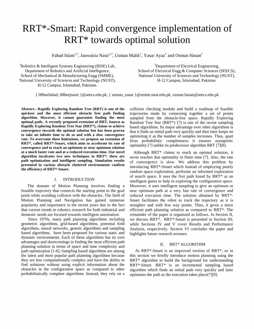
We see in Fig. 4(d) that RRT*-Smart uses the RRT* path
with a cost of 630.18 at iteration number n =800 shown in
Fig. 4(a) and finds a more optimal path with a cost of 584.02
at equal number of iterations using the Path Optimization
technique. With Intelligent Sampling and further path
optimization, the cost in Fig. 4(e) has further reduced to
557.478 at n=1200 while RRT* converging with its original
rate manages to reach a cost of 624.95 at the same number of
n in Fig. 4(b). Finally, RRT*- Smart gives an optimal/ near
optimal solution at n=4200 with a cost of 540.12 as shown in
Fig. 4(f). At the same number of iterations, RRT* converges
to a path with a cost of 574.009 in Fig. 4(c). The efficiency in
terms of path cost is evident from this comparison.
Next, we present a statistical comparison between the two
algorithms using graphical results for the experiment shown
in Fig. 4. In Fig. 5 the convergence pattern of the costs of
RRT* and RRT*-Smart is shown. It can be seen that RRT*-
Smart not only has a much faster rate of convergence but also
approaches the optimum cost after finite iterations whereas
RRT* is still in the process of reaching an optimal solution
with relatively slower rate of convergence.
Fig.3. RRT*-Smart in different obstacle Environments
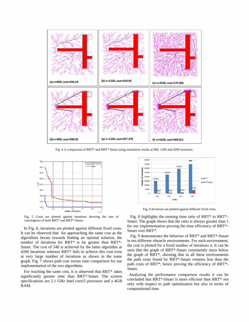
In Fig. 6, iterations are plotted against different fixed costs.
It can be observed that for approaching the same cost as the
algorithms iterate towards finding an optimal solution, the
number of iterations for RRT* is far greater than RRT*-
Smart. The cost of 540 is achieved by the latter algorithm at
4200 iterations whereas RRT* fails to achieve this cost even
at very large number of iterations as shown in the same
graph. Fig. 7 shows path cost versus time comparison for our
implementation of the two algorithms.
For reaching the same cost, it is observed that RRT* takes
significantly greater time than RRT*-Smart. The system
specifications are 2.1 GHz Intel corei3 processor and a 4GB
RAM.
Fig. 8 highlights the running time ratio of RRT* to RRT*-
Smart. The graph shows that the ratio is always greater than 1
for our implementation proving the time efficiency of RRT*-
Smart over RRT*.
Fig. 9 demonstrates the behavior of RRT* and RRT*-Smart
in ten different obstacle environments. For each environment,
the cost is plotted for a fixed number of iterations n. It can be
seen that the graph of RRT*-Smart consistently stays below
the graph of RRT*, showing that in all these environments
the path costs found by RRT*-Smart remains less than the
path costs of RRT*, hence proving the efficiency of RRT*-
Smart.
Analyzing the performance comparison results it can be
concluded that RRT*-Smart is more efficient than RRT* not
only with respect to path optimization but also in terms of
computational time.
Fig. 6 Iterations are plotted against different fixed costs.
Fig. 5 Costs are plotted against iterations showing the rate of
convergence of both RRT* and RRT*-Smart.
Fig. 4 A comparison of RRT* and RRT*-Smart using simulation results at 800, 1200 and 4200 iterations.
VI. CONCLUSION
Incremental sampling based algorithms have been widely in
use because of their advantages over other motion planners.
RRT* unlike RRT is asymptotically optimal apart from being
probabilistically complete. But the rate of convergence to this
close-to optimal solution is slow.
This paper presents a rapid convergence implementation of
RRT* known as RRT*-Smart which helps approaching an
optimal/ near optimal solution by introducing Intelligent
Sampling and Path Optimization techniques. Simulation
results have demonstrated that RRT*-Smart converges to
relatively optimal solutions at very few iterations and at an
accelerated rate. Performance comparison proved the
efficiency of RRT*-Smart with respect to both time and cost.
We expect to provide hardware results on Pioneer 3AT
Mobile Robotic platform in the near future and then precede
this work to dynamic environments.
REFERENCES
[1] M. Kanehara, S. Kagami, J.J. Kuffner, S. Thompson, H. Mizoguhi, "Path shortening and smoothing of grid-based path planning with consideration of obstacles," IEEE International Conference on Systems, Man and Cybernetics, 2007 (ISIC) , pp.991-996, 7-10 Oct. 2007.
[2] I. Petrovic and M. Brezak, “A visibility graph based method for path planning in dynamic environments”, in proceedings of 34th International Convention on Information and Commuincation Technology, Electronics and Microelectronics (MIPRO), pp.711-716,2011.
[3] N.H. Sleumer, N. Tschichold-Grman, “Exact cell decomposition of arrangements used for path planning in robotics” Technical report. Switzerland: Institute of Theoretical Computer Science Swiss Federal Institute of Technology Zurich; 1999.
[4] Y.K.Hwang, N. Ahuja , "A potential field approach to path planning," IEEE Transactions on Robotics and Automation,, vol.8, no. 1, pp.23-32, Feb 1992.
[5] A. Ghorbani, S, Shiry, and A. Nodehi,”Using Genetic Algorithm for a Mobile Robot Path Planning”, Proceedings of the 2009 International Conference on Future Computer and Communication ICFCC '09.
[6] S.X. Yang, C. Luo , "A neural network approach to complete coverage path planning," IEEE Transactions on Systems, Man, and Cybernetics, Part B: Cybernetics, vol. 34, no. 1, pp. 718- 724, Feb. 2004.
[7] S. Keraman and E. Farazolli, “Sampling-based Algorithms for Optimal Motion Planning” , International Jouranl of Robotics Research,2010.
[8] S. M. Lavalle and J.J. Kuffner, “Rapidly Exploring Random Trees: Progress and Prospects”, In Proceedings Workshop on the Algorithmic Foundations of Robotics, 2000.
[9] S. Karaman, Matthew R. Walter, A. Parez, E. Farazolli and S. Teller,”Anytime Motion Planning using the RRT”, in proceedings of International Conference on Robotic and Automation, pp. 1478-1483, 2011.
[10] M. Zucker, J. Kuffner and M. Branicky, “Multipartite RRTs for Rapid Replanning in Dynamic Environments”, in Proc. Of Internation Conference on Robotics and Automation, pp. 1603-160, 2007.
[11] DAB de Oliveira Vaz, Roberto S. Inoue and V. Grassi Jr, “Kinodynamic Motion Planning of a Skid-Steering Mobile RobotUsing RRTs”, in proceedings of Symposium on Artificial Intelligence,2010.
[12] A. Parez, S. Karaman, A. Shkolnik, E. Farazolli, Seth Teller and Matthew R. Walter “Asymptotically-optimal path planning for manipulation usin incremental sampling based algorithms”, in proceedings of International Conference on Intelligent Robots and Systems , pp. 4307-4313, 2011.
[13] Bialkowski, Karaman, and Frazzoli, “Massively Parallelizing the RRT and the RRT*,” in Proceedings of the IEEE/RSJ International Conference on Intelligent Robots and Systems (IROS), 2011.
Fig. 8 Running Time Ratio of RRT* over RRT*-Smart is plotted against iterations. Bias ratio b is taken as 2 for RRT*-Smart.
Fig. 9 Costs of path in ten different environments for 2000 iterations.
Fig. 7 Time comparison against fixed costs. Bias ratio b is taken as 2