Page 1
RULE-BASED RESERVOIR
MODELING BY INTEGRATION OF
MULTIPLE INFORMATION
SOURCES: LEARNING TIME-
VARYING GEOLOGIC PROCESSES
A REPORT SUBMITTED TO THE DEPARTMENT OF ENERGY
RESOURCES ENGINEERING
OF STANFORD UNIVERSITY
IN PARTIAL FULFILLMENT OF THE REQUIREMENTS FOR THE
DEGREE OF MASTER OF SCIENCE
By
Yinan Wang
March 2015
Page 3
iii
I certify that I have read this report and that in my opinion it is fully
adequate, in scope and in quality, as partial fulfillment of the degree
of Master of Science in Petroleum Engineering.
__________________________________
Prof. Tapan Mukerji
(Principal Advisor)
Page 5
v
Abstract
Rule-based modeling methodology has been developed to improve the integration of
geologic information into geostatistical reservoir models. Quantifying modeling rules
significantly aid in building geologically accurate reservoir models and reproduce the
intrinsic complexity of subsurface conditions. Especially when field data and geological
knowledge are both limited the way we utilize the rules is important. To expand the
application of rule-based reservoir modeling in various field cases, we propose a
systematic methodology of creating rules from other information sources.
Physical geomorphic experiments and process-based models contain time series
information we need for a reservoir model. Incorporating these two information sources
facilitate the rule induction for rule-based modeling and therefore help capture the
underlying uncertainty. Two examples are demonstrated in our study. A reference class
from tank experiments is created for turbidite lobe system, while a realization of a
process-based model is used to mimic and simulate channel network patterns and their
behaviors on a delta plain.
In our study, we assume that if an experiment is comparable to field data at a certain
interpretation scale, then the sedimentary processes and associated structures are
informative and provide at least some information about the resulting sedimentary
features at the comparable scale. Ripley’s K-function is utilized to analyze and extract
spatial clustering information of lobe elements at a given scale from experimental strata.
We convert the K function to modeling rules, allowing us to integrate clustering patterns
of turbidite lobes into surface-based models. Surface-based models successfully produce
a clustered point behavior and a stratigraphic framework comparable to the chosen
physical tank experiment. These models can be used to better assess subsurface spatial
uncertainty under such a stochastic process framework constrained by experimental
information.
To facilitate the utilization of process-based models, an automated tool for extraction of
channel features is developed with adjustable parameters for the optimal result. Multi-
Scale Line Tracking Algorithm is embedded and shows robust and accurate extraction of
channel networks from Delft3D models. Space colonization algorithm is proposed to
capture the developmental processes of channel network and reproduce a network pattern.
It is able to integrate theoretical knowledge and simulate a network coupling with feature
extraction tool.. The overall methodology is able to efficiently simulate channel networks
and their progradation through time given information from one or more realizations of
process-based models.
Page 7
vii
Acknowledgments
First of all, I want to thank my advisor Professor Tapan Mukerji. I am deeply indebted to
Professor Mukerji for his insightful advice and endless support over the past few years.
Life is always full of new journeys. Before I arrived in Stanford for a Petroleum
Engineering degree, I had been possessed by the beauty of geology for years.
Consequently, for quite a long term at Stanford I always tried to look at engineers' world
from the perspective of geologists and was extremely confused with my value to the team.
Instead of shaping me into an efficient worker, Professor Mukerji encouraged me to be
who I am and gave me freedom to explore my interest. I am very fortunate and grateful to
have him as my advisor.
I also owe my thanks to Professor Jef Caers and Professor Tim McHargue. They have a
very profound impact on me by sharing their expertise and research passion. Every time
when I have a conversation with them, I feel I grow up gradually, not just on my
development as a researcher, but on a general way of thinking. The best resources and
assets at Stanford are professors who guide students. I have been moving forward to be a
better man by talking with them and learning from them. And sometimes I only think of
taking classes and doing research as approaches to get in touch with them.
I would also like to thank Dr. David Hoyal and Dr. Hongmei Li for their meticulous
guidance during my internship with ExxonMobil. Both of them are true caring mentors to
me in the company. Working with them was such a pleasant experience. In the meantime
I also received great help from my advisor Professor Kyle Straub at Tulane University
and Professor Douglas Edmonds at Indiana University. Our many discussions and
subsequent work together has enriched my thoughts and studies immensely. One of my
magical changes happened at Tulane. Without Prof. Straub, I have not come this far from
where I started from.
Finally, I would like to acknowledge the financial support from Stanford Center for
Reservoir Forecasting (SCRF). And thanks to all the colleagues in SCRF, especially my
mentor, Siyao Xu. He guided me into fundamental thinking as an engineer. I owe him a
special thank you.
Page 9
ix
Contents
Abstract ............................................................................................................................... v
Acknowledgments............................................................................................................. vii
Contents ............................................................................................................................. ix
List of Tables ..................................................................................................................... xi
List of Figures .................................................................................................................. xiii
1. Introduction ....................................................................................................................1
1.1. Geologic Contexts ................................................................................................. 3
1.1.1. Submarine turbidite fan system ..................................................................... 3
1.1.2. Deltaic channel network system .................................................................... 4
1.2. Rule-based Modeling ............................................................................................ 6
1.3. Geomorphic Experiments ................................................................................... 10
1.4. Process-based numerical modeling ..................................................................... 11
2.Rule-based Model Construction ....................................................................................15
2.1. Rules and Their Classification ............................................................................ 15
2.2. Discussion on Model Complexity ....................................................................... 18
2.3. Modeling A Typical Channel-lobe System......................................................... 19
2.3.1. Compensational Stacking............................................................................. 21
2.3.2. Clustered Stacking ....................................................................................... 24
2.4. Rasterizing Rule-based Models .......................................................................... 26
3. Modeling Turbidite Lobes with Experimental Data .....................................................29
3.1. Methodology Overview ...................................................................................... 28
3.2. Quantitative Metric ............................................................................................. 30
3.3. Analyzing Experimental Data ............................................................................. 32
3.4. Modeling Sub-resolution Lobes .......................................................................... 35
3.5. Discussion ........................................................................................................... 37
4. Feature Extraction of Process-based Models ................................................................40
4.1. Network Skeleton................................................................................................ 39
4.2. Pre-processing of Topography Images ............................................................... 41
4.2.1. Supervised and Unsupervised Segmentation Methods ................................ 42
4.2.2. Multi-scale Line Tracking Algorithm .......................................................... 43
4.2.3. Tracking channel networks .......................................................................... 44
4.3. Post-processing of Topography Images .............................................................. 48
4.4. Application to Satellite Images ........................................................................... 52
4.5. Evaluation and Optimization of Feature Extraction Tool ................................... 53
4.6. Statistical Similarity ............................................................................................ 56
Page 10
x
5. Modeling River Networks .............................................................................................61
5.1. Characterizing Networks .................................................................................... 59
5.1.1. Directed graph .............................................................................................. 59
5.1.2. Network growth ........................................................................................... 60
5.1.3. Spatial distribution of bifurcation points ..................................................... 62
5.1.4. Intensity Analysis of Spatial Point Patterns ................................................. 63
5.2. Simulating A Growing Network ......................................................................... 65
5.2.1. Space colonization algorithm ....................................................................... 65
5.2.2. Generation of open and closed network patterns ......................................... 68
5.2.3. Generation of multiple realizations .............................................................. 71
5.3. Surface-based Modeling ..................................................................................... 72
6. Conclusions and Future Work ......................................................................................78
6.1. Summary and Conclusions ................................................................................. 76
6.2. Recommendations for Future Work.................................................................... 77
Nomenclature .................................................................................................................... 79
References ......................................................................................................................... 80
Page 11
xi
List of Tables
Table 2-1: Summary of rules for rule-based modeling used in our work ......................... 18
Page 13
xiii
List of Figures
Figure 1-1: Major uncertainty variables impacting water flood performance. Focus of this
report is marked by red color. ............................................................................................. 2
Figure 1-2: Distributary Lobe System formed in a feeder canyon. After Bouma and Stone
(2000) .................................................................................................................................. 3
Figure 1-3: Demonstration of deltas with complex channel networks (Source: NASA) ... 5
Figure 1-4: Demonstration of general rule-based modeling approach ............................... 9
Figure 1-5: Overhead photo of TDB-10-1 and schematic diagram of Tulane Delta Basin
facility. .............................................................................................................................. 11
Figure 1-6: Experiment basin design and photograph taken approximately 15.0 hr into the
DB-03 experiment (After Straub, 2009). ......................................................................... 11
Figure 1-7: Demonstration of a Delft3D realization and its modeling approach. ............ 13
Figure 2-1: Demonstration of scale and scope in rule-based models ............................... 16
Figure 2-2: Demonstration of hierarchical framework imposed in the forward modeling.
........................................................................................................................................... 20
Figure 2-3: Demonstration of workflow to determine the position of parent events using
combined probability map ................................................................................................ 21
Figure 2-4: Representation of proximal channel trajectory based on cardinal spline. ...... 23
Figure 2-5: Demonstration of generating a single event using surface-based modeling .. 24
Figure 2-6: Demonstration of positioning offspring lobes based on CDF........................ 25
Figure 2-7: Depositional maps of one single flow event, a cluster and five clusters. ...... 27
Figure 2-8: Workflow to convert surfaces to volumetric data for flow simulation .......... 27
Figure 3-1: Demonstration of workflow for reservoir modeling using experimental data 29
Figure 3-2: Demonstration of lobe elements in TDB-10-1 ............................................... 30
Figure 3-3: Demonstration of tree structure showing hierarchy of multi-scale lobes. ..... 31
Figure 3-4: Demonstration of spatial points indicating center locations of preserved lobe
complexes. ........................................................................................................................ 31
Page 14
xiv
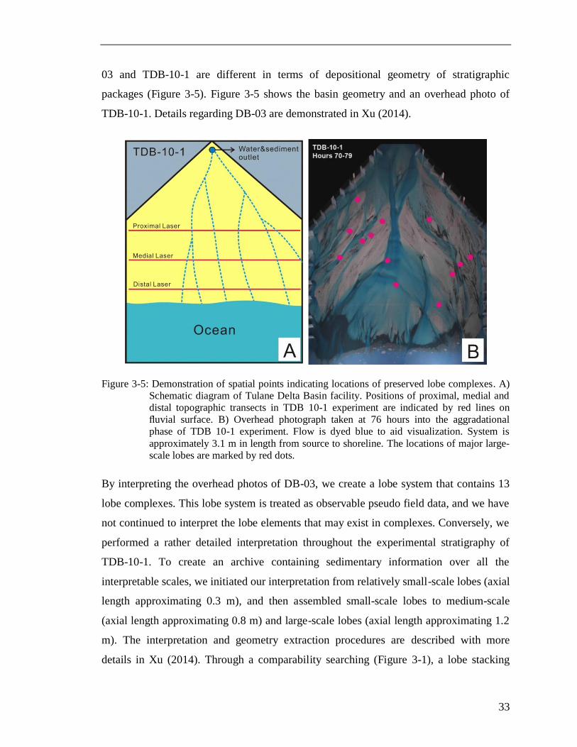
Figure 3-5: Demonstration of spatial points indicating locations of preserved lobe
complexes. ........................................................................................................................ 33
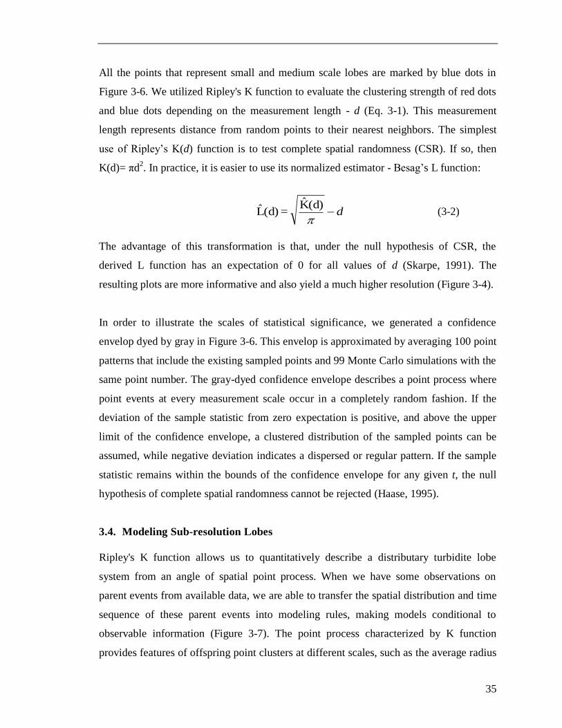
Figure 3-6: Demonstration of Ripley's K plots at three major interpretation scales. ........ 34
Figure 3-7: Model inputs and associated realization demonstration. ............................... 36
Figure 3-8: Comparison between K functions of inputs and modeling results Discussion.
........................................................................................................................................... 37
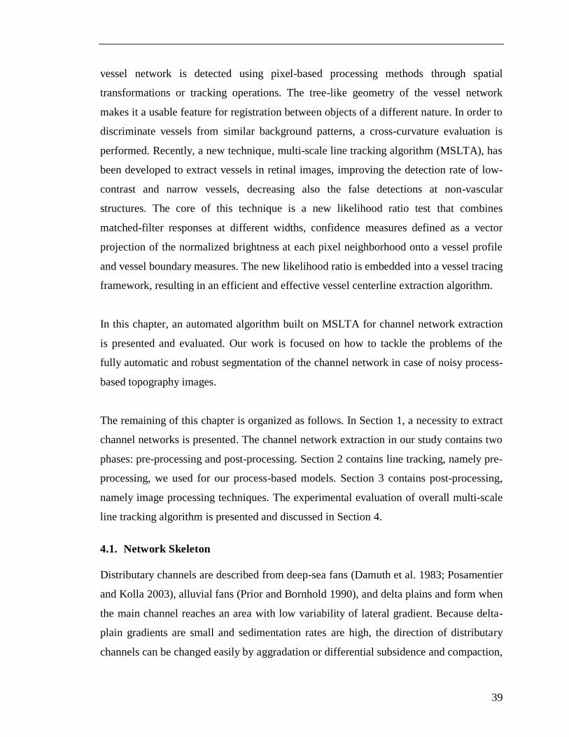
Figure 4-1: Satellite image of current Wax Lake Delta and its channel network skeleton
(After Hanegan, 2011). ..................................................................................................... 41
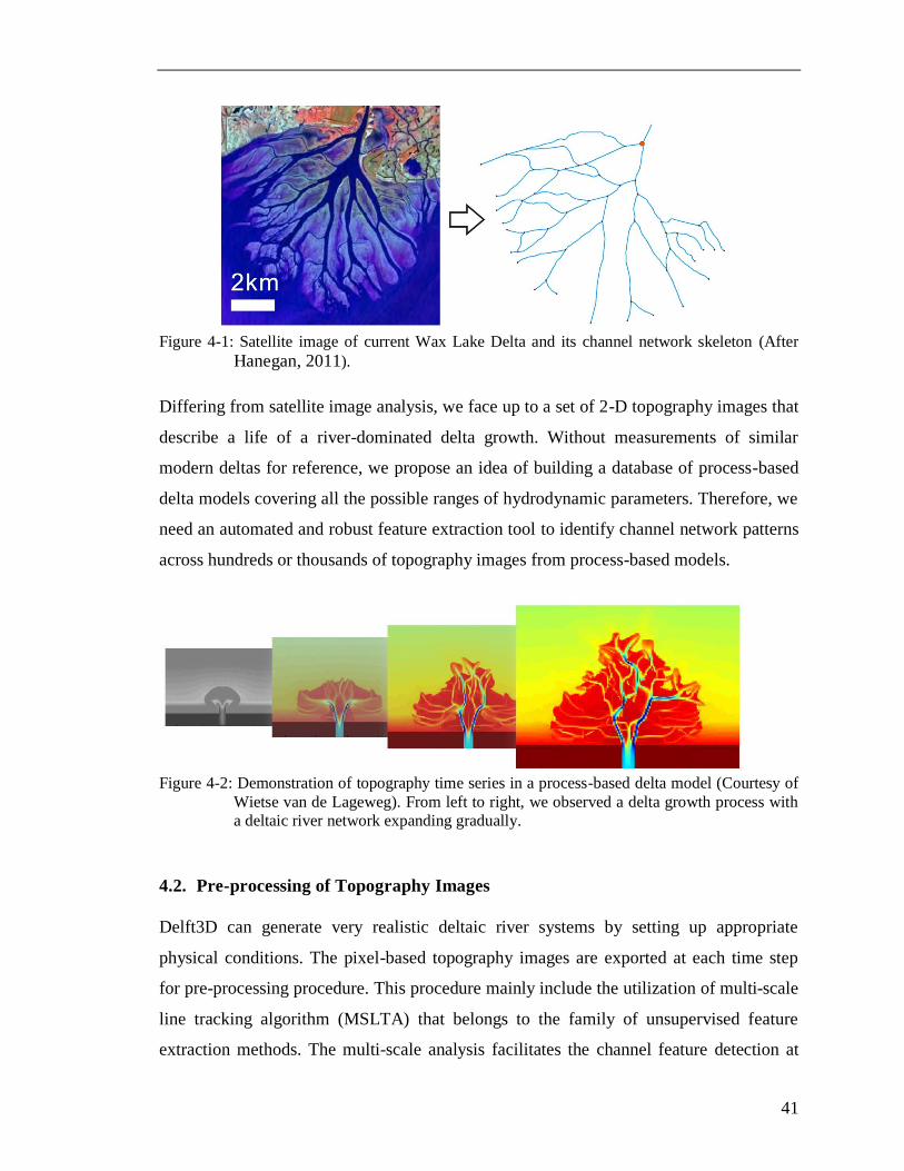
Figure 4-2: Demonstration of topography time series in a process-based delta model
(Courtesy of Wietse van de Lageweg). ............................................................................. 41
Figure 4-3: Flowchart of channel network extraction from topography images. ............. 44
Figure 4-4: Demonstration of a 2-D topography image in a time series generated by
Delft3D and its Cartesian grid. ......................................................................................... 45
Figure 4-5: Demonstration of curvature calculation. ........................................................ 46
Figure 4-6: Transformation of original topography into a confidence map and a binary
channel network. ............................................................................................................... 47
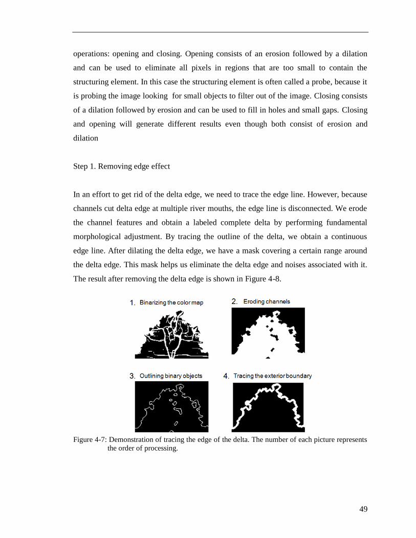
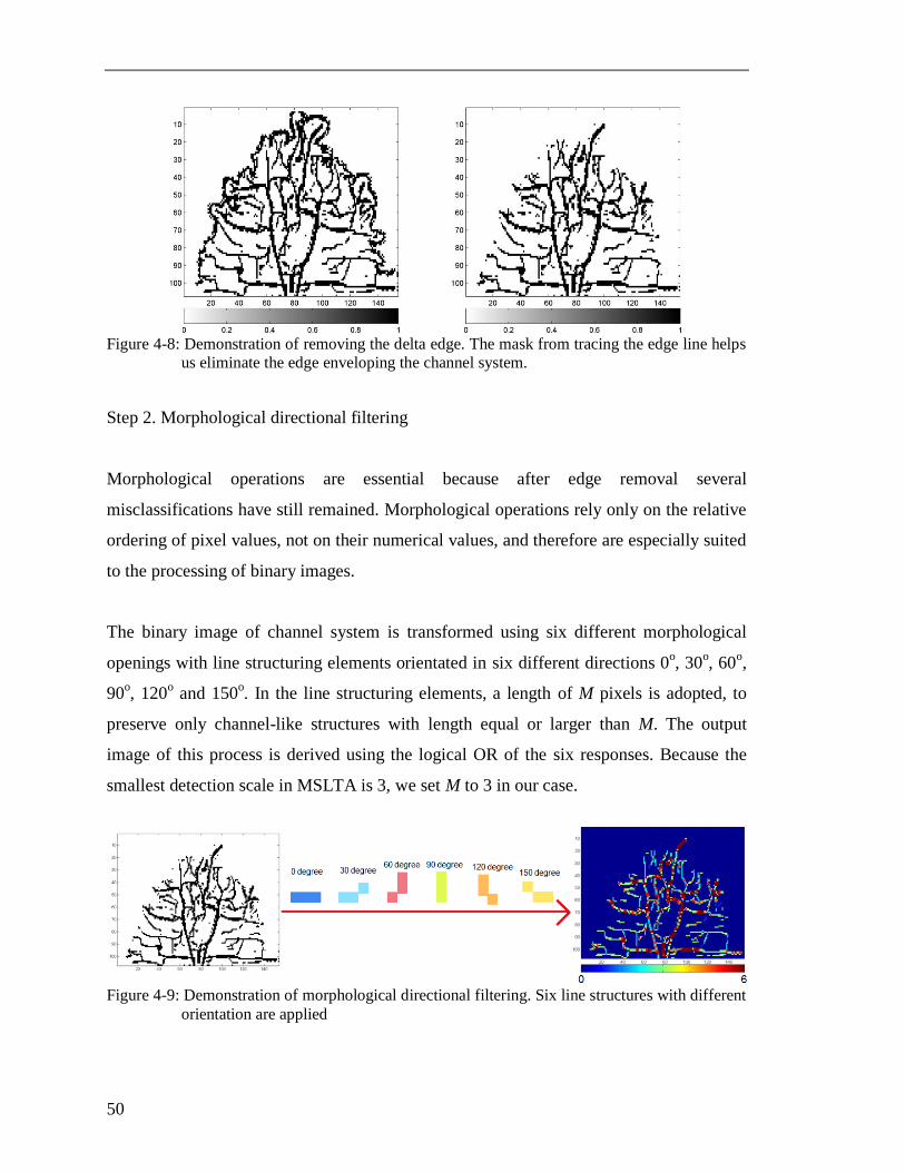
Figure 4-7: Demonstration of tracing the edge of the delta. The number of each picture
represents the order of processing.................................................................................... 49
Figure 4-8: Demonstration of removing the delta edge. ................................................... 50
Figure 4-9: Demonstration of morphological directional filtering. .................................. 50
Figure 4-10: Demonstration of morphological reconstruction. ........................................ 51
Figure 4-11: Demonstration of morphologically reconstructing the channel network. .... 51
Figure 4-11: Demonstration of confidence map and channel network obtained by
performing feature extraction from original Wax Lake Delta satellite image. ................. 52
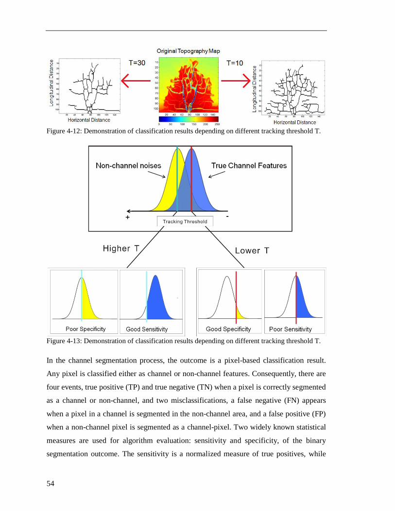
Figure 4-12: Demonstration of classification results depending on different tracking
threshold T. ....................................................................................................................... 54
Figure 4-13: Demonstration of classification results depending on different tracking
threshold T. ....................................................................................................................... 54
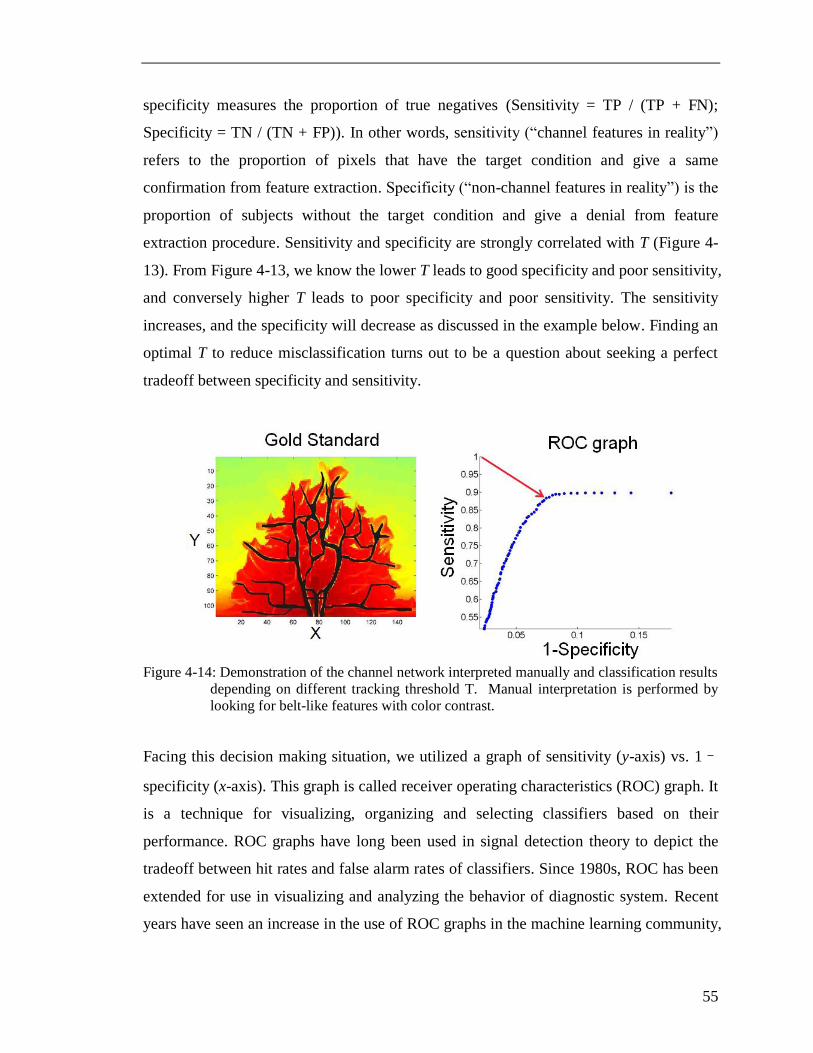
Figure 4-14: Demonstration of classification results depending on different tracking
threshold T. ....................................................................................................................... 55
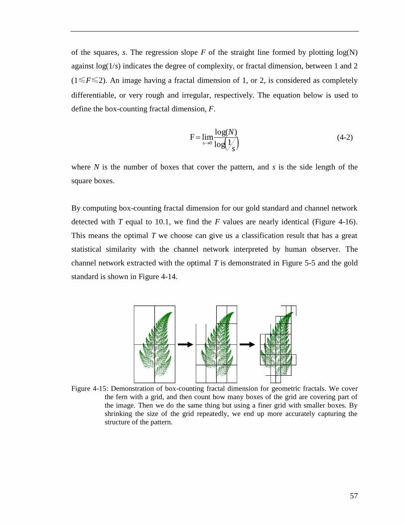
Figure 4-15: Demonstration of box-counting fractal dimension for geometric fractals. .. 57
Page 15
xv
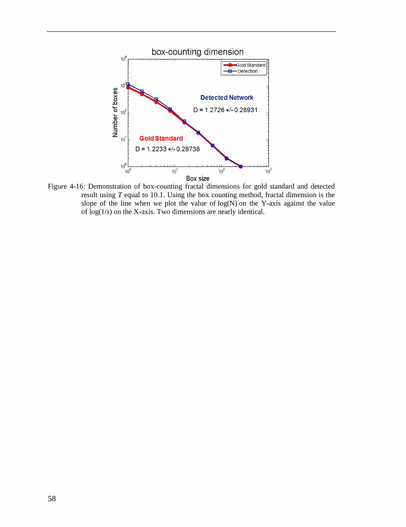
Figure 4-16: Demonstration of box-counting fractal dimensions for gold standard and
detected result using T equal to 10.1. ............................................................................... 58
Figure 5-1: Demonstration of a directed graph for a segment of channel network. ......... 60
Figure 5-2: Serial maps of Mossy delta, Saskatchewan, Canada (After Oosterlaan and
Meyers, 1995). .................................................................................................................. 61
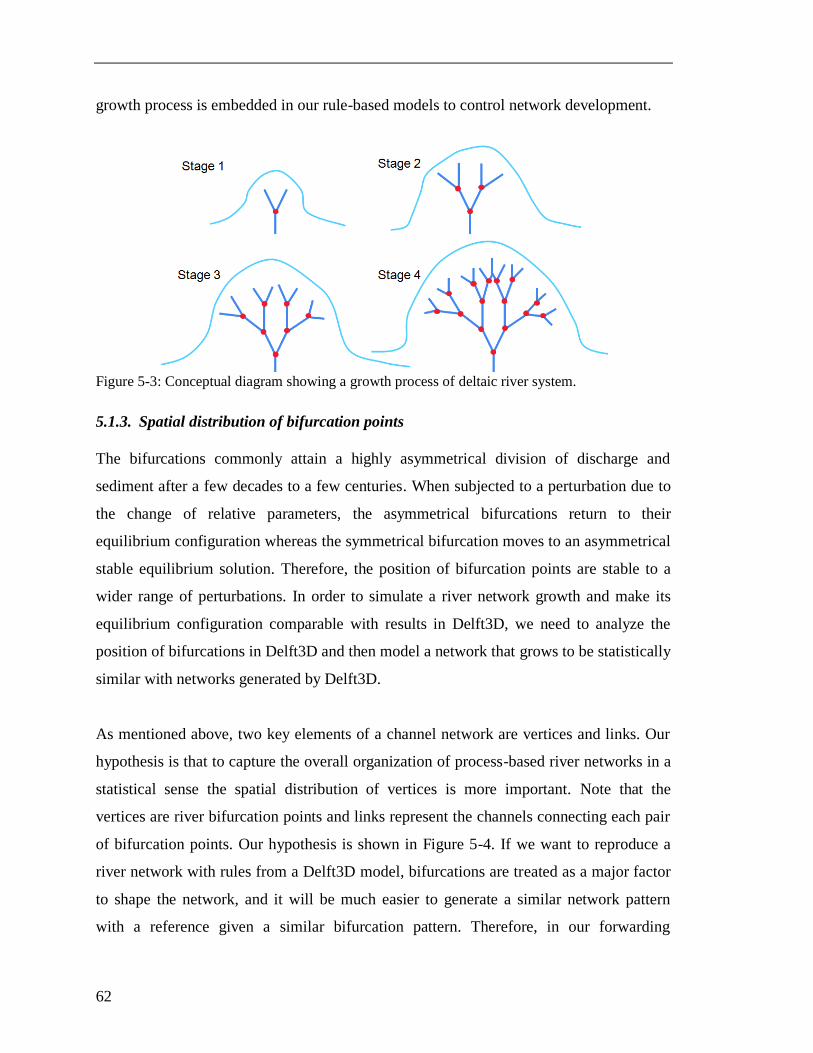
Figure 5-3: Conceptual diagram showing a growth process of deltaic river system. ....... 62
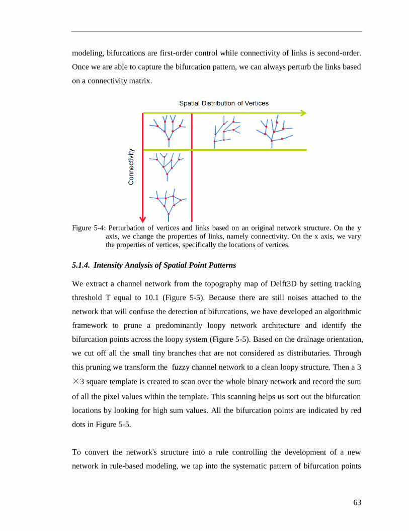
Figure 5-4: Perturbation of vertices and links based on an original network structure. ... 63
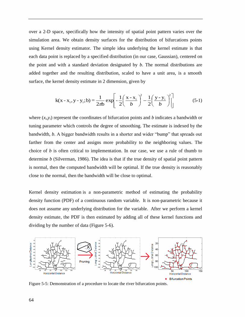
Figure 5-5: Demonstration of a procedure to locate the river bifurcation points. ............ 64
Figure 5-6: Kernel density estimate and PDF of bifurcation points on the river network.
........................................................................................................................................... 65
Figure 5-7: Illustration of channel network growth using space colonization algorithm . 67
Figure 5-8: Comparison between newly generated point pattern and original point pattern.
........................................................................................................................................... 69
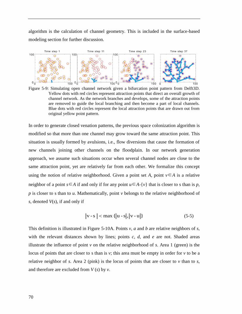
Figure 5-9: Simulating open channel network given a bifurcation point pattern from
Delft3D.. ........................................................................................................................... 70
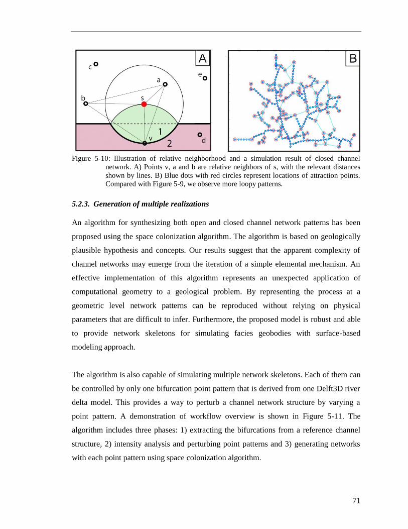
Figure 5-10: Illustration of relative neighborhood and a simulation result of closed
channel network. ............................................................................................................... 71
Figure 5-11: Illustration of generating multiple channel networks anchored to only
reference network.............................................................................................................. 72
Figure 5-12: Illustration of generating channel network skeleton and template boundaries
of deposits.. ....................................................................................................................... 73
Figure 5-13: Illustration of surface-based model based on network skeleton. ................. 74
Page 17
1
Chapter 1
1. Introduction
At early production stage of an oil or gas field, geologists often find that a hydrocarbon
accumulation consists of a number of fluid or pressure compartments. Different
compartments may contain different oil water contacts and fluids of different composition.
Dynamic surveillance data are very useful to help us detect the existing segments and
their positions. However, when we have production data, this assessment is too late to be
made in terms of retrieving the investment spent on an ongoing development plan. We
may have already overestimated the profitability of a field due to a misunderstanding of
reservoir compartmentalization. In extreme cases, reservoir compartmentalization might
even incur an abandonment of early fields. Therefore, we must perform compartment
assessment during the appraisal as early as possible given the situation that dynamic
production data are not available. A better understanding of in-situ compartments allows
us to accurately forecast the volume of reserves and hatch proper development strategies.
During appraisal, inadequate data in large part hinder the progress of compartment
evaluation. Limited numbers of wells may be the only data source for reservoir
characterization if seismic imaging is imperfect in mapping rock properties and
architecture. In addition, we may place too much emphasis on one aspect of the evidence
and then make further assumptions that bias data acquisition and interpretations.
Reservoir models are invoked to represent poorly known subsurface phenomena and
capture objective explanations to obtainable raw data. For risk mitigation and
development design, we must realistically assess reservoir uncertainty using reservoir
models as early as possible given the situation that only a few wells, 3D seismic data,
well testing and early production data are available at hand.
Page 18
2
Figure 1-1: Major uncertainty variables impacting water flood performance. Focus of this report
is marked by red color.
There are three key components - structures, depositional facies and petrophysical
properties, associated with a complete reservoir model (Figure 1-2). When facing an
unknown subsurface situation, we would incorporate as much information as possible in
reservoir models for better understanding about how much value will come out in terms
of reservoir performance. This report is focused on facies modeling. At the appraisal
stage, the types of depositional systems may be resolved, but the nature of facies
architectural elements and their interrelationship in the 3D space remains highly uncertain.
Reconstructing the depositional systems and resulted stratigraphy from a spatial and
temporal perspective is a key to assess this uncertainty. Thus, modeling hydrocarbon-
bearing reservoirs in a rule-based format yields a better appreciation of the roles played
by individual geological mechanisms in generating collective behavior. Linking
stratigraphic architecture to behavioral time series of a depositional system will produce
more informed strategies for intervention in the case of production forecasting and will
help us distill the principles that enabled sediments to evolve such versatile reservoir
systems in the first place.
In inducing rules to mimic geological processes, however, there is ample opportunity for
mistakes. In fact, it is not mainly the issue to reflect a real system by correctly translating
modeling rules and programming. First of all, for a specific depositional setting,
geological mechanisms are still obscure to us. Therefore, to create rules, we cannot rely
only on the use of heuristics by human experts. Secondly, integrating things we proclaim
to be correct into a computer model could lead to a bias. Generating a forecast for
reservoir performance is always an uncertain affair. Overwhelming artificial rules would
potentially restrict the understandings of realistic subsurface uncertainties and risks. To
Page 19
3
solve those problems mentioned above, I propose a rule induction approach that
integrates both empirical and theoretical knowledge from physical geomorphic
experiments and numerical geologic-process models.
1.1. Geologic Contexts
To demonstrate the rule induction approach proposed in my study, I would like to
introduce two geological settings that breed well-known conventional and unconventional
reservoir types. One is submarine turbidite fan system, and the other is terrestrial deltaic
channel network system. Both environments are close to the kitchen and show
characteristics of stratigraphic patterns and relatively large pore space that are favorable
for hydrocarbon storage.
1.1.1. Submarine turbidite fan system
Similar to alluvial fans, submarine turbidite fans are composed of sediment dumped in a
submarine basin by gravity-driven debris flowing down the continental slope. The whole
transport system could stretch for hundreds of miles out into the abyssal plane and
collectively contain hundreds of cubic ft. of sediment.
Figure 1-2: Distributary Lobe System formed in a feeder canyon. After Bouma and Stone (2000).
Since the 1980s, exploration in the submarine turbidite fans has gained great success in
the passive continental margin basins such as Atlantic coast and Gulf of Mexico, and
more than one hundred billion barrels of crude oil are found in bottom fans, slope fans,
prograding clastic wedges and incised valleys, most of which are stratigraphic and
lithologic reservoirs. Statistics of Stow and Mayall (2000) show that 1200~1300 oil and
Page 20
4
gas fields derive from deep-water depositional systems controlled by shelf slopes. Among
these oil and gas fields, there are over 40 giant ones and non-structural reservoirs
constitute a large proportion. The architecture of these reservoirs is exceedingly complex.
In the face of multi-billion dollar costs, it is more important than ever before to accurately
characterize these reservoirs (McHargue, 2011).
Although 'deep-water' denotes the environment of reservoir deposition, the present-day
field location of these deposits is still beneath the deep-water bathymetry. Therefore,
limited numbers of wells may be the only data source for reservoir characterization.
While Seismic imaging is of great use in mapping rock properties and architecture, there
are many sub-resolution heterogeneities that cannot be resolved in seismic data. To this
end, surface-based modeling with rules allows us to generate geostatistical models and
understand the risks in the development of a deep-water reservoir given limited
availability of field data (Pyrcz et al., 2005; Zhang et al., 2009; Bertoncello, 2011;
McHargue et al., 2011). Furthermore, the scarcity of data highlights the importance of
analog information sources - physical geomorphic experiments. Surface-based modeling
with rule algorithms integrates our understandings from geomorphic experiments, as well
as process-based models or geological inference of depositional processes from
experience-rich geologists (Michael et al., 2012; Xu, 2014).
1.1.2. Deltaic channel network system
Deltas are important geomorphic features, formed when rivers meet a standing water
body. Distributary river networks usually guide the building of large deltas in a marine
system and are a critical component in defining deltaic depositional systems. These
branching river networks are one of the most widespread and recognizable features of
Earth's landscapes and have also been discovered elsewhere in the Solar System. Many
ancient subsurface examples of river-dominated deltas are depicted as thick, narrow,
branching shoestring sandstones, which are interpreted as the facies of distributary-
channel complexes. Channel networks are built from two fundamental processes:
avulsion and bifurcation around mouth bars. In the studies of modern deltas, distributary
channels are characterized by successive downstream branching, which subsequently
Page 21
5
split the trunk river discharge and sediment loads among a variable number of smaller
scale channels downstream. The smallest terminal distributary channels form by
bifurcation around mouth bars, whereas larger upstream delta-plain distributary networks
form by incomplete or partial avulsion (Wright, 1977; Slingerland &Smith, 2004;
Edmonds & Slingerland, 2007;Jerolmack & Swenson, 2007; Bhattacharya, 2010). The
number and scale of terminal distributary channels depends on delta type and may also be
controlled by numerous other factors, such as slope-gradient advantage, substrate
erodibility and trunk-channel discharge (Olariu & Bhattacharya, 2006).
Figure 1-3: Demonstration of deltas with complex channel networks (Source: NASA).
Compared with modern channel networks imaged by satellites, it is relatively difficult to
recognize the distributive nature of channels in an ancient deltaic depositional
environment, but may be indicated by progressive downstream decrease in channel
dimensions (for example, widths and thicknesses of channel sandbodies), as is commonly
observed in modern deltaic systems (Bhattacharya, 2006; Olariu & Bhattacharya, 2006;
Bhattacharya, 2010). Most studies of ancient delta systems interpret distributary channel
Page 22
6
deposits based on the characteristics of their adjacent, associated strata (for example,
linked to upward coarsening deltaic succession) versus documentation of decreasing
channel dimensions downstream (Fielding, 2010; Bhattacharya, 2010). However, ancient
architecture of channel networks with branching patterns has recently been found in
Ferron Sandstone Member of the Mancos Shale Formation (Li & Bhattacharya, 2014)
and the incised valley system of the Cretaceous Last Chance Delta in Utah (Garrison &
Van Den Bergh, 2006).
The importance of fan-delta deposits as hydrocarbon reservoirs has been realized since
1980s. Productive reservoirs in fan-delta deposits have variable porosity and permeability.
They are found in divergent plate tectonic and foreland basin settings where combination
structural-stratigraphic hydrocarbon traps are common. To evaluate the reservoir
potential and discover hidden conventional reservoirs, it is critical to clarify the
sedimentation and stratigraphic patterns in deltaic settings. In other words, as a
distributary system, channel networks need to be finely studied and modeled. However,
the major barriers are details of channel network pattern, stream order, internal variability
and relation with adjacent levee and bars that are rather poorly documented in ancient
examples and thus poorly understood. Benefitting from driving force of modern
hydrology and hydraulic engineering as a result of energy demand, sedimentation
mechanics of fluvial systems has been studied intensely, promoting a huge development
of large numerical simulators, such as Delft3D (Ritchie et al., 2004; Edmonds and
Slingerland, 2008;). Although our understandings on the side of physics are still limited
and some of them have not been validated, can we borrow some of these information to
complement the theoretical voids of reservoir modeling, considering the need for
simulating deltaic rivers in a geologically realistic manner? In this report, a rule induction
scheme is proposed to transform physical geological processes into deterministic and
statistical rules controlling the channel network simulation.
1.2. Rule-based Modeling
I begin by introducing several important concepts about surface-based modeling with rule
algorithms (Rule-based modeling). Then I discuss basic properties of the prototype of the
Page 23
7
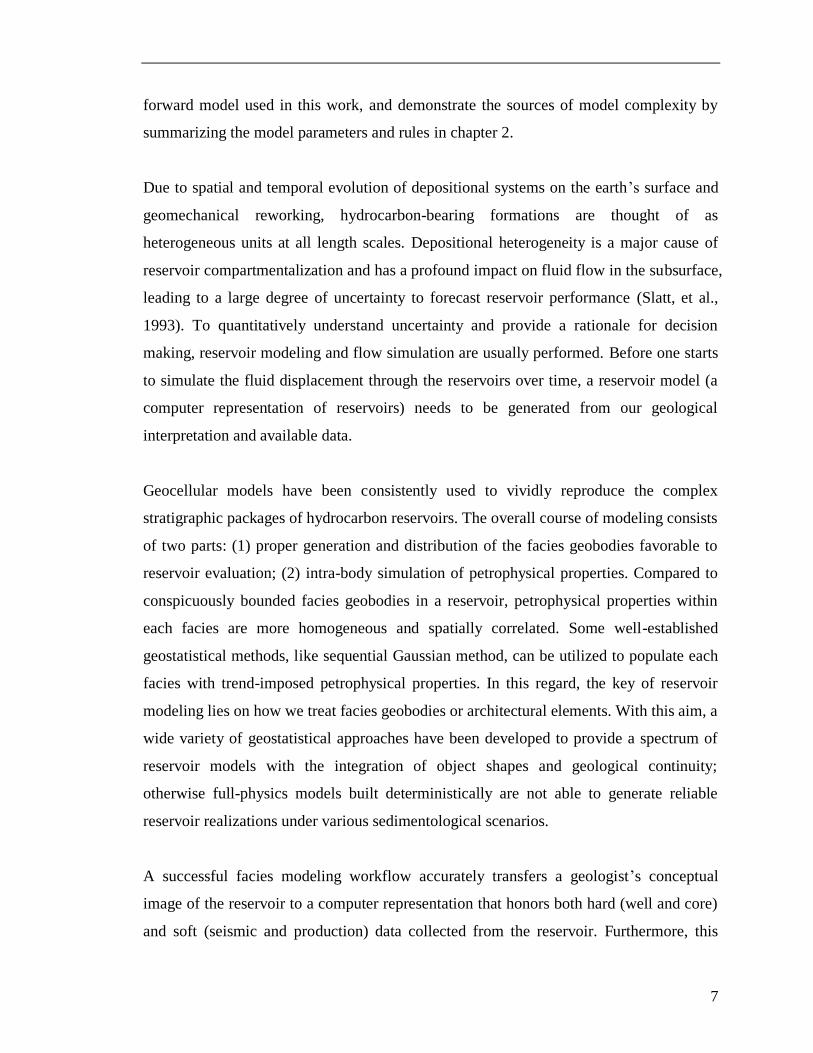
forward model used in this work, and demonstrate the sources of model complexity by
summarizing the model parameters and rules in chapter 2.
Due to spatial and temporal evolution of depositional systems on the earth’s surface and
geomechanical reworking, hydrocarbon-bearing formations are thought of as
heterogeneous units at all length scales. Depositional heterogeneity is a major cause of
reservoir compartmentalization and has a profound impact on fluid flow in the subsurface,
leading to a large degree of uncertainty to forecast reservoir performance (Slatt, et al.,
1993). To quantitatively understand uncertainty and provide a rationale for decision
making, reservoir modeling and flow simulation are usually performed. Before one starts
to simulate the fluid displacement through the reservoirs over time, a reservoir model (a
computer representation of reservoirs) needs to be generated from our geological
interpretation and available data.
Geocellular models have been consistently used to vividly reproduce the complex
stratigraphic packages of hydrocarbon reservoirs. The overall course of modeling consists
of two parts: (1) proper generation and distribution of the facies geobodies favorable to
reservoir evaluation; (2) intra-body simulation of petrophysical properties. Compared to
conspicuously bounded facies geobodies in a reservoir, petrophysical properties within
each facies are more homogeneous and spatially correlated. Some well-established
geostatistical methods, like sequential Gaussian method, can be utilized to populate each
facies with trend-imposed petrophysical properties. In this regard, the key of reservoir
modeling lies on how we treat facies geobodies or architectural elements. With this aim, a
wide variety of geostatistical approaches have been developed to provide a spectrum of
reservoir models with the integration of object shapes and geological continuity;
otherwise full-physics models built deterministically are not able to generate reliable
reservoir realizations under various sedimentological scenarios.
A successful facies modeling workflow accurately transfers a geologist’s conceptual
image of the reservoir to a computer representation that honors both hard (well and core)
and soft (seismic and production) data collected from the reservoir. Furthermore, this
Page 24
8
computer model can be used as a predictive model of spatial heterogeneity and
hydrocarbon recovery. In our study, instead of prediction, the goal of modeling is more
focused on explorative analysis of uncertain predictive results. The modeling methods
have grown to develop out several families during the long-term application of models.
Traditional modeling methods, such as two-point covariance-based approaches excel at
integrating diverse data samples, but they do not honor real sedimentary structures. In
contrast, provided the same data samples, Boolean object-based methods may have
difficulties in data conditioning, but they are able to capture the relationship among
different facies, even if this relationship is restricted and will be repeatedly imposed in
the modeling process without changes. Multiple-point geostatistical modeling turns out to
be more balanced and allows us to incorporate more geological understanding through
training images. However, it is not able to reproduce the spatial and temporal relations
among complex geological processes (Bertoncello, 2011), unless new algorithms can be
coined to flawlessly generate reservoir realizations reflecting overall stationary or non-
stationary features of the training image. Process-based modeling can provide a very
realistic representation of subsurface sedimentary structures by utilizing physical
governing equations to simulate depositional and erosional events over time. The use of
this simulation and related data integration, however, cost huge amount of computation
power as well as time, which does not seem very practical in reservoir characterization
given limited resources and tight schedules. Of course, reduced-physics models have
been developed, but they are largely simplified and can only mimic large-scale geological
events. Besides, they greatly shrink the predictive uncertainty intervals because of
physical assumptions and deterministic output.
The diversity of geomodel families presents a dilemma for modelers. When they perform
modeling, they have to go through a series of tough decisions to sort out a specific
applicable method from existing ones. A systematic way of guiding people to select
modeling methods have not appeared so far. In fact, instead of finding such a way of
selecting, modelers and researchers have been more enthusiastic about creating better
reservoir modeling methods. Surface-based modeling (Pyrcz et al., 2005; Wellner et al.,
2006; Zhang et al., 2009) and rules-based algorithms (McHargue et al., 2010; Sylvester et
Page 25
9
al., 2010) provide promise in capturing realistic geometric evolution of facies geobodies
without the need for complex numerical solutions of process-based models. In addition,
this new method avoids applying advanced algorithms to reproduce training images and
is able to directly translate understandings of depositional mechanics into modeling rules.
Although baffles in data conditioning remain, surface modeling with rule-based
algorithms can be easily implemented because of fast computation if there are only sparse
data available. To this point, it might be an optimal tool to use at the appraisal stage,
especially for a deep-water oil reservoir.
The rules to guide surface-based modeling include two regimes: one regime is directed
toward the types and associated characteristics of facies geobodies; the other regime aims
at controlling the geological processes in relevance to each type of facies geobodies. For
instance, if we try to simulate a channelized system using surface-based modeling, the
first regime of rules describes how many events we have, how many kinds of facies we
have, and what different facies look like. Because the term 'events' has been used a lot in
different contexts, here we explain 'events' as preserved stratigraphic structures formed by
a depositional process during a certain period. A given geologic event is determined
based on the topological and/or geological properties of the geologic volume of interest at
the time of the geologic event, environmental conditions present at the time of the
geologic event that impact geologic formation, deposition, and/or erosion, and/or other
considerations. It is well known that different facies display different depositional
mechanics (Figure 1-4). The rules we use to reproduce these depositional mechanics or
processes belong to the second regime of rules.
Figure 1-4: Demonstration of general rule-based modeling approach
Page 26
10
1.3. Geomorphic Experiments
To capture the realism of lobe deposition and mimic the geologic processes through rule-
based modeling, two geomorphic experiments, DB-03 and TDB-10-1, are utilized. The
initial aim of these experiments is to explore the relation between earth surface processes
and subsurface stratigraphy. By experiments, we are able to obtain a time series of
topographic evolution and resulting stratigraphy of a fluvial deltaic system for
sufficiently long time intervals over which the sediment transport system is able to visit
every spot in a basin repeatedly. This time interval was equal to the time required to
aggrade the bed by a vertical distance equal to about seven channel depths, regardless of
the subsidence rate. This is an advantage of physcial experiments compared to the
limitation of ancient record collected from the natural world.
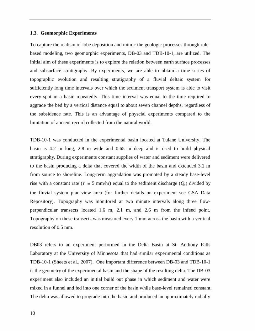
TDB-10-1 was conducted in the experimental basin located at Tulane University. The
basin is 4.2 m long, 2.8 m wide and 0.65 m deep and is used to build physical
stratigraphy. During experiments constant supplies of water and sediment were delivered
to the basin producing a delta that covered the width of the basin and extended 3.1 m
from source to shoreline. Long-term aggradation was promoted by a steady base-level
rise with a constant rate ( r = 5 mm/hr) equal to the sediment discharge (Qs) divided by
the fluvial system plan-view area (for further details on experiment see GSA Data
Repository). Topography was monitored at two minute intervals along three flow-
perpendicular transects located 1.6 m, 2.1 m, and 2.6 m from the infeed point.
Topography on these transects was measured every 1 mm across the basin with a vertical
resolution of 0.5 mm.
DB03 refers to an experiment performed in the Delta Basin at St. Anthony Falls
Laboratory at the University of Minnesota that had similar experimental conditions as
TDB-10-1 (Sheets et al., 2007). One important difference between DB-03 and TDB-10-1
is the geometry of the experimental basin and the shape of the resulting delta. The DB-03
experiment also included an initial build out phase in which sediment and water were
mixed in a funnel and fed into one corner of the basin while base-level remained constant.
The delta was allowed to prograde into the basin and produced an approximately radially
Page 27
11
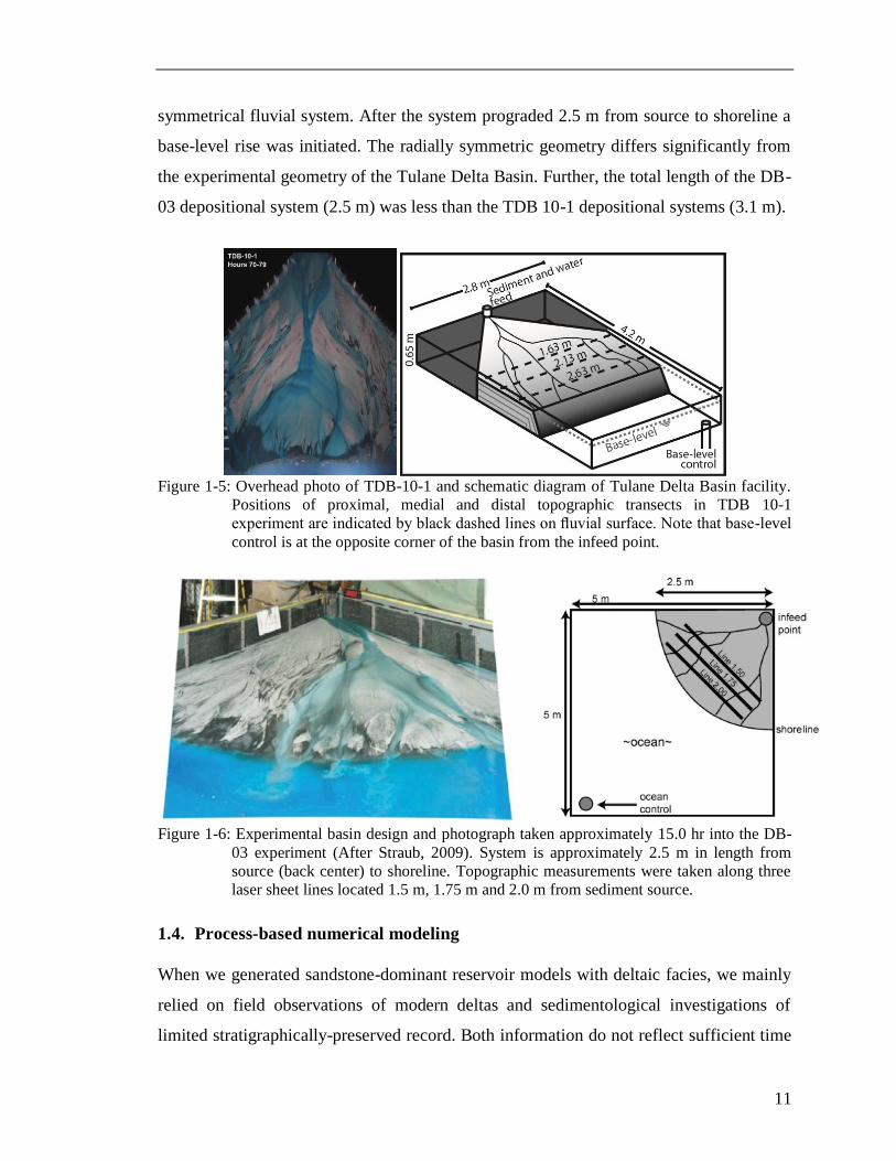
symmetrical fluvial system. After the system prograded 2.5 m from source to shoreline a
base-level rise was initiated. The radially symmetric geometry differs significantly from
the experimental geometry of the Tulane Delta Basin. Further, the total length of the DB-
03 depositional system (2.5 m) was less than the TDB 10-1 depositional systems (3.1 m).
Figure 1-5: Overhead photo of TDB-10-1 and schematic diagram of Tulane Delta Basin facility.
Positions of proximal, medial and distal topographic transects in TDB 10-1
experiment are indicated by black dashed lines on fluvial surface. Note that base-level
control is at the opposite corner of the basin from the infeed point.
Figure 1-6: Experimental basin design and photograph taken approximately 15.0 hr into the DB-
03 experiment (After Straub, 2009). System is approximately 2.5 m in length from
source (back center) to shoreline. Topographic measurements were taken along three
laser sheet lines located 1.5 m, 1.75 m and 2.0 m from sediment source.
1.4. Process-based numerical modeling
When we generated sandstone-dominant reservoir models with deltaic facies, we mainly
relied on field observations of modern deltas and sedimentological investigations of
limited stratigraphically-preserved record. Both information do not reflect sufficient time
Page 28
12
and is not always complete as not all deposited sediments are preserved in an oil reservoir.
Numerical models, provided they are accurate for the scales and processes of interest, can
offer a means to examine the relationship between deltaic river processes and the
resulting morphology or stratigraphy, especially prevailing theories on dominant forcings
and distributary channel network formation (Storms et al., 2007). Continued
developments in process-based hydrodynamic and sediment transport modeling,
especially progress in morphological upscaling methods, have expanded the applicability
of these models to the larger spatial and temporal scales relevant to sedimentary geology,
including simulation of delta development (Storms et al., 2007). To this point, we are
able to build a good numerical reference at the same temporal and spatial scales
consistent with reservoirs. Additionally, we can obtain detailed process data from each
reference at any scale, including time series of forcings and morphologic/stratigraphic
response. Of course, boundary conditions and initial settings on genetic processes will
require significant inferences when using process-based models. In addition, the related
input parameters are too many to apply the process-based tools directly to reservoir
modeling. These hurdles are drivers making us think about combining process-based
models with rule-based models in terms of applicability.
In accordance with the research objective to simulate the morphological development of a
river-dominant reservoir through rules, the coupled hydrodynamic and morphologic
modeling software Delft3D was used to construct a model of typical deltaic river systems.
Delft3D is an integrated modeling suite developed by Deltares and has the capability to
simulate two-dimensional and three-dimensional flow, sediment transport, and
morphological changes. The Delft3D-FLOW module integrates the computation and
interaction of hydrodynamics, sediment transport, and morphology in a simultaneous
approach where hydrodynamics in the next time step would be calculated coupling with
changes to bathymetry in current time step (Figure 1-6 B; Lesser, et al. 2004).
Page 29
13
Figure 1-7: Demonstration of a Delft3D realization and its modeling approach. A) Bathymetry
after 800 days of morphological simulation, applying four parallel runs with 90- phase
shifts and a morphological factor n = 40. B) Flow diagram of morphodynamic model
setup.
Hydrodynamics in Delft3D are simulated by solving the unsteady shallow water
equations on a finite-difference rectilinear, curvilinear, or spherical grid (Lesser, et al.
2004). Though the program is capable of simulating flows in three dimensions, the depth-
averaged mode is implemented for the current study, an assumption justified by the
success of conceptual delta development models using depth-averaged flow conditions.
The sediment transport portion of the FLOW module can compute both bed load and
suspended load transport for non-cohesive sediment fractions and suspended load
transport for cohesive sediment fractions. Suspended transport for both sediment types
follows from the advection-diffusion equation. The erosion and deposition from
suspension of cohesive sediment is calculated according to the Partheniades-Krone
formulations that determine flux to and from the bed based on ratios of bed shear stress to
user-defined critical shear stress values for erosion and deposition. Transport of non-
cohesive sediment is calculated using the formulations of Van Rijn, 1993, the default
sediment transport formula in Delft3D (Deltares 2009). For more detailed information on
the theoretical background, numerical implementation, and practical use of Delft3D,
please refer to the program user manuals and Lesser, et al., 2004 (Lesser, et al. 2004;
Deltares 2009).
The ability of process-based models to simulate delta-development processes and the
resulting morphology/stratigraphy has been established (Edmonds and Slingerland 2007;
Storms et al., 2007). The most recent research in modeling conceptual delta evolution has
Page 30
14
focused on testing the influence of various sediment properties and forcings on the
morphological development. In my work, Delft3D was used to model the initial delta
formation from a river dominant effluent discharging constant flow and sediment loads
into shallow and deep receiving basins under homopycnal conditions. Then the delta
distributary network is generated by the growth of subaqueous levees and mouth bars,
mouth bar stagnation and channel bifurcation, breaching of mouth bars and subaqueous
levees to form multiple bifurcations, and channel avulsion (Figure 1-6 A).
Page 31
15
Chapter 2
2. Rule-based Model Construction
In our study, we perform surface-based modeling with rule algorithms (rule-based
modeling is used in the following chapters) and generate facies geometry in a time
sequence to form 3-dimensional stratigraphy. The basic workflow is to generate the 3-D
geometry of a required geobody (a turbidite lobe or a channel), position it on the
intermediate topographic surface and then update the depositional thickness everywhere
at each time step as a series of geologic events pile up sequentially. Through this
modeling process, we conduct forward modeling that reproduces stratigraphic evolution
of a deep-water turbidite lobe system and deltaic river system through the operation of a
set of input process parameters and algorithms. Parameters and algorithms describe the
behavior of the stratigraphic process response system. In fact, a turbidite lobe system and
a deltaic channel with terminal splays share similar facies unit and morphological
features. Majority of these parameters and algorithms are generalized in a rule-based
modeling flow. Therefore, in this chapter we give an example of channel-lobe models to
show the basic course of modeling facies with rules.
2.1. Rules and Their Classification
Some concepts of 'modeling rules' have been briefly introduced in Chapter 1. Here we
hope to explain a little more and discuss classification of rules in terms of constructive
complexity of computer models. In rule-based modeling, the constructive complexity of
models contains two components - scale of rules and scope of rules. Scale and scope are
probably two of the most overused words in Economics. Scale is about the benefits by the
production of large volume of a product, while scope is linked to benefits by producing a
wide variety of products. In our work, the explanation of scale and scope is slightly
different. Similarly, scale is about numbers and scope is about variety. As for rule-based
modeling, scale is linked to the number of sedimentary facies of different types
represented in models (Figure 2-1). In 1838, Amanz Gressly termed facies a
Page 32
16
distinctive rock unit that forms under certain conditions of sedimentation, reflecting a
particular process or environment. Because sedimentation is associated with time scale of
events, the amount of sediment, and various physical and chemical reworking, the term
scale also foreshadows the size of simulated events. Scope refers to a variety of rules
guiding the sedimentation of each facies (Figure 2-1), including hierarchy integrated in
the models.
Take a model of lobe progradation for example (Figure 2-1). Lots of evidence related to
this sedimentary feature have been found in field research, such as Burdekin River Delta
of northeastern Australia (Fielding, et al., 2006) and Mississippi subdelta-lobe
progradation in Gulf of Mexico (Flocks, et al., 2006). The sedimentation mechanism is
simply that as the progradation goes on, the channel cuts into progradationally stacked
lobe deposits. The number of facies types varies laterally on the matrix in Figure 9, while
the sedimentary processes vary vertically on the matrix. From the left to right, the in-
channel mud drape types increase and the size of filling events decrease. On the first
column, the mud drape could result from two processes - suspended load fallout and
residual lags. Therefore, rows of the matrix represent the variety, namely the scope, and
columns of the matrix represent the scale.
Figure 2-1: Demonstration of scale and scope in rule-based models
Plenty of rules have been created to perform rule-based turbidite lobe modeling (Table 2-
1). Some rules correlated with geobody geometry can be controlled by fixed parameter
values or a probability distribution of the value. However, it is fairly unreasonable to use
some parameter values to define rules associated with depositional processes. These rules
are usually associated with structure in the model. Model structure refers to the behavior
of model components (geological processes) and their interactions. For instance, we
Page 33
17
assume more fine-grain deposits are placed in topographic lows and depositional systems
are preferentially directed to lows, the manifestation of an interaction between these two
components or processes would be that the flow dynamic erosion cuts away all the fine-
grain deposits. Because we apply a hierarchical framework to simulate parent events
(lobe complexes) and offspring events (lobe elements) using different rules, we classify
rules of geological processes into two groups: complex and element. The rationale to
apply a hierarchy of rules results from Straub and Pyles (2012). Compared to offspring
events, parent events may be subject to compensation and relatively strong influence
from topography.
Overall, two families of rules control the modeling process. The first family contributes
to defining the constructive scale, namely the characteristics of architectural elements or
facies, like types, geobody geometry, size and patterns of geological events. The second
family governs the constructive scope, namely system behavior of architectural elements,
for example, the movement, spatial placement, frequency of event occurrence and time
sequence. Even if we group some of rules in one family, these rules function in different
ways. For example, we have stationary rules, like point sediment source rather than line
sources and a channelized segment that always connects with a terminal lobe. These rules
are quite deterministic over the course of modeling. More complex, there are stationary
stochastic rules including the use of probability maps and CDFs. We also have scheduled
rules to make systematic changes without dependence on the current state of model, such
as deterministic rules to control hemipelagic mud. Here we see a great level of
complexity in this rule-based modeling framework.
Rules aim for different objects and behave differently as well. The intermingled nature of
rules reflect the efforts we devote to incorporating geological concepts and reducing
artifacts of models. However, for the downside, the stochastic control and unknown
interaction of rules lead to complex dynamics that is highly variable in space and time,
and thus produce profound uncertainty of outcomes. We know that the origin of
uncertainty is closely correlated with the complexity of systems, but what we do not
grasp is specifically how to describe such a relationship between complexity and
Page 34
18
uncertainty in terms of rule-based modeling. If we attempt to model one facies, we may
largely reduce the variance of our predictions as we increase stochastic rules (e.g.
probability maps) to finely control its sedimentation. However, it is questionable that
whether or not this uncertainty would be reduced when we expect to model one more
type of facies and input more rules constraining its behaviors, namely routing the system
deterministically. In addition, unknown interactions among various modeling rules may
occur during the model construction.
Table 2-1: Summary of rules for rule-based modeling used in our work
2.2. Discussion on Model Complexity
Complex dynamics of a geomodel system with various modeling rules contribute to the
uncertainty of our forecasts. Model parameters, rules and resulting complexity grow at a
significant rate. One reason is that we have been theoretically gaining more and more
understandings on characteristics of sedimentary processes, as we observe, compare and
quantitatively describe geological phenomenon. The other reason is that even though the
model complexity and size are large, we are able to have great model performance during
runs with increasing computational capabilities. Since we have two reasons, it is
seemingly reasonable to increase model complexity if we expect to build the model as
close to reality as possible. However, there are more reasons for us to pursue simpler
Category Objects Rules Representation
Template Geometry Deterministic Equation
Longitutional Length CDF
Aspect Ratio CDF
Depositional Magnitude CDF
Erosional Magnitude CDF
Width CDF
Depositional Magnitude CDF
Erosional Magnitude CDF
Tau Value CDF
Number of complexes CDF
Migration Direction CDF
Progradation Distance CDF
Retrogradation Distance CDF
Lateral Shifting Distance CDF
Number of Offspring Elements CDF
Frequency Deterministic Set of Rules
Thickness Deterministic Set of Rules
Influence of Topography Deterministic Set of Rules
Facies Geobody Geometry
Geological Processes
Terminal splays
Proximal Channels
Complex
Element
Hemipelagic Shale
Page 35
19
models for our purpose. First of all, simpler models are easier to implement, validate and
analyze. If we can build a single facies to tackle our problem, we can avoid so many
model settings instead of building two facies. Secondly, modelers tend to throw in more
possible factors, reflecting the lack of understanding of the real system. In this case, we
doubt that the model responses could approximate the reality. Likewise, statisticians have
found overly complex regression models may lead to data overfitting. Thirdly,
requirements of complexity largely increase the risks for modelers to incorrectly translate
a conceptual model into a computerized model. In addition, if we are going to update our
models and hypothesis given new data, it is certainly easier to change a simple model
rather than a complex model. Now the point is whether we want to integrate everything
that we know to make our model a 'know it all', or we expect to feed models up with
necessary knowledge to encourage a 'diet'.
If we are going to create a combined process-based and rule-based workflow to focus on
analysis of uncertainties of production predictions, thus reducing the history matching
effort and other manual modeling intervention,we may need to simplify process-based
models first. This means to determine those geological process-model parameters
impacting reservoir performance before developing rules from process-based models.
This can be done by integration with some prior information (well and seismic data) and
a global sensitivity analysis over the parameter space.
2.3. Modeling A Typical Channel-lobe System
Details of constructing a rule-based model have been described and explained in a few
previous studies (Leiva, 2009; Xu, 2014). However, most of those are focused on
defining the facies shapes of a single depositional system and a variety of deterministic
and stochastic stationary rules used for assigning kinetics to this single system. Recently,
high-resolution seismic studies (e.g. Piper et al., 1999; Gervais et al., 2006; Deptuck et al.,
2008) and detailed outcrop studies (Prélat et al., 2009; MacDonald et al., 2011) have
found that the down-dip portion of some sand-rich submarine lobes and lobe-like jet
deposits in the formation of deltas are well-organized, and can be hierarchically sub-
divided into a number of higher-order and lower-order units. This division has resulted in
Page 36
20
development of comparable four-fold hierarchies where beds and bedsets stack into lobe
elements, lobe elements stack into lobes and composite lobes stack into lobe complexes
(Grundvag et al., 2014). Therefore, a set of rules for modeling a single flow event or a
single depositional system is not enough. A hierarchical concept should be embedded into
the model structure.
Figure 2-2: Demonstration of hierarchical framework imposed in the forward modeling.
In this report we propose a scheme to build a hierarchical channel-lobe system using rule-
based model approach. Different rules will be developed for different hierarchies based
on the proposed conceptual model and field work conducted by Straub and Pyles in 2012.
The scheme of forward modeling includes three steps: (1) determining the position of the
parent system, (2) simulating the offspring events anchored at parents and (3) generating
stacked surfaces. Noted that the parent system and offspring system are relative terms
here. The parent system refers to a spatially large-scale depositional system with
relatively complex architecture, while the offspring system refers to small-scale events
that fill up the space of a parent system (Figure 2-2). If we consider a lobe complex as a
parent event, composite lobes would be the offspring events; likewise, if we consider a
composite lobe as a parent event, lobe elements would be the offspring events. Deptuck
(2008) demonstrated the lobe classification as: lobe complex (50 to >100 ky), composite
lobe (10 to 14 ky), lobe element (<5 ky) and bed to bed set (hours to days). Straub and
Page 37
21
Pyles (2012) proved that submarine lobes behave differently and result in distinct
stacking patterns at different scales. In contrast to offspring events, parent events tend to
compensate the topographic reliefs.
2.3.1. Compensational Stacking
Compensational stacking is defined as the tendency of sediment transport processes to fill
in topographic lows through deposition. This tendency is thought to result from periodic
reorganization of the sediment transport field to minimize potential energy associated
with elevation gradients (Mutti and Sonnino, 1981; Deptuck et al., 2008).
Compensational stacking has been used to describe large-scale architecture in deepwater,
fluvial, and, deltaic packages (Mohrig et al., 2000; Olariu and Bhattacharya, 2006;
Hofmann et al., 2011), wherein avulsions reorganize the sediment transport field along
local topographic lows. In our study, this concept is translated into rules to control the
modeling of parent events.
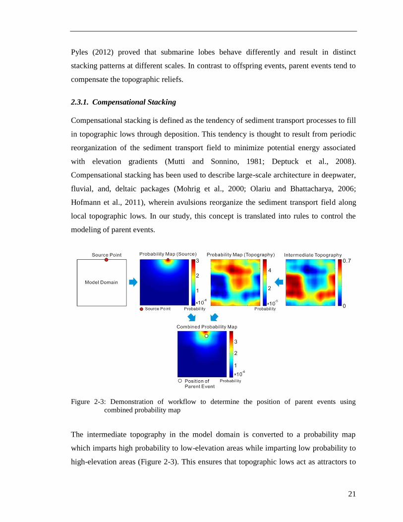
Figure 2-3: Demonstration of workflow to determine the position of parent events using
combined probability map
The intermediate topography in the model domain is converted to a probability map
which imparts high probability to low-elevation areas while imparting low probability to
high-elevation areas (Figure 2-3). This ensures that topographic lows act as attractors to
Page 38
22
parent events leading to an evenness of the system. Besides, deposits tend to settle in the
proximal location. Based on the Euclidian distance to the source point or sediment infeed
point, we are able to generate a distance map in the model domain and then convert this
distance map into a second probability map. To merge proximal deposition rule and
compensational stacking rule, we produce a combined probability map through a
weighted mean of two generated probability maps (Figure 2-3). This combined
probability map allows us to sample a location for a parent event under the guidance of
geological concepts - compensation and proximal deposition.
Once the location of a parent event is found, we conduct another workflow to fulfill the
positioning of offspring events. These offspring events are treated as internal fillings of
the parent event. Thus, spatial location of offsprings would be conditioned to where the
parent is located. Each offspring event consists of a terminal splay and a channel in terms
of deposited geobodies. This pattern mimics a depositional process that turbidite currents
coming out from the source point detach deposits in the model domain, leaving a scour
channel filled with fine sands and a lobe at the end of channel where currents lose the
confinement.
We adopt a centerline algorithm to generate offspring events. This algorithm has been
used to mimic the sinuous pattern of fluvial and submarine channels and simulate channel
migration over time. The configuration of a centerline is controlled by a set of nodes
distributed along the centerline trace. Usually in a kinetic channel evolution model, the
movement of each node along the centerline is governed by a migration rate that is linked
to the flow field (Yi, 2006). Instead of manipulating the depositional processes as in
process-based models, we use five nodes along a centerline to shape the sinuosity of
overall system with statistical rules and create different facies shapes (the channel and
lobe) on different segments between nodes. From the proximal to distal location, we
name the five nodes as source point, channel center point, junction, lobe center point and
terminal (Figure 2-4). Source point refers to the sediment infeed point, channel center
point refers to the control node in the middle of the channelized segment in the proximal
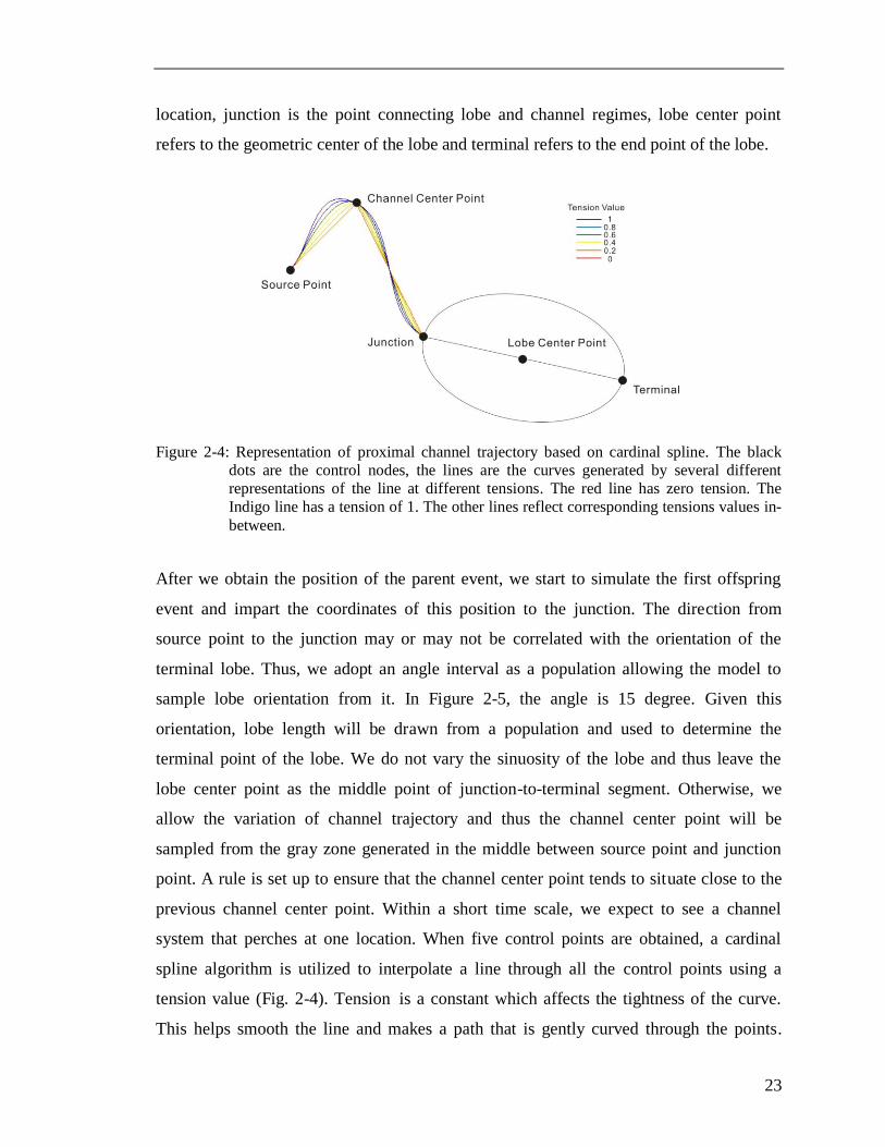
Page 39
23
location, junction is the point connecting lobe and channel regimes, lobe center point
refers to the geometric center of the lobe and terminal refers to the end point of the lobe.
Figure 2-4: Representation of proximal channel trajectory based on cardinal spline. The black
dots are the control nodes, the lines are the curves generated by several different
representations of the line at different tensions. The red line has zero tension. The
Indigo line has a tension of 1. The other lines reflect corresponding tensions values in-
between.
After we obtain the position of the parent event, we start to simulate the first offspring
event and impart the coordinates of this position to the junction. The direction from
source point to the junction may or may not be correlated with the orientation of the
terminal lobe. Thus, we adopt an angle interval as a population allowing the model to
sample lobe orientation from it. In Figure 2-5, the angle is 15 degree. Given this
orientation, lobe length will be drawn from a population and used to determine the
terminal point of the lobe. We do not vary the sinuosity of the lobe and thus leave the
lobe center point as the middle point of junction-to-terminal segment. Otherwise, we
allow the variation of channel trajectory and thus the channel center point will be
sampled from the gray zone generated in the middle between source point and junction
point. A rule is set up to ensure that the channel center point tends to situate close to the
previous channel center point. Within a short time scale, we expect to see a channel
system that perches at one location. When five control points are obtained, a cardinal
spline algorithm is utilized to interpolate a line through all the control points using a
tension value (Fig. 2-4). Tension is a constant which affects the tightness of the curve.
This helps smooth the line and makes a path that is gently curved through the points.
Page 40
24
Through cardinal spline and the position of channel center point, we are able to
manipulate the shape of channel trajectory.
We represent a centerline going across five control points that define the turbidite lobe
system (Fig. 2-5). The shape of the system is computed based on the distance to the
centerline. Figure 2-5 shows a pair of blue curves on two sides of the red centerline.
These blue curves indicate the edges of the proximal channelized segment of the channel-
lobe system. The distance between the borderlines is scaled to the width of channel that is
defined in the model setting. Thickness of channelized deposition is computed based on
the distance away from the centerline and approaches zero while meeting the borderlines.
An elliptical shape is generated around the centerline segment between the junction and
the terminal. It mimics the boundary shape of a terminal lobe and is marked by a yellow
line on Figure 2-5. Thickness of lobe deposition is computed based on the distance away
from the junction point and approach zero while meeting the lobe boundary. A thickness
map for a single offspring event is demonstrated in Figure 2-5.
Figure 2-5: Demonstration of generating a single event using surface-based modeling
2.3.2. Clustered Stacking
Between two parent events, the whole depositional system settles down and tries to even
out the low-elevation areas in the basin. A correlation is imposed by adding rules among
offspring events that belong to one cluster. The coordinates of the junction point will be
recorded every time step. These coordinates are used to identify the position of the
Page 41
25
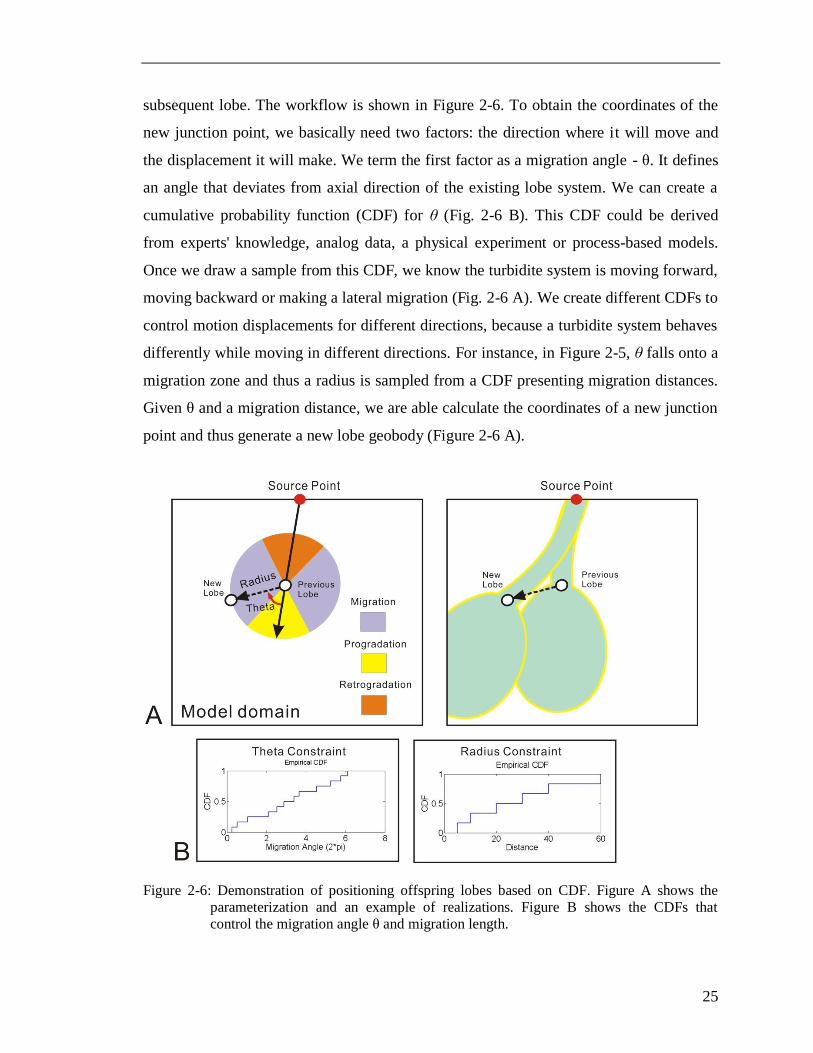
subsequent lobe. The workflow is shown in Figure 2-6. To obtain the coordinates of the
new junction point, we basically need two factors: the direction where it will move and
the displacement it will make. We term the first factor as a migration angle - θ. It defines
an angle that deviates from axial direction of the existing lobe system. We can create a
cumulative probability function (CDF) for θ (Fig. 2-6 B). This CDF could be derived
from experts' knowledge, analog data, a physical experiment or process-based models.
Once we draw a sample from this CDF, we know the turbidite system is moving forward,
moving backward or making a lateral migration (Fig. 2-6 A). We create different CDFs to
control motion displacements for different directions, because a turbidite system behaves
differently while moving in different directions. For instance, in Figure 2-5, θ falls onto a
migration zone and thus a radius is sampled from a CDF presenting migration distances.
Given θ and a migration distance, we are able calculate the coordinates of a new junction
point and thus generate a new lobe geobody (Figure 2-6 A).
Figure 2-6: Demonstration of positioning offspring lobes based on CDF. Figure A shows the
parameterization and an example of realizations. Figure B shows the CDFs that
control the migration angle θ and migration length.
Page 42
26
In the same manner, we generate a series of offspring lobes. These lobe are spatially
correlated with each other and form a more complex system in the stratigraphy, namely a
parent event. When the simulation of offspring lobes ends for a parent event, the
subsequent parent event will be determined depending on the combined probability map
that is updated by integrating new topography and source point. This rule would help the
depositional system behaves accordingly to respond to topographical evolution through
time, which is usually observed as migration of depositional center in the stratigraphic
record. For the purpose of demonstration, we sequentially simulate five lobe complexes
(Figure 2-7). Over the course of simulation, it is observed that the lobe system would be
perched at a location for a while, and then it mimics a regional avulsion, migrate to
another location and start to pile up once again.
2.4. Rasterizing Rule-based Models
A complete workflow to forecast reservoir performance using rule-based modeling
include defining modeling rules through settings, generating realizations, gridding surface
models, assigning categorical variables, simulating petrophysical properties, upscaling
models and simulating water flooding. When needed rules are embedded in the model
settings, we generated surface-based models demonstrating stratigraphy that contains pre-
defined architectural elements. These elements or geobodies are represented by smooth
and continuous surfaces and are constructed on the unstructured grid. In order to run flow
simulation, the resulting models must be vertically discretized depending on a grid size.
On Figure 2-8, a turbidite channel-lobe model is converted from 3D stacked surfaces to a
volumetric cube. During this conversion, we use indicator variables to represent and
differentiate each facies, forming a basis for subsequent petrophysical modeling. The
volumetric cube of a surface model will be input to Petrel where porosity and
permeability will be assigned to each cell based on Sequential Gaussian Simulation
(SGS). We can perform upscaling using Petrel and then input an upscaled model to
Eclipse for flow simulation.
Page 43
27
Figure 2-7: Depositional maps of one single flow event, a cluster and five clusters. Transition of
depositional maps represents a hierarchical construction embedded in rule-based
modeling. The channel-lobe offspring events only try to fill up a local space until the
external conditions change redirecting the system.
Figure 2-8: Workflow to convert surfaces to volumetric data for flow simulation. We discretize
each continuous surface that envelops different facies bodies, and assign a
distinguishable indicator to each facies. If we slice the volumetric data from bottom
top, we can observe a systematic evolution.
Page 44
28
Chapter 3
3. Modeling Turbidite Lobes with Experimental Data
Deep-water turbidite lobe systems have been one of the most important hydrocarbon
reservoirs in the subsurface. However, seismic imaging and sparse well data lead to a
high uncertainty level in the resource exploration and development. Understanding this
uncertainty of reservoir heterogeneities in a lobe system often requires stochastic models
of sub-seismic features. We present a simulation algorithm connecting stratigraphic
organization with surface-based reservoir models through statistical metrics. Information
of stratigraphic organization is extracted from geomorphic experiments. In our study, a
lobe classification scheme and Ripley’s K-function are utilized to extract information
about sub-seismic lobe element organization from experimental strata. We utilize these
two metrics in conjunction with a rule-based simulation algorithm to 1) integrate
clustering patterns of turbidite lobes into reservoir modeling 2) reproduce a numerical
stratigraphic framework comparable to physical geomorphic experiments 3) explore a
means of imparting stochastic structures to models and improving geological realism.
3.1. Methodology Overview
When we search for useful information in a set of geomorphic experiments, the
prerequisite of 'useful' is 'comparable' in terms of scales because the topographic
evolution occurs in an experimental basin not a natural basin. However, finding
comparable information requires time-consuming theoretical and empirical work. Instead
of doing this, an alternative solution has been developed to behave as a shortcut. The
solution is to select the experiment as similar to the system of the reservoir as possible to
provide information for reservoir modeling (Xu, 2014). It estimates a similarity between
lobe stacking patterns of two systems, which are characterized by the cumulative
distribution functions of pairwise lobate proximity measurements (Xu, 2014). The
similarity is estimated with a bootstrap two-sample hypothesis test on the two cumulative
distribution functions. Since lobate bodies in experiments can be identified hierarchically
Page 45
29
from small scales to large scales depending on decisions of the interpreter, the solution
also includes an automatic method to quantify lobe hierarchies and to choose lobate
stacking patterns at various scales of interpretation. In our study this solution is applied to
estimate the similarity between two delta fan experiments, TDB-10-1 and DB-03. We
interpret lobe deposits of multiple scales for TDB-10-1 while only large scale deposits are
interpreted in DB-03. Based on statistical similarity analysis, an experimental lobe pattern
at a certain interpretation resolution in TDB-10-1 was identified as the pattern with the
highest similarity to the lobe stacking structure in DB-03.
Figure 3-1: Demonstration of workflow for reservoir modeling using experimental data
Dendrogram analysis (Figure 3-1) has facilitated a correlation framework that has been
quantitatively interpreted to demonstrate the similarity between a physical tank
experiment and a real depositional system (Xu, 2014). Agglomerative hierarchical
clustering is performed to characterize the internal hierarchy of experimental data.
Through this method Xu quantitatively evaluate the similarity between lobe stacking
patterns in different systems. Because our study is aimed at integration of experimental
data in reservoir modeling, we examine the similarity between experimental stratigraphy
and interpreted field data. We are able to determine which tank experiment at what
Page 46
30
interpretation scale is comparable with available field data by performing a search
through the hierarchy of interpretable lobes. Then characteristics of experimental lobes
below the comparable scale are informative in terms of inferring sub-resolution small-
scale features from visible large scale features. To show an example in our work, we use
DB-03 to indicate a set of field data.
3.2. Quantitative Metric
We identify all the lobe deposits from large scale to small scale in TDB-10-1. The
interpretation is performed based on the geometry of lobes. The largest lobe element is
0.8 meter in width and 1.2 meter in length while the smallest single lobe is 0.2 meter in
width and 0.5 meter in length. Some examples are shown in Figure 3-2. If we use the
proximal point of each lobe to represent its location, a lobe complex can be represented
by a spatial point pattern because a lobe complex is treated as a large scale lobe and
usually consists of multiple smaller scale lobe elements. By performing dendrogram
analysis based on pairwise lobate proximity measurements, we can see a varying point
patterns across the classification tree (Figure 3-3). Each lobe complex can be represented
by a cluster of points. Dendrogram analysis provides us a tree-based archive that stores
information of spatial point patterns over a range of interpretation resolutions.
Figure 3-2: Demonstration of lobe elements in TDB-10-1.
Page 47
31
Figure 3-3: Demonstration of tree structure showing hierarchy of multi-scale lobes. Blue dots
indicate the proximal points of lobe elements. Pink dot represents the center of a
pattern of lobe elements.
Figure 3-4: Demonstration of spatial points indicating center locations of preserved lobe
complexes. Points are associated with a time sequence depending on their depositional
sequence.
We treat the spatial distribution of lobes as a spatial incident point process, providing an
opportunity for surface-based simulation algorithm to link stratigraphic hierarchy with
Page 48
32
reservoir modeling through a spatial statistical metric (Figure 3-4). The point process not
only gives us information regarding a spatial organization of lobes, but also a temporal
formation process of each lobe.
We adopt Ripley's K function (Hajek et al., 2010) to analyze the spatial pattern of
incident point data. Ripley’s K function summarizes spatial dependence (feature
clustering or feature dispersion) over a range of distances. This metric provides a way to
extract information of sedimentary hierarchy and lobe element organization from a set of
experimental strata, and bridge physical tank experiments with numerical models.
Ripley’s K function is given by
j ij
ij
w
d
i
d
2
)(I
n
r = (d)K̂ (3-1)
where r indicates the area of study region, n represents the number of events, dij
represents the distance between the i-th and j-th event, Id is an indicator function that
takes on the value of one if dij<=d, and wij is a correction factor for edge effects . Given a
physical experiment recording the entire evolution of the lobe system, we are able to
transform all the lobes that appear in the geologic time into a spatio-temporal point
process. This point process provides both spatial and temporal information for the growth
of lobes.
3.3. Analyzing Experimental Data
To perform an application of spatial point process, we utilized two physical tank
experiments: TDB-10-1 and DB-03. The TDB-10-1 experiment was conducted at Tulane
Sediment Dynamics Laboratory and modeled on the DB-03 experiment detailed in Sheets
et al. (2007), but had the added aim of generating a stratigraphic package 2-3 times
thicker than the DB-03 experiment. DB-03 was conducted in the Delta Basin at St.
Anthony Falls Laboratory at the University of Minnesota (Sheets et al., 2007; Xu, 2014).
Both TDB-10-1 and DB-03 were conducted with constant allogenic forcings. The
allogenic forcings in the DB-03 experiment, including Qs, Qw and the rate of base-level
rise were identical to TDB 10-1. However, because two different basins were used, DB-
Page 49
33
03 and TDB-10-1 are different in terms of depositional geometry of stratigraphic
packages (Figure 3-5). Figure 3-5 shows the basin geometry and an overhead photo of
TDB-10-1. Details regarding DB-03 are demonstrated in Xu (2014).
Figure 3-5: Demonstration of spatial points indicating locations of preserved lobe complexes. A)
Schematic diagram of Tulane Delta Basin facility. Positions of proximal, medial and
distal topographic transects in TDB 10-1 experiment are indicated by red lines on
fluvial surface. B) Overhead photograph taken at 76 hours into the aggradational
phase of TDB 10-1 experiment. Flow is dyed blue to aid visualization. System is
approximately 3.1 m in length from source to shoreline. The locations of major large-
scale lobes are marked by red dots.
By interpreting the overhead photos of DB-03, we create a lobe system that contains 13
lobe complexes. This lobe system is treated as observable pseudo field data, and we have
not continued to interpret the lobe elements that may exist in complexes. Conversely, we
performed a rather detailed interpretation throughout the experimental stratigraphy of
TDB-10-1. To create an archive containing sedimentary information over all the
interpretable scales, we initiated our interpretation from relatively small-scale lobes (axial
length approximating 0.3 m), and then assembled small-scale lobes to medium-scale
(axial length approximating 0.8 m) and large-scale lobes (axial length approximating 1.2
m). The interpretation and geometry extraction procedures are described with more
details in Xu (2014). Through a comparability searching (Figure 3-1), a lobe stacking
Page 50
34
pattern that we interpreted at a certain scale from TDB-10-1 is found to be of similar
characteristics with the lobe system in DB-03. In our study we term features at this
comparable scale as large-scale information in TDB-10-1. Below this large scale, it is
fairly convenient to extract medium and small scale lobe features, including lobe
geometry and spatial distribution, from our archive.
As demonstrated in Figure 3-5 B, we highlighted the center of large-scale lobes with red
dots in a square domain in Figure 3-6 A. Each red dot refers to a location record of a
large-scale lobe or a lobe complex in space. If we consider these lobe complexes as
parent events, there are relatively fine-scale offspring events filling up each parent event.
These offspring events are often considered sub-seismic lobe elements in seismic imaging.
In our case, the medium and small scale lobes we characterized from TDB-10-1 represent
sub-resolution sedimentary features. Our tree-based archive is capable of providing
information at any scale below the large scale (Figure 3-6).
Figure 3-6: Demonstration of Ripley's K plots at three major interpretation scales.
Page 51
35
All the points that represent small and medium scale lobes are marked by blue dots in
Figure 3-6. We utilized Ripley's K function to evaluate the clustering strength of red dots
and blue dots depending on the measurement length - d (Eq. 3-1). This measurement
length represents distance from random points to their nearest neighbors. The simplest
use of Ripley’s K(d) function is to test complete spatial randomness (CSR). If so, then
K(d)= πd2. In practice, it is easier to use its normalized estimator - Besag’s L function:
d
(d)K̂ = (d)L̂ (3-2)
The advantage of this transformation is that, under the null hypothesis of CSR, the
derived L function has an expectation of 0 for all values of d (Skarpe, 1991). The
resulting plots are more informative and also yield a much higher resolution (Figure 3-4).
In order to illustrate the scales of statistical significance, we generated a confidence
envelop dyed by gray in Figure 3-6. This envelop is approximated by averaging 100 point
patterns that include the existing sampled points and 99 Monte Carlo simulations with the
same point number. The gray-dyed confidence envelope describes a point process where
point events at every measurement scale occur in a completely random fashion. If the
deviation of the sample statistic from zero expectation is positive, and above the upper
limit of the confidence envelope, a clustered distribution of the sampled points can be
assumed, while negative deviation indicates a dispersed or regular pattern. If the sample
statistic remains within the bounds of the confidence envelope for any given t, the null
hypothesis of complete spatial randomness cannot be rejected (Haase, 1995).
3.4. Modeling Sub-resolution Lobes
Ripley's K function allows us to quantitatively describe a distributary turbidite lobe
system from an angle of spatial point process. When we have some observations on
parent events from available data, we are able to transfer the spatial distribution and time
sequence of these parent events into modeling rules, making models conditional to
observable information (Figure 3-7). The point process characterized by K function
provides features of offspring point clusters at different scales, such as the average radius
Page 52
36
of blue dot clusters and the average number of offspring events that occur in the domain
of each parent event (Figure 3-7). In addition, we adjust the geometry of turbidite lobes
during simulation based on width and length CDFs of lobes at different scales.
Figure 3-7: Model inputs and associated realization demonstration. L indicates the size of lobe
clusters and N provides the number of offspring events. The time sequence of large-
scale lobe complexes is transformed into modeling rules to control the time order of
lobe cluster generation. The cluster patterns of small-scale and medium-scale lobes
depend on our interpretation of lobe locations in TDB-10-1. The Black dotes in
realizations denotes locations of generated lobe elements in the simulation.
When we incorporate a point process into the model, the resulting stratigraphy is
characteristic of lobe clusters whereby each cluster would be recognized as a parent event
that is visible in our seismic data. Meanwhile the lobe complexes in the model
stratigraphy match the location and temporal order of each parent event because
observable events are utilized as model inputs. A comparison of model inputs and results
is illustrated in Figure 3-8. It demonstrates less bias on clustering areas, but as we
Page 53
37
increase measurement length and step into blank areas without so many points,
simulation results differ from the original inputs. If we consider those blank areas as
places of no interest in terms of reservoir forecasting, our modeling workflow provides
promise in capturing the hierarchy of turbidite lobes as a whole.
Figure 3-8: Comparison between K functions of inputs and modeling results.
3.5. Discussion
Our modeling method is relatively straightforward and allows us to control the
stratigraphic patterns globally. However, this approach requires a data source providing a
high-resolution interpretation on spatial locations of lobe elements, if we expect the
modeling to assist with forecasting sub-seismic features. Both seismic data and well data
have limitations. Thus, tank experiments and process-based models are very helpful
sources to provide inputs for modeling small-scale stratigraphic features. However as far
as tank experiments are concerned, no one has proved that they contain informative
contents that are exactly the same with natural systems though they have some degree of
geometric similarity. A rationale is still needed to directly use experimental data and
process-based models to infer stratigraphic information in the real reservoirs.
Page 54
38
Chapter 4
4. Feature Extraction of Process-based Models
Geological features in the pattern of deltaic channel networks, such as morphologic
changes in channel shape, branching pattern, width, tortuosity, or the appearance of
related facies, are associated with the occurrence of internal and external environments.
The responses obtained from different types of distributary channel networks are variable
through time resulting in different stratigraphic patterns that strongly affect subsurface
heterogeneities. To incorporate the dynamic formation of strata in reservoir models for
uncertainty quantification, we introduce process-based models that complement voids of
physical understandings ignored in the regular geostatistical modeling approach.
Because the dimension and shapes of channel system continuously vary during the course
of process-based simulation, we make an effort to find an automated, optimal, highly
accurate, and relatively less time-consuming solution for extracting channel features from
model results. A feature extraction algorithm is introduced from image processing of
retinal blood vessels to our problem. Image-based diagnosis has started since 1990s, but
the motivation to analyze process-based delta model for reservoir forecasting was just
triggered several years ago. In addition, the method we need should be sensitive to
channel morphology and a web-like network structure. This also gives us a good reason
to narrow down our search space to vessel identification tools.
The algorithms based on pattern recognition concern with the automatic detection or
classification of retinal blood vessel features and other non vessel objects including
background. Pattern recognition techniques for blood vessel segmentation are classified
into two categories; supervised methods and unsupervised methods. Supervised methods
utilize some preliminary labeling knowledge to decide whether a pixel belongs to a blood
vessel or not whereas unsupervised methods perform the vessel segmentation of blood
vessel without any preliminary labeling information. In unsupervised segmentation, the
Page 55
39
vessel network is detected using pixel-based processing methods through spatial
transformations or tracking operations. The tree-like geometry of the vessel network
makes it a usable feature for registration between objects of a different nature. In order to
discriminate vessels from similar background patterns, a cross-curvature evaluation is
performed. Recently, a new technique, multi-scale line tracking algorithm (MSLTA), has
been developed to extract vessels in retinal images, improving the detection rate of low-
contrast and narrow vessels, decreasing also the false detections at non-vascular
structures. The core of this technique is a new likelihood ratio test that combines
matched-filter responses at different widths, confidence measures defined as a vector
projection of the normalized brightness at each pixel neighborhood onto a vessel profile
and vessel boundary measures. The new likelihood ratio is embedded into a vessel tracing
framework, resulting in an efficient and effective vessel centerline extraction algorithm.
In this chapter, an automated algorithm built on MSLTA for channel network extraction
is presented and evaluated. Our work is focused on how to tackle the problems of the
fully automatic and robust segmentation of the channel network in case of noisy process-
based topography images.
The remaining of this chapter is organized as follows. In Section 1, a necessity to extract
channel networks is presented. The channel network extraction in our study contains two
phases: pre-processing and post-processing. Section 2 contains line tracking, namely pre-
processing, we used for our process-based models. Section 3 contains post-processing,
namely image processing techniques. The experimental evaluation of overall multi-scale
line tracking algorithm is presented and discussed in Section 4.
4.1. Network Skeleton
Distributary channels are described from deep-sea fans (Damuth et al. 1983; Posamentier
and Kolla 2003), alluvial fans (Prior and Bornhold 1990), and delta plains and form when
the main channel reaches an area with low variability of lateral gradient. Because delta-
plain gradients are small and sedimentation rates are high, the direction of distributary
channels can be changed easily by aggradation or differential subsidence and compaction,
Page 56
40
such that the gradient will be steeper in other directions and might capture part of the
flow, creating a new distributary channel (Olariu & Bhattacharya, 2006).
In many modern deltas, the discharge from the ‘‘trunk’’ channel is split into a few major
distributaries, each with different discharges. The main distributaries bifurcate farther
downstream, and with each the discharge and sediment load is split between newly
formed channels. As a consequence of this successive splitting, the distributary channels
become smaller in the downstream direction. Apparently the geometry and types of
channel deposits change downstream as river discharge splits. Before modeling the
details of deposits, a global control of channel network is needed, as this governs the
spatial distribution of all kinds of deposits along the network. Therefore, recognizing and
describing the network structure is a must before we transform network pattern evolution
into modeling rules for forward models.
There are some modern examples from river-dominated deltas showing a process-based
analysis of distribution and dimensions of specific morphometric features and the
formation of terminal distributary channels. Smart (1971) conducted a topology analysis
on channel network skeleton for five natural deltas including Colville, Irrawaddy, Yukon,
Niger and Parana. Hanegan (2011) performed a morphological and dynamic study on
Wax Lake Delta, and reproduced its evolution in Delft3D. Wake Lake Delta (Figure 4-1),
is located in St. Mary Parish along the Gulf Coast in Louisiana. The delta receives its
flow from the Atchafalaya River diversion, a man-made channel 20 km upstream of
Morgan City Louisiana. The delta has been forming naturally, although caused by the
man-made river diversion, since 1973 making it an ideal location for the study of delta
evolution and processes. The delta front has prograded seaward into the Atchafalaya Bay
at a rate of ~0.27 km/yr. A channel network skeleton of Wax Lake Delta was manually
interpreted from a satellite image to perform a hydrodynamic calibration (Figure 4-1).
Other than the skeleton, huge amount of field data have been collected to generate a
process-based delta model.
Page 57
41
Figure 4-1: Satellite image of current Wax Lake Delta and its channel network skeleton (After
Hanegan, 2011).
Differing from satellite image analysis, we face up to a set of 2-D topography images that
describe a life of a river-dominated delta growth. Without measurements of similar
modern deltas for reference, we propose an idea of building a database of process-based
delta models covering all the possible ranges of hydrodynamic parameters. Therefore, we
need an automated and robust feature extraction tool to identify channel network patterns
across hundreds or thousands of topography images from process-based models.
Figure 4-2: Demonstration of topography time series in a process-based delta model (Courtesy of
Wietse van de Lageweg). From left to right, we observed a delta growth process with
a deltaic river network expanding gradually.
4.2. Pre-processing of Topography Images
Delft3D can generate very realistic deltaic river systems by setting up appropriate
physical conditions. The pixel-based topography images are exported at each time step
for pre-processing procedure. This procedure mainly include the utilization of multi-scale
line tracking algorithm (MSLTA) that belongs to the family of unsupervised feature
extraction methods. The multi-scale analysis facilitates the channel feature detection at
Page 58
42
different widths avoiding also the detection of noisy channel-like structures, and
brightness variations.
4.2.1. Supervised and Unsupervised Segmentation Methods
Because MSLTA is developed for channel feature based on retinal vessel detection, we
would like to briefly present a review of vessel segmentation algorithms in this section.
In supervised methods the rule for vessel extraction is learned by the algorithm on the
basis of a segmented reference images and training set of manually processed images.
The reference image is generally termed as the gold standard. The vascular structure in
these ground truth or gold standard images is precisely marked by an ophthalmologist.
But there is significant disagreement in the identification of vessels even amongst expert
observers. In a supervised method the rules for evaluation of result are determined by the
ground truth data. Therefore the prior requirement is the availability of the already
classified ground truth data which may not be available in real life applications. Because
these supervised methods are designed based on pre-classified data, their performance is
usually better than that of unsupervised ones and can produce very good results for
healthy retinal images (Karale and Deshpande, 2015).
The assumption that vessels are elongated structures is the basis for the supervised
method of ridge-based vessel detection and segmentation which was introduced by Staal
et al. The image ridges which roughly coincide with the vessel center lines are extracted
by this algorithm. Soares et al. applied complex Gabor filters for feature extraction and
supervised classification for the detection of blood vessels in retinal fundus images. In
this method the magnitude outputs at several scales obtained from 2D complex Gabor
filters were assigned to each pixel as a feature vector. Then a Bayesian classifier was
applied for classification of the results into vessel or no vessel pixels. Marin et al.
presented a supervised method for blood vessel detection in digital retinal images. This
method uses a neural network (NN) scheme for classification of pixels
The techniques based on unsupervised classification seeks to find inherent patterns of
Page 59
43
blood vessels in retinal images that can then be used to decide that a particular pixel
belongs to vessel or not. The training data or hand labeled ground truths do not contribute
directly to the design of the algorithm in these techniques. Salem et al. proposed a Radius
based Clustering Algorithm (RACAL) which uses a distance based principle to represent
the distributions of the image pixels. A partial supervision strategy is combined with the
clustering algorithm. Unsupervised methods for automatic vessel segmentation from
retinal images are attractive when only small datasets with associated ground truth
markings are available. Garg et al. proposed an unsupervised curvature-based method for
segmenting the complete vessel tree from color retinal images. The vessels were modeled
as trenches and the medial lines of the trenches were extracted using the curvature
information derived from a novel estimation of curvature. The complete vessel structure
was extracted using a modified region growing method.
4.2.2. Multi-scale Line Tracking Algorithm
A flowchart of channel feature is given in Figure 4-3. Several image processing modules
are employed: local normalization of brightness compensates luminosity and contrast
variability, seeds extraction derives the most appropriate pixels as channel candidates and
line tracking starting from the extracted seeds and repeating for a number of scales is
used to estimate for each pixel a multi-scale confidence of belong to a channel.
Consequently, map quantization and median filtering disconnect noisy lines, and bridge
gaps, increasing the accuracy of the confidence array. Finally, morphological post-
processing removes the remaining outliers. The vessels network is extracted by
processing a single color channel, a gray-scale digital image or any single channel
estimated from a linear or non-linear transformation of a multi-channel image. In this
section the 2-D topography images of Delft3D were used to evaluate the proposed
algorithm. The model grid is Cartesian and total run time of the Delft3D simulation is 43
hours. Water discharge is set to 1000 cubic meter per second, and sediment is non-
cohesive with a concentration equal to 20%.
Page 60
44
Figure 4-3: Flowchart of channel network extraction from topography images generated by
Delft3D.
4.2.3. Tracking channel networks
All the procedures in the image pre-processing are demonstrated in the following steps.
Step 1. Initialization
Topography images output by Delft3D suffer from large variability in color, contrast and
luminosity both between different images and across the same image, impeding the
development of automatic algorithms (Figure 4-4). Therefore, an efficient local
normalization of brightness method is applied. This method is based on the estimation of
the luminosity and contrast variability in the background part of the image and the
subsequent compensation of this variability in the whole image.
Step 2. Selection of starting pixels for line tracking
If I(x, y) denote the pixel brightness of the normalized image at position (x, y), a set of
seed pixels Vs contain the initial pixels from which the MSLTA starts seeking for a
channel path. During the line-tracking process, the confidence of each pixel to belong to a
channel line at a scale W, is estimated and stored in the array CW. A large entry in the
confidence array represents high confidence that the corresponding pixel belongs to the
Page 61
45
channel network. Initially, all the elements of the confidence array and for all scales are
set to zero. W represents the possible widths of channels to be detected. To identify small
and large channels, we may have multiple options for W. Every setup of W is coupled
with a thorough line tracking across the topography image. When we combine confidence
matrices collected based on different W, we know the confidence of each pixel that
belongs to channels of all the scales.
Figure 4-4: Demonstration of a 2-D topography image in a time series generated by Delft3D and
its Cartesian grid. A blue template is placed on the image to demonstrate the range for
confidence array computation.
Step 3. Initializing the tracking and updating the confidence array
There are two factors, the size of the search template and the curvature threshold, that we
need to define before the tracking starts. First, when we stand on a pixel on the image, we
need to find the next pixel to follow. When we are looking around, there are 8 candidate
pixels or more depending on the size of searching template. If the template is 3×3 square,
the number of candidates is 8. If the template is 4×4 square, the number of candidates is
15. Considering the size of channels produced by Delft3D and computational cost, we
pick the 3×3 search template (Figure 4-4).
During the tracking, we compute the confidence array for each pixel. If there are 8
candidate pixels, there are 8 entries in the confidence array. The values of all the entries
Page 62
46
are correspondent to 8 pixels around the pixel that is being tracked at present. The 8
entries are initialized as zero, and some of them will change to one when they are
considered to be a part of channel network. Whether or not it belongs to a channel relies
on a curvature calculation. Simply, if the curvature of cross-sectional profile center at one
pixel is larger than the curvature of a typical channel in the model, the pixel will be
treated as a point within the range of a channel (Figure 4-5). Figure 4-5 illustrates an
estimation of cross-sectional curvature. The expression of curvature is:
)1(2)()()),(),,((V 1 CandIAIAIryx (4-1)
where V denotes the curvature, I is the elevation at the tips of searching band, (x,y) are the
coordinates of current pixel that is being tracked, and (r, θ1) are the polar coordinates of
candidate pixels relative to (x,y).
Figure 4-5: Demonstration of curvature calculation. There are two tracking candidates, Cand1 and
Cand2 on profile A-A' and B-B' given a search band. Based on Eq(1), curvature at
Cand1 is larger than curvature at Cand2. If it is larger than curvature threshold as well,
Cand1 will be the next pixel for tracking.
There are an array of curvature values associated with 8 candidates. If all cross-sectional
profile curvature values are less than threshold T, CW at (x,y) is equal to zero, the initial
value. However, if any of them is larger than the curvature threshold, the current tracking
pixel, which is at the center of searching template, would update its confidence from zero
to one. The curvature threshold is estimated by the smallest and shallowest channel on the
Page 63
47
topography image. On the other hand, as profile B-B' shows on Figure 4-5, if the
candidate pixel belongs to background, the elevation of pixels B, B' and Cand2 have
similar values and thus the parameter V has value near to zero.
Step 4. Estimating the new line-tracking pixel
Once the CW at (x,y) is updated to one, the polar coordinates (r, θ1) is recorded to obtain
the coordinates of new line-tracking pixel.
Step 5. Multi-scale line tracking
The MSLTA for all seed points is repeated for a fixed number of scales. The number of
scales is selected in accordance with the size of channels that have to be detected in the
topography image. A large number of scales are required in case of high variance of the
channel widths in the images. In our case, three scales W=3, 5 and 7 proved adequate.
Figure 4-6: Transformation of original topography into a confidence map and a binary channel
network. Weights of the individual estimations at different scales are equal.
In applications where the detection of channel networks at specific widths is critical, the
total confidence array is estimated from the weighted sum of the individual estimations at
different scales. In such case the weights are defined according to the width preference,
i.e. larger values are preferred for the widths to be detected and smaller for the remaining.
Page 64
48
Otherwise, the multi-scale confidence array is derived by summing up the confidence
arrays, as shown in Figure 4-6.
Step 6. Initial estimation of channel network
The initial estimation of the channel network is derived using a fast and simple selection
process named map quantization, instead of the well-known local neighboring
thresholding method. The initial channel network is constructed from the pixels with
confidence matrix value greater than a threshold TC, with typical value equal to the
number of scales. Pixels that have in the multi-scale confidence matrix value greater than
the number of scales should belong to channel network. Due to noise, and very rarely,
some non-channel pixels can be tracked in all scales and erroneously be considered as
part of the vessel network. Consequently, the adopted selection process reduces the
presence of noisy pixels in the channel network. In Figure 4-6, the initial channel map
obtained using map quantization is shown.
4.3. Post-processing of Topography Images
The binary channel network in Figure 4-6 outlines the geometry of channel system, but
there are still several problems: 1) the extracted channel system is very noisy; 2) there are
non-channel segments that have been identified as channel features; 3) More obviously,
the edge of the delta is recognized as a channel. In this section, we go over several
morphological operators to address the issues mentioned here. Operators are logical
transformations based on a comparison of pixel neighborhoods with a pattern. They are
often useful in smoothing the region boundaries for shape analysis and removing noise
and artifacts from an imperfect segmentation.
To facilitate understanding the technical details, we introduce a few concepts here. Two
fundamental mathematical morphological operations are: dilation and erosion. Dilation,
in general, causes objects to dilate or grow in size; erosion causes objects to shrink. The
amount and the way that they grow or shrink depend upon the choice of the structuring
element. We can combine dilation and erosion to build two important higher order
Page 65
49
operations: opening and closing. Opening consists of an erosion followed by a dilation
and can be used to eliminate all pixels in regions that are too small to contain the
structuring element. In this case the structuring element is often called a probe, because it
is probing the image looking for small objects to filter out of the image. Closing consists
of a dilation followed by erosion and can be used to fill in holes and small gaps. Closing
and opening will generate different results even though both consist of erosion and
dilation
Step 1. Removing edge effect
In an effort to get rid of the delta edge, we need to trace the edge line. However, because
channels cut delta edge at multiple river mouths, the edge line is disconnected. We erode
the channel features and obtain a labeled complete delta by performing fundamental
morphological adjustment. By tracing the outline of the delta, we obtain a continuous
edge line. After dilating the delta edge, we have a mask covering a certain range around
the delta edge. This mask helps us eliminate the delta edge and noises associated with it.
The result after removing the delta edge is shown in Figure 4-8.
Figure 4-7: Demonstration of tracing the edge of the delta. The number of each picture represents
the order of processing.
Page 66
50
Figure 4-8: Demonstration of removing the delta edge. The mask from tracing the edge line helps
us eliminate the edge enveloping the channel system.
Step 2. Morphological directional filtering
Morphological operations are essential because after edge removal several
misclassifications have still remained. Morphological operations rely only on the relative
ordering of pixel values, not on their numerical values, and therefore are especially suited
to the processing of binary images.
The binary image of channel system is transformed using six different morphological
openings with line structuring elements orientated in six different directions 0o, 30
o, 60
o,
90o, 120
o and 150
o. In the line structuring elements, a length of M pixels is adopted, to
preserve only channel-like structures with length equal or larger than M. The output
image of this process is derived using the logical OR of the six responses. Because the
smallest detection scale in MSLTA is 3, we set M to 3 in our case.
Figure 4-9: Demonstration of morphological directional filtering. Six line structures with different
orientation are applied
Page 67
51
Step 3. Morphological reconstruction
A process called morphological reconstruction is applied to eliminate few erroneous
regions such as small blobs, producing the final channel network. This transformation
process involves two images and a structuring element. The first image is the marker and
contains the transformation's starting point. The second image is the mask and contains
the constraint rules. The structuring element defines connectivity. The fast hybrid
reconstruction algorithm, described is implemented using as mask image the output of the
directional filtering and as a marker, the morphological opening of the directional
filtering output. The structuring element eliminates all remaining isolated misclassified
regions that have radius smaller than R pixels. Figure 4-10 shows the process of
morphological reconstruction.
Figure 4-10: Demonstration of morphological reconstruction. The reconstruction starts from
marker and refill regions confined by mask. Operating unit of refilling process is a
cross structuring element.
Likewise, we obtain the mask after morphological directional filtering. By eroding the
mask with a 2× 2 square structuring element, we obtain the marker. Within this
procedure, all the disconnected small blobs are erased by structuring element. Thus,
during the reconstruction nothing will happen at the location where there used to be small
blobs. A desired channel network is reconstructed and presented in Figure 4-11.
Figure 4-11: Demonstration of morphologically reconstructing the channel network.
Page 68
52
4.4. Application to Satellite Images
Instead of topography images we see in process-based models, we often prefer using a
reference class from satellite images for analysis of geological processes in an unknown
area. The common feature between process-based topography output and satellite images
is brightness and color variations that seriously affect the recognition of textures on the
images. Therefore, we would like to test the feature extraction tool and apply it to photos
collected by artificial satellites.
Because channels are larger, we increase detection scale to 20. After each tracking, we
superpose all the confidence maps into one map where indicate areas with different
possibilities to be a channel feature. After delta Edge effect is eliminated we obtain a
binary channel network. The feature extraction tool we developed based on process-based
models does help us identify even tiny channels in satellite photos, but somehow some
lakes, ponds and river mouth bars complicate the detection a little bit.
In different applications, network structures similar to channels i.e. fractures, leaf veins,
roads in raster-based digital data or satellite imagery can also be detected by the proposed
algorithm. These structures usually have a certain contrast compared with the background
with the cross-sectional profile looks like a valley or ridge respectively.
Figure 4-11: Demonstration of confidence map and channel network obtained by performing
feature extraction from original Wax Lake Delta satellite image.
Page 69
53
4.5. Evaluation and Optimization of Feature Extraction Tool
A major advantage of our feature extraction algorithm is that only two input parameters,
W and T, are predefined to adapt the algorithm behavior in different channel
segmentation applications and imaging systems. The expected width of the cross-
sectional profile W, namely the detection scale, is restricted by the minimum and
maximum width of the channel to be detected. Of course, there are a few other
parameters that are relatively deterministic. For example, the distance r between the
current tracking pixel and the testing neighborhood is set in our application to one
(immediate neighborhood). In morphological post-processing, the length of the line
structuring element M, and the radius R of the disk structuring element are closely related
to the length of the smallest line segment and the radius of the smallest blob that would
be retained after image cleaning.
T represents the minimum value of cross-sectional curvature. Compared with W and other
parameters, how to set T remains a question. The presence of the outliers in the network
detection depends strongly on the threshold value involved in the quantization process.
Therefore, if a large threshold is used to obtain the binary channel map, the final result
realizes a simplified network tree. On the contrary, when a small threshold is used a more
complex network is identified as some parts of this tree may contain circular blobs and
shapeless structures. Figure 4-12 illustrates the extracted channel network varies as T
changes. Therefore, to reduce the misclassification error, we need to find an optimal T
value.
To appropriately optimize and evaluate channel network extraction, we propose a method
using training images. For the training images, single manual segmentation data of the
channel network are available so that we can compare computer generated segmentations
with those of an independent human observer. This comparison can help us to
appropriately define a tracking threshold T.
Page 70
54
Figure 4-12: Demonstration of classification results depending on different tracking threshold T.
Figure 4-13: Demonstration of classification results depending on different tracking threshold T.
In the channel segmentation process, the outcome is a pixel-based classification result.
Any pixel is classified either as channel or non-channel features. Consequently, there are
four events, true positive (TP) and true negative (TN) when a pixel is correctly segmented
as a channel or non-channel, and two misclassifications, a false negative (FN) appears
when a pixel in a channel is segmented in the non-channel area, and a false positive (FP)
when a non-channel pixel is segmented as a channel-pixel. Two widely known statistical
measures are used for algorithm evaluation: sensitivity and specificity, of the binary
segmentation outcome. The sensitivity is a normalized measure of true positives, while
Page 71
55
specificity measures the proportion of true negatives (Sensitivity = TP / (TP + FN);
Specificity = TN / (TN + FP)). In other words, sensitivity (“channel features in reality”)
refers to the proportion of pixels that have the target condition and give a same
confirmation from feature extraction. Specificity (“non-channel features in reality”) is the
proportion of subjects without the target condition and give a denial from feature
extraction procedure. Sensitivity and specificity are strongly correlated with T (Figure 4-
13). From Figure 4-13, we know the lower T leads to good specificity and poor sensitivity,
and conversely higher T leads to poor specificity and poor sensitivity. The sensitivity
increases, and the specificity will decrease as discussed in the example below. Finding an
optimal T to reduce misclassification turns out to be a question about seeking a perfect
tradeoff between specificity and sensitivity.
Figure 4-14: Demonstration of the channel network interpreted manually and classification results
depending on different tracking threshold T. Manual interpretation is performed by
looking for belt-like features with color contrast.
Facing this decision making situation, we utilized a graph of sensitivity (y-axis) vs. 1–
specificity (x-axis). This graph is called receiver operating characteristics (ROC) graph. It
is a technique for visualizing, organizing and selecting classifiers based on their
performance. ROC graphs have long been used in signal detection theory to depict the
tradeoff between hit rates and false alarm rates of classifiers. Since 1980s, ROC has been
extended for use in visualizing and analyzing the behavior of diagnostic system. Recent
years have seen an increase in the use of ROC graphs in the machine learning community,
Page 72
56
due in part to the realization that simple classification accuracy is often a poor metric for
measuring performance (Fawcett, 2006).
To compute a ROC graph to test our feature extraction, we create a training image by
manually interpreting all the channel features on the original topography image (Figure 4-
14). On the ROC graph, we calculate sensitivity and specificity for each extracted
channel network based on a varying T. The ideal result is both sensitivity and specificity
are equal to 1 so that we extract all the true channels and ignore all the true non-channel
parts. In our case, we expect to find a T that gives us a classification result that is most
close to this ideal goal. Therefore, we find a point that has the smallest distance to the
ideal point (Figure 4-14, giving us a T equal to 10.1. This means if T is set to 10.1 we are
going to identify channels to the utmost and meanwhile limited non-channel features are
mistaken. In the following examples and tests, we use a channel network generated
through T equal to 10.1 (Figure 5-5).
4.6. Statistical Similarity
We further test the accuracy of our feature extraction given an optimal tracking threshold
T equal to 10.1. We use fractal dimension to evaluate a statistical similarity between a
ground truth and our extraction result. Fractals are generally self-similar and independent
of scale. Fractal geometry has been proven capable of quantifying irregular patterns, such
as tortuous lines, crumpled surfaces and intricate shapes, and estimating the ruggedness
of systems. Various natural shapes, such as sea coasts, mountains and rivers, have been
described mathematically by fractal geometry.
Fractal dimension is a ratio providing a statistical index of complexity comparing how
details in a pattern changes with the scale at which it is measured. A number of
techniques can be used for fractal dimension estimation. In this study, the box-counting
method was used because it is easy, automatically computable, and applicable for
patterns with or without self-similarity. In this method, each image is covered by a
sequence of grids of descending sizes and for each of the grids (Figure 4-15), two values
are recorded: the number of square boxes intersected by the image, N, and the side length
Page 73
57
of the squares, s. The regression slope F of the straight line formed by plotting log(N)
against log(1/s) indicates the degree of complexity, or fractal dimension, between 1 and 2
(1≤F≤2). An image having a fractal dimension of 1, or 2, is considered as completely
differentiable, or very rough and irregular, respectively. The equation below is used to
define the box-counting fractal dimension, F.
s
N
1log
)log(limF
0s (4-2)
where N is the number of boxes that cover the pattern, and s is the side length of the
square boxes.
By computing box-counting fractal dimension for our gold standard and channel network
detected with T equal to 10.1, we find the F values are nearly identical (Figure 4-16).
This means the optimal T we choose can give us a classification result that has a great
statistical similarity with the channel network interpreted by human observer. The
channel network extracted with the optimal T is demonstrated in Figure 5-5 and the gold
standard is shown in Figure 4-14.
Figure 4-15: Demonstration of box-counting fractal dimension for geometric fractals. We cover
the fern with a grid, and then count how many boxes of the grid are covering part of
the image. Then we do the same thing but using a finer grid with smaller boxes. By
shrinking the size of the grid repeatedly, we end up more accurately capturing the
structure of the pattern.
Page 74
58
Figure 4-16: Demonstration of box-counting fractal dimensions for gold standard and detected
result using T equal to 10.1. Using the box counting method, fractal dimension is the
slope of the line when we plot the value of log(N) on the Y-axis against the value
of log(1/s) on the X-axis. Two dimensions are nearly identical.
Page 75
59
Chapter 5
5. Modeling River Networks
Observers have long recognized distributary river networks in which main stream
branches into distributaries and some merge in the downstream direction. But the
mechanisms that create these landscape patterns and control their spatial scales are poorly
understood. Some studies have provided new insights into the structure of natural river
networks from the angle of probability. However, despite progress in characterizing the
geometry of river networks and modeling landscape evolution, it remains unclear how the
form of drainage networks records the dominant physical factors that shape landscapes,
and how the networks develop over time through deposition, erosion and sediment
transport. Simply put, we know what the skeleton of a landscape looks like, but not how
it grows. This becomes a major hurdle, if we hope to simulate river networks and their
deposits using rules for uncertainty estimation under a geostatistical framework.
With feature extraction tool, we are capable of analyzing the structure of river networks
and their dynamic evolution through time. This makes it possible to utilize modeling
rules to mimic geologic processes of river networks based on a reference class from
process-based models. The combined modeling approach would help us incorporate both
stochastic nature and physical controls into reservoir models. In this study, we make an
effort to model a growing delta and propagating river network system rooted in two rules
from a Delft3D model.
5.1. Characterizing Networks
5.1.1. Directed graph
A channel or river network, as defined by Shreve (1966), consists of the channels
upstream from an arbitrarily chosen point (called the outlet) in a drainage network. Its
evolution is complex and critical for modeling the deposits. In our study we use a
simplified topologic network model to describe dominant factors that shapes the river
Page 76
60
network pattern and how it forms as a delta grows. Although the geometric structures of
channel networks may differ widely from one to another, the topologic structures all have
certain features in common. Each network can be characterized by a given number of
sources, from which single channels, or streams, are initiated. As the network develops
downstream, the number of channels increases due to branching. The concept of a
topologic network has proven to be of both theoretical and practical importance in
drainage basin analysis.
Two key elements associated with a topologic structure are vertices and links. In our case,
points at which channels intersect or terminate are called vertices and are indicated by red
dots in Figure 5-1B. A channel segment connecting two successive vertices is called a
link and is indicated by a blue line in Figure 5-1B. The channel network of Figure 5-1B,
an abstraction of the actual network of Figure 5-1A, is called in mathematics a directed
graph. All the arrows related with the directed graph represent the flow direction.
Although we do not make formal use of graph theory in our analysis, the general
approach is guided by graph theoretical considerations. It is necessary to provide some
reasonably precise definitions of the concepts employed. If we are able to characterize a
channel network with vertices and links, we have a global control on the morphology of
network system in the simulation and would easily impose any facies variation along the
channel pathways.
Figure 5-1: Demonstration of a directed graph for a segment of channel network. A) A 2-D plan
view map of a simple channel network. B) A directed graph to mimic the skeleton of
channel network shown in A.
5.1.2. Network growth
Although delta and river network growth dynamics are poorly understood due to the
Page 77
61
difficulty of measuring change in slowly evolving landscapes, some scholars have used
time series imagery of experimental, numerical, and field-scale deltas to derive several
laws that govern the growth of river-dominated deltas. As the delta prograded the
network topology was built by two processes: (1) avulsion and (2) channel bifurcation
around a river mouth bar. Network generation by avulsion was much less frequent than
the process of channel bifurcation around a river mouth bar, and will not be considered in
our study. We try to describe and understand delta growth and river network expansion
with a general model from analyzing the Mossy delta in Saskatchewan, Canada, as
captured in four aerial photographs spanning 45 years (Oosterlaan and Meyers, 1995). In
this model, network topology is generated dominantly by bifurcation around a river
mouth bar (Figure 5-2). Therefore, in many deltas, the position of the network
bifurcations must be the fossilized locations of river mouth bars that formed in front of
old distributary mouths (Figure 5-2). The organization and trends within delta networks
must be explained through the mechanics of river mouth bar formation (Edmonds and
Slingerland, 2007).
Figure 5-2: Serial maps of Mossy delta, Saskatchewan, Canada (After Oosterlaan and Meyers,
1995). A river network system is propagating seaward by splitting streams around
river mouth bars.
The stability of river bifurcation are supported by field data, numerical studies and our
observation in Delft3D runs. Field hydraulic geometry data and a 60-year history of little
change suggest that the Mossy delta bifurcations are in stable equilibrium with their flow
field. When the Mossy delta bifurcations are plotted on the stability diagram they plot in
stable space. The Mossy delta bifurcations contain remarkably similar asymmetric bed
geometries and water surface profiles to those predicted by Delft3D (Edmonds and
Slingerland, 2008). We take the advantage of regularity of network configuration and
derive a conceptual delta growth process based on a topologic graph (Figure 5-3). This
Page 78
62
growth process is embedded in our rule-based models to control network development.
Figure 5-3: Conceptual diagram showing a growth process of deltaic river system.
5.1.3. Spatial distribution of bifurcation points
The bifurcations commonly attain a highly asymmetrical division of discharge and
sediment after a few decades to a few centuries. When subjected to a perturbation due to
the change of relative parameters, the asymmetrical bifurcations return to their
equilibrium configuration whereas the symmetrical bifurcation moves to an asymmetrical
stable equilibrium solution. Therefore, the position of bifurcation points are stable to a
wider range of perturbations. In order to simulate a river network growth and make its
equilibrium configuration comparable with results in Delft3D, we need to analyze the
position of bifurcations in Delft3D and then model a network that grows to be statistically
similar with networks generated by Delft3D.
As mentioned above, two key elements of a channel network are vertices and links. Our
hypothesis is that to capture the overall organization of process-based river networks in a
statistical sense the spatial distribution of vertices is more important. Note that the
vertices are river bifurcation points and links represent the channels connecting each pair
of bifurcation points. Our hypothesis is shown in Figure 5-4. If we want to reproduce a
river network with rules from a Delft3D model, bifurcations are treated as a major factor
to shape the network, and it will be much easier to generate a similar network pattern
with a reference given a similar bifurcation pattern. Therefore, in our forwarding
Page 79
63
modeling, bifurcations are first-order control while connectivity of links is second-order.
Once we are able to capture the bifurcation pattern, we can always perturb the links based
on a connectivity matrix.
Figure 5-4: Perturbation of vertices and links based on an original network structure. On the y
axis, we change the properties of links, namely connectivity. On the x axis, we vary
the properties of vertices, specifically the locations of vertices.
5.1.4. Intensity Analysis of Spatial Point Patterns
We extract a channel network from the topography map of Delft3D by setting tracking
threshold T equal to 10.1 (Figure 5-5). Because there are still noises attached to the
network that will confuse the detection of bifurcations, we have developed an algorithmic
framework to prune a predominantly loopy network architecture and identify the
bifurcation points across the loopy system (Figure 5-5). Based on the drainage orientation,
we cut off all the small tiny branches that are not considered as distributaries. Through
this pruning we transform the fuzzy channel network to a clean loopy structure. Then a 3
×3 square template is created to scan over the whole binary network and record the sum
of all the pixel values within the template. This scanning helps us sort out the bifurcation
locations by looking for high sum values. All the bifurcation points are indicated by red
dots in Figure 5-5.
To convert the network's structure into a rule controlling the development of a new
network in rule-based modeling, we tap into the systematic pattern of bifurcation points
Page 80
64
over a 2-D space, specifically how the intensity of spatial point pattern varies over the
simulation area. We obtain density surfaces for the distribution of bifurcations points
using Kernel density estimator. The simple idea underlying the kernel estimate is that
each data point is replaced by a specified distribution (in our case, Gaussian), centered on
the point and with a standard deviation designated by b. The normal distributions are
added together and the resulting distribution, scaled to have a unit area, is a smooth
surface, the kernel density estimate in 2 dimension, given by
2
i
2
iii
y-y
2
1x-x
2
1-exp
b2
1 = b);y-y,x-k(x
bb (5-1)
where (xi,yi) represent the coordinates of bifurcation points and b indicates a bandwidth or
tuning parameter which controls the degree of smoothing. The estimate is indexed by the
bandwidth, b. A bigger bandwidth results in a shorter and wider “bump” that spreads out
farther from the center and assigns more probability to the neighboring values. The
choice of b is often critical to implementation. In our case, we use a rule of thumb to
determine b (Silverman, 1986). The idea is that if the true density of spatial point pattern
is normal, then the computed bandwidth will be optimal. If the true density is reasonably
close to the normal, then the bandwidth will be close to optimal.
Kernel density estimation is a non-parametric method of estimating the probability
density function (PDF) of a continuous random variable. It is non-parametric because it
does not assume any underlying distribution for the variable. After we perform a kernel
density estimate, the PDF is then estimated by adding all of these kernel functions and
dividing by the number of data (Figure 5-6).
Figure 5-5: Demonstration of a procedure to locate the river bifurcation points.
Page 81
65
Figure 5-6: Kernel density estimate and PDF of bifurcation points on the river network. A) The
bifurcation points are extracted through the procedure shown in Figure 5-5. B) Kernel
density converted to a 2-D probability density map.
5.2. Simulating A Growing Network
The objective of our work is to develop a rule induction approach that leads rule-based
modeling to geologically realistic spatial models of deposits. This realism has two aspects:
geometric properties of simulated deposits and their sedimentary processes. Prior to our
work, modeling approaches that combines rule-based and process-based techniques focus
on appropriately parameterizing the geometric properties of facies geobodies. Differently,
the rule induction approach proposed here emphasizes the 'process' from process-based
models and explores some basic methods. Time series from a process model, Delft3D,
based on governing differential equations of physics are used as a reference class from
which to draw rules.
In this section, we discuss how to realize a river network growth using rules based on
analysis of Delft3D river models.
5.2.1. Space colonization algorithm
A method is needed to simulate a network in a time sequence and meanwhile condition
the channels to a bifurcation point pattern that comes from the PDF map. In addition, the
method must be feasible to integrate our understandings of geologic concepts. The
Page 82
66
cornerstone of the proposed method in our study is space colonization algorithm. It was
developed by Runions (2007) to model the branching structure of trees depending on the
competition for space, and model the time-lapse development of leaf veins towards
hormone sources embedded in the leaf blade. Below we present the essence of this
algorithm by detailing the operations.
As mentioned in the section 5.1, a deltaic channel network is represented as a network
graph G = (P,E). The nodes p ∈ P of this graph represent vertices which we refer to as
bifurcation points. Adjacent nodes are connected by edges e∈E⊂P×P. The edges are
oriented from the source of the channel to its terminals. Connections between tree nodes
play a key role when determining branch width and channel geometries.
The operation of space colonization algorithm begins with an initial configuration of N
bifurcation points. During simulation of networks, the bifurcation points behave as
attraction points so that the whole channel network tends to develop towards them.
Therefore, when we have a resulting network, it should be conditioned to all the
bifurcations. The whole channel network is generated by its centerline iteratively. Each
centerline is composed of discrete nodes. During each iteration, an attraction point may
influence the nearest channel node. This influence occurs if the distance between the
point and the closest channel node is less than the radius of influence dI. There may be
several attraction points that influence a single channel node v: this set of points is
denoted by S(p). If S(p) is not empty, a new channel node p' will be created and attached
to p by the segment (p, p'). The node p' is positioned at distance D from p, in the direction
defined as the average of the normalized vectors toward all the sources s∈S(p). The
expressions are shown below:
n̂D + v= v' (5-2)
n
n = n̂
(5-3)
Page 83
67
S(v)∈s v-s
v-s = n
(5-4)
The distance D serves as the basic unit of model and provides control over the resolution
of the resulting structure. If we need to simulate channels with high sinuosity, D should
be decreased. Once the new nodes have been added, a check is performed to test which, if
any, of the attraction points should be removed due to the proximity of channel branches
that have grown toward these points. Specifically, attraction point s is set to be the next
new node when at least one channel node p is closer to s than a threshold kill distance dk.
Figure 5-7: Illustration of channel network growth using space colonization algorithm
The space colonization algorithm is illustrated in Figure 5-7. We begin following its
operation at the stage when the channel starts to grow from one node at the source point
and there are eight attraction points (yellow disks with red dashed circles). At the first
time step 1, eight attraction points are associated with only one channel node. Based on
locations of eight attraction points, eight vectors (blue arrows at time step 1) are added
and normalized according to Eq. 5-1 (red arrow at time step 2). to guide the channel
growth and determine the location of the new node through a distance D at time step 2.
When the initial channel grows to four nodes at time step 3, each attraction point is
associated with the closest tree node; this establishes the set of attraction points that
influence each node. The vectors from each tree node to each source that influences the
node are then found (blue arrows). These vectors are added and their sum is normalized
Page 84
68
again. Two normalized vectors and the distance D help locate the new channel nodes at
time step 4. Then the new nodes are incorporated into the channel structure, in this case
extending the main axis and initiating a lateral branch at time step 5. The neighborhoods
of the attraction points (red dashed circles) are now tested for the inclusion of (the centers
of) channel nodes. The neighborhood of one attraction point has been penetrated by a
new branch at time step 5. The affected attraction points are thus removed from the
attraction point set and transformed to the new channel node at time step 7. Because
attraction points are supposed to be bifurcation points on the river network, once the
channel reaches an attraction point it starts to split into two branches. Then at time step 8,
all the channel nodes closest to these attraction points are now identified, beginning the
next iteration of the algorithm.
Space colonization algorithm involves repetitively testing the set of attraction points for
proximity to the channel nodes. Specifically, the closest tree node to each attraction point
must be determined. The straightforward algorithm for determining the closest node to an
attraction point checks the distance from each channel node to the attraction point. If k
attraction points and n channel nodes exist during an iteration, then performing this
calculation for all attraction points requires O(kn) calculations.
5.2.2. Generation of open and closed network patterns
Channel network patterns develop in a feedback process, coupled with the whole delta
growth, in which the internal and external conditions drive and direct the development of
networks. We assume there are two end-member network patterns: open pattern and
closed pattern. For the open pattern, channels radiate from the main stream at the source
point and intersection of channel branches is difficult to observe. Conversely, the close
pattern represents a web-like network with interconnected channel segments. To simulate
both open and closed patterns, we slightly change the way space colonization algorithm
works.
Input to the algorithm consists of: 1) the initial state (the initial simulation area and the
placement of attraction points), and 2) parameters characterizing the interplay between
Page 85
69
the attraction points and network development.
We initialize the attraction points by using 2-D PDF from analysis result of Delft3D
models. With the probability density map of bifurcation points, we are able to scatter as
many point patterns as possible over our simulation area by drawing probabilities from
the 2-D PDF map. Each of newly generated point patterns is similar with the bifurcation
distribution from the reference model of Delft3D because they originate from it through
the PDF (Figure 5-8). If we grow a new network over the new pattern and appropriately
perturb the connectivity of links, it is supposed to share a similar structure with the
reference network from Delft3D.
Figure 5-8: Comparison between newly generated point pattern and original point pattern.
Given a bifurcation point pattern, the algorithm and data structures used to model open
patterns are the same as those described previously in section 5.2.1. The initial channel
graph has a single vein node. In the case of multiple sediment sources, the initial graph
can include several isolated nodes, positioned along the base of simulation area. In all
cases, positions of the initial nodes are specified by the user. Our algorithm consists of
simulating within an iterative loop the three processes shown in Figure 5-7: identifying
vectors from attraction points to existing channel nodes, the placement of new channel
nodes, and removal of attraction points approached by channel branches. An open
network growth based on a bifurcation point pattern is illustrated in Figure 5-9. We can
observe that a network growth starts from a single-thread channel, branches in to three
sub-channels and then develops into a tree-like structure. The final component of the
Page 86
70
algorithm is the calculation of channel geometry. This is included in the surface-based
modeling section for further discussion.
Figure 5-9: Simulating open channel network given a bifurcation point pattern from Delft3D.
Yellow dots with red circles represent attraction points that direct an overall growth of
channel network. As the network branches and develops, some of the attraction points
are removed to guide the local branching and then become a part of local channels.
Blue dots with red circles represent the local attraction points that are drawn out from
original yellow point pattern.
In order to generate closed venation patterns, the previous space colonization algorithm is
modified so that more than one channel may grow toward the same attraction point. This
situation is usually formed by avulsions, i.e., flow diversions that cause the formation of
new channels joining other channels on the floodplain. In our network generation
approach, we assume such situations occur when several channel nodes are close to the
same attraction point, yet are relatively far from each other. We formalize this concept
using the notion of relative neighborhood. Given a point set A, point v∈A is a relative
neighbor of a point s∈A if and only if for any point u∈A-{v} that is closer to s than is p,
p is closer to s than to u. Mathematically, point v belongs to the relative neighborhood of
s, denoted V(s), if and only if
}u-v,s-u{ max s-v (5-5)
This definition is illustrated in Figure 5-10A. Points v, a and b are relative neighbors of s,
with the relevant distances shown by lines; points c, d, and e are not. Shaded areas
illustrate the influence of point v on the relative neighborhood of s. Area 1 (green) is the
locus of points that are closer to s than is v; this area must be empty in order for v to be a
relative neighbor of s. Area 2 (pink) is the locus of points that are closer to v than to s,
and therefore are excluded from V (s) by v.
Page 87
71
Figure 5-10: Illustration of relative neighborhood and a simulation result of closed channel
network. A) Points v, a and b are relative neighbors of s, with the relevant distances
shown by lines. B) Blue dots with red circles represent locations of attraction points.
Compared with Figure 5-9, we observe more loopy patterns.
5.2.3. Generation of multiple realizations
An algorithm for synthesizing both open and closed channel network patterns has been
proposed using the space colonization algorithm. The algorithm is based on geologically
plausible hypothesis and concepts. Our results suggest that the apparent complexity of
channel networks may emerge from the iteration of a simple elemental mechanism. An
effective implementation of this algorithm represents an unexpected application of
computational geometry to a geological problem. By representing the process at a
geometric level network patterns can be reproduced without relying on physical
parameters that are difficult to infer. Furthermore, the proposed model is robust and able
to provide network skeletons for simulating facies geobodies with surface-based
modeling approach.
The algorithm is also capable of simulating multiple network skeletons. Each of them can
be controlled by only one bifurcation point pattern that is derived from one Delft3D river
delta model. This provides a way to perturb a channel network structure by varying a
point pattern. A demonstration of workflow overview is shown in Figure 5-11. The
algorithm includes three phases: 1) extracting the bifurcations from a reference channel
structure, 2) intensity analysis and perturbing point patterns and 3) generating networks
with each point pattern using space colonization algorithm.
Page 88
72
5.3. Surface-based Modeling
Sections 5.1-5.2 detail a methodology that incorporates process-based river network
models to produce a rule-based network skeleton model that mimics the architecture of
the process model. In order to produce a 3-D geologic model, we need to combine the
skeleton with related facies shapes using a surface-based modeling approach. The basic
modeling procedures are the same as described in Chapter 3.
Figure 5-11: Illustration of generating multiple channel networks anchored to one reference
network. The algorithm applied is presumed to simulate open network pattern.
A 3-D surface model is generated through a three-step procedure including input of
channel network skeleton, defining the geobody types, template boundary of geobodies,
trend maps within each body, and adding surfaces. We obtain the skeleton map from our
Page 89
73
space colonization algorithm. Then the types and geometry of geobodies and the
depositional rules are user-defined through close collaborations with considerations on
algorithm complexity, and purposes of the model. The geometry should be
algorithmically flexible to be adjusted according to intermediate topographies (Xu, 2014).
Figure 5-12: Illustration of generating channel network skeleton and template boundaries of
deposits. A)-C) we produce a open network node by node based on a bifurcation point
pattern. A blue color gradient is applied on the terminal lobe boundaries to
differentiate new lobes and old ones. Total number of time steps is 51. A) is drawn
from time step 3. B) is drawn from time step 21. C) is drawn from the final time step.
D) is a red channel structure showing definition of different channel widths along the
network path.
In our work, we assume we are modeling an open network pattern with two facies
geobodies - channels and their terminal lobes. The simulation of network skeleton is
conducted through time series under a prograding situation. The computation of template
boundaries for single channel-lobe system is detailed in section 2.3. Once we have a
channel network, each branch is associated with a terminal lobe. As the channelized
system grows towards the ocean, each branch of the network would gradually detach
channel and lobe deposits on the previous topography in the direction where it is moving.
Page 90
74
A procedure of simulating a network skeleton with lobe boundaries is illustrated in Figure
5-12.
Figure 5-13: Illustration of surface-based model based on network skeleton. A) Depositional
thickness map of channel network growth at the final time step. A yellow dashed line
indicates the cross section shown in B). B) Cross-sectional profile of deposits
generated in the surface-based model. Different colors represent time sequence.
Because channels are erosional, we can observe downcutting phenomenon.
Once we compute the template boundaries for channel and lobe geobodies, surfaces are
generated to mimic depositional thickness over the area. We are free to define the
depositional and erosional magnitudes for each type of facies geobody. In this work, we
are showing erosional channels attached with depositional lobes in Figure 5-13. Channels
cut into the substrata and then spill sediment out at the river mouth forming lobe shapes
in front of each channel segment. As the whole network grows, lobe deposition migrates
forward at each branch of the channel network. A shale drape is modeled to fill up the
low areas on the delta plain. This process is designed to mimic fine grained overbank
spill. Since the fine grained layers are normally assumed impermeable and laterally
Page 91
75
continuous all over the basin area, the existence of a shale layer between two lobe sand
bodies will work as a flow barrier in hydrocarbon reservoirs (Li, 2008). The thin
overbank deposits may be eroded by successive flow events on the flow and causing
direct contact between the sand bodies of two lobes. Therefore erosion may significantly
change the production performance of a reservoir
Page 92
76
Chapter 6
6. Conclusions and Future Work
6.1. Summary and Conclusions
A rule-based modeling method has been created for generating 3-D depositional
structures from a description of the interactions of geologic processes. The interactions
are specified in the form of deterministic and statistical rules, each of which defines a
class of depositional mechanics associated with a type of facies. In this dissertation, we
present a rule induction approach that takes advantage of information from physical
geomorphic experiments and process-based models for modeling geologic heterogeneity.
The process-based model, Delft3D, used in this work simulates the sedimentary
development of a deltaic river system, while the physical experiments are treated as a
reference class for a turbidite lobe system. The particular depositional systems are used as
an example for demonstration of the rule induction methodology. Both physical tools
provide information containing geologic evolution in a time sequence, and serve as good
'warehouses' of various rules for rule-based modeling.
Two experimental studies of topography dynamics under conditions of constant discharge
and sea level rising rate are utilized to constrain the construction of lobe deposits using
rule-based approach. The quantitative analysis of lobe stacking patterns is made possible
by using spatial point statistics. Dendrogram analysis allows us to find a lobe stacking
pattern in the hierarchy that is comparable to field measurements and observations. Then
we use spatial point patterns to describe the structures of experimental lobe deposits, and
build up rule -based models integrating both experimental and field information. In our
study, instead of using actual field data, we introduce a second experiment to demonstrate
a work flow that combined rule-based modeling with experimental data.
As in the experiments, deposition in process-based models is forward through time,
Page 93
77
beginning from the initial conditions, and cell sediment content is added and removed as
deposition and erosion occur. Information such as channel network structures and
motions through time can be extracted for producing reservoir realizations based on rules.
The realizations consist of a system of channels and lobes originating from the sediment
source, with sediments generally tapering distally. Designation of geobodies is subjective
but should be well constrained by the defined criteria. To appropriately analyze and
simulate channel network growth, a feature extraction algorithm is developed and proven
to be robust confronting network patterns generated by Delft3D. In addition, space
colonization algorithm is proposed to couple with feature extraction and integrate
theoretical knowledge regarding network development. The overall methodology is able
to efficiently simulate channel networks and their progradation through time given
information from one or more realizations of process-based models.
6.2. Recommendations for Future Work
Given a situation that we do not have enough field data to build up prior models that are
consistent with geosciences and physics, we introduce two other information sources -
geomorphic experiments and process-based models. Both information sources are based
on the essence of theoretical and numerical studies within a few decades. Therefore, to
take advantage of their value, we propose a methodology incorporating these information
and provide two examples for particular depositional systems. In addition, we hope our
study can stimulate future efforts and discussions on a topic regarding how to borrow
other information and build better prior models. Some work may be required for further
exploration.
First, to capture broader parameter and model space for uncertainty quantification, we are
supposed to have a large set of experiments and process models for use. Both
experiments and numerical models contain many controlling parameters. By varying
these parameters, we are able to generate a large database of different experimental and
numerical models. Therefore, we need a method to perturb the parameters and another
method to choose the model for application. A global sensitivity analysis is needed to
find out the parameters that are strongly related with uncertainty of reservoir performance.
Also we have to develop an approach of model selection.
Page 94
78
Similarity between experiments and depositional structures in real reservoirs has not been
fully proved, because experiments are not intended to scale to natural world. Before we
start to actually use experiments for references of field problems, we have to find a
rationale that 3-D geologic structure in a specific set of experiments is comparable with
field observations, or at least the information we hope to borrow from experiments must
be the same with the corresponding information in the field. Once a validation between
experimental and natural systems can be built, we may be able to expand the use of
experiments in the reservoir modeling field because experiments contain a full version of
geologic evolution and can be designed for any kinds of depositional environments.
For the process models, we have the same issue. We need to figure out what parts of
process models are realistic and what parts are not. If we find some of the models are not
consistent with field observations, we have to ask whether or not it is due to the wrong
settings of governing equations or the fact that physical parameters and equations ruling
the models only represent overly simplified world and have limitations in our case. There
will be good feedbacks to flow dynamics and future application of these models. Our
study provides a work flow to integrate process-based models into a rule-based approach
without proving the validation of process models. Space colonization algorithm is utilized
because of its compatibility to rules and time-dependent inputs. But simulating a channel
network requires more than this. There is a variety of processes associated with the whole
life of channels. One of the future work is to incorporate more conceptual models and
observations form numerical models into the algorithm. The channel network patterns
may be dependent on topography and river kinetics. As the geologic conditions change,
network patterns may present continuous morphological evolution. This is critical to the
preservation of sediments and therefore essential to reservoir models. We need to analyze
the geologic features and phenomena in the process-based models in order to improve our
understandings.
Page 95
79
Nomenclature
(d)K̂ = Ripley's K function;
r = the area of study region for spatial point pattern analysis;
n = the number of point events;
dij = distance between the i-th and j-th point event;
Id = indictor function ;
wij = correction factor for edge effect;
TDB-10-1 = Tulane Delta Basin Oct 1;
DB-03 = Delta Basin 2003;
Qs = sediment discharge;
Qw = water discharge;
(d)L̂ = Besag's L function;
V = curvature of cross-sectional profile;
T = tracking threshold;
Cw = confidence index;
TP = true positive;
TN = true negative;
FN = false negative;
FP = false positive;
F = box-counting fractal dimension;
N = the number of boxes in box-counting fractal dimension;
s = the side length of boxes;
k = kernel density estimator;
b = bandwidth for kernel density estimator;
P = vertex space in a network graph;
p = a subset of vertex space;
E = edge space in a network graph;
e = a subset of edge space ;
dI = the radius of influence ;
S(p) = attraction points that influence a vertex;
p' = a newly generated channel vertex;
D = Migration distance;
Page 96
80
References
Bertoncello, A., 2011. Conditioning Surface-Based Models to Well and Thickness Data.
PhD Dissertation, Stanford University.
Bhattacharya, J.P., 2006. Deltas, in Walker, R.G., and Posamentier, H., eds., Facies
Models Revisited SEPM, Special Publication No. 84, p. 237-292.
Bhattacharya, J.P., 2010. Deltas, in James, N.P. and Dalrymple, R.W. (eds.), Facies
Models
4, Geological Association of Canada, p. 233-264.
Damuth, J. E., V. E. Koola, R. D. Flood, R. O. Kawsmann, M. C. Monteiro, J. J. C.
Palma, and Belderson, 1996, Distributary channel meandering and bifurcation patterns on
Amazon Deep-Sea Fan as revealed by long-range side-scan sonar (GLORIA): 80, 194–
221.
Deptuck, M. E., David, J. W. Piper, B. S., and Gervais, A., 2008. Dimensions and
Architecture of Late Pleistocene Submarine Lobes off the Northern Margin of East
Corsica. Sedimentology, 55 (4): 869–98.doi:10.1111/j.1365-3091.2007.00926.x.
Edmonds, D. A., and Slingerland, R. L., 2007. Mechanics of river mouth bar formation:
Implications for the morphodynamics of delta distributary networks, J. Geophys. Res.,
112, F02034, doi:10.1029/2006JF000574.
Fawcett, T., 2006. An introduction to ROC analysis, Pattern Recognition Letters 27, 861–
874.
Flocks, J. G., et al., 2006. High-Resolution Stratigraphy of a Mississippi Subdelta-Lobe
Progradation in the Barataria Bight, North-Central Gulf of Mexico. Journal of
Sedimentary Research, 76, 3-4.
Fielding, C.R., 2010. Planform and facies variability in asymmetric deltas: Facies
analysis and depositional architecture of the Turonian Ferron Sandstone in the western
Henry Mountains, South-Central Utah, U.S.A.: Journal of Sedimentary Research, v. 80, p.
455-479.
Garg, S., Sivaswamy, J. and Chandra, S., 2007. Unsupervised curvature-based retinal
vessel segmentation, 4th IEEE International Symposium on Biomedical Imaging: From
Nano to Macro, ISBI 2007, 2007,pp.344-347.
Garrison, J. R. and van den Bergh, T. C. V., 2006. Effects of Sedimentation Rate, Rate of
Relative Rise in Sea-level, and Sea-level Cycle Duration on the Filling of Incised Valleys:
Examples of “Filled” and “Over-filled” Incised Valleys from the Upper Ferron Sandstone
Page 97
81
Last Chance Delta, East-Central Utahin Dalrymple, R.,ed., Incised-Valley
Systems in Space and Time: SEPM Special Publication 85, 239-279.
Haase, P., 1995. Spatial pattern analysis in ecology based on Ripley’s K-function:
Introduction and methods of edge correction. Journal of Vegetation Science 6: 575-582.
Hajek, E.A., Heller, P.L. and Sheets, B.A., Significance of Channel-Belt Clustering in
Alluvial Basins. Geology 38 (6): 535–38. doi:10.1130/G30783.1.
Hanegan, K., 2011. Modeling the evolution of the Wax Lake Delta in Atchafalaya Bay,
Louisiana, Erasmus Mundus Msc Programme, Coastal and Marine Engineering and
Management (CoMeM).
Hofmann, M. H., A.Wroblewski, and R. Boyd (2011),Mechanisms controlling the
clustering of fluvial channels and the compensational stacking of cluster belts, J.
Sediment. Res., 81(9–10), 670–685, doi:10.2110/Jsr.2011.54.
Jerolmack, D. J., and J. B. Swenson, 2007. Scaling relationships and evolution of distributary
networks on wave-influenced deltas, Geophys. Res. Lett., 34, L23402,
doi:10.1029/2007GL031823. Karale, N.A. and Deshpande, A.S., 2015, Review of Retinal Blood Vessel Segmentation
Techniques International Journal of Engineering and Technical Research (IJETR) ISSN:
2321-0869, Volume-3, Issue-1.
Leiva, A. D., 2009. Construction of hybrid geostatistical models combining surface based
methods with object-based simulation: use of flow direction and drainage area, Master Thesis,
Stanford University.
Lesser, G., Roelvink, J. A., Van Kester, J. A. T. M., and Stelling, G. S., 2004. Development
and validation of a three-dimensional morphological model. Coastal Eng., 51, 883–915.
Li, Y., and Bhattacharya, J.P., 2014, Facies architecture, branching pattern, and
paleodischarge of a lower delta-plain distributary channel system in the Cretaceous Ferron
Notom Delta, southern Utah, U.S.A.: Sedimentology.
Marin, D., Aquino, A., Gegundez-Arias, M. E. and Bravo, J.M., 2011, A New Supervised
Method for Blood Vessel Segmentation in Retinal Images by Using Gray-Level and
Moment Invariants-Based Features, IEEE Transactions on Medical imaging, vol.30,no.1,
pp.146-158.
McHargue, T., Pyrcz, M.J., Sullivan, M., Clark, J., Fildani, A., Levy, M., Drinkwater, N.,
Posamentier, H., Romans, B., Covault, J., 2011. Event-based modeling of tubidite
channel fill, channel stacking pattern and net sand volume. In: Martinsen, O.J., Pulham, A.J., Haughton, P.D., Sullivan, M.D. (eds) Outcrops revitalized: tools, techniques and
applications. SEPM concepts in sedimentology and paleontology, vol. 10, pp. 163–174.
Page 98
82
Michael, H.A., Li, H., Boucher, A., Sun, T., Caers, J. and Gorelick, S. M., 2010.
Combining Geologic-Process Models and Geostatistics for Conditional Simulation of 3-D
Subsurface Heterogeneity. Water Resources Research, 46 (5),
doi:10.1029/2009WR008414.
Mohrig, D., Heller, P.L., Paola, C., and Lyons, W.J., 2000, Interpreting avulsion process
from ancient alluvial sequences: Guadalope-Matarranya (northern Spain) and Wasatch
Formation (western Colorado): Geological Society of America Bulletin, v. 112, p. 1787–
1803, doi:10.1130/0016-7606(2000)112<1787:IAPFAA>2.0.CO;2.
Mutti, E., and Sonnino, M., 1981, Compensational cycles: A diagnostic feature of
turbidite sandstone lobes [abs.]: International Association of Sedimentologists, Second
European Regional Meeting, p. 120–123.
Nickerson, R.S., 1998. Confirmation Bias: A Ubiquitous Phenomenon in Many Guises.
Review of General Psychology, Vol. 2, No. 2, 175-220.
Olariu, C. and Bhattacharya, J.P., 2006, Terminal Distributary Channels and Delta Front
Architecture of River-dominated delta systems. Journal of Sedimentary Research, v. 76,
p.212-233, Perspectives, DOI:10.2110/jsr.2006.026.
Oosterlaan, S., and Meyers, M., 1995. Evolution of the Mossy delta in relation to
hydrodam construction and lake level fluctuation, Senior thesis, 29 pp, University of
Illinois-Chicago, Chicago, Ill.
Posamentier, H. W., and V. E. Kolla, Seismic geomorphology and stratigraphy of
depositional elements in deep-water settings: Proceedings of the Journal of Sedimentary
Research, 73.
Prélat, A., Hodgson, D. M. and Flint. S. S., 2009. Evolution, Architecture and Hierarchy
of Distributary Deep-Water Deposits: A High-Resolution Outcrop Investigation from the
Permian Karoo Basin, South Africa. Sedimentology, 56 (7): 2132–54.
doi:10.1111/j.1365-3091.2009.01073.x.
Prior, D.B. and Bornhold, B.D., 1990. The underwater development of Holocene fan
deltas. In: Colella, A., Prior, D.B. (Eds.), Coarse-Grained Deltas, Spec. Publ. Internat.
Assoc. Sedimentologists, vol. 10, pp. 75– 90.
Pyrcz, M.J., Catuneanu O., Deutsch C.V., 2005. Stochastic surface-based modeling of
turbidite lobes. Am Assoc Pet Geol Bull v. 89, p 177–191.
Ritchie, B.D., Gawthorpe, R.L., and Hardy, S., 2004. Three-dimensional numerical
modeling of deltaic depositional sequences 1: Influence of the rate and magnitude of sea-
level change: Journal of Sedimentary Research, v. 74, p. 203–220.
Ripley, B.D., 1977. Modelling spatial patterns. J. R. Stat. Soc.B 39: 172-212.
Page 99
83
Runions, A., 2007. Modeling Biological Patterns using the Space Colonization Algorithm.
PhD Dissertation, University of Calgary.
Sheets, B.A., Paola, C., and Kelberer, J.M., 2007, Creation and preservation of channel-
form sand bodies in an experimental alluvial system, in Nichols, G., Williams, E., and
Paola, C., eds., Sedimentary Processes, Environments and Basins: Oxford, U.K.,
Blackwell Publishing, p. 555-567.
Shreve, R. L., 1966. Statistical law of stream numbers, Journal of Geology 74:17 - 37.
Silverman, B. W., 1986. Density Estimation for Statistics and Data Analysis, Chapman &
Hall, London.
Skarpe, C., 1991. Spatial patterns and dynamics of woody vegetation in an arid savanna. J.
Veg. Sci. 2: 565-572.
Smart, J.S., 1971, Quantitative Properties of Delta Channel Networks. Technical Report,
IBM Thomas J. Watson Research Center.
Soares, J.V.B., Leandro, J.J.G., Cesar Jr., R.M., Jelinek, H.F. and. Cree, M.J., 2006,
Retinal vessel segmentation using the 2-D Gabor wavelet and supervised classification,
IEEE Transactions on Medical Imaging, vol. 25, no. 9, pp. 1214–1222.
Staal, J., Abramoff, M.D., Niemeijer, M., Viergever, M.A. and Ginneken, B.V., 2004.
Ridge-based vessel segmentation in color images of the retina, IEEE Transactions on
Medical Imaging, vol. 23, no. 4, pp. 501–509.
Storms, J. E. A., Stive, M. J. F., Roelvink, D. A. and Walstra, D.J., 2007. Initial
Morphologic and Stratigraphic Delta Evolution Related to Buoyant River Plumes.
Proceedings of the Sixth International Symposium on Coastal Engineering and Science of
Coastal Sediment Process, New Orleans, Louisiana, American Society of Civil Engineers.
Stow, D.A.V. and Mayall, M., 2000. Deep-water sedimentary systems: new models for
the 21st century. Marine Petroleum Geology v.17, p 125 - 135.
Straub, K.M. and Pyles, D.R., 2012, Quantifying the hierarchical organization of
compensation in submarine fans using surface statistics. Journal of Sedimentary
Research, v. 82, p. 889-898, DOI: 10.2110/jsr.2012.73。
Vlachos, M. and Dermatas, E., 2010. Multi-scale retinal vessel segmentation using line
tracking. Comp. Med. Imag. and Graph. 34(3):213-227.
Wright, L. D., 1977. Sediment transport and deposition at river mouths: A synthesis, Geol.
Soc. Am. Bull., 88(6), 857-868.
Page 100
84
Xu, S., 2014. Intergration of geomorphic experiment data in surface-based modeling:
from characterization to simulation. PhD Dissertation, Stanford University.
Yi, A., 2006. Modeling of flow and migration of subaerial and submarine meandering
channels. Unpublished PhD thesis, University of South Carolina, 163pp.
Zhang, K., Pyrcz, M., Deutsch, C., 2009. Stochastic surface based modeling for
integration of geological Information in turbidite reservoir. Petroleum Geoscience
and Engineering, v. 78, p 118–134.