Rules of calculus in the path integral representation of white noise Langevin equations: the Onsager–Machlup approach Leticia F. Cugliandolo 1 and Vivien Lecomte 2,3 1 Sorbonne Universit´ es, Universit´ e Pierre et Marie Curie - Paris VI, Laboratoire de Physique Th´ eorique et Hautes ´ Energies (LPTHE), 4 Place Jussieu, 75252 Paris Cedex 05, France 2 LIPhy, Universit´ e Grenoble Alpes & CNRS, F-38000 Grenoble, France 3 Laboratoire Probabilit´ es et Mod` eles Al´ eatoires (LPMA), CNRS UMR 7599, Universit´ e Paris Diderot, Paris Cit´ e Sorbonne, Bˆatiment Sophie Germain, Avenue de France, F-75013 Paris, France E-mail: [email protected][email protected]Abstract. The definition and manipulation of Langevin equations with multiplicative white noise require special care (one has to specify the time discretisation and a stochastic chain rule has to be used to perform changes of variables). While discretisation-scheme transformations and non-linear changes of variable can be safely performed on the Langevin equation, these same transformations lead to inconsistencies in its path-integral representation. We identify their origin and we show how to extend the well-known It¯o prescription (dB 2 = dt) in a way that defines a modified stochastic calculus to be used inside the path-integral representation of the process, in its Onsager-Machlup form. Keywords: Langevin equation, Stochastic processes, Path-integral formalism, stochastic chain rule arXiv:1704.03501v2 [cond-mat.stat-mech] 29 Jun 2017
Transcript
Rules of calculus in the path integral representationof white noise Langevin equations:the Onsager–Machlup approach
Leticia F. Cugliandolo1 and Vivien Lecomte2,3
1 Sorbonne Universites, Universite Pierre et Marie Curie - Paris VI, Laboratoirede Physique Theorique et Hautes Energies (LPTHE), 4 Place Jussieu, 75252Paris Cedex 05, France2 LIPhy, Universite Grenoble Alpes & CNRS, F-38000 Grenoble, France3 Laboratoire Probabilites et Modeles Aleatoires (LPMA), CNRS UMR 7599,Universite Paris Diderot, Paris Cite Sorbonne, Batiment Sophie Germain,Avenue de France, F-75013 Paris, France
Abstract. The definition and manipulation of Langevin equations withmultiplicative white noise require special care (one has to specify the timediscretisation and a stochastic chain rule has to be used to perform changes ofvariables). While discretisation-scheme transformations and non-linear changesof variable can be safely performed on the Langevin equation, these sametransformations lead to inconsistencies in its path-integral representation. Weidentify their origin and we show how to extend the well-known Ito prescription(dB2 = dt) in a way that defines a modified stochastic calculus to be used insidethe path-integral representation of the process, in its Onsager-Machlup form.
2.2.1 The stochastic chain rule (or Ito formula) . . . . . . . . . . . . . . . . 52.2.2 Changing discretisation while keeping the same evolution . . . . . . . 62.2.3 Infinitesimal propagator for a path integral formulation . . . . . . . . 72.2.3.a First time step: changing from the distribution of η0 to that of xdt . . 82.2.3.b Expansions in the limit dt→ 0 . . . . . . . . . . . . . . . . . . . . . . 92.2.3.c Infinitesimal propagator . . . . . . . . . . . . . . . . . . . . . . . . . . 102.2.3.d The continuous-time limit . . . . . . . . . . . . . . . . . . . . . . . . . 11
3 Stochastic calculus in the path integral action 123.1 From one discretisation to another . . . . . . . . . . . . . . . . . . . . . . . . 12
3.1.1 Direct change of discretisation in the action . . . . . . . . . . . . . . . 123.1.2 Change of discretisation in the infinitesimal propagator . . . . . . . . 133.1.2.a Expanding without throwing powers of ∆x out with the bathwater . . 133.1.2.b Comparison to the propagator arising from changing discretisation at
the Langevin level . . . . . . . . . . . . . . . . . . . . . . . . . . . . . 143.1.2.c Appropriate substitution rules to render the two approaches compatible 153.1.2.d Discussion and comparison to a naive continuous-time computation . 16
B.2 The generalised substitution rule ∆x4dt−1 = 3(2Dg(x)2
)2dt . . . . . . . . . 29
C An inconsistency arising when applying the standard chain rule inside thedynamical action 30C.1 The normalisation prefactor . . . . . . . . . . . . . . . . . . . . . . . . . . . . 31C.2 The change of variables in the action . . . . . . . . . . . . . . . . . . . . . . . 32
D An inconsistency arising when applying the Langevin rule for changingdiscretisation inside the dynamical action 33
References 34
CONTENTS 3
1. Introduction
Physical phenomena are often non-deterministic, presenting a stochastic behaviourinduced by the action of a large number of constituents or by more intrinsic sourcesof noise [1, 2, 3, 4]. A paradigmatic example is the one of Brownian motion, thestudy of which is at the source of stochastic calculus. From a modelisation viewpoint,the evolution of such systems can be described by a Langevin-type equation or bythe path probability of its trajectories. An important aspect of these descriptions isthat the trajectories are not differentiable in general. This peculiarity implies thatthe definition of the evolution equation requires special care, namely, it demands thespecification of a non-ambiguous time-discretisation scheme and, moreover, it inducesa modification of the rules of calculus [1, 2, 3, 4].
The important role of the time discretisation in the Langevin equation is nowclearly elucidated [5] and many results have been obtained for the construction of anassociated path-integral formalism, whose functional action and Jacobian correctlytake into account the choice of discretisation [6, 7, 8, 9, 10, 11, 12, 13].
An important point in the manipulation of Langevin equations is that the usualdifferential-calculus chain rule for changes of variables, dt
[u(x(t))
]= u′(x(t)) dtx(t),
has to be modified. It is replaced by the Ito formula (or ‘stochastic chain rule’), whichis itself the consequence of the Ito substitution rule dB2 = dt for an infinitesimalincrement dB = Bt+dt − Bt of a Brownian motion Bt of unit variance. Althoughsuch manipulations are well understood at the Langevin equation level, the situationis less clear for the transformation of fields performed inside the action functionalcorresponding to the Langevin equation. It is known, for instance, that the use of thestochastic chain rule in the action can yield unsolved inconsistencies, both in statisticalfield theory [14, 7] and in quantum field theory [15, 16, 17, 14, 18, 19].
In this article, we elucidate the source of this inconsistency, focusing on the caseof the Onsager-Machlup action functional corresponding to a Langevin equation forone degree of freedom, with multiplicative white noise. We find that the sole Itosubstitution rule dB2 = dt proves to be insufficient to correctly perform non-linearchanges of variables in the action. We identify the required generalised substitutionrules and we determine that their use should be performed with extreme care, sincethey take different forms when applied inside the exponential of the time-discreteaction, or in the prefactor of its Gaussian weight factor.
In continuous time, we show that, in general, the use of the usual stochastic chainrule inside the action yields wrong results – and this even for a Stratonovich-discretisedadditive-noise Langevin equation. We determine a modified stochastic chain rule thatallows one to manipulate the action directly, even in continuous time.
The organisation of the article is the following. In Sec. 2, we review the non-ambiguous construction of the Langevin equation, providing three detailed exampleswhich illustrate the role of the Ito substitution rule. In Sec. 3, we recall inconsistenciesthat appear when one manipulates the action incorrectly, and we determine the validsubstitution rules. We synthesise our results in Sec. 4. Appendices gather part of thetechnical details.
CONTENTS 4
2. Langevin equation and stochastic calculus
In this Section, we briefly review the definition of multiplicative Langevin equations.For completeness, we first describe the standard construction of an unambiguousstochastic evolution equation through time discretisation, and we then provide threeexamples illustrating how differential calculus is generalised for stochastic variables,following this construction.
2.1. Discretisation convention of Langevin equations
Consider a time-dependent variable x(t) which verifies a Langevin equation with aforce f(x) and a multiplicative noise g(x)η,
dtx(t) = f(x(t)) + g(x(t)) η(t) . (1)
The function g(x), that depends in general on the value of the variable, describes theamplitude of the stochastic term of this equation. The noise η(t) is a centred Gaussianwhite noise of 2-point correlator equal to 〈η(t)η(t′)〉 = 2Dδ(t′ − t), where D plays therole of temperature. It is well known that the Langevin equation in its continuous-time writing (1) is ambiguous: one needs to specify a ‘discretisation scheme’ in orderto give it a meaning (see [5, 3] for reviews).
Such a scheme is defined in discrete time, in the zero time step limit. We denote byxt the time-discrete variable, with now t ∈ dtN. The central feature of the definitionof the Langevin equation is the following. Upon the time step t y t + dt, the right-hand-side (r.h.s.) of (1) is evaluated at a value of x = xt chosen as a weighted averagebetween xt and xt+dt as
xt+dt − xtdt
= f(xt) + g(xt)ηt 〈ηtηt′〉 =2D
dtδtt′ (2)
where the α-discretised evaluation point is
xt = αxt+dt + (1− α)xt = xt + α(xt+dt − xt) . (3)
In the time-discrete evolution (2), the noise ηt is a centred Gaussian random variable(independent from those at other times, and thus independent of xt). Its explicitdistribution reads
∀t, Pnoise(ηt) =
√dt
4πDe−
12dt2D η
2t . (4)
Its form implies that the stochastic term g(xt)ηt in (2) is typically of order dt−1/2, thatis much larger than f(xt), which is of order dt0. This difference is at the core of theambiguity of the equation (1): as dt → 0, the deterministic contribution f(xt) to (2)is independent of the choice of α-discretisation; however, different values of α lead todifferent behaviours of the stochastic term g(xt)ηt. Indeed, making the discretisationexplicit with a superscript we see, by Taylor expansion, that[
g(x
(α)t
)− g(x
(α)t
)]ηt =
[g(x
(α)t + (α− α)(xt+dt − xt)
)− g(x
(α)t
)]ηt
= (α− α)(xt+dt − xt)g′(x(α)t )ηt +O(dt−
12 ) (5)
is typically of order dt0. This shows that, in general, g(x(α)t )ηt and g(x
(α)t )ηt are not
equivalent in (2) when α 6= α.Standard discretisation choices are α = 1
2 (known as ‘mid-point’ or Stratonovichconvention) and α = 0 (Ito convention). The Stratonovich choice is invariant by
CONTENTS 5
time reversal but, as other choices of 0 < α ≤ 1, yields an implicit equation (2) forxt+dt at each time step. The Ito convention, yielding independent increments forx(t), is often chosen in mathematics, where the construction of the corresponding“stochastic calculus” [4] is done by defining a stochastic integral for the integralequation corresponding to (1).
In general, we will denote the α-discretised Langevin equation (1) as
dtxα= f(x) + g(x) η . (6)
2.2. Three examples
In this Section, we review three archetypal situations illustrating the role played bythe choice of α-discretisation. We explain the computations in detail, so as to startoff on the right footing for understanding the origin of the apparent contradictionsdiscussed in Sec. 3.
2.2.1. The stochastic chain rule (or Ito formula)
A first consequence of the presence of a term of order dt−1/2 in the discrete-timeLangevin equation (2) is that the usual formulæ of differential calculus have to bealtered. For instance, the chain rule describing the time derivative of a function ofx(t) is modified as [3, 2]
dt[u(x)
] α= u′(x)dtx+ (1− 2α)Dg(x)2u′′(x) , (7)
where x = x(t) verifies the Langevin equation (6). It is only for the Stratonovichdiscretisation that one recovers the chain rule of differentiable functions. For α = 0,the relation (7) is known as the “Ito formula”.
The stochastic chain rule (7) is understood as follows. Coming back to thediscrete-time definition of dt[u(x)], one performs a Taylor expansion in powers of∆x ≡ xt+dt − xdt, keeping in mind that, as seen from (2), ∆x is of order dt1/2; thisyields
u(xt+dt)− u(xt)
dt=u(xt + (1− α)∆x
)− u(xt − α∆x
)dt
=∆x
dtu′(xt) +
1
2(1− 2α)
∆x2
dtu′′(xt) +O(dt
12 ) . (8)
For a differentiable function x(t), the term ∝ ∆x2/dt would be negligible in the dt→ 0limit but this is not the case for a stochastic x(t). The next step is to understandthe continuous-time limit dt → 0 of (8): the so-called “Ito prescription” amounts toreplacing ∆x2/dt in this expression by its quadratic variation
∆x2
dt7→ 2Dg(xt)
2 as dt→ 0 (9)
(which is not equal to the expectation value of ∆x2/dt, as occasionally read in theliterature, since g(xt) depends on the value of xt without averaging). Note that inEq. (8), one could as well replace ∆x2/dt by the Ito-discretised 2Dg(xt)
2 (or any otherdiscretisation point) instead of the α-discretised one in (9) since this would only addterms of order dt1/2 to (8) – hence the name “Ito prescription”. In this article, wewill rather use the name “substitution rule” for two reasons: one is that we work in ageneric α-discretisation scheme; another one is that we will introduce generalisationsof (9) at a later stage.
CONTENTS 6
We emphasise that the substitution rule (9) has to be used with care, as willbe illustrated many times in this article. The validity of its use relies on the precisedefinition of the chain rule (7): this identity has to be understood in an “L2-norm”
sense, i.e. it corresponds to having 〈[∫ tf
0dt {l.h.s.−r.h.s.}]2〉 = 0 (∀tf) and not to having
a point-wise equality. The precise formulation and the demonstration of (7) and (9)are given in Sec. B.1 of App. B, along the lines of Øksendal’s reference textbook [4].
As this sort of issues is often overlooked in the theoretical physics literature, wenow explain why an argument that is regularly proposed to justify (9) is in fact invalid.One could argue that the distribution of ∆x2 in (8) is sharply peaked around its mostprobable value 2Dg(xt)
2dt, because its variance 〈∆x4〉 − 〈∆x2〉2 is of order dt2 asread from (2) and (4); this would allow one to replace ∆x2/dt by 2Dg(xt)
2 as dt→ 0in (8), hence justifying (9). However, this argument is incorrect because the varianceof ∆x2/dt is of the same order dt0 as some other terms in the time-discrete Langevinequation (8). To understand this point in detail, it is convenient to rephrase theargument as follows. First, one notes that according to (2) and (4), the quantity∆x/dt is dominated by its most singular contribution g(xt)ηt in the dt→ 0 limit
∆x
dt= g(xt)ηt +O(dt0) . (10)
In this expression, we have chosen to evaluate g(x) at x = xt instead of xt, thedifference being gathered with other terms of order O(dt0) (see (5) for a proof). Thisallows one to use the fact that ηt is independent of xt in order to compute the varianceof ∆x2/dt by Gaussian integration over ηt as⟨[∆x2
dt
]2⟩−⟨∆x2
dt
⟩2
={⟨[
g(xt)ηt]4⟩− ⟨[g(xt)ηt
]2⟩2}dt2 +O(dt)
= 4D2(
3〈g(xt)4〉 − 〈g(xt)
2〉2)
+O(dt) (11)
and one observes that it does not vanish as dt → 0 (even for a constant noiseamplitude g(x) = g). The variance of ∆x2/dt is thus of the same order dt0 as otherterms in Eq. (8); this means that the properties of the distribution of ∆x2/dt cannotbe invoked to justify the substitution rule (9). This rule has to be understood in an L2
sense that we explain in App. B.1. As will prove to be essential, it means that thechain rule (7) is not true “point-wise” but only in a weaker sense – which has to betaken care of meticulously in the path integral action, as we discuss thoroughly inSec. 3.2.
Finally, we note that the substitution rule (9) is equivalently written as follows‡η2t dt 7→ 2D (12)
for the discrete time white noise ηt.
2.2.2. Changing discretisation while keeping the same evolution
Since the solution x(t) of the Langevin equation (1) depends crucially on the choiceof α-discretisation, although this choice seems to be arbitrary, one can wonderwhether x(t) can also be described as the solution of another Langevin equation,
‡ Another writing is dB2t 7→ dt for a Brownian motion Bt of unit variance – the relation with our
discrete white noise being ηt dt = (2D)1/2(Bt+dt −Bt).
CONTENTS 7
with a different α-discretisation and a modified force. To answer this question, onecomes back to the discrete-time evolution (2)-(3)
xt+dt − xtdt
= f(x
(α)t
)+ g(x
(α)t
)ηt (13)
where we wrote explicitly the discretisation convention in superscript. Then, writing
x(α)t = x
(α)t + (α− α)(xt+dt − xt) (14)
and expanding in powers of ∆x = xt+dt − xt = O(dt1/2) one obtains
xt+dt − xtdt
= f(x
(α)t
)+ g(x
(α)t
)ηt + (α− α)g′
(x
(α)t
)∆x ηt +O(dt
12 )
= f(x
(α)t
)+ g(x
(α)t
)ηt + (α− α)g
(x
(α)t
)g′(x
(α)t
)η2t dt+O(dt
12 ) (15)
where we used (2) for the last line.Finally, using the substitution rule (12) and sending dt to zero, one finds that
the process x(t), solution of the Langevin equation (6) in the α-discretisation, is alsoverifying another Langevin equation
dtxα= fα→α(x) + g(x) η (16)
fα→α(x) = f(x) + 2(α− α)Dg(x)g′(x) (17)
which is understood in α-discretisation and presents a modified force fα→α(x). Onechecks directly that the Fokker-Planck equations corresponding to the two Langevinequations (1) and (16)-(17) are identical, illustrating the equivalence of the twocorresponding processes (see for instance [5] for the special case α = 0 and α = 1/2).However, we emphasise that, since we used the substitution rule (12), we have to keepin mind that the equivalence between (6) and (16)-(17) is not true pointwise and thiscan be the source of unexpected problems, as discussed in Sec. 3.1.
2.2.3. Infinitesimal propagator for a path integral formulation
The trajectory probability of stochastic processes described by a Langevin equationhas been the focus of many studies in statistical mechanics, either from the Onsager–Machlup approach [20, 21] or from the Martin–Siggia–Rose–Janssen–De Dominicis(MSRJD) one [22, 23, 24, 25, 26, 27]. The idea in the Onsager–Machlup approach(to which we restrict our present analysis) is to write the probability of a trajectory[x(t)]0≤t≤tf as
Prob[x(t)
]= J [x(t)] e−S[x(t)] , (18)
where S[x(t)] is the “action”, which takes a Lagrangian form S[x(t)] =∫ tf
0dtL(x, dtx),
and J [x(t)] is a “normalisation prefactor”§. As can be expected from the discussion atthe beginning of subsec. 2.1, the form of the action and of the normalisation prefactorwill depend not only on the α-discretization of the underlying Langevin equation, butalso on the discretisation convention which is used to write them. The average of afunctional F of the trajectory can then be written in a path integral form as⟨
F[x(t)
]⟩=
∫DxF
[x(t)
]J [x(t)] Prob
[x(t)
]Pi
(x(0)) . (19)
§ The prefactor J [x(t)] can be included in the measure Dx on trajectories, but is not exponentiatedin the action in general because it does not take a Lagrangian form.
CONTENTS 8
The path integral is understood in the Feynman sense [28]: a sum over possibletrajectories which start from an initial condition sampled by a distribution Pi(x).It is best depicted in a time-discrete setup in the limit of zero time step, where oneintegrates over the set of possible values xt of the trajectory at discrete times t ∈ dtNseparated by a time step dt, yielding
tf/dt−1∏t=0
{dxt P(xt+dt, t+ dt|xt, t)
} dt→0−→ DxJ [x(t)] e−S[x(t)] (20)
where P(xt+dt, t+ dt|xt, t) is a conditional probability (or “infinitesimal propagator”).In this subsection, we focus our attention on the infinitesimal propagator between
two successive time steps, that for simplicity we take at the first time step. Our goalis to compute P(xdt|x0) ≡ P(xdt, dt|x0, 0) and to understand how the full action andnormalisation prefactor are reconstituted through (20). We note that the correct formof this propagator, taking into account the α-discretisation is well-known [6, 9, 8, 10].Still, we derive it again by taking a pedestrian approach that illustrates the role playedby the substitution rules (9) or (12) – a role that proves essential to understand inorder to later find the correct rules of stochastic calculus in the action.
2.2.3.a First time step: changing from the distribution of η0 to that of xdt. Let usfix the initial condition x0 and determine the distribution of xdt obtained from thediscrete Langevin equation (2). This equation is an implicit equation on xdt, thesolution of which takes the form
xdt = X1(x0, η0) . (21)
Therefore, the distribution of xdt reads
P(xdt|x0) =
∫dη0 δ(xdt −X1(x0, η0)) Pnoise(η0) , (22)
with the noise distribution given in Eq. (4). In order to integrate over η0, we wouldlike to read the Dirac as a δ on the variable η0. Cancelling the argument of the Diracdistribution in (22) defines a function H0(x0, xdt) such that(
xdt −X1(x0, η0))∣∣∣η0=H0(x0,xdt)
= 0 . (23)
Then, the relation (22) yields
P(xdt|x0) =
∫dη0
δ(η0 −H0(x0, xdt))∣∣∣∂η0
(xdt −X1(x0, η0)
)∣∣∣η0=H0(x0,xdt)
Pnoise(η0)
=Pnoise
(H0(x0, xdt)
)∣∣∣∂η0X1
(x0, H0(x0, xdt)
)∣∣∣ . (24)
Note that this relation can be derived by performing a change of variables in theprobability distribution Pnoise of η0, to obtain the distribution of xdt seen as afunction of η0 through (21). (Two ways of evaluating the denominator are recalled inApp. A.2 [10] and App. A.3 [8]; we follow here a different route that is better adaptedfor our purposes.)
CONTENTS 9
2.2.3.b Expansions in the limit dt→ 0. The discrete Langevin equation (2) relating(at t = 0) x0 and xdt is a non-linear equation for which there is no explicit solution
in general. As discussed previously, in the dt → 0 limit, one has xdt − x0 = O(dt1/2)(which is true for instance for a Brownian motion when f(x) = 0 and g(x) = 1, and ischecked self-consistently in general). Writing x0 = x0+α(xdt−x0), we then expand (2)in order to obtain x0 − xdt up to order O(dt) included. One deduces
xdt − x0 =[f(x0) + η0g(x0)
]dt
+ αdt(xdt − x0)[f ′(x0) + η0g
′(x0) + 12αη0(xdt − x0)g′′(x0)
](25)
where we used η0 = O(dt−1/2). Solving for xdt, one obtains, after expansion,
where we kept terms of high enough order in η0 so as to ensure that the derivativew.r.t. η0 used in (24) contains terms up to order O(dt2) included. This derivativereads
∂η0X1(x0, η0) = dt g(x0)
[1 + 2αdtη0 g
′(x0) + αdtf ′(x0) + αdtf(x0) g′(x0)g(x0)
+ 32dt
2α2η20
(2g′(x0)2 + g(x0)g′′(x0)
)]. (27)
Inverting, we have
1∣∣∣∂η0X1
(x0, η0
)∣∣∣ =1
|g(x0)dt|
[1− 2αdtη0 g
′(x0)− αdtf ′(x0)− αdtf(x0) g′(x0)g(x0)
+ 12dt
2α2η20
(2g′(x0)2 − 3g(x0)g′′(x0)
)]. (28)
In this expression, one can now use the substitution rule (12) to derive
1∣∣∣∂η0X1
(x0, η0
)∣∣∣ =1
|g(x0)dt|
[1− 2αdtη0 g
′(x0)− αdtf ′(x0)− αdtf(x0) g′(x0)g(x0)
+Dα2dt(
2g′(x0)2 − 3g(x0)g′′(x0))]
. (29)
For later convenience, we prefer to express the numerator of the r.h.s. in terms of x0
instead of x0. We then utilise x0 = x0 − α(xdt − x0) and we replace xdt − x0 by itsexpression deduced from (2). All in all, the only resulting non-trivial contributionto (29) is
dt η0g′(x0) = dt η0g
′(x0 − αdt
(g(x0)η0 + f(x0)
))= dt η0g
′(x0)− αdt2η20 g(x0)g′′(x0) + o(dt)
= dt η0g′(x0)− 2αD dt g(x0)g′′(x0) + o(dt) (30)
and, finally, Eq. (29) becomes
1∣∣∣∂η0X1
(x0, η0
)∣∣∣ =1
|g(x0)dt|
[1− 2αdtη0 g
′(x0)− αdtf ′(x0)− αdtf(x0) g′(x0)g(x0)
+Dα2dt(
2g′(x0)2 + g(x0)g′′(x0))]
. (31)
CONTENTS 10
At this point one would like to exponentiate this expression, an operation that has tobe performed with care since η0 dt is of order dt1/2. Using the substitution rule (12)as previously, one has
eAη0dt = 1 +Aη0dt+DA2dt+ o(dt) , (32)
eAη0dt−DA2dt = 1 +Aη0dt+ o(dt) . (33)
These relations imply
1∣∣∣∂η0X1
(x0, η0
)∣∣∣ =1
|g(x0)dt|exp
[− 2αdtη0 g
′(x0)− αdtf ′(x0)− αdtf(x0) g′(x0)g(x0)
−Dα2dt(
2g′(x0)2 − g(x0)g′′(x0))]
. (34)
The other function that one needs to determine to compute the infinitesimalpropagator (24) is H0(x0, xdt), defined by Eq. (23), which is equivalent to Eq. (2)evaluated at t = 0. After a simple rearrangement one finds
η0 =1
dt
xdt − x0 − dtf(x0)
g(x0) + α(xdt − x0)g′(x0)≡ H0(x0, xdt) . (35)
In the denominator, one recognises an expansion around x0 [with the l.h.s. η0 evaluatedup to O(dt0) included, so that Pnoise
(H0(x0, xdt)
)contains terms up to O(dt), as seen
from Eq. (4)]. This yields
H0(x0, xdt) =xdt−x0
dt − f(x0)
g(x0). (36)
2.2.3.c Infinitesimal propagator. Coming back to Eq. (24), one obtains from Eqs. (4),(31) and (36) that
P(xdt|x0)α=
√dt−1
4πD
1
|g(x0)|exp
{− 1
2
dt
2D
[ xdt−x0
dt − f(x0)
g(x0)
]2
− αdtf ′(x0)
− 2αdtxdt−x0
dt − f(x0)
g(x0)g′(x0)− αdtf(x0) g
′(x0)g(x0)
−Dα2dt(
2g′(x0)2 − g(x0)g′′(x0))}
(37)
where the symbolα= indicates that in the r.h.s. x0 is the α-discretised point.
Recognising a double-product to complete the square, one gets
P(xdt|x0)α=
√dt−1
4πD
1
|g(x0)| exp
{− 1
2
dt
2D
[xdt−x0dt
− f(x0) + 4αD g(x0)g′(x0)
g(x0)
]2
− αdtf ′(x0)
− αdtf(x0) g′(x0)g(x0)
+Dα2dt
(2g′(x0)2 + g(x0)g′′(x0)
)}. (38)
The global prefactor |g(x0)|−1 in the infinitesimal propagator (38) can also beexpressed in terms of |g(x0)|−1. For this, one starts again from x0 = x0 −α(xdt − x0)and replaces xdt − x0 by its expression deduced from (2). This leads to
1
|g(x0)|=
1
|g(x0)|
[1 + αdtη0 g
′(x0) + αdtf(x0) g′(x0)g(x0)
+Dα2dt(
2g′(x0)2 − g(x0)g′′(x0))]
. (39)
CONTENTS 11
Exponentiating in the same way as we obtained (31),
1
|g(x0)|=
1
|g(x0)|exp
[1 + αdtη0 g
′(x0) + αdtf(x0) g′(x0)g(x0)
+Dα2dt(g′(x0)2 − g(x0)g′′(x0)
)]. (40)
Since this relation contains a term ∝ η0, once again one has to complete the square.Coming back to Eq. (24), finally, many terms compensate and, instead of Eq. (38),one obtains a simpler expression for the infinitesimal propagator:
P(xdt|x0)α=
√dt−1
4πD
1
|g(x0)|
× exp
{− 1
2
dt
2D
[ xdt−x0
dt − f(x0) + 2αD g(x0)g′(x0)
g(x0)
]2
− αdtf ′(x0)
}. (41)
2.2.3.d The continuous-time limit. The result (41) is well-known and can be derivedin simpler ways [6, 9, 10] that are reviewed in App. A, and that do not use (or usein a different way) the equivalent substitution rules (9) or (12). Having such differentapproaches leading to the same result is important in order to identify the conditionsunder which this substitution rule can be used; we note in particular that we usedthis rule in Eqs. (29), (34) and (40) only in the prefactor of the exponential Pnoise(H0)and not inside the exponential. As discussed throughout Sec. 3, such restriction onthe condition under which the substitution rule (9) is valid proves to be crucial.
We can read from Eq. (41) the continuous-time limit (20): this yields thetrajectory probability in the form (18) with the so-called Onsager–Machlup action
S[x(t)]α=
∫ tf
0
dt
{1
2
1
2D
[dtx− f(x) + 2αD g(x)g′(x)
g(x)
]2
+ αf ′(x)
}(42)
where the arguments of the functions f and g are taken in α-discretisation. Theassociated normalisation prefactor reads
J [x(t)]α=∏t
{√dt−1
4πD
1
|g(xt)|
}. (43)
We emphasise (and this seems to have been little stressed in the literature) that it isessential to specify the discretisation point of the normalisation prefactor J [x(t)], sinceit can yield different contributions to the action for different discretisation conventions,as should be clear from Eq. (40). For instance, when proving the Fluctuation-Dissipation Theorem and the Fluctuation Theorem for Langevin equations withmultiplicative noise [8], one has to take into account that reversing the timechanges the discretisation from α to 1 − α. This implies that when comparing thetrajectory probability of a path and its time reversed, the discretisation of one of thenormalisation prefactors has to be restored to α from 1 − α, which induces termssimilar to those in (40) in the action without which the Fluctuation Theorem wouldnot be verified.
We also note that Itami and Sasa have recently discussed in [10] the consequencesof choosing different α-discretisations in the Langevin equation and in the action.
CONTENTS 12
3. Stochastic calculus in the path integral action
In general, the different actions S[x(t)] that are studied in statistical mechanics (orin quantum field theory [29]) take the form of the time integral of a “Lagrangian”:
S[x(t)] =∫ tf
0dtL(dtx(t), x(t)). This is the case, for instance, of the action (42) that we
derived in the previous Section and which corresponds to the α-discretised Langevinequation (6). Since the trajectories x(t) that verify the Langevin equation are notdifferentiable, it is natural to expect that the Lagrangian L(dtx(t), x(t)) should besensitive to the convention of α-discretisation for its writing, and that the differentialtransformations performed in the Lagrangian should incorporate terms akin to thestochastic ones ∝ (1− 2α) of the modified chain rule (7).
It is often assumed that the continuous-time chain rule (7) can be applied whenmanipulating the action (see for instance [30]) or that the formulæ (16)-(17) describingthe change of discretisation in the Langevin equation can be equally used. In thisSection, we show
(i) that performing a change of discretisation in the Onsager–Machlup action ispossible but completely wrong if one uses the relations (16)-(17); and
(ii) similarly, that non-linear changes of variables are allowed in the action but arealso wrong if one applies the chain rule (7).
In both cases, one arrives at inconsistencies when using the incorrect transformationsto manipulate the action. We describe the procedure which enables ones to elucidatethe origin of such apparent contradictions of stochastic calculus. The moral of the storyis that the substitution rule (9) alone is insufficient to understand the transformationsof the action and that other transformations, that we derive, are needed.
3.1. From one discretisation to another
In this subsection, we examine the condition of validity of the transformation rulesallowing one to go from an α-discretised Langevin equation (6) to an equivalentα-discretised Langevin equation (16)-(17). We focus on the transformation from ageneric α-discretisation to the Stratonovich one (α = 1/2), which is often performed forthe reason that the stochastic chain rule (7) takes a simple form for α = 1/2 (yieldingback the standard chain rule of differential calculus). We show that, although it seemsnatural to perform the same transformations in the action as at the Langevin level,such as changing discretisation through (16)-(17), the resulting action actually provesto be invalid (see Fig. 1 for a schematic representation of the procedure). Finally, weidentify the reason why the correct rules of calculus in the action are more complexthan at the Langevin level, and we determine the correct calculus to be used in theaction that actually involves generalised substitution rules akin to (9).
3.1.1. Direct change of discretisation in the action
The α-discretised Langevin equation (6) dtxα= f(x) + g(x) η is equivalent to the
following Langevin equation in Stratonovich discretisation, with an α-dependentforce fα
dtxStrato
= fα(x) + g(x) η , (44)
fα(x) = f(x) + 2D(α− 12 )g′(x)g(x) . (45)
CONTENTS 13
Figure 1. Schematic representation, for a change of discretisation, of thedifference between the stochastic calculus performed in the Langevin equation andin the Onsager–Machlup action. The α-discretised Langevin equation (6) can betransformed by use of the substitution rule (9) into a Stratonovich-discretised one(α = 1/2) given by Eqs. (44)-(45). However, one cannot use such equations inthe α-discretised Onsager–Machlup action (42) to get the correct Stratonovich-discretised action. Instead, to go from one action to the other, one has to usethe generalised substitution rules (54)-(57) in discrete time for the infinitesimalpropagator (once expanded in powers of ∆x and dt), or to rely on modifiedsubstitution rules (74)-(76) inside the exponential of the propagator.
This is seen, for instance, by coming back to the time-discrete definition (2)-(3) of theα-discretisation and by working with the symmetric Stratonovich discretisation point(the superscript S indicates such choice of discretisation in what follows)
xSt = 1
2 (xt+dt + xt) , (46)
a procedure that we followed in Sec. 2.2.2 for a generic change of discretisation:Eqs. (16)-(17) yield the result above, i.e. Eqs. (44)-(45) with a force fα = fα→1/2.
3.1.2. Change of discretisation in the infinitesimal propagator
Since the α-discretised Langevin equation (6) and the Stratonovich one (44)-(45) areequivalent, they must possess equivalent infinitesimal propagators. The change ofdiscretisation in the infinitesimal propagator proves to be more involved than in theequation itself.
3.1.2.a Expanding without throwing powers of ∆x out with the bathwater. We focus,without loss of generality, on the first time step 0 y dt. The propagator (41) inα-discretisation is
P(xdt|x0)α=
N|g(x0)|
exp
{− 1
2
dt
2D
[ xdt−x0
dt − f(x0) + 2αD g(x0)g′(x0)
g(x0)
]2
− αdtf ′(x0)
}with N ≡
√dt−1
4πD. (47)
The aim is to determine an equivalent propagator in terms of the Stratonovich mid-point xS
0 = 12 (xdt + x0). We expand (47) in powers of ∆x ≡ xdt − x0, using
x0 = xS0 + (α− 1
2 )∆x (48)
CONTENTS 14
and keeping all terms of order dt0 inside the exponential (note that they define theGaussian weight), while putting all terms of order O(dt1/2) and O(dt) in a prefactorof this weight. In this procedure, one should remember that ∆x = O(dt1/2). Thiscrucially implies that, in the exponential, the expansion of the term
−1
2
1
2Ddt
[∆x
g(xS
0 + (α− 12 )∆x
)]2
(49)
generates terms of order O(dt1/2) and O(dt) which are proportional to dt−1∆x3 anddt−1∆x4. Expanding then the exponential, one gets terms up to dt−2∆x6. Explicitly,the result is
P(xdt|x0)
N|g(xS
0)|e− 1
2dt2D
(∆xdt
)2/g(xS
0)2
S=
1 +
[f(xS
0)
2Dg(xS0)2
+(2− 8α)g′(xS
0)
4g(xS0)
]∆x+
[(2α− 1)g′(xS
0)
4Dg(xS0)3
]∆x3dt−1
+
[− α
(αDg′(xS
0)2 + f ′(xS0)
)+αf(xS
0)g′(xS0)
g(xS0)
− f(xS0)2
4Dg(xS0)2
]dt
+
[(−12α2 + 8α− 1)g′′(xS
0)
8g(xS0)
+(14α2 − 8α+ 1)Dg′(xS
0)2 + (2α− 1)f ′(xS0)
4Dg(xS0)2
+(3− 8α)f(xS
0)g′(xS0)
4Dg(xS0)3
+f(xS
0)2
8D2g(xS0)4
]∆x2
+
[(1− 2α)2g′′(xS
0)
16Dg(xS0)3
− (28α2 − 24α+ 5)g′(xS0)2
16Dg(xS0)4
+(2α− 1)f(xS
0)g′(xS0)
8D2g(xS0)5
]∆x4 dt−1
+(1− 2α)2g′(xS
0)2
32D2g(xS0)6
∆x6 dt−2 . (50)
Note that we also changed the discretisation of the normalisation prefactor from
1/|g(x0)| to 1/|g(xS0)| using a relation similar to (39). The symbol
S= indicates that
the r.h.s. is evaluated in the Stratonovich discretisation.
3.1.2.b Comparison to the propagator arising from changing discretisation at theLangevin level. We would like to compare this result to that of the commutativeprocedure depicted in Fig. 1, namely,
(i) transform the original α-discretised Langevin equation into the Stratonovich-discretised one (44) which includes an α-dependent force fα(x) given by (45);and
(ii) follow the same procedure as previously done to get the corresponding propagator,that we denote PS
fα.
The result is, of course, directly read from Eq. (47), where α is first replaced by 1/2(and hence x0 by xS
0), and then f is replaced by fα; this yields
PSfα(xdt|x0)
S=
N|g(xS
0)|exp
{− 1
2
dt
2D
[∆xdt− fα(xS
0) +Dg(xS0)g′(xS
0)
g(xS0)
]2
− 1
2dtf ′α(xS
0)
}. (51)
CONTENTS 15
By consistency, this propagator should be equal to the result (47), in the small dtlimit. To check whether this is the case, we follow the same procedure as the oneleading to Eq. (50) from Eq. (47), that is to say, we expand in powers of ∆x and dt,and we replace fα by its explicit expression in terms of f , g and α, to obtain
PSfα(xdt|x0)
N|g(xS
0)|e− 1
2dt2D
(∆xdt
)2/g(xS
0)2
S=
1 +
[f(xS
0)
2Dg(xS0)2
+(α− 1)g′(xS
0)
g(xS0)
]∆x
+
[− f(xS
0)2
2Dg(xS0)2− f ′(xS
0)− 2(α− 1)f(xS0)g′(xS
0)
g(xS0)
+D
{(1− 2α)g(xS
0)g′′(xS0) + (−2(α− 1)α− 1)g′(xS
0)2
}]1
2dt
+(2(α− 1)Dg(xS
0)g′(xS0) + f(xS
0))2
8D2g(xS0)4
∆x2 . (52)
The result is clearly different from the one in Eq. (50), while one expects P(xdt|x0) =PSfα
(xdt|x0) because these two propagators correspond to the same Langevin equation.
In particular, the maximum power of ∆x for PSfα
(xdt|x0) in Eq. (52) is ∆x2 while it
is ∆x6 in Eq. (50) for P(xdt|x0).Note that if one takes for g(x) a constant function g, the two propagators are
still different, as checked by direct inspection (unless α = 1/2, as it should becausethen there is no change of discretisation and the two computations are identical). Thesimple case of additive noise, thus, also requires a peculiar attention.
3.1.2.c Appropriate substitution rules to render the two approaches compatible. Asdiscussed in Sec. 2.2.1, the Ito prescription amounts to using the substitution rule
∆x2 7→ 2Dg(x)2dt as dt→ 0 , (53)
where on the r.h.s., the argument x of g(x) can be taken at any discretisation point, atminimal order in dt. We have seen in paragraph 2.2.3.c that the use of such prescriptionis justified as long as it is performed outside the exponential, for the determination ofthe infinitesimal propagator.
Therefore, in order to recover from (50) the simpler result (52) for the propagator,a natural possibility is to look for “generalised substitution rules” akin to (53), butnow for terms of the form ∆xndtm with n,m chosen so that ∆xndtm is typicallyof order O(dt1/2) or O(dt). One finds by direct computation that, to guaranteethat (50) becomes (52), there is a unique prescription to replace the terms ∆xndtm
by standard infinitesimals of the natural form Cst × (2Dg(x)2)n/2dt when n is evenand Cst ×∆x (2Dg(x)2)(n−1)/2 when n is odd. It reads
∆x2 = 2Dg(x)2 dt , (54)
∆x3 dt−1 = 3 ∆x 2Dg(x)2 , (55)
∆x4 dt−1 = 3(2Dg(x)2
)2dt , (56)
∆x6 dt−2 = 15(2Dg(x)2
)3dt . (57)
CONTENTS 16
A justification of these generalised substitution rules, to be understood in aprecise L2 sense, is presented in App. B. It is similar in spirit to the usual mathematicaldefinition of the first rule (the usual Ito prescription (9)), the L2 definition of whichis also recalled in this Appendix.
3.1.2.d Discussion and comparison to a naive continuous-time computation. InSec. 3.1.1 we showed that the change of discretisation at the Langevin equationlevel requires the use of the standard substitution rule (9) (the Ito prescription).This transformation follows the upper branch in Fig. 1. In Sec. 3.1.2.c weproved that the change of discretisation at the Onsager–Machlup level (for theinfinitesimal propagator) requires a full set of generalised substitution rules, givenby the relations (54)-(57), that include the Ito prescription (9) but extend it withtransformation rules for three other infinitesimals. This transformation follows thelower branch in Fig. 1. Therefore, the paths along the upper and lower branchesshould be followed using procedures that involve a different set of substitution rules.
The key point that explains the discrepancy between the two approaches is thatwhen one changes the discretisation in the action, the term which is quadratic in ∆x(see (49)) transforms in a non-trivial way and contributes to a higher order in powersof ∆x than when one changes the discretisation in the Langevin equation (as donein subsec. 3.1.1). Technically, the presence of a square (∆x/dt)2 divided by the noiseamplitude in the infinitesimal propagator implies that, when keeping terms of orderO(dt1/2) and O(dt), higher powers of ∆x are generated, as observed in (50).
An instructive observation is to draw a comparison between the Stratonovich-discretised continuous-time action corresponding to (51)
SSfα [x(t)]
S=
1
2
∫ tf
0
dt
{1
2D
[dtx− fα(x) +Dg(x)g′(x)
g(x)
]2
− dtf ′α(x)
}(58)
and the result of a naive computation. First, one notes that both the right-downand the down-right branches of the commutative diagram represented in Fig. 1 agreewith the same result (58), together with the corresponding prefactor
∏t |g(xS
t )|; this istrue provided one uses the generalised substitution rules (54)-(57). Another – naive –approach consists in attempting to arrive at this result by changing the discretisationdirectly in the time-continuous action, with the following procedure:
(i) start from the continuous-time α-discretised action (42);
(ii) use the rules (16)-(17) for the change of discretisation in the Langevin equation;
(iii) change the discretisation of the normalisation prefactor (43) from α toStratonovich, using a relation similar to (40)‡.
However, as detailed in App. D, the result of this procedure is different from (58) andis thus incorrect. The reason lies in the fact that the rules (16)-(17) for the change ofdiscretisation in the Langevin equation do not involve substitution rules of high enoughorder in ∆x: they disregard essential terms contributing to the expansion (50) thatare crucial to arrive at the final correct propagator (51) (or, equivalently, to recoverthe correct action (58) with its associated Stratonovich-discretised normalisationprefactor). This confirms that the sole standard substitution rule (9) is not sufficient tohandle successfully the path integral representation of the stochastic process, and thatthe generalised substitution rules (54)-(57) that we propose have to be used instead.
‡ The relation (40) allows one to change the discretisation of the prefactor J [x(t)] from the Ito one(α = 0) to the α one, but is easily adapted to change from α to Stratonovich (α = 1/2); see Eq. (D.6).
CONTENTS 17
Figure 2. Schematic representation, for a non-linear (bijective) change ofvariables x 7→ u(x), of the difference between the stochastic calculus performed inthe Langevin equation and in the Onsager–Machlup action. The α-discretisedLangevin equation (6) can be transformed exploiting the chain rule (7) intoa Langevin equation (59) for U(t) = u(x(t)). To this equation correspondsa Onsager–Machlup action, equivalent to the infinitesimal propagator (63).However, one cannot use such chain rule in the α-discretised Onsager–Machlupaction (42) to derive the correct action of the process U(t), as explained inApp. C. To go from one action to the other, one has to use, instead, thegeneralised substitution rules (54)-(57) in discrete time after expanding the action[or equivalently (74)-(76) inside the discretised action], or to rely on a modifiedchain rule for the time-continuous process as discussed in subsec. 3.3.2. In thetext, for simplicity, the lower branch of this commutative diagram is performedfrom right to left.
3.2. Non-linear transformation
A similar apparent contradiction occurs when one attempts to use the chain rule (7)in the action, instead of restricting its use to the Langevin level. Such inconsistencywas observed for non-linear field transformations for the MSRJD action in App. Eof [7]§. In App. C of the present article, we translate this computation to the caseof the Onsager–Machlup action, and the result is the same: using the chain rule (7)in the action brings an inconsistency when changing variables. Related issues havebeen observed in the context of quantum field theory [15, 16, 17, 14, 18, 19]. In thissubsection, we examine the origin of this paradox. We show that it is again due to aninvalid use of the Ito substitution rule (9) in the action, and we provide the correcttreatment of non-linear transformations in the action, working with the infinitesimalpropagator. We also propose a modified chain rule that can be used in continuoustime inside the action.
3.2.1. Non-linear transformation in the Langevin equation
We start from the α-discretised Langevin equation (6) and consider an increasing C1
function u(x) which is a bijection and is used as a non-linear change of variables.The chain rule (7) implies that the function U(t) = u(x(t)) satisfies an α-discretisedLangevin equation
dtUα= u′f + (1− 2α)Dg2u′′ + u′g η . (59)
§ Note that this Appendix is found only in the arXiv v1 preprint version.
CONTENTS 18
This writing is a shortcut for the Langevin equation with a force F and a noiseamplitude G
Our aim is to compare different procedures represented on the commutative diagramof Fig. 2. Concretely we take the following two paths.
(i) The down path (on the left) that starts from the α-discretised Langevinequation (6) and arrives at the Onsager–Machlup action on x(t) given bythe expression in (42), which, together with its associated normalisationprefactor (43), is equivalent to the infinitesimal propagator (41).
(ii) The right-down-left path. It starts from the Langevin equation (59), goes nextto its corresponding Onsager–Machlup representation and, finally, through theapplication of rules that we still need to find, this path performs a non-lineartransformation on the Onsager–Machlup action on U(t) that should take it to theone on x(t).
We first analyse these procedures at the infinitesimal propagator level.
3.2.2. Direct determination of the propagator
As in subsec. 3.1.2, we perform the comparison by keeping only the quadratic in ∆xcontribution to the Gaussian weight in the exponential, and by expanding the restin front of this weight. The propagator (41) associated to the Langevin equation (6)reads
P(xdt|x0)α=
N|g(x0)|
e−12dt2D
(∆xdt
)2/g(x0)2
×{
1− dtαf ′ (x0) +f (x0)− 2Dαg (x0) g′ (x0)
2Dg (x0) 2∆x
}. (62)
In this expansion, we have already used the standard substitution rule (9) toreexpress ∆x2.
3.2.3. Indirect path: passing through the propagator for U(t)
Corresponding to the Langevin equation (60) for U(t), one can write from (41) thepropagator
PU (Udt|U0)α=
N|G(U0)|
exp
{− 1
2
dt
2D
[Udt−U0
dt− F (U0) + 2αDG(U0)G′(U0)
G(U0)
]2
− αdtF ′(U0)
}. (63)
CONTENTS 19
Since the two Langevin equations (6) and (60) are equivalent, this propagator has tobe equivalent to (62). As remarked in the literature in the stochastic [31, 7] and thequantum mechanical [15, 16, 17, 14, 18, 19] contexts, the application of the chain ruledoes not yield back (62) or (41). The computation describing this inconsistency forour Onsager–Machlup action of interest is recalled for completeness in App. C
The idea to examine the origin of this inconsistency, as done previously for the
change of discretisation, is to treat the “dangerous” term of the propagator[Udt−U0
dtG(U0)
]2in a safe way, by expanding the propagator and putting all terms in prefactor, apartfrom the quadratic part defining the Gaussian weight itself. To set up the expansion,one uses that
U0 = (1− α)u(x0) + αu(xdt) , (64)
x0 = x0 − α∆x , (65)
xdt = x0 + (1− α)∆x , (66)
and one expands in powers of ∆x, keeping in mind that this quantity is O(dt1/2). Thechange of variables in the (conditional) probability
PU (Udt|U0) u′(xdt) = P(xdt|x0) (67)
is also needed, where in u′(xdt) one uses (66). After a tedious computation (where thesubstitution rule (53) for ∆x2 is employed though only in the prefactor), the result isthat the propagator P(xdt|x0) obtained from (67), with PU read from (63), is
This form seems to be different from (62) because it still involves the function u(x)that should not be present in the microscopic propagator for x (unless of course thetransformation is the identity u(x) = x in which case (68) is equal to (62)). However,as checked with a direct computation, using the generalised substitution rules (55)-(57) allows one to remove all dependencies of (68) in the function u(x). Strikingly,the result is the correct propagator (62).
CONTENTS 20
This computation shows that one can follow without inconsistencies the differentbranches of Fig. 2 for non-linear transformations, provided that the correct expansionis done when performing the change of variables in the action (yielding (68)) and thatthe generalised substitution rules (55)-(57) are applied to the prefactor of the Gaussian
weight |g(xt)|−1exp{−∆x2/[4Ddt g(xt)]
2}
, after the expansion of the infinitesimalpropagator.
3.3. Discussion
In this subsection, we gather the previous results on the change of discretisation andthe change of variables in a common description, aiming at understanding which arethe valid rules of stochastic calculus that apply in the action. We first describe theorigin of the observed issues in the infinitesimal propagator, setting down modifiedsubstitution rules than can be applied “inside” the exponential of the propagator(instead of “outside”, on the prefactor of the Gaussian weight as done so far). Wethen formulate a modified chain rule in continuous time that one should apply in thepath integral formalism.
3.3.1. (Generalised) substitution rules and exponentials of infinitesimals
In subsec. 3.1 and 3.2, we noted that the expansion of the infinitesimal propagatorinvolves a separation between
(i) a purely Gaussian weight (which defines the probability distribution of theincrement ∆x = xdt − x0) and
(ii) a prefactor gathering all other terms, of the form 1 +O(dt1/2) +O(dt).
We now first show explicitly that the generalised substitution rules (54)-(57) cannot beapplied in the exponential and we elucidate which are the“modified substitution rules”to use in the exponentiated expression. Recalling the notation, N = 1/(4πDdt)1/2 wedenote by
PGt
α=
N|g(xt)|
e−12dt2D
(∆xdt
)2/g(xt)
2
(69)
the part of the infinitesimal propagator (taken in a given α-discretisation) whichcorresponds to the Gaussian distribution of ∆x. Then, either for the change ofdiscretisation (50) or for the non-linear change of variables (68), the microscopicpropagator is decomposed as
P(xdt|x0)α= PG
0 ×exp
{A0dt+A1∆x+A2∆x2 +A3
∆x3
dt+A4
∆x4
dt
}(70)
where A0, . . . , A4 are functions of x0 taken in α-discretisation. The number of termsinside the exponential is finite, because higher-order powers of ∆x and dt do notcontribute at the orders O(dt1/2) and O(dt) we are interested in‖. Note that (50)and (68) are written in an expanded form, which goes up to order ∆x6 as
exp
{A0dt+A1∆x+A2∆x2 +A3
∆x3
dt+A4
∆x4
dt
}‖ Of course other computations than the change of discretisation and the change of variables that weconsidered in subsec. 3.1 and 3.2 could generate larger powers of ∆x, such as ∆x5/dt2 or ∆x6/dt2,which are respectively of order O(dt1/2) and O(dt). The modified rule that we present in the presentsubsection are easily adapted to such terms.
CONTENTS 21
= 1 +A0dt+A1∆x+(1
2A2
1 +A2
)∆x2
+A3∆x3
dt+(A1A3 +A4
)∆x4
dt+A2
3
2
∆x6
dt2. (71)
In this form, one can then apply the generalised substitution rules (54)-(57) in a validmanner and reexponentiate the result, taking into account the orders in dt correctly.(This is similar to what we have done in (33) when treating the exponential of functionsof the noise ηt only that now we deal with a function of ∆x.) Denoting by σ = 2Dg2(x)the noise amplitude, one finds that the form (70) of the propagator becomes
P(xdt|x0)α= PG
0 ×exp
{[A1 + 3A3σ
]∆x+
[A0 +A2σ + 3(A3)2σ2 + 3A4σ
2]dt
}(72)
with terms in the exponential that are order ∆x (or dt1/2) and dt only, as they should.
One observes by direct inspection that the generalised substitution rules (54)-(57) cannot be used directly inside the exponential of (70) in order to get the correct
result (72). Indeed, the term A3∆x3
dt in (70) generates a quadratic contribution∝ (A3)2
in (72). The valid “modified substitution rule” to use in the exponential (70) are thus
One observes that while the first and third line coincide with the corresponding onesin (54) and (56), the second line is different: in (55) ∆x3dt−1 is substituted by anexpression which is independent of its possible prefactor, while in the exponential (70)we need to use (75) that effectively replaces ∆x3dt−1 by an expression which explicitlydepends on its prefactor A3 (in other words, the second term depends on [A3(x)]2).
In the formulation leading from (70) to (72) it is rather evident that thegeneralised substitution rules (54)-(57) cannot be applied inside the exponential:
indeed one can see eA3∆x3/dt as equivalent to a moment-generating function ofparameter A3, and the exponent in (72) as the corresponding cumulant-generatingfunction, cut after O(dt); thus, forgetting the quadratic term ∝ (A3)2 in (75), which isof order dt, amounts to forgetting the term of degree 2 in the expansion of a cumulant-generating function¶.
We note that Gervais and Jevicki [15] have also determined in a quantum-fieldtheory context that the correct procedure to change variables (in their case, to performa canonical transformation) requires an expansion of the exponent up to terms of order∆x4dt−1, akin to (70). However, to our understanding, their treatment of these termsis unrelated to ours and remains perturbative in D, in contrast to our treatment whichis non-perturbative.
3.3.2. Modified chain rule
The chain rule (7) allows one to deduce an α-discretised Langevin equation on avariable U(t) = u(x(t)) from the corresponding Langevin equation on the variable
¶ For ∆x2 and ∆x4, the higher-order term of the cumulant expansion do not contribute becausethey are o(dt). However, if a term in A5∆x5dt−2 had been present in (70), its modified substitutionrule in the exponential would present a quadratic contribution ∝ (A5)2 as in (75) for A3∆x3dt−1.
CONTENTS 22
x(t) after a non-linear transformation, as discussed in Sec. 3.2. This same chain ruledoes not directly allow one to perform such non-linear change of variables at the levelof the action (see App. C). To understand this issue on a general footing, let us startfrom a Langevin equation of the form (60)
dtU(t)α= F (U(t)) +G(U(t))η(t) (76)
The corresponding Onsager–Machlup weight reads∏t
N|G(U)|
× exp
{−∫ tf
0
dt
[1
4D
(dtU − F (U) + 2αDG(U)G′(U)
G(U)
)2
+ αdtF ′(U)
]}(77)
with each U = U(t) taken in α-discretisation. The naive approach consists insubstituting U(t) by u(x(t)) and then using the chain rule to determine the Onsager–Machlup weight for the trajectory x(t). In the next paragraphs, in order tounderstand why this procedure fails, we come back to the microscopic propagator (63)corresponding to (77), in which we expand the square and we study separately theterms affine in dtU and the term quadratic in dtU . As we now show, the result isthat the standard chain rule allows one to transform the terms affine in dtU , whileto correctly transform the quadratic term ∝ (dtU)2, one has to use a “modified chainrule”.
3.3.2.a Terms affine in dtU . For the infinitesimal propagator, these terms take theform
B1 = dtB0(U) + dtB1(U) dtU (78)
where the first and second terms are of orders O(dt) and O(dt1/2), respectively. Inorder to reexpress eB1 in terms of the original variable x(t) one can follow either ofthe two following approaches.
(i) In discrete time, one takes the same path as in the previous subsection. Firstly,one discretises time explicitly; secondly, one expands Udt−U0 = U(xdt)−U(x0) inpowers of ∆x = xdt − x0 around x0 using (65)-(66). With the usual substitutionrule (9) ∆x2 = 2Dg(x)2 dt, after reexponentiation one obtains that
eB1α= exp
{dtB0
(u(x(t)
)+ dtB1
(u(x(t)
)[u′(x(t)) dtx(t) + (1− 2α)Dg
(x(t)
)2u′′(x(t)
)]}(79)
in the dt→ 0 limit. In the light of subsec. 3.1.1, the computation involves no termin ∆x3dt−1 (nor higher order in powers of ∆xndtm), implying that the standardsubstitution rules could have also been applied inside the exponential.
(ii) In continuous time, one can use the chain rule (7) inside the exponential, forU(t) = u(x(t)) to get the result (79). It is valid here as shown by the discrete-time computation described in the previous point.
3.3.2.b Term proportional to (dtU)2. This term takes the form
B2 = −1
2
dt
2DB2(U)
(dtU
)2with B2 =
1
G2. (80)
It is of order dt0 and if one naively uses the chain rule to compute dtU = dt[u(x(t))],one misses a number of terms; such computation would yield
eB2wrong!
= exp
{− dt
4DB2
(u(x(t)
)[u′(x(t))dtx(t) + (1− 2α)Dg
(x(t)
)2u′′(x(t)
)]2}(81)
CONTENTS 23
where g(x)2 = 1/B2(u(x)). Instead, one should discretise in time, using
B2 = − 1
4Ddt−1B2(U0)
(Udt − U0)2 as dt→ 0 (82)
where U0 = u(x0), Udt = u(xdt) and U0 is defined in (64). We also define the functionb2(x) = B2(u(x)) = 1/g(x)2 for lighter notations.
Expansion of B2 – Using the relations (64)-(66), one then expands (82) in powersof ∆x up to order dt to find
B2 = − 1
4Dg(x0)2
∆x2
dt+
(−1 + 2α)u′′(x0)
4Dg(x0)2u′(x0)
∆x3
dt
+
[− (−1 + α)αg′(x0)u′′(x0)
4Dg(x0)3u′(x0)− (1 + 8(−1 + α)α)u′′(x0)2
16Dg(x0)2u′(x0)2
+(−1− 3(−1 + α)α)u(3)(x0)
12Dg(x0)2u′(x0)
]∆x4
dt, (83)
which is not obviously related to (81). We note that this expression contains a crucialterm proportional to ∆x3dt−1 which, as we have discussed in subsec. 3.3.1, has to betreated with great care. The modified substitution rule (75) has to be used here [andnot the rule (55)], in order to handle correctly ∆x3dt−1 inside the exponential. Wealso remark that the term in ∆x3dt−1 is non-zero for an additive noise (i.e. when g(x)is constant), indicating that non-linear changes of variables also have to be handledwith care in this case.
Expansion of eB2 – The correct procedure to follow in order to first use the(simple) substitution rules (54)-(57) for ∆xn is to first expand the terms of (83) whichare not in ∆x2dt−1, and to use then the substitution rules (54)-(57). Alternatively, onecan use the modified ones (74)-(76) which are valid inside an exponential. Recallingthe notation g2 = 1/b2, and writing
e(...)∆x2
= exp[− 1
2
b2(x0) dt
2D
(∆x
dt
)2(u′(x0)
)2](84)
one obtains
eB2
e(...)∆x2 = exp
{3
2(−1 + 2α)u′(x0)u′′(x0)∆x
+ dt
[− 3D(1− 2α)2u′′(x0)2
4b2(x0)+
3D(1− 2α)2u′(x0)2u′′(x0)2
2b2(x0)(85)
+ u′(x0)
(3D(−1 + α)αb′2(x0)u′′(x0)
2b2(x0)2
− D(1 + 3(−1 + α)α)u(3)(x0)
b2(x0)
)]}.
This result is completely different from the naive result (81), obtained from the use ofthe chain rule (7) in the exponential, that can be recast as
eB2
e(...)∆x2
wrong!= exp
{1
2(−1 + 2α)u′(x0)u′′(x0)∆x− D(1− 2α)2u′′(x0)2
4b2(x0)dt
}. (86)
(They coincide for linear transformations such that u′′ = 0.)
CONTENTS 24
The result (85) allows one to identify the correct (but complicated) form of thechain rule to be used in the exponential for terms of the form (80). Instead of thechain rule (7) that would lead to (86), one has that
−1
2
dt
2DB2(U)
(dtU
)2in exp.7→ − 1
2
dt
2Db2(x) (dtx)2(u′(x))2
+3
2(−1 + 2α)u′(x)u′′(x)dtdtx (87)
+ dt
[− 3D(1− 2α)2u′′(x)2
4b2(x)+
3D(1− 2α)2u′(x)2u′′(x)2
2b2(x)
+ u′(x)
(3D(−1 + α)αb′2(x)u′′(x)
2b2(x)2− D(1 + 3(−1 + α)α)u(3)(x)
b2(x)
)].
(We took the dt→ 0 limit, with the r.h.s. being α-discretised.) In order to apprehendbetter the difference with the naive application of the chain rule (7), one can rewritethis result as
This last case is peculiarly striking, because one could have expected the standardchain rule of differentiable calculus to be valid in the dynamical action of anadditive-noise Stratonovich-discretised Langevin equation (as it is valid at theLangevin equation level). Surprisingly, this is not the case as soon as u(3)(x) 6= 0.
4. Outlook
The trajectory probability of Langevin processes is well described by a path-integral weight, through either the MSRJD [24, 25] or the Onsager–Machlup [20, 21]formulations. In this article we studied the behaviour of the Langevin equation and itscorresponding Onsager–Machlup action under two generic transformations: a changeof α-discretisation and a non-linear change of variables. The correct rules to performthese transformations at the level of the Langevin equations are well-known, they havebeen recalled in this article, and we verified, once again, that they are reversible.
Consistency requires that the trajectory probability constructed from theLangevin equation of a variable u(t) = u(x(t)) in a discretisation scheme α bethe same as the trajectory probability of the Langevin process of the variable x(t)in another discretisation scheme α, after applying to the latter the correspondingdiscretisation and non-linear transformations. Figures 1 and 2 provide sketchesof this statement for the discretisation scheme transformation and the non-lineartransformation, respectively. However, it was observed in the literature that theiruse in the action could yield inconsistencies, both in the stochastic field-theorycontext [31, 7] and in the quantum-mechanical one [15, 16, 17, 14, 18, 19]. The aimof the present article was to identify the generalisation of the Ito rule and the correctrules of calculus that ensure the reversibility of the construction.
By carefully analysing the discrete-time behaviour of the propagator correspond-ing to the infinitesimal evolution during a time step dt → 0, we identified the sourceof inconsistencies and we provided procedures that allow one to perform the transfor-mations in the action in a correct manner.
To summarise them, we now list the possible sources of issues. At the infinitesimallevel, we denote the trajectory increment by ∆x = xt+dt−xt which is typically of orderdt1/2. The main source of problems is that terms of the form ∆x3dt−1, ∆x4dt−1
and ∆x6dt−2 are generated in the infinitesimal propagator upon the mentionedtransformations, while they are not generated at the Langevin level. First, they haveto be correctly identified, and second, one has to understand their behaviour in thedt→ 0 limit. We have provided generalised substitution rules (54)-(57) that allow oneto do so (they generalise the usual Ito prescription dB2
t = dt for the Brownian motion).An important point is that these relatively simple rules have to be used in the prefactorof the Gaussian weight of the infinitesimal propagator (after a dt→ 0 expansion), andnot inside the exponential of this propagator. We have provided a simple explanationof this condition in subsec. 3.3.1. If one insisted upon applying the transformations inthe exponential, the modified substitution rules become significantly more complicatedand are given in Eqs. (74)-(76).
CONTENTS 26
In the continuous-time path integral, an important consequence of the previousobservations is that one cannot use the stochastic chain rule (7) to perform changes ofvariables. One has, instead, to rely on a time-discrete expansion or on a modifiedchain rule, described in subsec. 3.3.2. We emphasise that the application of theinvalid chain rule (7) in the action yields wrong results even for an additive-noiseStratonovich-discretised Langevin equation. The reason for this is that under a non-linear transformation of variables the equation becomes one with multiplicative noise.
For future perspectives, we can list a number of interesting questions to address:
(i) It would be helpful to identify similar rules that would solve inconsistenciesobserved when manipulating the MSRJD action [7], because many field theories(including quantum ones) are better written in this formalism or in similar onesthat also involve a response field.
(ii) The generalisation to more than one degree of freedom could be tricky [6] butshould be very interesting and useful.
(iii) Langevin equations with inertia (a second time derivative) and/or coloured noiseapproach in the overdamped and/or white noise limit the equation that we studiedhere in the Stratonovich scheme (see, e.g. [2, 32]). It would be interesting tounderstand how the issues discussed in the present article arise and are solved inthese regularised and better behaved cases since, as we showed, even the actionin the Stratonovich discretisation scheme has to be treated attentively.
(iv) The results we have presented also encourage one to revisit the validity of somenon-linear transformation used in quantum field theory [15, 16, 17, 14, 18, 19],where the Lagrangians defining the action take forms that are similar to that ofstatistical mechanics.
Acknowledgements. We are deeply indebted to Maxence Ernoult, in collaborationwith whom we initiated this research work. LFC gratefully thanks Camille Aron andGustavo Lozano for early discussions on this problem. She is a member of InstitutUniversitaire de France. VL gratefully thanks Eric Bertin for fruitful discussions onstochastic calculus, and acknowledges support by the ERC Starting Grant 680275MALIG, by the ANR-15-CE40-0020-03 Grant LSD and by the UGA IRS PHEMINproject.
Appendices
A. Determination of the infinitesimal propagator: other approaches
In this appendix, in order to shed a different light on the use of the Ito prescriptionin the determination of the infinitesimal propagator, we review other less pedestrianapproaches than the one presented in Sec. 2.2.3.
A.1. A la Lau–Lubensky
To compute δ(xdt−X1(x0, η0)) in (22), it proves simpler [6] to start from the followingidentity, where the argument of the first delta is the equation of motion at t = 0:
δ
( ≡F (η0,x0,xdt)︷ ︸︸ ︷η0 −
xdt−x0
dt − f(x0)
g(x0)
)(21)=
1
|∂xdtF (η0, x0, xdt)|δ(xdt −X1(x0, η0)
), (A.1)
CONTENTS 27
where one recognises F (η0, x0, xdt) = η0 −H0(x0, xdt) from Eq. (35). One thus has
|∂xdtH0(x0, xdt)| δ(η0 −H0(x0, xdt)
) (35)= δ
(xdt −X1(x0, η0)
), (A.2)
so that finally
P(xdt|x0)(22)=
∫dη0 |∂xdtH0(x0, xdt)| δ
(η0 −H0(x0, xdt)
)Pnoise(η0) . (A.3)
By direct computation, one obtains
∂xdtH0(x0, xdt) =1
dt
1
g(x0)
[1− αdt f ′(x0)−
(xdt − x0 − f(x0) dt
)α g′(x0)g(x0)
](A.4)
that, using the Dirac delta in (A.3) to re-express xdt − x0 as a function of η0, implies
|∂xdtH0(x0, xdt)| δ(η0 −H0(x0, xdt)
)(36)=
1
dt
1
|g(x0)|
[1− αdt f ′(x0)− η0g
′(x0)αdt]
(A.5)
(33)=
1
dt
1
|g(x0)|e−αdt f
′(x0)−η0g′(x0)αdt−D[g′(x0)]2α2dt . (A.6)
Inserting this expression in Eq. (A.3), one finds exactly the same propagator given inEq. (41). This provides a justification for the use of the Ito rule (12) in Eqs. (29), (34)and (40), used in the derivation of the propagator presented in Sec. 2.2.3.
Last, we mention that Lau and Lubensky [6] actually follow a slightly differentroute, which involves a Fourier transformation, but in the end their treatment isequivalent to the one we presented in this paragraph.
A.2. A la Itami–Sasa
In order to calculate the Jacobian 1|∂η0
X1(x0,H0)| arising in (24), one can proceed as
follows [10]: we write the first time step 0 y dt of the equation of motion as
X1(x0, η0) = x0 + f [
x0︷ ︸︸ ︷αX1(x0, η0) + (1− α)x0]dt
+ g[αX1(x0, η0) + (1− α)x0]η0dt . (A.7)
Differentiating with respect to the noise, one obtains
∂η0X1 = α∂η0
X1f′(x0)dt+ α∂η0
X1g′(x0)η0dt+ g(x0)dt (A.8)
that implies
1
|∂η0X1|
=1
|g(x0)|dt(1− αf ′(x0)dt− αg′(x0)η0dt) . (A.9)
Note that so far, no expansion nor approximation has been done: this result is exact.In order to exponentiate the numerator of this expression, one uses (33):
This is the same expression as the one in Eq. (A.6) obtained following the Lau–Lubensky approach, and the one that we obtained in Sec. 2.2.3.
CONTENTS 28
A.3. A continuous-time derivation of the Jacobian
In the quantum-mechanical context a continuous-time formalism is used and thesubtleties linked to the discretisation scheme are usually encoded in the choice ofthe value of the Heaviside theta function at zero, Θ(0) = α [29]. In this field,the Jacobian |∂η0
X1(x0, H0(x0, xdt))| is computed with the help of the identitydet(1 +Cη0) = exp Tr ln(1 +Cη0) where Cη0 is the part of the Jacobian that dependson the noise. The expression ln(1 + Cη0) is further expanded in powers of Cη0 toquadratic order (so as to keep terms that are quadratic in the noise and contributeto the trace involving a time integral when the noise is delta correlated) [33]. Theexplicit calculation of the Jacobian along these lines was explained in App. D in [8]and constitutes another way of arriving at the expression in Eq. (A.6). It is less usefulfor our purposes in this article since it works in continuous time and does not allowto make immediate contact with the (generalised) substitution rules in discrete time.
B. Justifying the generalised substitution rules
B.1. The usual ∆x2 = 2Dg(x)2 dt substitution
Stochastic calculus tells us that, when expanding infinitesimals, for a standardBrownian motion Bt, one has:
dB2t = dt . (B.1)
For our time-discrete noise, η2t = 2D/dt. For a more complex variable such as x, the
solution of the Langevin equation (6), the substitution rule (9) implies
∆x2 = 2Dg(x)2dt (+O(dt3/2) as dt→ 0) (B.2)
where on the r.h.s., the argument x of g(x) can be taken at any discretisation point,at minimal order in dt. As discussed in Sec. 2.2.1, there is no direct argument onthe distribution of ∆x which allows one to use (B.2) point-wise. The meaning ofthis relation is to be found in an integral way. Following Øksendal [4], one uses thefollowing ingredients:
• Two functions A1 and A2 of the process x are equivalent if the L2 norm of thetemporal integral of their difference is zero:
A1[dtx(t), x(t)] = A2[dtx(t), x(t)]
⇔⟨(∫ tf
0
dt{A1[dtx(t), x(t)]−A2[dtx(t), x(t)]
})2⟩
= 0 (B.3)
⇔⟨(∑
t
dt{A1
[∆xdt , xt
]−A2
[∆xdt , xt
]})2⟩dt→0−→ 0 . (B.4)
• Two Brownian increments Bt+dt − Bt and Bt′+dt − Bt′ at different times t 6= t′
are independent:⟨(Bt+dt −Bt)(Bt′+dt −Bt′)
⟩=⟨(Bt+dt −Bt)
⟩⟨(Bt′+dt −Bt′)
⟩if t 6= t′ . (B.5)
• The following averages are computed (e.g. a la Wick) using the Gaussian natureof Bt:⟨(Bt+dt −Bt)2
⟩= dt , (B.6)⟨
(Bt+dt −Bt)4⟩
= 3 dt2 . (B.7)
CONTENTS 29
Let us thus show that in the sense of (B.3)-(B.4), one has ∆x2 = 2Dg(x)2 dt. Forthis, one computes⟨(∑
t
{∆x2 − 2Dg(xt)
2 dt})2
⟩(6)=
⟨(∑t
{(dtf(xt) + g(xt)ηtdt
)2 − 2Dg(xt)2 dt})2
⟩=
⟨(∑t
{(g(xt)ηtdt
)2 − 2Dg(xt)2 dt})2
⟩+O(dt) (B.8)
=
⟨(∑t
[(Bt+dt −Bt
)2 − dt]2Dg(xt)2)2⟩
+O(dt) (B.9)
(B.5)=∑t
⟨([(Bt+dt −Bt
)2 − dt]2Dg(xt)2)2⟩
+O(dt)
+∑t6=t′
⟨[(Bt+dt −Bt
)2 − dt]2Dg(xt)2
⟩(B.10)
×⟨[
(Bt′+dt −Bt′)2 − dt]2Dg(xt′)
2
⟩(B.6)=∑t
⟨[(Bt+dt −Bt
)2 − dt]2⟩︸ ︷︷ ︸(B.6)-(B.7)
= 3dt2−2dt2+dt2
⟨(2Dg(xt)
2)2⟩
+O(dt) (B.11)
= dt∑t
2dt⟨(
2Dg(xt)2)2⟩
+O(dt) (B.12)
= O(dt) (B.13)
which goes to zero as dt→ 0, hence finishing the proof of (B.2).
Note that when going from (B.10) to (B.11), one cancels the sum over differenttime indices t 6= t′ using that xt is independent of Bt+dt −Bt:⟨[
(Bt+dt −Bt)2 − dt]2Dg(xt)
2
⟩=
⟨(Bt+dt −Bt
)2 − dt⟩⟨2Dg(xt)2
⟩(B.6)= 0 . (B.14)
In particular, the factor 2 in ∆x2 = 2Dg(x)2 dt is essential, because it allows one tofactorise by 2Dg(x)2 between (B.8) and (B.9), and to obtain in fine the cancellationin (B.14) which makes that (B.13) is of order dt.
B.2. The generalised substitution rule ∆x4dt−1 = 3(2Dg(x)2
)2dt
One follows the same path, using⟨(Bt+dt −Bt)8
⟩= 105 dt4 , one computes⟨(∑
t
{∆x4
dt− 3
(2Dg(xt)
2)2
dt
})2⟩
(6)=
⟨(∑t
{(dtf(xt) + g(xt)ηtdt)4
dt− 3
(2Dg(xt)
2)2
dt
})2⟩
CONTENTS 30
=
⟨(∑t
{(g(xt)ηtdt)4
dt− 3
(2Dg(xt)
2)2
dt
})2⟩+O(dt) (B.15)
=
⟨(∑t
[(Bt+dt −Bt
)4
− 3dt2](
2Dg(xt)2)2
dt−1
)2⟩
+O(dt) (B.16)
= . . . as in (B.10), using (B.5) and the average (B.7)
=∑t
⟨[(Bt+dt −Bt
)4
− 3dt2]2⟩
︸ ︷︷ ︸=105 dt4−2×3×3 dt4+9 dt4
⟨(2Dg(xt)
2)4
dt−2
⟩+O(dt) (B.17)
= dt∑t
96 dt
⟨(2Dg(xt)
2)4⟩
+O(dt)
= O(dt) (B.18)
which goes to zero as dt→ 0, hence finishing the proof of (56). The derivations of (55)and (57) follow in the same way.
Note that in passing from (B.16) to (B.17) we have used (i) the same independenceas in (B.14) and (ii) the fact that in the double sum term∑
t 6=t′
⟨[(Bt+dt −Bt
)4 − 3dt2](
2Dg(xt)2)2dt−1
⟩
×⟨[
(Bt′+dt −Bt′)4 − 3dt2
](2Dg(xt′)
2)2dt−1
⟩, (B.19)
which is similar to (B.10), one again has the important cancellation∑t
⟨[(Bt+dt −Bt
)4 − 3dt2](
2Dg(xt)2)2dt−1
⟩=
⟨∑t
[(Bt+dt −Bt
)4 − 3dt2]⟩⟨(
2Dg(xt)2)2dt−1
⟩(B.20)
(B.7)= 0 . (B.21)
In particular, the factor 3 in the substitution rule ∆x4dt−1 = 3(2Dg(x)2
)2dt one
wants to show is essential, because it allows one to factorise by 2Dg(x)2 between (B.15)and (B.16), and to obtain in fine the cancellation in (B.21) which makes that (B.18)
is of order dt. The factor 3 in ∆x4dt−1 = 3(2Dg(x)2
)2dt is thus exactly the same as
the one, obtained e.g. a la Wick in (B.7).
C. An inconsistency arising when applying the standard chain rule insidethe dynamical action
We detail in this appendix how an invalid use of the standard stochastic chainrule (7) can lead to an inconsistency when changing variables in the dynamical actioncorresponding to the Langevin equation (6). This appendix is the translation to theOnsager–Machlup action of the App. E of [7] (version v1 of the arXiv preprint)where the same inconsistency was observed in the Martin–Siggia–Rose–Janssen–De Dominicis formulation of the dynamical action.
CONTENTS 31
We compare the direct path (downwards, on the left) of the commutative diagramrepresented on Fig. 2, and the indirect path where one first (top arrow) changesvariables from x(t) to U(t) = u(x(t)) in the Langevin equation, then (right arrowdownwards) constructs the action, and finally (down arrow leftwards) tries to comeback to the Onsager–Machlup action by applying the standard stochastic chainrule (7). On the way, one should not forget to handle correctly the change of variablesin the normalisation prefactor of the action.
The direct path leads to the expression (42) of the dynamical action, together withits associated normalisation prefactor (43). The indirect path starts by obtaining theLangevin equation (60) on U(t) = u(x(t)) and continues by writing the correspondingthe Onsager–Machlup weight (77). The last step consists in attempting to come backto the Onsager–Machlup weight for the process x(t) by a change of variables in theaction and in the Jacobian.
C.1. The normalisation prefactor
One can focus on the first time step 0 y dt without loss of generality. The change ofvariables in the normalisation prefactor involves two stages: (i) taking into accountthe factor u′(xdt) of (67) that comes from the change of measure and (ii) actuallypassing from the variable U0 [given by Eq. (64)] to the variable x0 in the prefactorN/|G(U0)| of the Onsager–Machlup weight (77). Denoting by JU (x0) the elementarynormalisation prefactor coming from this procedure, one has
JU (x0) =N
|G(U0)|u′(xdt) (C.1)
=N|g(x0)|
(u′(xdt)
|g(x0)||G(U0)|
), (C.2)
where on the second line we have put in prefactor the expected contribution N/|g(x0)|of the first time step in the total path-integral normalisation prefactor (43) onx(t). The other factor u′(xdt) |g(x0)|/|G(U0)| gives a contribution that has to beincorporated into the exponential part of the infinitesimal propagator (i.e. into theaction of the path integral in the dt → 0 limit). To do so, one expresses U0 and xdtin terms of x0 and ∆x by means of Eqs. (64)-(66) and one expands the result up toorder dt, keeping in mind that ∆x = O(dt1/2). One obtains from (C.2) that
JU (x0) =N|g(x0)|
[1− (−1 + α)u′′(x0)
u′(x0)∆x+ (C.3)
(−1 + α)
(αg′(x0)u′′(x0)
2g(x0)u′(x0)+αu′′(x0)2
2u′(x0)2+
(−1 + α)u(3)(x0)
2u′(x0)
)∆x2
].
Then using the substitution rule (9) for ∆x2 and reexponentiating the resultthrough (33) one gets
Taking finally the continuous-time limit, we see that the change of variables from U(t)to x(t) brings a contribution ∆SU [x(t)] to the action equal to
∆SU [x(t)]α=
∫ tf
0
dt
{(−1 + α)u′′(x)
u′(x)dtx−
D(−1 + α)g(x)2u′′(x)2
u′(x)2
−D(−1 + α)g(x)
[αg′(x)u′′(x) + (−1 + α)g(x)u(3)(x)
]u′(x)
}. (C.5)
We note that it vanishes for a linear transformation such that u′′ = 0, or for α = 1and any function u. This last case is understood from (C.2), where for α = 1 one hasx0 = xdt and U0 = Udt = u(xdt) which implies, using (60) for the expression of G,that G(U0) = u′(xdt)g
(u(xdt)
)from which the factor in parenthesis in (C.2) is equal
to 1.
C.2. The change of variables in the action
We can now combine the contribution ∆SU [x(t)] obtained in the previous subsectionand the change of variables from U(t) = u(x(t)) to x(t) in the action S[U(t)] of theprocess U(t). The expression of S[U(t)] is read from (77). The correct procedure tofollow is discussed in subsec. 3.2 following a discrete-time approach. One can also applythe continuous-time modified chain-rule discussed in subsec. 3.3.2. Both approachesyield back the correct action (42) for the process x(t).
If one improperly applies the chain rule (7) to determine dtU = dt[u(x(t))
]in (77),
one finds a result for the action SU[x(t)], in which there are supplementary terms
compared do the correct result S[x(t)] given by (42); that is
SU[x(t)]
α= ∆SU [x(t)] + S
[U(t)
]∣∣∣U(t)=u(x(t))
(C.6)
α= S[x(t)] +
∫ tf
0
dt
{(−1 + 2α)u′′(x)
u′(x)dtx−
3D(−1 + α)αg(x)g′(x)u′′(x)
u′(x)
+D(1 + (−1 + α)α)g(x)2u′′(x)2
u′(x)2
+D(−1− 3(−1 + α)α)g(x)2u(3)(x)
u′(x)
}. (C.7)
The terms in the time integral should be absent if the procedure had been correct.(At the very least, the result should not depend on the function u.) These terms areequivalent to the terms in Eq. (E.18) of the App. E in [7]. Their presence is due tothe fact that, when using the chain rule (7) as we did, one discards terms proportionalto ∆x3dt−1, ∆x4dt−1 and ∆x6dt−2 that are present in Eq. (50) when following thecorrect procedure. The supplementary terms vanish when a linear change of variablesis applied, i.e. when u′′ = 0.
Special cases – One notes that these supplementary terms still remain present inthe three following simplified cases:
(i) Stratonovich discretisation (α = 1/2):
SU[x(t)]
S= S[x(t)] +
∫ tf
0
dt
{3Dg(x)g′(x)u′′(x)
4u′(x)+
3Dg(x)2u′′(x)2
4u′(x)2
− Dg(x)2u(3)(x)
4u′(x)
}(C.8)
CONTENTS 33
(ii) Additive noise (g(x) = g is a constant):
SU[x(t)]
α= S[x(t)] +
∫ tf
0
dt
{(−1 + 2α)u′′(x)
u′(x)dtx+
Dg2(1 + (−1 + α)α)u′′(x)2
u′(x)2
+Dg2(−1− 3(−1 + α)α)u(3)(x)
u′(x)
}(C.9)
(iii) Additive noise and Stratonovich discretisation:
SU[x(t)]
S= S[x(t)] +
∫ tf
0
dt Dg2
{3u′′(x)2
4u′(x)2− u(3)(x)
4u′(x)
}(C.10)
This last case is surprising because, as often described, the additive-noiseStratonovich-discretised Langevin equation is the better behaved in terms of therules of differential calculus. But in spite of this fact, as we have shown, thestandard chain rule of differential calculus cannot be used inside the correspondingOnsager–Machlup action (although this rule is valid at the Langevin equationlevel).
D. An inconsistency arising when applying the Langevin rule for changingdiscretisation inside the dynamical action
In this appendix, we study how the α-discretised Langevin equation (6) can bedescribed by a path-integral probability written in a different α-discretisation. Thedirect procedure to follow is to change the discretization in the Langevin equationfirst [this yields (16) with a modified force fα→α(x) given by (17)], and to write thecorresponding trajectory weight. One reads its action from (42) as
Sαα[x(t)]α=
∫ tf
0
dt
{1
2
1
2D
[dtx− fα→α(x) + 2αD g(x)g′(x)
g(x)
]2
+ αf ′α→α(x)
}, (D.1)
where the arguments of the functions f and g are taken in α-discretisation. Theassociated normalisation prefactor reads, from (43)
J [x(t)]α=∏t
{√dt−1
4πD
1
|g(xt)|
}. (D.2)
The correct way of performing the change in discretisation in the original α-discretized action (42) [together with the prefactor (43)] was described in subsec. 3.1.2,going through the infinitesimal propagator in discrete time and using the generalisedsubstitution rules (54)-(57). The computation is done in the special case α = 1/2 butalso works for any value of α.
The naive procedure discussed in subsec. 3.1.2.d consists in applying the twofollowing steps.
• For the action: start from the (α-discretized) action (42) and assume that onecan replace the force f by the effective force fα→α appearing in the Langevinequation (16). This would yield an exponential contribution to the action of theform ∫ tf
0
dt
{1
2
1
2D
[dtx− fα→α(x) + 2αD g(x)g′(x)
g(x)
]2
+ αf ′α→α(x)
}. (D.3)
CONTENTS 34
• For the normalisation prefactor: change the discretisation from α to α by goingto discrete time (and considering the first time step) and writing, with explicitdiscretisation points, that
1∣∣g(x(α)0 )
∣∣ =1∣∣g(x(α)0 )
∣∣∣∣g(x
(α)0 )
∣∣∣∣g(x(α)0 )
∣∣ . (D.4)
Then, using x(α)0 = x
(α)0 + (α− α)∆x to expand the second fraction in powers of
∆x = xdt− x0 up to order ∆x2, using the substitution rule and reexponentiatingthe result gives
1∣∣g(x(α)0 )
∣∣ =1∣∣g(x(α)0 )
∣∣e(−α+α)g′(x(α)
0 )
g(x(α)0 )
∆x+D(α−α)2[g′(x
(α)0 )2−g(x(α)
0 )g′′(x(α)0 )]dt
. (D.5)
Taking the continuous-time limit, this gives the following contribution to theaction (with x being α-discretised):∫ tf
0
dt
{(α− α)
g′(x)
g(x)dtx−D(α− α)2
[g′(x)2 − g(x)g′′(x)
]}. (D.6)
Finally, adding (D.3) and (D.6) yields a candidate Sαα[x(t)] for the α-discretisedaction of the α-discretised Langevin equation. If this procedure had been correct,one would have had recovered the same action Sαα[x(t)] as in (D.1), but, by directinspection, one finds that
Sαα[x(t)] = Sαα[x(t)]
+
∫ tf
0
dt
{(α− α)
[(−f(x) + 2dtx)g′(x) + g(x)(f ′(x) + 2Dαg′(x)2)
]g(x)
+ 3Dg(x)(α− α)2g′′(x)
}. (D.7)
References
[1] R. L. Stratonovich. Nonlinear Nonequilibrium Thermodynamics I. Springer Berlin 1992.[2] C. W. Gardiner. Handbook of stochastic methods for physics, chemistry, and the natural
sciences. Number 13 in Springer series in synergetics. Springer-Verlag Berlin ; New York2nd ed edition 1994.
[3] N. G. van Kampen. Stochastic processes in physics and chemistry. North-Holland personallibrary. Elsevier Amsterdam ; Boston 3rd ed edition 2007.
[4] B. Øksendal. Stochastic differential equations: an introduction with applications. Universitext.Springer Berlin 6. ed., 6. corrected printing edition 2013. OCLC: 935584333.
[5] N. G. van Kampen. Ito versus Stratonovich. J Stat Phys 24, 175 (1981).[6] A. W. C. Lau and T. C. Lubensky. State-dependent diffusion: Thermodynamic consistency and
its path integral formulation. Phys. Rev. E 76, 011123 (2007).[7] C. Aron, D. G. Barci, L. F. Cugliandolo, Z. Gonzalez Arenas, and G. S. Lozano. Dynamical
symmetries of Markov processes with multiplicative white noise. arXiv:1412.7564v1 [cond-mat] (2014). arXiv: 1412.7564v1.
[8] C. Aron, D. G. Barci, L. F. Cugliandolo, Z. Gonzalez Arenas, and G. S. Lozano. Dynamicalsymmetries of Markov processes with multiplicative white noise. J. Stat. Mech. 2016, 053207(2016).
[9] C. Aron, D. G. Barci, L. F. Cugliandolo, Z. Gonzalez-Arenas, and G. S. Lozano. Magnetizationdynamics: path-integral formalism for the stochastic Landau-Lifshitz-Gilbert equation. J.Stat. Mech. page P09008 (2014).
[10] M. Itami and S-i. Sasa. Universal Form of Stochastic Evolution for Slow Variables in EquilibriumSystems. J Stat Phys 167, 46 (2017).
[11] Zochil Gonzalez Arenas and Daniel G. Barci. Functional integral approach for multiplicativestochastic processes. Phys. Rev. E 81, 051113 (2010).
[12] Miguel Vera Moreno, Zochil Gonzalez Arenas, and Daniel G. Barci. Langevin dynamics forvector variables driven by multiplicative white noise: A functional formalism. Phys. Rev. E91, 042103 (2015).
[13] Daniel G. Barci, Zochil Gonzalez Arenas, and Miguel Vera Moreno. Path integral approach tononequilibrium potentials in multiplicative Langevin dynamics. EPL 113, 10009 (2016).
[14] F. Langouche, D. Roekaerts, and E. Tirapegui. Functional integration and semiclassicalexpansions. Kluwer Academic Publishers Dordrecht 1982.
[15] J. L. Gervais and A. Jevicki. Point canonical transformations in the path integral. NuclearPhysics B 110, 93 (1976).
[16] P. Salomonson. When does a non-linear point transformation generate an extra O(~2) potentialin the effective Lagrangian? Nuclear Physics B 121, 433 (1977).
[17] F. Langouche, D. Roekaerts, and E. Tirapegui. Functional integrals and the Fokker-Planckequation. Nuov Cim B 53, 135 (1979).
[18] J. Alfaro and P. H. Damgaard. Field transformations, collective coordinates and BRSTinvariance. Annals of Physics 202, 398 (1990).
[19] K. M. Apfeldorf and C. Ordonez. Coordinate redefinition invariance and “extra” terms. NuclearPhysics B 479, 515 (1996).
[20] L. Onsager and S. Machlup. Fluctuations and Irreversible Processes. Phys. Rev. 91, 1505(1953).
[21] S. Machlup and L. Onsager. Fluctuations and Irreversible Process. II. Systems with KineticEnergy. Phys. Rev. 91, 1512 (1953).
[22] P. C. Martin, E. D. Siggia, and H. A. Rose. Statistical Dynamics of Classical Systems. Phys.Rev. A 8, 423 (1973).
[23] C. De Dominicis. Techniques de renormalisation de la theorie des champs et dynamique desphenomenes critiques. J. Phys. Colloques 37, 247 (1976).
[24] H.-K. Janssen. On a Lagrangean for classical field dynamics and renormalization groupcalculations of dynamical critical properties. Z. Physik B 23, 377 (1976).
[25] R. Bausch, H. K. Janssen, and H. Wagner. Renormalized field theory of critical dynamics. ZPhysik B 24, 113 (1976).
[26] H.-K. Janssen. Field Theoretical Methods Applied to Critical Dynamics. In C. P. Enz, editor,Lecture notes in Physics: Dynamical critical phenomena and related topics volume 104page 26. Springer Berlin 1979.
[27] C. De Dominicis and L. Peliti. Field-theory renormalization and critical dynamics above Tc:Helium, antiferromagnets, and liquid-gas systems. Phys. Rev. B 18, 353 (1978).
[28] R. P. Feynman. Space-Time Approach to Non-Relativistic Quantum Mechanics. Rev. Mod.Phys. 20, 367 (1948).
[29] J. Zinn-Justin. Quantum field theory and critical phenomena. Number 113 in Internationalseries of monographs on physics. Clarendon Press ; Oxford University Press Oxford : NewYork 4th ed edition 2002.
[30] Y. Tang, R. Yuan, and P. Ao. Summing over trajectories of stochastic dynamics withmultiplicative noise. The Journal of Chemical Physics 141, 044125 (2014).
[31] F. Langouche, D. Roekaerts, and E. Tirapegui. General Langevin equations and functionalintegration. In Field Theory, Quantization and Statistical Physics: in Memory of BernardJouvet. Springer Dordrecht 1981.
[32] C. Aron, G. Biroli, and L. F. Cugliandolo. Symmetries of generating functionals of Langevinprocesses with colored multiplicative noise. J. Stat. Mech. page P11018 (2010).
[33] P. Arnold. Symmetric path integrals for stochastic equations with multiplicative noise. Phys.Rev. E 61, 6099 (2000).


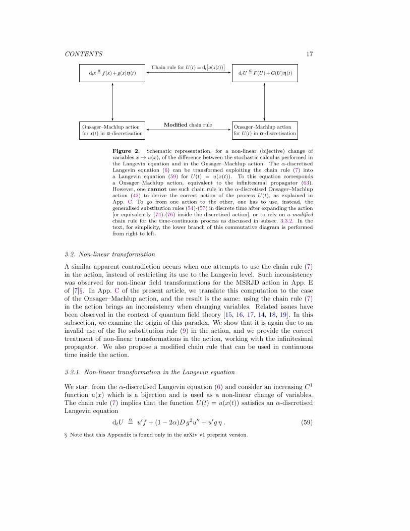
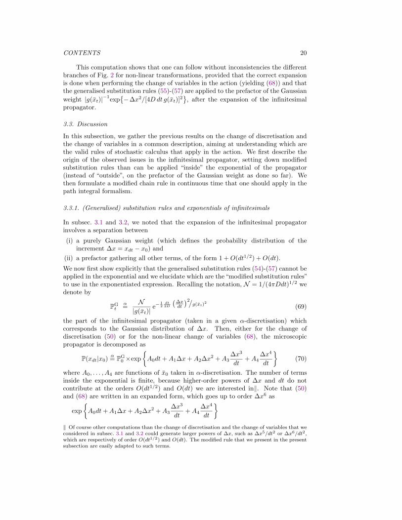

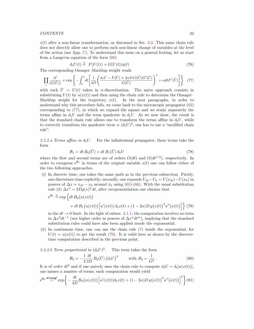


![Functional Ito calculus and stochastic integral representation of ... · Ito’s stochastic calculus [15, 16, 8, 24, 20, 28] has proven to be a powerful and useful tool in analyzing](https://static.documents.pub/doc/80x56/5edd500fad6a402d66685c11/functional-ito-calculus-and-stochastic-integral-representation-of-itoas-stochastic.jpg)


