Copyright ¤ UNU-WIDER 2004 * Both authors: World Institute for Development Economics Research, United Nations University (UNU- WIDER), Helsinki, Finland. This study has been prepared within the UNU-WIDER internship programme and research on ‘New Directions in Development Economics’. UNU-WIDER acknowledges the financial contributions to the research programme by the governments of Denmark (Royal Ministry of Foreign Affairs), Finland (Ministry for Foreign Affairs), Norway (Royal Ministry of Foreign Affairs), Sweden (Swedish International Development Cooperation Agency—Sida) and the United Kingdom (Department for International Development). ISSN 1810-2611 ISBN 92-9190-643-3 (internet version) Research Paper No. 2004/54 China’s Business Cycles Perspectives from an AD–AS Model Yin Zhang * and Guanghua Wan * August 2004 Abstract This paper represents a first attempt to study China’s business cycles using a formal analytical framework, namely, a structural VAR model. It is found that: (a) demand shocks were the dominant source of macroeconomic fluctuations, but supply shocks had gained more importance over time; (b) the driving forces of demand shocks were consumption and fixed investment in the first cycle of 1985–90, but shifted to fixed investment and world demand in the second cycle of 1991–96 and the post-1997 deflation period; and (c) macroeconomic policies did not play an important part either in initiating or counteracting cyclical fluctuations. Keywords: business cycle, structural VAR, demand shocks, supply shocks, China JEL classification: E32, O53, P24
Transcript
Copyright � UNU-WIDER 2004
* Both authors: World Institute for Development Economics Research, United Nations University (UNU-WIDER), Helsinki, Finland.
This study has been prepared within the UNU-WIDER internship programme and research on ‘NewDirections in Development Economics’.
UNU-WIDER acknowledges the financial contributions to the research programme by the governmentsof Denmark (Royal Ministry of Foreign Affairs), Finland (Ministry for Foreign Affairs), Norway (RoyalMinistry of Foreign Affairs), Sweden (Swedish International Development Cooperation Agency—Sida)and the United Kingdom (Department for International Development).
ISSN 1810-2611 ISBN 92-9190-643-3 (internet version)
Research Paper No. 2004/54
China’s Business Cycles
Perspectives from an AD–AS Model
Yin Zhang * and Guanghua Wan *
August 2004
Abstract
This paper represents a first attempt to study China’s business cycles using a formalanalytical framework, namely, a structural VAR model. It is found that: (a) demandshocks were the dominant source of macroeconomic fluctuations, but supply shocks hadgained more importance over time; (b) the driving forces of demand shocks wereconsumption and fixed investment in the first cycle of 1985–90, but shifted to fixedinvestment and world demand in the second cycle of 1991–96 and the post-1997deflation period; and (c) macroeconomic policies did not play an important part either ininitiating or counteracting cyclical fluctuations.
Keywords: business cycle, structural VAR, demand shocks, supply shocks, China
JEL classification: E32, O53, P24
The World Institute for Development Economics Research (WIDER) wasestablished by the United Nations University (UNU) as its first research andtraining centre and started work in Helsinki, Finland in 1985. The Instituteundertakes applied research and policy analysis on structural changesaffecting the developing and transitional economies, provides a forum for theadvocacy of policies leading to robust, equitable and environmentallysustainable growth, and promotes capacity strengthening and training in thefield of economic and social policy making. Work is carried out by staffresearchers and visiting scholars in Helsinki and through networks ofcollaborating scholars and institutions around the world.
UNU World Institute for Development Economics Research (UNU-WIDER)Katajanokanlaituri 6 B, 00160 Helsinki, Finland
Camera-ready typescript prepared by Adam Swallow at UNU-WIDERPrinted at UNU-WIDER, Helsinki
The views expressed in this publication are those of the author(s). Publication does not implyendorsement by the Institute or the United Nations University, nor by the programme/project sponsors, ofany of the views expressed.
1
1 Introduction
China’s economic performance in the past two decades is outstanding in two aspects:not only has it been growing faster than most developing and transition economies, ithas also steered clear of severe macroeconomic instability. Studies on the growth aspectare abundant. See, for example, Sachs and Woo (2000), Zhang and Zou (1998), Hu andKhan (1996), Borensztein and Ostry (1996) and Chow (1993). By contrast, little hasbeen published on the other aspect, namely China’s macroeconomic fluctuations orbusiness cycles which, according to Schumpeter (1939: 5), are inherent in the growthprocess.
This paper represents a first attempt to identify China’s business cycles and to explorethe characteristics and sources of the cycles. More specifically, this study examines thefluctuations in output and inflation within the aggregate-demand–aggregate-supply(AD–AS) framework. Following Blanchard and Quah (1989), the sources of thesefluctuations are attributed to two generic shocks: supply shocks that affect real outputpermanently and demand shocks whose effects on real output eventually die out. Thisgrouping of shocks helps fulfil several objectives. First, an important purpose ofbusiness cycle research is to provide advice for the formulation of counter-cyclicaldemand management policies. Real output growth and inflation are often regarded asthe most comprehensive indicators of the general state of the macroeconomy, and assuch, frequently constitute the principal concerns of policymakers. It is thus desirable toexamine what drives the movements in real output and inflation. Second, variousmacroeconomic paradigms differ, sometimes widely, in their views about howexogenous shocks are transmitted throughout the economy. Even less common groundhas been reached regarding the inner workings of developing and transition economies.The characterisation of the two shocks in this paper fits in with the AD–AS frameworkwith a vertical long-run AS curve, which is arguably a best alternative to a consensusmodel for analysing aggregate fluctuations (Blanchard, 1997; Blinder, 1997). Thisreduces the chances of obtaining biased results due to erroneous a priori assumptions.Third, China stands out among transition economies in terms of macroeconomicstability. Fischer and Sahay (2000) argue that economic performance in transitioneconomies depends importantly on both structural reforms and stabilisation policies,though initial conditions also matter. Dibooglu and Kutan (2001) show that realexchange rate movements in Poland and Hungary were driven by different shocks,owing to different macroeconomic policies pursued by the two countries. The questionthen arises whether China’s relative stability shall be associated more with its gradualistapproach to transition or with its conduct of macroeconomic policy. Since structuralreforms typically involve the supply side of the economy while stabilisation measureslargely land on the demand side, the results from our model will shed light on thisquestion.
The remainder of the paper is organised as follows. The next section introduces ourmodelling approach along with the data and issues related to model estimation.Section 3 presents empirical results. Further discussions of the findings are offered inSection 4 and Section 5 concludes.
2
2 A structural VAR of output growth and inflation
2.1 Methodology
The theoretical framework of our analysis is the textbook AD–AS model (e.g., Mankiw,2000), where the short-run equilibrium output y (expressed in logarithm) in period t canbe represented by
dttt yyy += * (1)
where y* is the log level of long-run equilibrium output and yd is the deviation of y fromits long-run value in the short-run. Assume that the long-run level of output follows anI(1) process:
* *1 1( ) s
t t ty y Lα ε−= + (2)
where εs represents supply shocks and is a white noise, the lag polynomial 1( )Lα has
absolutely summable coefficients, and all the roots of the characteristic equation of
1( )Lα lie within the unit circle.1 The short-run deviation yd is induced by demand
shocks εd:
1( )d dt ty Lβ ε= , (3)
where 1( )Lβ is a lag polynomial, similar to 1( )Lα . Combining equations (1)–(3) yields
1 1 1( ) (1 ) ( )s dt t t t ty y y L L Lα ε β ε−∆ = − = + − . (4)
Equation (4) indicates that supply shocks εs can cause permanent shifts in the outputlevel y unless 1(1) 0α = , whereas demand shocks εd merely have transitory effects.
Provided that the short-run AS curve is not horizontal, equation (1) implies a short-runPhillips curve trading off inflation and output. A common specification of the Phillipscurve augmented with supply shocks and inflation inertia is the ‘triangle model’ as perGordon (1998):
*1( ) ( )( ) ( ) s
t t t t tp L p L y y Lγ θ φ ε−∆ = ∆ + − + , (5)
where p is the general level of prices, and ( )Lγ , ( )Lθ , and ( )Lφ are again lagpolynomials. The first term on the right-hand side of equation (5) embodies inflationinertia, introduced through overlapping wage and price contracts and expectationformation. The second term is the output gap component of standard Phillips curvemodels. It measures the effect of excess demand on inflation. The addition of the thirdterm, supply shocks, conveys the idea that part of short-run fluctuations are attributable
1 All lag polynomials in this paper possess these properties unless otherwise specified. That is, the lagpolynomials describe stationary processes and are invertible.
3
to transitory adjustments from one long-run equilibrium to another. Substitutingequations (1) and (3) into equation (5) gives
2 2( ) ( )s dt t tp L Lα ε β ε∆ = + , (6)
where 12 ( ) [1 ( ) ] ( )L L L Lα γ φ−= − and 1
2 1( ) [1 ( ) ] ( ) ( )L L L L Lβ γ θ β−= − . Equation (6)
shows that neither of the two shocks have permanent effect on the level of inflation.Thus, the rate of inflation is assumed to be stationary, thought the price level could benonstationary.
The structural model, as represented by equations (4) and (6), has numerous statisticallyequivalent representations, and thus cannot be estimated directly. To recover thestructural parameters from their reduced-form counterparts, at least four independentrestrictions on the structural model are needed. Following Blanchard and Quah (1989),restrictions are imposed on the variance-covariance matrix of the structural model.Equation (4) itself implies a restriction on the long-run property of the system—thelong-run multiplier of εd on y is zero. This restriction, upon orthogonalisation andnormalisation of the structural shocks, suffices to exactly identify the system.
2.2 Data and model estimation
Our analysis focuses on the period of 1985–2000. The level of real output is representedby real gross industrial output. Although real GDP might seem a more appropriatechoice, its quarterly series is only available from 1994 onwards and is not long enoughfor the intended econometric analysis. Besides, there are grounds to argue that realindustrial production can serve as a good indicator of aggregate economic activity, andthat other broader measures may not be preferable. For one thing, agriculturalproduction, as important as it is for the Chinese economy, has strong seasonal patternsand is still under the rule of natural forces. Including agricultural output will probablyadd too much noise to the data and cloud the overall picture. For another, the level ofactivity in the service sector, which now constitutes about a third of GDP, turns on thatof the industrial sector. That the industrial sector plays a pivotal role in the course ofmacroeconomic fluctuations is true not just for countries like China where the servicesector is small relative to the industrial sector. Even in more advanced economies suchas the US, Japan, Germany, and so on, the output of the industrial sector, especially thatof the manufacturing industries, finds its way into the coincident index compiled bygovernment agencies and research institutions monitoring business cycles. The inflationrate is measured by changes in the retail price index (RPI). The alternative measure, theconsumer price index (CPI), includes prices of such services as housing, transportation,health care, and so on. For much of the sample period, these prices were administeredby the government and did not reflect market conditions.
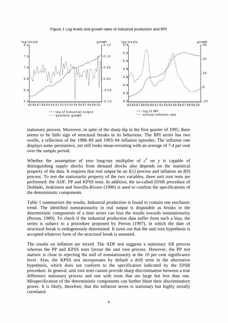
Both real gross industrial output and RPI are obtained by converting the monthly datareported in China Monthly Statistics into seasonally adjusted quarterly observations.Figure 1 shows the log levels and growth rates of both series. The level of industrialproduction clearly exhibits an upward trend. Its first difference—the quarter-to-quartergrowth rate, appears stationary and has a mean of 2.9 per cent. This suggests thatindustrial production can be characterized by either a random walk with drift or a trend
4
Figure 1 Log levels and growth rates of industrial production and RPI
stationary process. Moreover, in spite of the sharp dip in the first quarter of 1995, thereseems to be little sign of structural breaks in its behaviour. The RPI series has twoswells, a reflection of the 1988–89 and 1993–94 inflation episodes. The inflation ratedisplays some persistence, yet still looks mean-reverting with an average of 7.4 per centover the sample period.
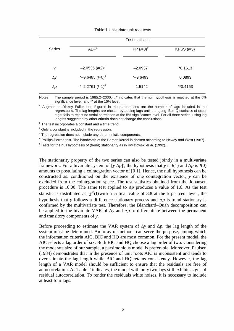
Whether the assumption of zero long-run multiplier of εd on y is capable ofdistinguishing supply shocks from demand shocks also depends on the statisticalproperty of the data. It requires that real output be an I(1) process and inflation an I(0)process. To test the stationarity property of the two variables, three unit root tests areperformed: the ADF, PP and KPSS tests. In addition, the so-called DJSR procedure ofDoldado, Jenkinson and Sosvilla-Rivero (1990) is used to confirm the specifications ofthe deterministic components.
Table 1 summarizes the results. Industrial production is found to contain one stochastictrend. The identified nonstationarity in real output is disputable as breaks in thedeterministic components of a time series can bias the results towards nonstationarity(Perron, 1989). To check if the industrial production data suffer from such a bias, theseries is subject to a procedure proposed by Perron (1997), in which the date ofstructural break is endogenously determined. It turns out that the unit root hypothesis isaccepted whatever form of the structural break is assumed.
The results on inflation are mixed. The ADF test suggests a stationary AR processwhereas the PP and KPSS tests favour the unit root process. However, the PP teststatistic is close to rejecting the null of nonstationarity at the 10 per cent significancelevel. Also, the KPSS test incorporates by default a drift term in the alternativehypothesis, which does not conform to the specification indicated by the DJSRprocedure. In general, unit root tests cannot provide sharp discrimination between a truedifference stationary process and one with roots that are large but less than one.Misspecification of the deterministic components can further blunt their discriminatorypower. It is likely, therefore, that the inflation series is stationary but highly seriallycorrelated.
5
Table 1 Univariate unit root tests
Test statistics
Series ADFa PP (l=3)e KPSS (l=3)f
y –2.0535 (l=2)b –2.0937 *0.1613
∆y *–9.6485 (l=0)c *–9.6493 0.0893
∆p *–2.2761 (l=1)d –1.5142 **0.4163
Notes: The sample period is 1985:2–2000:4. * indicates that the null hypothesis is rejected at the 5%significance level, and ** at the 10% level.
a Augmented Dickey–Fuller test. Figures in the parentheses are the number of lags included in theregressions. The lag lengths are chosen by adding lags until the Ljung–Box Q-statistics of ordereight fails to reject no serial correlation at the 5% significance level. For all three series, using laglengths suggested by other criteria does not change the conclusions.
b The test incorporates a constant and a time trend.c Only a constant is included in the regression.d The regression does not include any deterministic components.e Phillips-Perron test. The bandwidth of the Bartlett kernel is chosen according to Newey and West (1987).f Tests for the null hypothesis of (trend) stationarity as in Kwiatowski et al. (1992).
The stationarity property of the two series can also be tested jointly in a multivariateframework. For a bivariate system of [y ∆p]′, the hypothesis that y is I(1) and ∆p is I(0)amounts to postulating a cointegration vector of [0 1]. Hence, the null hypothesis can beconstructed as: conditioned on the existence of one cointegration vector, y can beexcluded from the cointegration space. The test statistics obtained from the Johansenprocedure is 10.00. The same test applied to ∆p produces a value of 1.6. As the teststatistic is distributed as )1(2χ with a critical value of 3.8 at the 5 per cent level, thehypothesis that y follows a difference stationary process and ∆p is trend stationary isconfirmed by the multivariate test. Therefore, the Blanchard–Quah decomposition canbe applied to the bivariate VAR of ∆y and ∆p to differentiate between the permanentand transitory components of y.
Before proceeding to estimate the VAR system of ∆y and ∆p, the lag length of thesystem must be determined. An array of methods can serve the purpose, among whichthe information criteria AIC, BIC and HQ are most common. For the present model, theAIC selects a lag order of six. Both BIC and HQ choose a lag order of two. Consideringthe moderate size of our sample, a parsimonious model is preferable. Moreover, Paulsen(1984) demonstrates that in the presence of unit roots AIC is inconsistent and tends tooverestimate the lag length while BIC and HQ retains consistency. However, the laglength of a VAR model should be sufficient to ensure that the residuals are free ofautocorrelation. As Table 2 indicates, the model with only two lags still exhibits signs ofresidual autocorrelation. To render the residuals white noises, it is necessary to includeat least four lags.
6
Table 2 Diagnostic statistics for different lag lengths (p-values in parentheses)
Notes: Q(12): Ljung–Box test statistics for no autocorrelation of order 12, distributed as 2 (8)χ .
Portmanteau: multivariate test for no autocorrelation, distributed as 2 (40)χ . JB: Jarque–Bera
test for normality, distributed as 2 (2)χ . Normality: multivariate test for normality, distributed as2 (4)χ . AIC: Akaike information criterion; BIC: Baynesian information criterion; HQ: Hannan–
Qinn criterion.
The normality tests reject the null for all lag lengths listed in Table 2. The two inflationspurts in 1988–89 and 1993–94 and the sharp decline in industrial production in the firstquarter of 1995 are largely responsible for the violation of normality. Although it ispossible to alleviate the problem by incorporating dummy variables for these incidents,this option is not taken up here. The three occurrences are caused by unusually large
7
demand and/or supply shocks, yet the nature of these shocks is no different from that ofother shocks. Non-normality will not distort the point estimates of impulse responsesand variance decomposition, though it does affect their interval estimates.
3 Estimation results
Based on the above discussions, a bivariate VAR(4) model of ∆y and ∆p is estimated.Parameter estimates of the reduced-form model are not reported as they are noteconomically interpretable. Attention is focused on innovation accounting of thestructural model.
3.1 The dynamics of real output and inflation
Graphed in Figure 2 are the impulse response functions that trace out the impact on thelevels of output and inflation of supply and demand shocks. The left panel displays theresponses of output. It shows that one unit (i.e., one standard deviation) positive supplyshock raises output by about 1.4 per cent in the long run. The adjustment is completedwithin three to four years. A typical demand shock has strong impact effects on output,increasing it by up to 1.6 per cent in the first three quarters. This demand-led expansionlasts about two and a half years, and output eventually returns to its original level afterabout five years.
The dynamics of the inflation rate is demonstrated in the right panel of Figure 2. Asexpected, a positive supply shock causes a slight dip in inflation, while a positivedemand shock leads to a sharp increase in inflation. The inflationary effects of thedemand shock persist for about two and a half years, followed by a period of over-adjustment (i.e., deflation). The whole process takes about five to six years to complete.
Figure 2 Impulse responses of industrial production and RPI inflation
-0.5
0.0
0.5
1.0
1.5
2.0
5 10 15 20 25 30 35 40Supply shock Demand shock
-1
0
1
2
3
4
5 10 15 20 25 30 35 40
Industrial production RPI inflationper cent per cent
8
Several observations follow from the above description. First, the impulse responses ofoutput and inflation are consistent with the predictions of the AD–AS model. A positivesupply shock raises output and lowers inflation. In contrast, a positive demand shockinduces increases in both output and inflation. Second, output responds strongly to bothshocks while inflation does not seem to be sensitive to supply shocks. Third, the speedof adjusting to equilibrium differs slightly for the two shocks. In the case of supplyshocks, the transition from the old equilibrium to the new one attains in four to fiveyears. For demand shocks, it takes up to six years to restore the original equilibrium. Onthe basis of these results, the average business cycle will last between four to six years.Finally, the responses of both series to a demand shock indicate a positive correlationbetween output and inflation in the short run—one of the many versions of the Phillipscurve.
Price liberalisation and the legacy of a monetary overhang made disinflation anindispensable part of macroeconomic stabilisation in transition economies, especially inthe early stages of transition. Disinflation carries real cost. A widely-used measure ofthat cost is the ‘sacrifice ratio’, which is defined as the percentage decrease in industrialproduction required to reduce the inflation rate by one percentage point. This can beapproximated by the ratio of the cumulative effects of a demand shock on output tothose on inflation rate, calculated over the average length of the business cycle—24quarters. The calculation results in a value of 0.61, which suggests that the cost of onepercentage point reduction in inflation is about a 0.6 per cent decrease in output. Hence,the strong procyclical behaviour of the inflation rate is attributable to the sensitivity ofinflation to demand shocks. The presence of supply shocks will attenuate the positiverelation between inflation and output, especially if the contributions to aggregatefluctuations of supply shocks are more important than those of demand shocks. Therelative importance of the two shocks is the question to which we now turn.
3.2 The relative importance of supply and demand shocks
To gauge the relative importance of supply and demand shocks for explaining thefluctuations in real output and inflation, two types of decompositions are conducted—forecast error variance decomposition (FEVD) and historical decomposition (HD).
The first calculates the share of the total forecast error variance of inflation or outputthat is due to a particular shock at various horizons. It provides an assessment of theaverage contributions by the two types of shock over the sample period. Table 3tabulates the FEVD results. The first point to notice is that demand shocks account forover 90 per cent of the variability of the inflation rate at all forecast horizons. In themedium to long run, the share of demand shocks increases to 98 per cent. Suchsupremacy implies that, so far as the fluctuations of inflation are concerned, the role ofsupply shocks is minimal. Demand shocks are also important in driving cyclicalfluctuations in real output. They explain about 40 per cent of output variationsthroughout the first year. Over the two- to five-year horizons, demand shocks accountfor 20 to 30 per cent of output variability. These results are in agreement with thefindings from the impulse response analysis discussed earlier.
9
Table 3 Forecast error variance decomposition
Industrial production RPI inflationHorizon
(Quarters) Supplyshock
Demandshock s.e. Supply shock
Demandshock s.e.
1 55.5 44.5 41.5 9.7 90.3 25.2
2 57.3 42.7 33.3 9.4 90.6 14.0
3 53.8 46.2 15.5 5.5 94.5 9.9
4 61.4 38.6 10.2 3.5 96.5 1.2
8 73.2 26.8 12.0 1.9 98.1 4.3
12 77.9 22.1 11.5 1.9 98.1 4.4
16 80.7 19.3 10.4 1.9 98.1 4.8
20 82.9 17.1 9.8 1.9 98.1 4.9
40 89.4 10.6 7.4 1.9 98.1 4.8
60 92.4 7.6 5.9 1.9 98.1 4.8
Notes: Impulse responses are entered in percentage points. The standard errors (s.e.) are asymptoticvalues calculated as per Warne (1993).
The importance of demand shocks as suggested by the FEVD invites a furtherquestion—whether this is the case for every episode of the sample period. In otherwords, how representative is the average result of individual episodes, and have therebeen any changes in the characteristics of the underlying shocks? To answer thesequestions, it is instructive to distil the demand components of the two series, whichrepresent the part of each series due to demand shocks from the third quarter of 1986onwards. These are plotted in Figure 3 along with the cyclical components of the twoseries obtained by applying the Hodrick–Prescott (HP) filter to the original series.2The HP filter isolates from a time series those components within a preset range offrequencies, which in this case has been set to 2 to 32 quarters. Consequently, theextracted cyclical component encompasses short-run fluctuations caused by demandshocks as well as supply shocks. The differences between the demand component of aseries and its HP cyclical component shall then reflect the fluctuations caused by supplyshocks at business cycle frequencies.
2 The smoothing parameter λ of the HP filter is set to 1600. Supposedly, other high frequencycomponents—seasonal and irregular variation—have been removed by the X-11 procedure.
10
Figure 3 Demand and cyclical components of industrial production and RPI inflation
Industrial production RPI inflationper cent per cent
In both panels of Figure 3, the turning points of the demand components match closelythe turning points of the HP cyclical components, attesting to the importance of demandshocks as a source of business cycle fluctuations. The relations between the demandcomponents and their corresponding HP cycles have not been invariable. With respectto output, the demand component is slightly lower than the HP cycle before the firstquarter of 1988. Starting from the second half of 1988, the HP cycle becomes lowerthan the demand component, and the discrepancy widened in 1990–91. However, thegap is closed up quickly by the sharp rises of the HP cycle from the third quarter of1992 through 1993. From the end of 1996, the HP cycle is again above the demandcomponent and the divergence grows wider in the last three years of the sample. For theinflation rate, the HP cycle increases faster than the demand component in 1988,eliminating the initial difference between the two. A dip of the HP cycle in the thirdquarter of 1992 sets apart the two time paths once more. After a period of convergencein 1995 and 1996, they start to depart from each other again, more notably so from1998. These relative movements of the demand components and the cyclicalcomponents point to the presence of important supply shocks in 1988–89, 1992–93 andaround 1998.
Figure 4 plots the four-term moving averages of the structural shocks recovered fromthe residuals of the estimated VAR model.3 In the left panel, large negative supplyshocks are found during 1988–89. Strong positive supply shocks appeared in 1992–93.According to the impulse responses in Figure 2, a positive supply shock reducesinflation, and brings about a permanent increase in the level of real output. A negative
3 It is not appropriate to use the derived structural shocks directly. The derived shocks are white noisesby construction. However, quarterly data are themselves average observations on the underlying datagenerating processes which may be of higher frequencies. The true structural shocks sampled on aquarterly basis will thus be serially correlated. Applying four-term moving average to the derivedshocks is a convenient, though not the only, way to render the shocks more interpretable.
11
Figure 4 Historical realisations of supply and demand shocks
-1.5
-1.0
-0.5
0.0
0.5
1.0
1.5
88 90 92 94 96 98 00-1.5
-1.0
-0.5
0.0
0.5
1.0
1.5
88 90 92 94 96 98 00
supply shocks demand shocks
supply shock does the opposite. It can be then deduced that the negative supply shocksoccurring in 1988–89 should have reinforced the effect of positive demand shocks oninflation, but have partly offset the effect of demand shocks on industrial production. Asthe HP cycle does not discriminate between permanent shocks and transitory shocks, theHP cycle of output is lower than the corresponding demand component whereas the HPcycle of inflation rises faster the demand component.
The situation in 1992–93 can be explained analogously. Less amenable to thisinterpretation is the period of 1998–99. Figure 4 suggests that there could have appearedsome minor negative supply shocks around this time. In Figure 3, the HP cycle of theinflation rate moves accordingly further above the demand component. However, thesupply shocks do not seem to present themselves in the HP cycle of output, whichcontinues to exceed the demand component by the same amount as it does before theshocks take place. Two tentative explanations can be offered for the behaviour ofoutput. First, the problem may lie with the algorithm of the HP filter. The positivesupply shocks in 1992–93 should have raised the long-run trend of output permanently.Because of the limited sample size, the increases in the long-run trend are notadequately reflected in the trend estimated by the HP filter. Also, the HP filter has beenshown to have poor end-of-sample properties (Rennison, 2003). This means theestimated deviations from the trend will be greater than their true values. Second, it maytake some time for the effects of the large positive supply shocks in 1992–93, coupledwith the small ones in 1994 and late 1996 to early 1997, to reach their full potential.That is, the cyclical component of output is not only the result of contemporaneousshocks, but is also under the influence of shocks from previous periods.
The time plots of historical supply and demand shocks also provide an account of howthe forces driving inflation and output have evolved. The years before 1995 arecharacterised by strong shocks, both from the demand side and from the supply side,and both positive and negative. Since 1995 the magnitudes of shocks have dampenedsubstantially. The first half of the 1990s stands out as an episode of expansionary supplyand demand shocks. In comparison, the late 1980s experienced expansionary demandshocks but contractionary supply shocks.
12
4 How does the model interpret China’s business cycles?
The supply and demand shocks as conceptualized by equations (4) and (6) are each acomposite of disturbances deriving from different sources. This section examines howthe results can help explain China’s business cycles in the sample period.
4.1 The chronology of China’s business cycles
There exists, as at the time of writing, no official chronology of China’s business cycles.Partly this is due to the lack of data for compiling such a chronology. The commonly-used rule of thumb—that a downturn consists of at least two consecutive quarters ofnegative GDP growth—apparently does not apply as post-reform China has notexperienced negative GDP growth.
Previous studies on China’s macroeconomic cycles either sidestepped this question orproposed a division of cycles based on the rates of annual inflation and/or GDP growthrates. Examples of the latter include:
iii) Liu (2000): 1977–81, 1981–86, 1987–90, 1991–.
The demand components of output and inflation in Figure 3 suggest a demarcation ofthe cycles as follows: 1985/86–90, 1991–96, and 1997–. This is largely consistent withYu (1997), Oppers (1997) and Liu (2000). However, two major differences must benoted. First, the years 1985–86 are included in the cycle ending in 1990 and the yearsafter 1997 are assigned to another cycle. Amalgamating 1985 and 1986 into the 1987–90 cycle is not merely out of consideration for convenience as our data set starts with1985. It is also justified on the ground that the contraction from late 1985 to early 1986was mild, short-lived and limited in scope. By the second quarter of 1986, the economywas well on its way to rebound. Indeed, Oppers (1997) observed that the years between1984 and 1989 can be treated as one cycle. The demand components exhibit muchdiminished cyclicality after 1997, suggesting systematically different behaviour. Thecited researches fail to explore this point perhaps because they employed data up to1998. Our analysis based on more recent information indicates that 1997 marks thebeginning not only of another cycle but also of a new phase of China’s macroeconomicfluctuations. Moreover, the impulse response analysis shows that it takes four to sixyears for the effects of supply and demand shocks to dissipate. The average duration ofa cycle found by examining the demand components—five to six years—corroboratesthe previous result. Note also that the ups and downs of the demand components accordwell with the HP filter detrended series. Since the HP filter used here extracts timeseries components of periodicity less than or equal to eight years, the conformancefurther demonstrates the predominance of demand shocks as the sources of China’sbusiness cycles.
Hence, in a stretch of sixteen years between 1985 and 2000, China experienced twocomplete cycles and one that is currently underway. The cyclical behaviour of theeconomy appears to have undergone two distinct phases. The first phase, from 1985 to1996, contained two cycles with intensifying inflation fluctuations and large oscillations
13
in real activity. The second phase of 1997–2000 was characterised by flat growth anddisconcerting deflation.
4.2 Sources of demand shocks
The importance of demand shocks indicated by the results in section 3 does not presentmuch of a surprise. After all, some legacies of the centrally-planned system, such aswidespread ‘soft-budget constraint’, cannot be eliminated overnight. As Kornai (1980)observes, the prevalence of soft-budget constraint can put the economy under constantpressure to over-expand. Meanwhile, economic reform has led to rapidly rising personalincome, easier access to the world market and more (legal or illegal) profitableinvestment opportunities, which may also give rise to overheating. The questionremains, however, as to what really underlay demand pressures in this period, or, inother words, how the demand components as shown in Figure 3 can be traced tomovements in the prominent ingredients of aggregate demand.
A relatively straightforward way towards this end is to examine the correlationsbetween the demand components and the prime suspects of demand pressures—excesses in fixed investment, consumption and export. This amounts to conductingsimple regressions of the former on the deviations from the trend, or the cyclicalcomponents, of the latter across different periods. Derived through HP filtering, thecyclical components of fixed investment, retail sales (as a proxy for privateconsumption), and exports are plotted in Figure 5. The regression results are presentedin Table 4.
Figure 5 HP-detrended cyclical components of fixed investment, retail sales and exports
With regard to industrial production, the regressions show that fixed investment issignificant in equations for the second cycle and the whole sample, but not for thedeflation period. It also appears important in the equation for the first cycle, albeit witha puzzling negative sign. Retail sales play a significant role in the first cycle while theinfluence of exports dominates in the deflation period of 1997–2000. Quite similarresults occur with the inflation equations, except that the export series is significant inthe regressions for the entire period and for the last two sub-periods. Another point tonote is that, with the exception of the first cycle, the R2s of the inflation equations arehigher than those of the industrial production equations. This signifies that the demandcomponent of inflation has a stronger correlation with the excesses and slumps in fixedinvestment, retail sales and exports. To the extent that causality runs from the threevariables to inflation, this piece of evidence confirms, once again, that demand shocksare the foremost force behind the movements of inflation.
The above findings are in line with the indications of Figure 5. The upswing of the firstcycle (1986–90) was brought about by excessive expansion in both investment andretail sales. During this period, state-owned enterprise (SOE) reforms, fiscaldecentralisation and easy bank credit fuelled high wage growth and rapid expansion infixed investment. Price reform raised expected inflation rates. When the governmentattempted to cool off the economy by tightening credit quotas and imposingadministrative controls, both investment and retail sales plummeted.
This pattern of double-expansion and double-dip in investment and consumptionchanged substantially in 1991–2000. Retail sales in Figure 5 displayed stabilitythroughout the period, reflecting a subdued role of consumption in generating cyclicalfluctuations. The expansion phase of the second cycle was driven by the investmentboom of 1992–93. Fixed investment also managed a mild turnaround between 1998 and1999, thanks to large government outlays on infrastructure investment. Exports assumeda higher profile in this period. Strong exports growth occurred in 1994, which may haveprolonged the upswing of the second cycle and undermined the government’s effort tocontain excess demand pressure. Negative shocks to exports in 1998, in contrast, mighthave contributed to deflation.
To sum up, demand shocks in the first cycle are largely attributable to consumption andfixed investment, whilst in the later years they are more closely associated with fixedinvestment and exports. A number of factors could have contributed to these variationsfrom the first cycle to the later two periods. First of all, household expectations aboutinflation and uncertainty of future income and expenditure have changed, partly due topast experience and partly in response to reforms in employment, education and healthcare systems. On the one hand, the inflation episodes in 1985–86 and 1988–89 helpedhouseholds eventually break away from the psychology moulded in the central planningera when price stability and shortage were the norm. Certainly, expectations of futureinflation would still raise current consumption, but blind stockpiling had become afading bygone. On the other hand, a growing number of SOE employees were laid offor became de facto unemployed especially in the latter half of the 1990s, amidstacceleration in dismantling the old welfare system in the urban areas. Increaseduncertainty about the future propels risk-averse households to build up a buffer stock ofsavings (Carroll, 1992; Zhang and Wan, 2002). Added to this uncertainty is theenlarging income disparity between the coastal and the inland regions, between citiesand the countryside, and among different professions and social groups. All thesefactors combined make consumption growth fall behind output growth. As such, the
16
reduced volatility of consumption in the later periods not only indicates consumptionsmoothing, but also signals weaker consumption demand.
The second cycle coincides with yet another reform cycle. The renewed momentum ofreform, following Deng Xiaoping’s tour of south China, touched off an investmentboom in 1992–93. This was further facilitated by rapidly accumulating householdsavings, devolution to local governments of the power to ratify investment projects, anda proliferation of financing conduits other than bank lending. An upswing driven byfixed investment, albeit eventually bringing in its train rises in consumption demand andhikes in consumer goods prices, entails a downturn different from one ensuing on aconsumption-led expansion. Because investment projects take time to complete andbring forth new capacity, the downturn will be more protracted than the time requiredfor simply liquidating excess inventories.
Macroeconomic management in the second cycle leaned more towards market-orientedlevers, too. To avert the undue hardship caused by indiscriminate administrativerestraints, measures like interest rates adjustment and treasury bonds were activelyutilized. The focus of administrative controls was placed on maintaining order infinancial markets by cracking down on ‘illegal’ fund raising schemes, bank lending tonon-bank financial institutions, and so on. Traditional tools of tightening credit quotas,reducing ratified investment projects and price surveillance were also involved, yet in amore selective and flexible manner. As can be expected of these changes, the trough ofindustrial growth became shallower whereas the petering out of inflation spouts grewmore drawn out.
The foreign sector assumed a high profile in the second and third cycles, due to thesurge of inward foreign direct investment (FDI) and the success of export promotion. In1992–96, FDI increased by leaps and bounds. The annual inflows reached US$41.73billion in 1996, nearly ten folds of the US$4.37 billion in 1991 (SYC, 1999). The shareof FDI in total domestic fixed investment rose from 4 per cent or so in 1991 to over 17per cent in 1993 and 1994. The ratio declined a little in the following years, but stillremained above 13 per cent.4 A large proportion of these investments went into export-oriented manufacturing industries. In the meantime, a series of foreign exchangereforms5 and fiscal incentives (tax rebates) were implemented to stimulate exportgrowth. As a result, exports not only multiplied in terms of absolute volume, but alsoincreased its share in GDP. Particularly noteworthy is the 1994 exchange rate reformthat unified the official exchange rate with the swap market rate, and led to a moreflexibly managed exchange rate regime. In the same year, China’s exports expanded by32 per cent, followed by another 23 per cent increase in 1995 (SYC, 2000). Although itis debatable as to how much of this rapid export expansion can be ascribed to thedevaluation of the official exchange rate, the increase in itself proved to be not welltimed. It came at a time when the annual inflation rate (as measured by percentage
4 These ratios are calculated using FDI data from SYC (1999) and fixed investment data from WDI(2000).
5 The Chinese currency Renminbin (RMB) underwent substantial devaluation between 1990 and 1994,from 4.78 yuan to the US dollar to 8.62 yuan. Convertibility on current account was established in1996.
17
growth of CPI) hit a record high of 24.1 per cent (SYC, 2000), thus complicated the taskof containing excess demand pressure.
The Asian financial crisis constituted a major negative external shock. Although thecontagion of exchange rate collapse and large-scale capital flight did not spread acrossChina’s borders, exports dived sharply in 1998 and in the first half of 1999. Meanwhile,FDI inflows stalled in 1998 and then declined in 1999. After monetary easing failed tofend off the deflation that set in 1998, fiscal policy, largely dormant for years, wasbrought back into action. However, pump-priming via public investment ininfrastructure did not instigate an instant and strong upturn in non-state investment.Private consumption remained stable, yet flat. It seems therefore that the external sectorheld sway in the deflation period.
4.3 Potential output and supply shocks
The Blanchard–Quah decomposition employed in this study derives from the notion of avertical long-run Phillips curve. The historical decomposition of output can thereby beused to construct a measure of potential output.
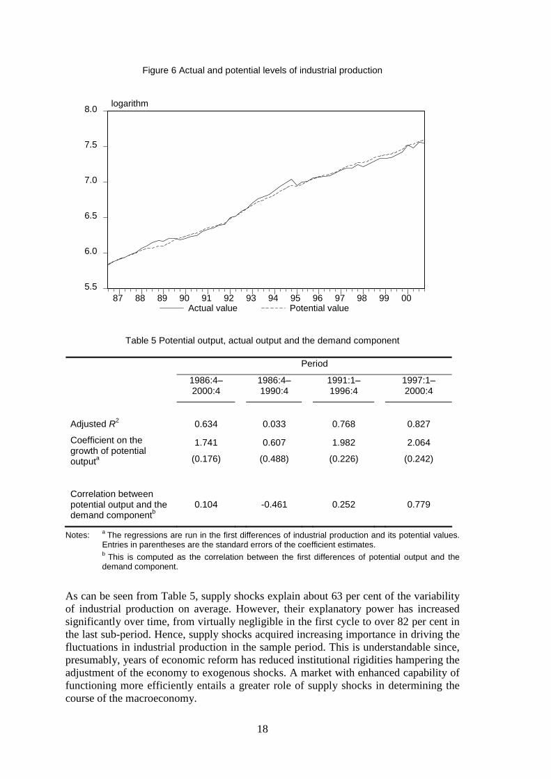
Theoretically, potential output corresponds to the level of output that obtains when alladjustments arising from nominal rigidities and misperception have completed. Withinthe context of the structural VAR model of equations (4) and (6), this definition ofpotential output can be identified with the permanent component of industrialproduction. It is the time path of industrial production in the absence of demand shocks.The computed potential level of industrial production is shown in Figure 6, along withits observed values. The differences between the two series represent the output gaps—percentage deviations of actual output from its potential value. During the two inflationepisodes (1988–89 and 1993–94), positive output gaps (excess of actual output overpotential output) reached as high as 10 per cent (in the fourth quarter of 1988) and 12per cent (in the fourth quarter of 1994) respectively. This demonstrates that short-runsupply is rather elastic, perhaps a reflection of widespread underemployment of labourin the SOEs and a very fluid population of rural migrant workers.
At first glance, actual output in Figure 6 seems to track potential output well despitedeviations occurring from time to time. This does not necessarily constitute evidencethat supply shocks explain the bulk of output fluctuations. A high correlation betweenthe levels of two I(1) series may come about in the presence of a dominant drift term,even if the two series are not genuinely related in any way. The forecast error variancedecomposition of section 3 suggests that demand shocks are very important inaccounting for the business cycle frequency movements of industrial production. Thatresult, however, is based on the assumption that supply and demand shocks are of fixedsizes. As is evident in Figure 4, the magnitudes of both types of shocks have variedsubstantially over time. To reveal the role of supply shocks in different historicalperiods, simple regressions have been conducted to regress the first differences of actualoutput on the first differences of potential output. Table 5 reports the results for theentire sample and the three sub-periods.
18
Figure 6 Actual and potential levels of industrial production
5.5
6.0
6.5
7.0
7.5
8.0
87 88 89 90 91 92 93 94 95 96 97 98 99 00Actual value Potential value
logarithm
Table 5 Potential output, actual output and the demand component
Period
1986:4–2000:4
1986:4–1990:4
1991:1–1996:4
1997:1–2000:4
Adjusted R2 0.634 0.033 0.768 0.827
Coefficient on thegrowth of potentialoutputa
1.741
(0.176)
0.607
(0.488)
1.982
(0.226)
2.064
(0.242)
Correlation betweenpotential output and thedemand componentb
0.104 -0.461 0.252 0.779
Notes: a The regressions are run in the first differences of industrial production and its potential values.Entries in parentheses are the standard errors of the coefficient estimates.b This is computed as the correlation between the first differences of potential output and thedemand component.
As can be seen from Table 5, supply shocks explain about 63 per cent of the variabilityof industrial production on average. However, their explanatory power has increasedsignificantly over time, from virtually negligible in the first cycle to over 82 per cent inthe last sub-period. Hence, supply shocks acquired increasing importance in driving thefluctuations in industrial production in the sample period. This is understandable since,presumably, years of economic reform has reduced institutional rigidities hampering theadjustment of the economy to exogenous shocks. A market with enhanced capability offunctioning more efficiently entails a greater role of supply shocks in determining thecourse of the macroeconomy.
19
What then are the possible sources of supply shocks? First, China has accumulated amassive pool of migrant rural labourers in the reform period. The process of rural-to-urban, agriculture-to-non-agriculture labour transfers accelerated in later years, but wasnever smooth. From time to time, there were eruptions of regional protectionism andcrackdowns on ‘illegal’ migrant workers. The disturbances, both positive and negative,to the supply of industrial labour force are not well reflected in the official employmentstatistics, but can nevertheless be of a significant magnitude. Second, increases in thevolumes and volatility of international trade and FDI inflows can result in supply shocksvia their impact on domestic investment, resource allocation and technological progress.Third, the government, by tightening or easing credit controls, can shift the allocation ofresources between the state and non-state sectors, which in turn affects the economy-wide level of productivity as the non-state sector is generally more efficient (Brandt andZhu, 2000, 2001).
The derived potential output also casts some light on the effectiveness of demandmanagement policy. The last row of Table 5 presents the correlations between thepermanent and transitory components of real output over different periods. As discussedabove, movements in potential output are caused by supply shocks while the transitorycomponent represents the cumulated effects of demand shocks. If macroeconomicpolicy is the prime mover of demand shocks, the degree of co-variation between the twocomponents of output can be regarded as signifying how accommodatingmacroeconomic policy was in the specified period. Should this be true, the figures inTable 5 would suggest that policy was counteractive to supply shocks in the first cycle,but has grown much more accommodating in the later years. More specifically, it can beinferred from the description that when faced with negative supply shocks in 1988–89and 1998–99, the government pursued expansionary policies in the first case, yetimplemented restrictive policies in the second occasion. These scenarios are clearly atodds with the officially announced policy intentions. Neither are they the likelyoutcomes of implemented policies, albeit unexpected side-effects and events could havedislodged the original policy objectives. Therefore, we choose to interpret thecorrelations in Table 5 as testimony that demand management policies did not, at leastnot always, wield material influence on aggregate demand.
5 Conclusion
Based on a structural VAR model of real output and inflation, this paper analyses twotypes of exogenous shocks driving business cycles in China: demand shocks and supplyshocks. The dynamic effects, relative importance and possible origins of these shocksare explored in relation to their historical evolution.
Three interesting findings emerge. First of all, both impulse response analysis andforecast error variance decomposition show that demand shocks exerted strongerinfluence on output and inflation than do supply shocks. However, there were variationsfrom one period to another. These variations manifested themselves in a number ofways. The amplitudes of both shocks exhibited a tendency to moderate through time.Further, supply shocks have acquired more importance in the later years of the sample.Meanwhile, the major sources of demand shocks have been shifting.
20
Second, the Chinese economy is found to be experiencing another cycle started in 1997after completing two cycles: 1985–90 and 1991–96. The first cycle was dominated byconsumption and fixed investment shocks. In the second cycle and the post-1997deflation period, shocks from fixed investment and world demand occupied the centralstage. Overexpansion of investment led to slumps in private investment thereafter,leaving exports the chief engine of growth in 1997–2000.
An examination of the derived potential output gives rise to the third finding—demandmanagement policies do not seem to have been a particularly important source ofaggregate demand shocks, neither have they demonstrated effectiveness in restrainingexcess demand. Thus, stabilisation policy is not the major source of macroeconomicfluctuations, despite the close association between demand shocks and business cycles.In comparison with the evidence for other transition economies presented in Fischer andSahay (2000) and Dibooglu and Kutan (2001), greater macroeconomic stability in Chinais attributable both to its transition strategy, which moderated the impact of structuralreforms, and to non-restrictive macroeconomic policy.
References
Blanchard, O. J. (1997). ‘Is there a core of usable macroeconomics?’ AmericanEconomic Review, 87: 244-6.
—— and Quah, D. (1989). ‘The dynamic effects of aggregate demand and supplydisturbances’, American Economic Review, 79: 655-73.
Blinder, A. S. (1997). ‘Is there a core of practical macroeconomics that we should allbelieve?’ American Economic Review, 87: 240-3.
Borensztein, E. and Ostry, J. D. (1996). ‘Accounting for China’s growth performance’,American Economic Review, 86: 224-28.
Brandt, L. and Zhu, X. (2000). ‘Redistribution in a decentralized economy: growth andinflation in China under reform’, Journal of Political Economy, 108: 422-39.
—— and —— (2001). ‘Soft budget constraint and inflation cycles: a positive model ofthe macro-dynamics in China during transition’, Journal of Development Economics,64: 437-57.
Carroll, C. D. (1992). ‘The buffer-stock theory of saving: some macroeconomicevidence’, Brookings Papers on Economic Activity, 2: 61-156.
Chow, G. C. (1993). ‘Capital formation and economic growth in China’, QuarterlyJournal of Economics, 108: 809-42.
Dibooglu, S. and Kutan, A. M. (2001). ‘Source of real exchange rate fluctuations intransition economies: the case of Poland and Hungary’, Journal of ComparativeEconomics, 29: 257-75.
Doldado, J., Jenkinson, T. and Sosvilla-Rivero, S. (1990). ‘Cointegration and unitroots’, Journal of Economic Surveys, 4: 249-73.
Fischer, S., and Sahay, R. (2000). ‘The transition economies after ten years’, NBERWorking Papers No. 7664, National Bureau of Economic Research: Cambridge, MA.
21
Gordon, R. J. (1998). ‘Foundations of the goldilocks economy: supply shocks and thetime-varying NAIRU’, Brookings Papers on Economic Activity, 2: 297-333.
Hu, Z. L. and Khan, M. S. (1996). ‘Why is China growing so fast?’ IMF Staff Papers,44: 103-31. International Monetary Fund: Washington, DC.
Kornai, J. (1980). Economics of Shortage. Amsterdam: North-Holland.
Kwiatkowski, D., Phillips, P. C. B., Schmidt, P. and Shin, Y. (1992). ‘Testing the nullhypothesis of stationarity against the alternative of a unit root’, Journal ofEconometrics, 54: 159-78.
Liu, S. C. (2000). Lun zhongguo jingji zengzhang yu bodong de xin taishi (On the newtrends in China’s economic growth and fluctuations), available athttp://unionforum.cei.gov.cn/cass/report/hgjj_casrep_2000041802.htm (21 October2000).
Mankiw, N. G. (2000). Macroeconomics, 4th edn, Worth: New York.
Newey, W. and West, K. (1987). ‘A simple, positive semi-definite, heteroskedasticityand autocorrelation consistent matrix’, Econometrica, 55: 703-8.
Oppers, S. E. (1997). ‘Macroeconomic cycles in China’, IMF Working Paper No.97/135, International Monetary Fund, Washington DC.
Paulsen, J. (1984). ‘Order determination of multivariate autoregressive time series withunit roots’, Journal of Time Series Analysis, 5: 115-27.
Perron, P. (1989). ‘The great crash, the oil price shock, and the unit root hypothesis’,Econometrica, 57: 1361-401.
—— (1997). ‘Further evidence on breaking trend functions in macroeconomicvariables’, Journal of Econometrics, 80: 355-85.
Rennison, A. (2003). Comparing alternative output-gap estimators: A Monte Carloapproach. Bank of Canada Working Paper 2003-8, Ottawa, Ontario.
Sachs, J. D. and Woo, W. T. (2000). ‘Understanding China's economic performance’,Journal of Policy Reform, 4: 1-50.
Schumpeter, J. A. (1939). Business Cycles: A Theoretical, Historical and StatisticalAnanlysis of the Capitalist Process, McGraw-Hill: New York.
Statistical Yearbook of China (SYC) (1999). National Bureau of Statistics: Beijing.
—— (2000). National Bureau of Statistics: Beijing.
Warne, A. (1993). ‘A common trends model: identification, estimation and inference’,Seminar Paper No. 555, IIES, Stockholm University, Stockholm.
World Development Indicators (WDI) (2001). World Bank: Washington DC.
Yu, Q. (1997). ‘Economic fluctuation, macro control, and monetary policy in thetransitional Chinese economy’, Journal of Comparative Economics, 25: 180-95.
Zhang, Y. and Wan, G. H. (2002). ‘Household consumption and monetary policy inChina’, China Economic Review, 13: 27-52.
Zhang, T. and Zou, H. F. (1998). ‘Fiscal decentralization, public spending, andeconomic growth in China’, Journal of Public Economics, 67: 221-40.