2 (13) Introduction to Exchange Rates and the Foreign Exchange Market 1. Discovering Data Not all pegs are created equal! In this question you will explore trends in exchange rates. Go to the St. Louis Federal Reserve’s Economic Data (FRED) website at https://research.stlouisfed.org/fred2/ and download the daily United States exchange rates with Venezuela, India, and Hong Kong from 1990 to present. These can be found most easily by searching for the country names and “daily exchange rate.” a. Plot the Indian rupee to U.S. dollar exchange rate over this period. For what years does the rupee appear to be pegged to the dollar? Does this peg break? If so, how many times? Answer: The rupee appears to be pegged to the U.S. dollar at various rates from 1991 until about 1998 with intermittent volatility at places the peg appears to break. There are four distinct rates at which this peg remains, the longest of which lasting over two years from 1993 until mid 1995. b. How would you characterize the relationship between the rupee and the dollar from 1998–2008? Does it appear to be fixed, crawling, or floating during this period? How would you characterize it from 2008 onward? Answer: Over this period the exchange rate appears to be a crawling peg. Although this crawl is relatively flat for a few years at the beginning of this period, it appears free to move. However, the lack of short-term volatility suggests that the exchange rate is still being controlled and is hence crawling. From 2008 onward this appears to be a freely floating currency. The line becomes more erratic with a greater deal of short-term volatility. c. The Hong Kong dollar has maintained its peg with the United States dollar since 1983. Over the course of the period that you have downloaded what are the highest and lowest values for this exchange rate? 0.0000 10.0000 20.0000 30.0000 40.0000 50.0000 60.0000 70.0000 80.0000 1990-01-02 1991-01-02 1992-01-02 1993-01-02 1994-01-02 1995-01-02 1996-01-02 1997-01-02 1998-01-02 1999-01-02 2000-01-02 2001-01-02 2002-01-02 2003-01-02 2004-01-02 2005-01-02 2006-01-02 2007-01-02 2008-01-02 2009-01-02 2010-01-02 2011-01-02 2012-01-02 2013-01-02 2014-01-02 2015-01-02 2016-01-02 Rupee/Dollar Exchange Rate International Macroeconomics 4th Edition Feenstra Solutions Manual Full Download: https://testbanklive.com/download/international-macroeconomics-4th-edition-feenstra-solutions-manual/ Full download all chapters instantly please go to Solutions Manual, Test Bank site: testbanklive.com
Transcript
2 (13) Introduction to Exchange Rates and the Foreign Exchange Market 1. Discovering Data Not all pegs are created equal! In this question you will explore trends in exchange rates. Go to the St. Louis Federal Reserve’s Economic Data (FRED) website at https://research.stlouisfed.org/fred2/ and download the daily United States exchange rates with Venezuela, India, and Hong Kong from 1990 to present. These can be found most easily by searching for the country names and “daily exchange rate.”
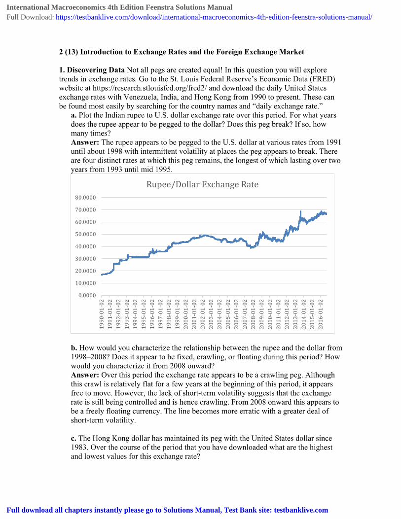
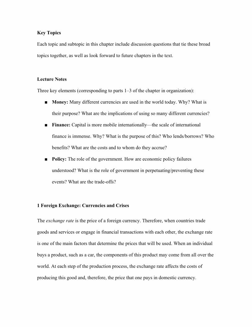
a. Plot the Indian rupee to U.S. dollar exchange rate over this period. For what years does the rupee appear to be pegged to the dollar? Does this peg break? If so, how many times? Answer: The rupee appears to be pegged to the U.S. dollar at various rates from 1991 until about 1998 with intermittent volatility at places the peg appears to break. There are four distinct rates at which this peg remains, the longest of which lasting over two years from 1993 until mid 1995.
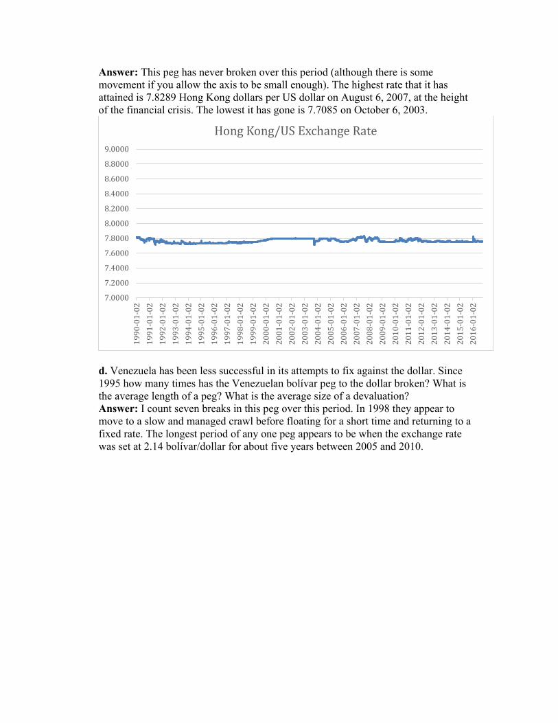
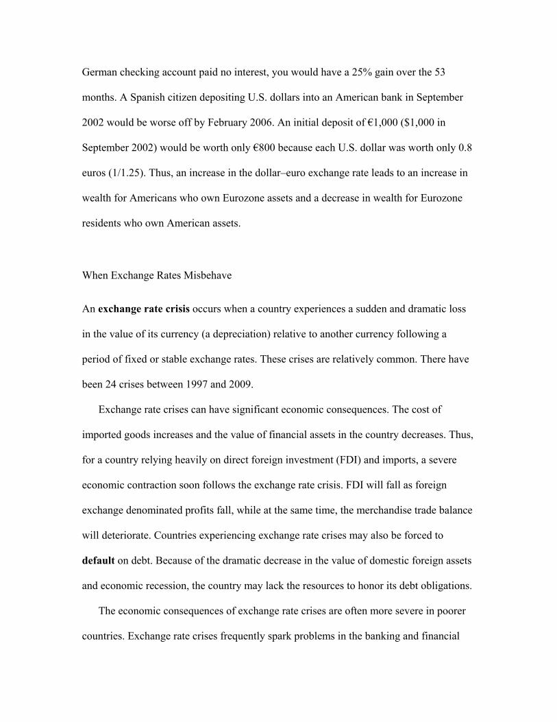
b. How would you characterize the relationship between the rupee and the dollar from 1998–2008? Does it appear to be fixed, crawling, or floating during this period? How would you characterize it from 2008 onward? Answer: Over this period the exchange rate appears to be a crawling peg. Although this crawl is relatively flat for a few years at the beginning of this period, it appears free to move. However, the lack of short-term volatility suggests that the exchange rate is still being controlled and is hence crawling. From 2008 onward this appears to be a freely floating currency. The line becomes more erratic with a greater deal of short-term volatility. c. The Hong Kong dollar has maintained its peg with the United States dollar since 1983. Over the course of the period that you have downloaded what are the highest and lowest values for this exchange rate?
0.0000
10.0000
20.0000
30.0000
40.0000
50.0000
60.0000
70.0000
80.0000
1990
-01-
0219
91-0
1-02
1992
-01-
0219
93-0
1-02
1994
-01-
0219
95-0
1-02
1996
-01-
0219
97-0
1-02
1998
-01-
0219
99-0
1-02
2000
-01-
0220
01-0
1-02
2002
-01-
0220
03-0
1-02
2004
-01-
0220
05-0
1-02
2006
-01-
0220
07-0
1-02
2008
-01-
0220
09-0
1-02
2010
-01-
0220
11-0
1-02
2012
-01-
0220
13-0
1-02
2014
-01-
0220
15-0
1-02
2016
-01-
02
Rupee/Dollar Exchange Rate
International Macroeconomics 4th Edition Feenstra Solutions ManualFull Download: https://testbanklive.com/download/international-macroeconomics-4th-edition-feenstra-solutions-manual/
Full download all chapters instantly please go to Solutions Manual, Test Bank site: testbanklive.com
Answer: This peg has never broken over this period (although there is some movement if you allow the axis to be small enough). The highest rate that it has attained is 7.8289 Hong Kong dollars per US dollar on August 6, 2007, at the height of the financial crisis. The lowest it has gone is 7.7085 on October 6, 2003.
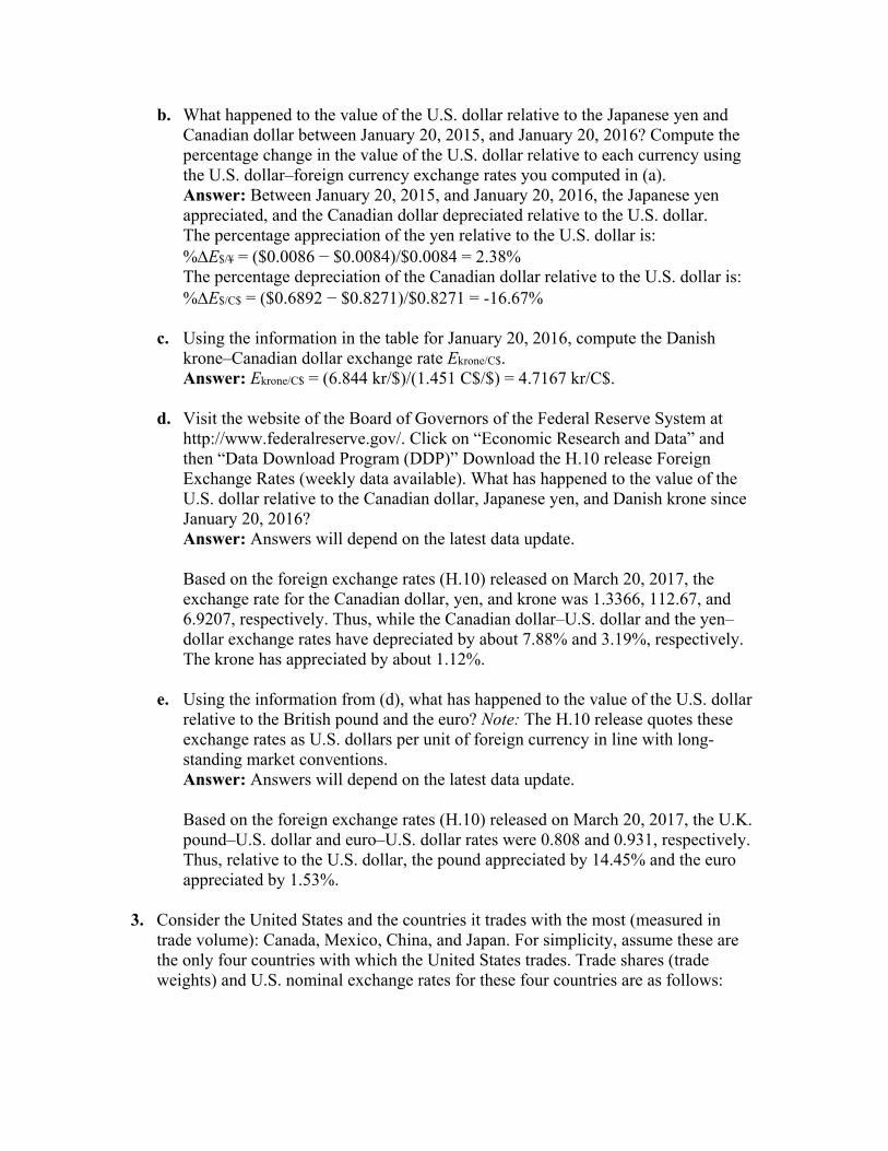
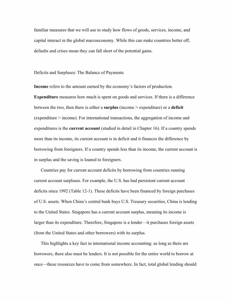
d. Venezuela has been less successful in its attempts to fix against the dollar. Since 1995 how many times has the Venezuelan bolívar peg to the dollar broken? What is the average length of a peg? What is the average size of a devaluation? Answer: I count seven breaks in this peg over this period. In 1998 they appear to move to a slow and managed crawl before floating for a short time and returning to a fixed rate. The longest period of any one peg appears to be when the exchange rate was set at 2.14 bolívar/dollar for about five years between 2005 and 2010.
7.0000
7.2000
7.4000
7.6000
7.8000
8.0000
8.2000
8.4000
8.6000
8.8000
9.000019
90-0
1-02
1991
-01-
0219
92-0
1-02
1993
-01-
0219
94-0
1-02
1995
-01-
0219
96-0
1-02
1997
-01-
0219
98-0
1-02
1999
-01-
0220
00-0
1-02
2001
-01-
0220
02-0
1-02
2003
-01-
0220
04-0
1-02
2005
-01-
0220
06-0
1-02
2007
-01-
0220
08-0
1-02
2009
-01-
0220
10-0
1-02
2011
-01-
0220
12-0
1-02
2013
-01-
0220
14-0
1-02
2015
-01-
0220
16-0
1-02
Hong Kong/US Exchange Rate
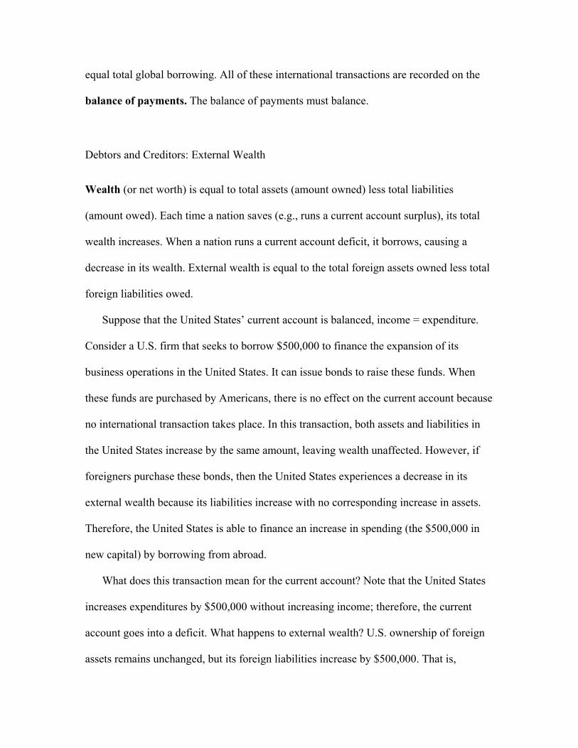
2. Refer to the exchange rates given in the following table:
January 20, 2016 January 20, 2015 Country (currency) FX per $ FX per £ FX per € FX per $ Australia (dollar) 1.459 2.067 1.414 1.223 Canada (dollar) 1.451 2.056 1.398 1.209 Denmark (krone) 6.844 9.694 7.434 6.430 Eurozone (euro) 0.917 1.299 1.000 0.865 Hong Kong (dollar) 7.827 11.086 8.962 7.752 India (rupee) 68.05 96.39 71.60 61.64 Japan (yen) 116.38 164.84 136.97 118.48 Mexico (peso) 18.60 26.346 16.933 14.647 Sweden (krona) 8.583 12.157 9.458 8.181 United Kingdom (pound) 0.706 1.000 0.763 0.600 United States (dollar) 1.000 1.416 1.156 1.000
Data from: U.S. Federal Reserve Board of Governors, H.10 release: Foreign Exchange Rates. Based on the table provided, answer the following questions: a. Compute the U.S. dollar–yen exchange rate E$/¥ and the U.S. dollar–Canadian
dollar exchange rate E$/C$ on January 20, 2016, and January 20, 2015. Answer: U.S. dollar–yen rates: January 20, 2015: E$/¥ = 1/(118.48) = $0.0084/¥ January 20, 2016: E$/¥ = 1/(116.38) = $0.0086/¥ January 20, 2015: E$/C$ = 1/(1.209) = $0.8271/C$ January 20, 2016: E$/C$ = 1/(1.451) = $0.6892/C$
0
2
4
6
8
10
12
Venezuela/US Exchange Rate
b. What happened to the value of the U.S. dollar relative to the Japanese yen and Canadian dollar between January 20, 2015, and January 20, 2016? Compute the percentage change in the value of the U.S. dollar relative to each currency using the U.S. dollar–foreign currency exchange rates you computed in (a).
Answer: Between January 20, 2015, and January 20, 2016, the Japanese yen appreciated, and the Canadian dollar depreciated relative to the U.S. dollar.
The percentage appreciation of the yen relative to the U.S. dollar is: %∆E$/¥ = ($0.0086 − $0.0084)/$0.0084 = 2.38% The percentage depreciation of the Canadian dollar relative to the U.S. dollar is: %∆E$/C$ = ($0.6892 − $0.8271)/$0.8271 = -16.67% c. Using the information in the table for January 20, 2016, compute the Danish
krone–Canadian dollar exchange rate Ekrone/C$. Answer: Ekrone/C$ = (6.844 kr/$)/(1.451 C$/$) = 4.7167 kr/C$. d. Visit the website of the Board of Governors of the Federal Reserve System at
http://www.federalreserve.gov/. Click on “Economic Research and Data” and then “Data Download Program (DDP)” Download the H.10 release Foreign Exchange Rates (weekly data available). What has happened to the value of the U.S. dollar relative to the Canadian dollar, Japanese yen, and Danish krone since January 20, 2016?
Answer: Answers will depend on the latest data update. Based on the foreign exchange rates (H.10) released on March 20, 2017, the
exchange rate for the Canadian dollar, yen, and krone was 1.3366, 112.67, and 6.9207, respectively. Thus, while the Canadian dollar–U.S. dollar and the yen–dollar exchange rates have depreciated by about 7.88% and 3.19%, respectively. The krone has appreciated by about 1.12%.
e. Using the information from (d), what has happened to the value of the U.S. dollar
relative to the British pound and the euro? Note: The H.10 release quotes these exchange rates as U.S. dollars per unit of foreign currency in line with long-standing market conventions.
Answer: Answers will depend on the latest data update. Based on the foreign exchange rates (H.10) released on March 20, 2017, the U.K.
pound–U.S. dollar and euro–U.S. dollar rates were 0.808 and 0.931, respectively. Thus, relative to the U.S. dollar, the pound appreciated by 14.45% and the euro appreciated by 1.53%.
3. Consider the United States and the countries it trades with the most (measured in
trade volume): Canada, Mexico, China, and Japan. For simplicity, assume these are the only four countries with which the United States trades. Trade shares (trade weights) and U.S. nominal exchange rates for these four countries are as follows:
Country (currency) Share of Trade $ per FX in 2015 $ per FX in 2016 Canada (dollar) 36% 0.8271 0.6892 Mexico (peso) 28% 0.0683 0.0538 China (yuan) 20% 0.1608 0.1522 Japan (yen) 16% 0.0080 0.0086
a. Compute the percentage change from 2015 to 2016 in the four U.S. bilateral
exchange rates (defined as U.S. dollars per unit of foreign exchange, or FX) in the table provided.
Answer: %∆E$/C$ = (0.6892 − 0.8271)/0.8271 = −16.67% %∆E$/pesos = (0.0538 − 0.0683)/0.0683 = −21.23% %∆E$/yuan = (0.1522 − 0.1608)/0.1608 = −5.35% %∆E$/¥ = (0.0086 − 0.008/0.008 = 7.50% b. Use the trade shares as weights to compute the percentage change in the nominal
effective exchange rate for the United States between 2015 and 2016 (in U.S. dollars per foreign currency basket).
Answer: The trade-weighted percentage change in the exchange rate is: %∆E = 0.36(%∆E$/C$) + 0.28(%∆E$/pesos) + 0.20(%∆E$/yuan) + 0.16(%∆E$/¥) %∆E = 0.36(−16.67 %) + 0.28(−21.23%) + 0.20(−5.35%) + 0.16(7.50%) = −11.82% c. Based on your answer to (b), what happened to the value of the U.S. dollar against
this basket between 2015 and 2016? How does this compare with the change in the value of the U.S. dollar relative to the Mexican peso? Explain your answer.
Answer: The dollar appreciated by 11.82% against the basket of currencies. Vis-à-vis the peso, the dollar appreciated by 21.23%. The average depreciation is smaller because the dollar depreciated by only 5.35% against China with a 20% trade share and appreciated against the yen with a 16% trade share.
4. Go to the FRED website: http://research.stlouisfed.org/fred2/. Locate the monthly
exchange rate data for the following: Look at the graphs and make your own judgment as to whether each currency was
fixed (peg or band), crawling (peg or band), or floating relative to the U.S. dollar during each time frame given.
a. Canada (dollar), 1980–2012 Answer: Floating exchange rate b. China (yuan), 1999–2004, 2005–09, and 2009–10 Answer: 1999–2004: fixed exchange rate; 2005–09: gradual appreciation vis-à-
vis the dollar; again fixed for 2009–10 c. Mexico (peso), 1993–95 and 1995–2012 Answer: 1993–95: crawl; 1995–2012: floating (with some evidence of a managed
float) d. Thailand (baht), 1986–97 and 1997–2012 Answer: 1986–97: fixed exchange rate; 1997–2012: floating e. Venezuela (bolívar), 2003–12 Answer: fixed exchange rate (with occasional adjustments) 5. Describe the different ways in which the government may intervene in the forex
market. Why does the government have the ability to intervene in this way, while private actors do not?
Answer: The government may participate in the forex market in a number of ways: capital controls, establishing an official market (with fixed rates) for forex transactions, and forex intervention by buying and selling currencies in the forex markets. The government has the ability to intervene in a way that private actors do not because through its central bank it has unlimited stock of its own currency and usually a large stock of foreign reserves. Its intervention is guided by policy rather than merely making profits on currency trade, which is the case with the private sector.
Work it out. Consider a Dutch investor with 1,000 euros to place in a bank deposit in
either the Netherlands or Great Britain. The (one-year) interest rate on bank deposits is 1% in Britain and 5% in the Netherlands. The (one-year) forward euro–pound exchange rate is 1.65 euros per pound and the spot rate is 1.5 euros per pound. Answer the following questions, using the exact equations for uncovered interest parity (UIP) and covered interest parity (CIP) as necessary.
a. What is the euro-denominated return on Dutch deposits for this investor? Answer: The investor’s return on euro-denominated Dutch deposits is equal to
€1,050 = €1,000 × (1 + 0.05). b. What is the (riskless) euro-denominated return on British deposits for this investor
using forward cover? Answer: The euro-denominated return on British deposits using forward cover is
equal to €1,111 (= €1,000 × (1.65/1.5) × (1 + 0.01)). c. Is there an arbitrage opportunity here? Explain why or why not. Is this an
equilibrium in the forward exchange rate market? Answer: Yes, there is an arbitrage opportunity. The euro-denominated return on
British deposits is higher than that on Dutch deposits. The net return on each euro deposit in a Dutch bank is equal to 5% versus 11.1% (= (1.65/1.5) × (1 + 0.01)) on a British deposit (using forward cover). This is not an equilibrium in the forward exchange market. The actions of traders seeking to exploit the arbitrage opportunity will cause the spot and forward rates to change.
d. If the spot rate is 1.5 euros per pound, and interest rates are as stated previously, what is the equilibrium forward rate, according to CIP?
Answer: CIP implies F€/£ = E€/£ (1 + i€)/(1 + i£) = 1.65 × 1.05/1.01 = €1.72 per £. e. Suppose the forward rate takes the value given by your answer to (d). Compute
the forward premium on the British pound for the Dutch investor (where exchange rates are in euros per pound). Is it positive or negative? Why do investors require this premium/discount in equilibrium?
Answer: Forward premium = (F€/£/E€/£ − 1) = (1.72/1.50) − 1 = 0.1467 or 14.67%. The existence of a positive forward premium would imply that investors expect the euro to depreciate relative to the British pound. Therefore, when establishing forward contracts, the forward rate is higher than the current spot rate.
f. If UIP holds, what is the expected depreciation of the euro (against the pound)
over one year? Answer: If UIP holds, the expected euro–pound exchange rate is the same as the
forward rate, that is, € 1.72 per £ (see part (d) above). The expected depreciation of Euro against pound is therefore 14.67%.
g. Based on your answer to (f), what is the expected euro–pound exchange rate one
year ahead? Answer: Following the answer to parts (d) and (f), the expected euro–pound
exchange rate is €1.72 per £ or 1/1.72 = 0.5814 £/€. 6. Suppose quotes for the dollar–euro exchange rate E$/€ are as follows: in New York
$1.05 per euro, and in Tokyo $1.15 per euro. Describe how investors use arbitrage to take advantage of the difference in exchange rates. Explain how this process will affect the dollar price of the euro in New York and Tokyo.
Answer: Investors will buy euros in New York at a price of $1.05 each because this is relatively cheaper than the price in Tokyo. They will then sell these euros in Tokyo at a price of $1.15, earning a $0.10 profit on each euro. With the influx of buyers in New York, the price of euros in New York will increase. With the influx of traders selling euros in Tokyo, the price of euros in Tokyo will decrease. This price adjustment continues until the exchange rates are equal in both markets.
7. You are a financial adviser to a U.S. corporation that expects to receive a payment of
60 million Japanese yen in 180 days for goods exported to Japan. The current spot rate is 100 yen per U.S. dollar (E$/¥ = 0.01000). You are concerned that the U.S. dollar is going to appreciate against the yen over the next six months.
a. Assuming the exchange rate remains unchanged, how much does your firm expect
to receive in U.S. dollars? Answer: The firm expects to receive $600,000 (= ¥60,000,000/100).
b. How much would your firm receive (in U.S. dollars) if the dollar appreciated to
110 yen per U.S. dollar (E$/¥ = 0.00909)? Answer: The firm would receive $545,454 (= ¥60,000,000/110). c. Describe how you could use an options contract to hedge against the risk of losses
associated with the potential appreciation in the U.S. dollar. Answer: The firm could buy ¥60 million in call options on dollars, say, for
example, at a rate of 105¥ per dollar. A call option gives the buyer a right to buy dollars at the price agreed upon. If the dollar appreciates such that its price rises above 105¥, say to 110¥, the firm will exercise the option. This ensures the firm’s yen receipts will at least be worth $571,428 (= ¥60,000,000/105).
8. Consider how transactions costs affect foreign currency exchange. Rank each of the
following foreign exchanges according to their probable spread (between the “buy at” and “sell for” bilateral exchange rates) and justify your ranking.
a. An American returning from a trip to Turkey wants to exchange his Turkish lira
for U.S. dollars at the airport. b. Citigroup and HSBC, both large commercial banks located in the United States
and United Kingdom, respectively, need to clear several large checks drawn on accounts held by each bank.
c. Honda Motor Company needs to exchange yen for U.S. dollars to pay American workers at its Ohio manufacturing plant.
d. A Canadian tourist in Germany pays for her hotel room using a credit card. Answer: Ranking (highest spread first): (a), (d), (c), (b). Both (a) and (d) involve
small transactions that will involve a go-between who will charge a premium to convert the currency. (d) involves a credit card company (a commercial bank or nonbank financial institution) that likely is involved in large volumes of transactions each day. (c) involves a corporation that can negotiate a better rate (versus an individual) because it will likely engage in a large currency exchange, or Honda could simply enter the market without going through a broker. Finally, (b) involves two large commercial banks that regularly engage in large-volume foreign exchange trading.
12 The Global Macroeconomy
Notes to the Instructor
Chapter Summary
This chapter provides students with a broad overview of international macroeconomics.
The chapter uses several key concepts to introduce the subject to students without formal
modeling. At the end of each topic, there are two sections that review the content of the
section (Key Topics) and prepare students for what’s coming next (Summary and Plan of
Study).
Comments
Instructors may want to cover this chapter in several lectures or in one short lecture. But
remember, this chapter is an overview. Don’t fall into the trap of trying to cover too much
detail. There are 10 more chapters to take care of that! However, covering this chapter in
detail at the beginning may serve to motivate students’ interest in the topic. If students
read through the chapter without a guided lecture, they may become overwhelmed.
Chapter 12 tackles complicated concepts to give students an idea of the topics that will be
covered through the rest of the textbook.
Plan of Study Each of the topics in this chapter concludes with a plan of study that discusses how
selected chapters in the text relate to the three broad elements presented in the
introduction: money, finance, and policy. An overview of these chapters is given below.
In the lecture notes, the plan of study for each of these topics is included in the summary.
1. Exchange rates (Chapters 13–15)
a. Overview of the foreign exchange market (Chapter 13)
b. Theory of exchange rate behavior in the long run: The monetary approach
(Chapter 14)
c. Theory of exchange rate behavior in the short run: The asset approach
(Chapter 15)
2. Balance of payments (Chapters 16–18)
a. Overview of balance of payments (BOP) and national income accounting
(Chapter 16)
b. The relationship between the BOP, the nation’s wealth, and living standards in
the long run (Chapter 17)
c. The relationship between the BOP, exchange rates, and the demand for output
in the short run (Chapter 18)
3. Exchange rate regimes and institutions (Chapters 19–22)
a. Overview of fixed and floating exchange rate regimes (Chapter 19)
b. Exchange rate crisis (Chapter20)
c. The Eurozone and the theory of optimum currency areas (Chapter 21)
d. Further topics in international macroeconomics (Chapter 22)
Key Topics
Each topic and subtopic in this chapter include discussion questions that tie these broad
topics together, as well as look forward to future chapters in the text.
Lecture Notes
Three key elements (corresponding to parts 1–3 of the chapter in organization):
■ Money: Many different currencies are used in the world today. Why? What is
their purpose? What are the implications of using so many different currencies?
■ Finance: Capital is more mobile internationally—the scale of international
finance is immense. Why? What is the purpose of this? Who lends/borrows? Who
benefits? What are the costs and to whom do they accrue?
■ Policy: The role of the government. How are economic policy failures
understood? What is the role of government in perpetuating/preventing these
events? What are the trade-offs?
1 Foreign Exchange: Currencies and Crises The exchange rate is the price of a foreign currency. Therefore, when countries trade
goods and services or engage in financial transactions with each other, the exchange rate
is one of the main factors that determine the prices that will be used. When an individual
buys a product, such as a car, the components of this product may come from all over the
world. At each step of the production process, the exchange rate affects the costs of
producing this good and, therefore, the price that one pays in domestic currency.
How Exchange Rates Behave Exchange rate regimes can be divided into two broad groups: floating and fixed. Floating
exchange rates are those that change frequently, implying that the price of one currency
changes relative to another. For example, the euro–dollar exchange rate has changed as
much as 5% within a single month. These changes are a reflection of changes in the
demand and supply of each currency in the foreign exchange market, which is studied in
the next chapter.
Fixed exchange rates are those that remain relatively constant over time, such that the
price of the currencies relative to one another is stable. For example, the yuan–dollar
exchange rate has remained relatively constant with only occasional adjustments. These
occasional adjustments are not accidental. They are the result of deliberate government
policy.
Why Exchange Rates Matter There are two channels through which the exchange rate affects the economy: relative
prices of goods and relative prices of assets. When the exchange rate changes, this affects
the price people pay for goods imported from abroad. Similarly, changes in the exchange
rate affect the price of financial assets abroad.
For example, a change in the dollar–euro exchange rate (the dollar price of a euro)
from $1 per euro in September 2002 to $1.25 per euro in February 2006 affected the
prices that Americans paid for European goods and the prices Europeans paid for
American goods. To see why, consider the price of a pair of leather boots that initially
cost $100 in the United States and €100 in Europe during September 2002. When the
exchange rate increases to $1.25 per euro, the relative price of these boots changes.
Americans buying Italian boots have to pay $125, whereas Europeans buying American
boots pay €80 ($100/$125 per euro). We can see that the increase in the dollar–euro
exchange rate implies an increase in the price of European goods purchased by
Americans and a decrease in the price of American goods purchased by Europeans.
Therefore, the relative price of European goods to American goods increases when the
dollar–euro exchange rate increases.
Not only consumers are affected by these changes in relative prices; producers are as
well. In the previous example, the producer of the Italian boots faces an increase in its
relative costs of manufacturing boots for export to the United States. If the Italian
manufacturer wants to avoid a decrease in sales to its U.S. market, it may choose to
continue charging $100 per pair of boots for export. However, if it hires workers and
materials in Europe, the Italian producer must continue to pay for these inputs in euros.
When it converts the $100 back into euros, the Italian producer only receives €80. Thus,
the Italian producer will face a decrease in its profits. The reverse is true for American
producers exporting to Europe. They can continue charging €100 per pair of boots (or
$125 converted into dollar terms), leading to an increase in profits.
Similarly, changes in exchange rates affect the relative prices of financial assets.
Suppose that you deposited $1,000 into a German checking account in September 2002.
The bank account balance would be denominated in euros. You used $1,000 to purchase
1,000 euros in September 2002, depositing that into your German checking account. If
you left the funds in this account until February 2006, you would still have €1,000, but
this €1,000 is now worth $1,250 because each euro is now worth $1.25. Even if the
German checking account paid no interest, you would have a 25% gain over the 53
months. A Spanish citizen depositing U.S. dollars into an American bank in September
2002 would be worse off by February 2006. An initial deposit of €1,000 ($1,000 in
September 2002) would be worth only €800 because each U.S. dollar was worth only 0.8
euros (1/1.25). Thus, an increase in the dollar‒euro exchange rate leads to an increase in
wealth for Americans who own Eurozone assets and a decrease in wealth for Eurozone
residents who own American assets.
When Exchange Rates Misbehave An exchange rate crisis occurs when a country experiences a sudden and dramatic loss
in the value of its currency (a depreciation) relative to another currency following a
period of fixed or stable exchange rates. These crises are relatively common. There have
been 24 crises between 1997 and 2009.
Exchange rate crises can have significant economic consequences. The cost of
imported goods increases and the value of financial assets in the country decreases. Thus,
for a country relying heavily on direct foreign investment (FDI) and imports, a severe
economic contraction soon follows the exchange rate crisis. FDI will fall as foreign
exchange denominated profits fall, while at the same time, the merchandise trade balance
will deteriorate. Countries experiencing exchange rate crises may also be forced to
default on debt. Because of the dramatic decrease in the value of domestic foreign assets
and economic recession, the country may lack the resources to honor its debt obligations.
The economic consequences of exchange rate crises are often more severe in poorer
countries. Exchange rate crises frequently spark problems in the banking and financial
sector, among households and firms, and in government finance. In extreme cases, they
can be associated with political and social instability, as in the example of Iceland in
2008 (see Headlines: Economic Crisis in Iceland).
Often these countries seek external help from foreign allies or from international
development organizations, such as the International Monetary Fund (IMF) or World
Bank. These agencies may loan the government money to mitigate the economic
consequences of an exchange rate crisis, but the costs of such loans can become
burdensome on society.
Summary and Plan of Study In subsequent chapters, we learn about the structure and operation of the foreign
exchange market (Chapter 13). Chapters 14 and 15 present the theory of exchange rates.
Chapter 16 discusses how exchange rates affect international transactions in assets. We
examine the short-run impact of exchange rates on the demand for goods in Chapter 18,
and with this understanding, Chapter 19 examines the trade-offs governments face as
they choose between fixed and floating exchange rates. Chapter 20 covers exchange rate
crises in detail and Chapter 21 the euro, a common currency used in many countries.
2 Globalization of Finance: Debts and Deficits Financial globalization has taken hold around the world. Competition among countries
has reduced barriers to financial flows. To understand the financial transactions among
countries, we need an accounting framework. Income, expenditure, and wealth are three
familiar measures that we will use to study how flows of goods, services, income, and
capital interact in the global macroeconomy. While this can make countries better off,
defaults and crises mean they can fall short of the potential gains.
Deficits and Surpluses: The Balance of Payments Income refers to the amount earned by the economy’s factors of production.
Expenditure measures how much is spent on goods and services. If there is a difference
between the two, then there is either a surplus (income > expenditure) or a deficit
(expenditure > income). For international transactions, the aggregation of income and
expenditures is the current account (studied in detail in Chapter 16). If a country spends
more than its income, its current account is in deficit and it finances the difference by
borrowing from foreigners. If a country spends less than its income, the current account is
in surplus and the saving is loaned to foreigners.
Countries pay for current account deficits by borrowing from countries running
current account surpluses. For example, the U.S. has had persistent current account
deficits since 1992 (Table 12-1). These deficits have been financed by foreign purchases
of U.S. assets. When China’s central bank buys U.S. Treasury securities, China is lending
to the United States. Singapore has a current account surplus, meaning its income is
larger than its expenditure. Therefore, Singapore is a lender—it purchases foreign assets
(from the United States and other borrowers) with its surplus.
This highlights a key fact in international income accounting: as long as there are
borrowers, there also must be lenders. It is not possible for the entire world to borrow at
once—these resources have to come from somewhere. In fact, total global lending should
equal total global borrowing. All of these international transactions are recorded on the
balance of payments. The balance of payments must balance.
Debtors and Creditors: External Wealth Wealth (or net worth) is equal to total assets (amount owned) less total liabilities
(amount owed). Each time a nation saves (e.g., runs a current account surplus), its total
wealth increases. When a nation runs a current account deficit, it borrows, causing a
decrease in its wealth. External wealth is equal to the total foreign assets owned less total
foreign liabilities owed.
Suppose that the United States’ current account is balanced, income = expenditure.
Consider a U.S. firm that seeks to borrow $500,000 to finance the expansion of its
business operations in the United States. It can issue bonds to raise these funds. When
these funds are purchased by Americans, there is no effect on the current account because
no international transaction takes place. In this transaction, both assets and liabilities in
the United States increase by the same amount, leaving wealth unaffected. However, if
foreigners purchase these bonds, then the United States experiences a decrease in its
external wealth because its liabilities increase with no corresponding increase in assets.
Therefore, the United States is able to finance an increase in spending (the $500,000 in
new capital) by borrowing from abroad.
What does this transaction mean for the current account? Note that the United States
increases expenditures by $500,000 without increasing income; therefore, the current
account goes into a deficit. What happens to external wealth? U.S. ownership of foreign
assets remains unchanged, but its foreign liabilities increase by $500,000. That is,
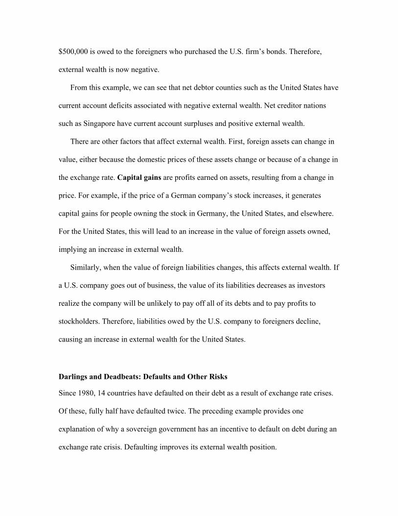
$500,000 is owed to the foreigners who purchased the U.S. firm’s bonds. Therefore,
external wealth is now negative.
From this example, we can see that net debtor counties such as the United States have
current account deficits associated with negative external wealth. Net creditor nations
such as Singapore have current account surpluses and positive external wealth.
There are other factors that affect external wealth. First, foreign assets can change in
value, either because the domestic prices of these assets change or because of a change in
the exchange rate. Capital gains are profits earned on assets, resulting from a change in
price. For example, if the price of a German company’s stock increases, it generates
capital gains for people owning the stock in Germany, the United States, and elsewhere.
For the United States, this will lead to an increase in the value of foreign assets owned,
implying an increase in external wealth.
Similarly, when the value of foreign liabilities changes, this affects external wealth. If
a U.S. company goes out of business, the value of its liabilities decreases as investors
realize the company will be unlikely to pay off all of its debts and to pay profits to
stockholders. Therefore, liabilities owed by the U.S. company to foreigners decline,
causing an increase in external wealth for the United States.
Darlings and Deadbeats: Defaults and Other Risks Since 1980, 14 countries have defaulted on their debt as a result of exchange rate crises.
Of these, fully half have defaulted twice. The preceding example provides one
explanation of why a sovereign government has an incentive to default on debt during an
exchange rate crisis. Defaulting improves its external wealth position.
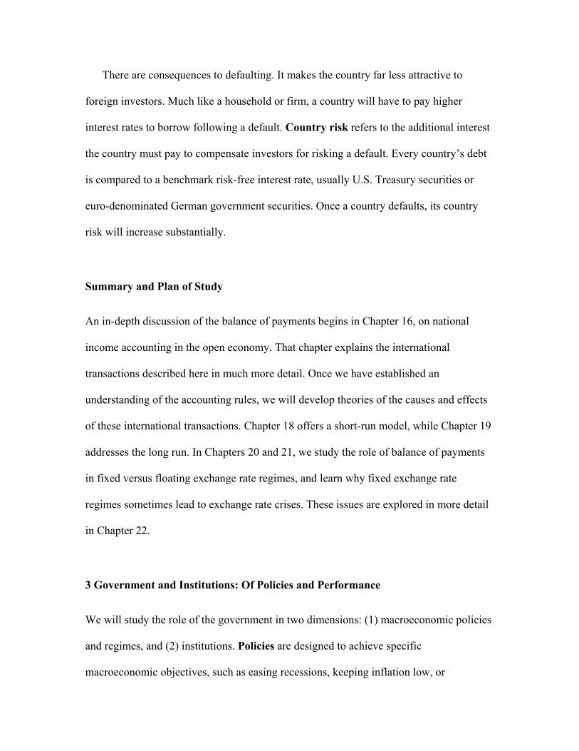
There are consequences to defaulting. It makes the country far less attractive to
foreign investors. Much like a household or firm, a country will have to pay higher
interest rates to borrow following a default. Country risk refers to the additional interest
the country must pay to compensate investors for risking a default. Every country’s debt
is compared to a benchmark risk-free interest rate, usually U.S. Treasury securities or
euro-denominated German government securities. Once a country defaults, its country
risk will increase substantially.
Summary and Plan of Study An in-depth discussion of the balance of payments begins in Chapter 16, on national
income accounting in the open economy. That chapter explains the international
transactions described here in much more detail. Once we have established an
understanding of the accounting rules, we will develop theories of the causes and effects
of these international transactions. Chapter 18 offers a short-run model, while Chapter 19
addresses the long run. In Chapters 20 and 21, we study the role of balance of payments
in fixed versus floating exchange rate regimes, and learn why fixed exchange rate
regimes sometimes lead to exchange rate crises. These issues are explored in more detail
in Chapter 22.
3 Government and Institutions: Of Policies and Performance We will study the role of the government in two dimensions: (1) macroeconomic policies
and regimes, and (2) institutions. Policies are designed to achieve specific
macroeconomic objectives, such as easing recessions, keeping inflation low, or
stabilizing interest rates. Policies are often made by the government. Examples of
macroeconomic policies include changes in the tax code or (in many countries) the
money supply. (In some countries, the money supply is not under the direct control of the
government. Examples include the U.S. and the European Monetary Union.) Regimes
refer to limitations on government discretion—the rules they must follow. Available
policy and regime choices depend on the institutions the economy supports.
As examples of policies, regimes, and institutions, consider three features of the
nation’s macroeconomic environment: integration and regulation of international finance,
independence and choice of exchange rate regime, and the role of institutions.
Integration and Capital Controls: The Regulation of International Finance Since 1970, there has been a general trend toward increased financial openness. There
has also been an increase in the volume of international financial transactions. But growth
in both areas has not been even across all countries. Consider three groups of countries
grouped according to their per capita income, economic growth, and degree of integration
into the global economy:
■ Advanced countries—high levels of per capita income and well integrated into
the global economy
■ Emerging markets—mainly middle-income countries that are growing and
becoming more integrated into the global economy
■ Developing countries—low-income countries that are not yet well integrated into
the global economy
The most dramatic increases in openness occurred in the early 1990s. During this
time, all three groups of countries adopted an increase in financial openness, with the
advanced economies benefiting from the largest increase in financial transactions. For
example, among advanced countries, the degree of financial openness approached 100%.
That same group saw foreign assets and liabilities rise to 5 times the GDP. Emerging and
developing countries lagged far behind in both these areas, with emerging markets only
achieving 50% financial openness and a doubling of the ratio of foreign assets and
liabilities to GDP.
Independence and Monetary Policy: The Choice of Exchange Rate Regimes There are two broad categories of exchange rate regimes: fixed and floating. Both are
common among the countries of the world. The choice of exchange rate regime is one of
the most important decisions a government can make. On the one hand, a fixed exchange
rate eliminates the uncertainty associated with exchange rate fluctuations (exchange rate
risk). In our previous examples, we saw that a change in the exchange rate affects relative
prices, profits, and external wealth. This uncertainty could potentially limit trade and
financial transactions. However, we have also seen that fixed exchange rates can lead to
exchange rate crises that are very costly.
The use of an individual currency is often viewed as part of the national identity,
something that establishes a country’s sovereignty. However, some groups of countries
have moved toward the adoption of a common currency. For example, as of 2009, the
Eurozone included 16 countries, each of which previously had its own currency. Other
countries have chosen to replace their own currency, using another country’s money as
their medium of exchange. Since the U.S. dollar is often used for this purpose, the policy
is called dollarization. El Salvador and Ecuador both dollarized their economies recently.
Institutions and Economic Performance: The Quality of Governance There are several different criteria for evaluating the quality of governance. This textbook
focuses on six: voice and accountability, political stability, government effectiveness,
regulatory quality, rule of law, and control of corruption. Better governance is strongly
associated with better economic outcomes. There is a positive relationship between good
governance and real income per person. And there is a somewhat weaker negative
correlation between good governance and the standard deviation of the rate of economic
growth. The differences are substantial, with advanced economies experiencing income
per person that is 50 times higher than the poorest developing countries. This gap in
living standards is known as The Great Divergence.
There is a negative relationship between quality institutions and income volatility.
Those countries with higher institutional quality tend to experience less volatility in
income. There are several reasons why this might be, including shifts in political power
and internal conflict.
We must confront the post hoc, ergo propter hoc fallacy here: Does the existence of
quality institutions lead to better economic outcomes? Or do good economic outcomes
make it possible to establish quality institutions? The research favors the first
explanation. Institutional quality appears to cause better economic outcomes. Given this
result, there is much debate about why poorer countries have weaker institutions.
Explanations include:
■ actions of colonizing powers (failure of colonization to establish quality
institutions)
■ differences in the evolution of legal codes that favored economic progress
■ differences in resource endowments that lead to the establishment of different
institutions according to geography
Summary and Plan of Study The government plays an important role in several facets of the international
macroeconomy. In Chapter 13, we will see how the government participates in the
foreign exchange market. In subsequent chapters, we will see how the government’s
choice of exchange rate regime is related to financial openness (Chapter 15), the benefits
of financial openness (Chapter 17), the trade-offs involved in the choice of regime
(Chapter 19), and how these decisions could lead to exchange rate crises (Chapter 20).
Chapter 21 studies the institutional design of the Eurozone. A key lesson from these
chapters is that governments must acknowledge the trade-offs involved in their choices
relating to discretionary policy, choice of regime, and the decision to adopt a common
currency.
4 Conclusions To understand the issues and debates surrounding exchange rates, the rise in international
financial transactions, and the role of institutions, we first need to understand how each
has changed over time. Then we move on to develop theories of how exchange rates and
international transactions affect the economy and the government’s role in this process.
Using these models helps us understand how the global macroeconomy works, what this
means for the growing gap between rich and poor countries, and how to evaluate policy
decisions.
TEACHING TIPS
Teaching Tip 1: One of the footnotes to Figure 12-5 cites M. Ayhan Kose, Eswar
Prasad, Kenneth S. Rogoff, and Shang-Jin Wei, 2006, “Financial Globalization: A
Reappraisal,” NBER Working Paper No. 12484. If your institution subscribes to the
NBER working paper series, you can download the paper from http://www.nber.org. If
not, the following page contains the list of countries included in each of the three major
categories: Advanced Economies, Emerging Market Economies, and Other Developing
Economies. Ask the class to study this list and discuss the countries that might have
moved to a different group since 2006. (Venezuela is one obvious example. That country
almost certainly can no longer be included in the emerging market group.)
Advanced Economies The 21 advanced industrial economies in our sample are Australia (AUS), Austria
(AUT), Belgium (BEL), Canada (CAN), Denmark (DNK), Finland (FIN), France (FRA),
Exchange Rate Quotations This table shows major exchange rates as they might appear in the financial media. Columns (1) to (3) show rates on December 31, 2015. For comparison, columns (4) to (6) show rates on December 31, 2014. For example, column (1) shows that at the end of 2015, one U.S. dollar was worth 1.501 Canadian dollars, 6.870 Danish krone, 0.921 euros, and so on. The euro–dollar rates appear in bold type.
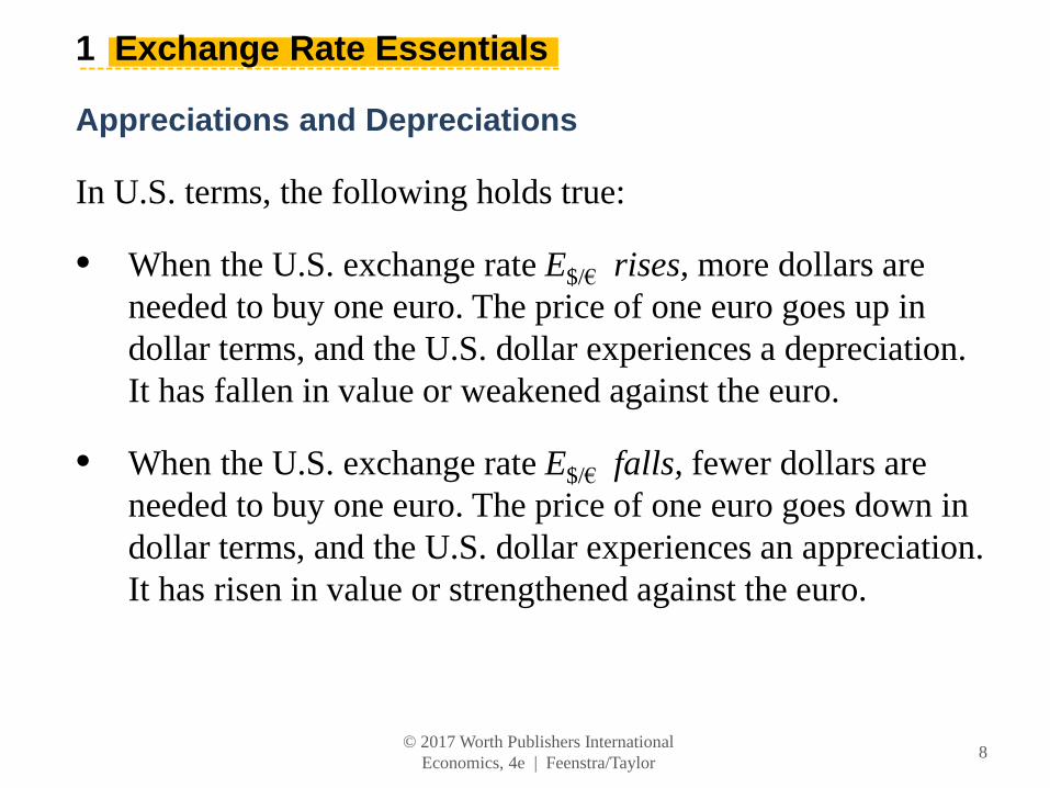
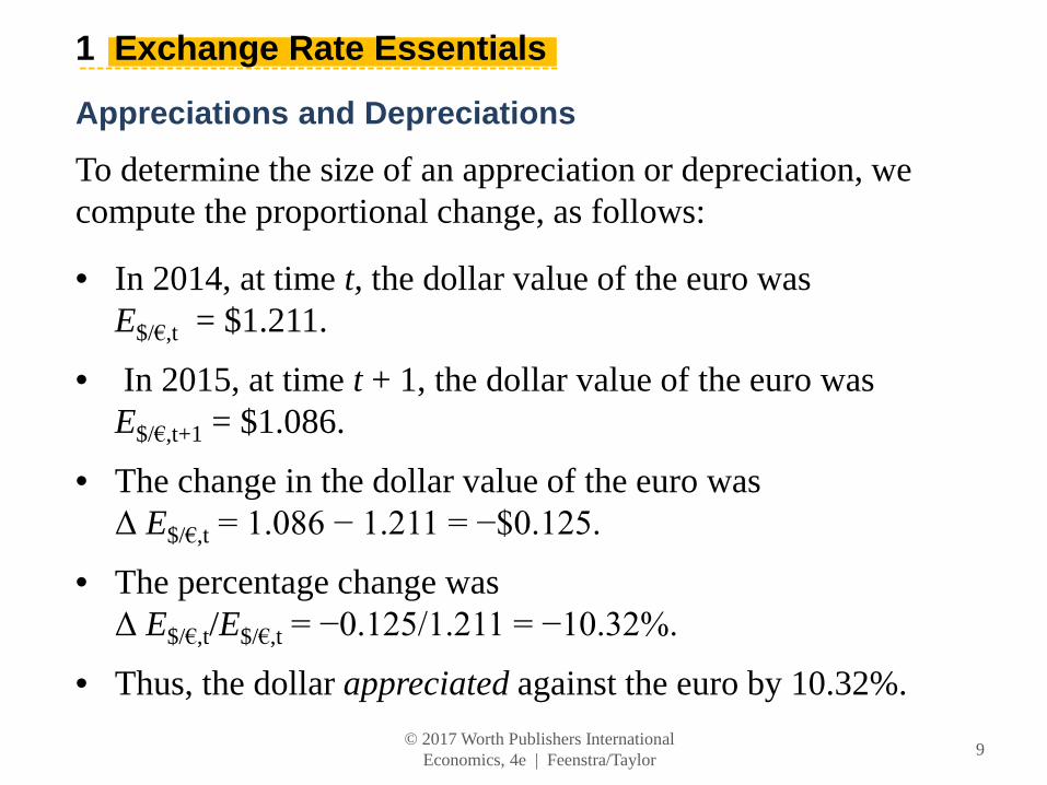
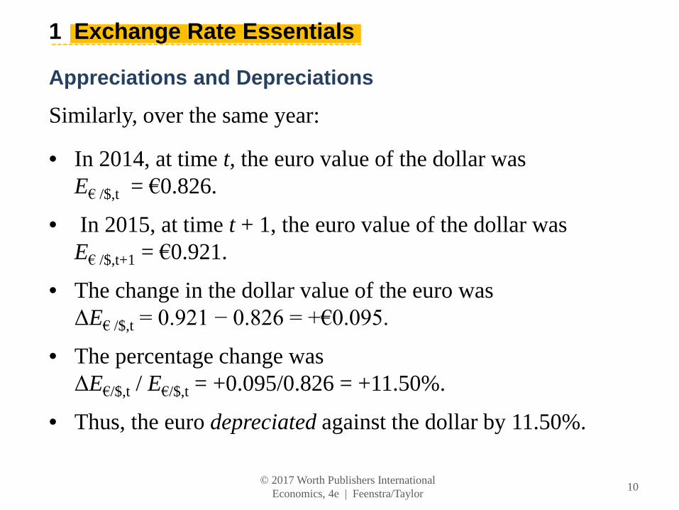
E$/€ = 1.086 = U.S. exchange rate (American terms)
• When the U.S. exchange rate E$/€ rises, more dollars are needed to buy one euro. The price of one euro goes up in dollar terms, and the U.S. dollar experiences a depreciation. It has fallen in value or weakened against the euro.
• When the U.S. exchange rate E$/€ falls, fewer dollars are needed to buy one euro. The price of one euro goes down in dollar terms, and the U.S. dollar experiences an appreciation. It has risen in value or strengthened against the euro.
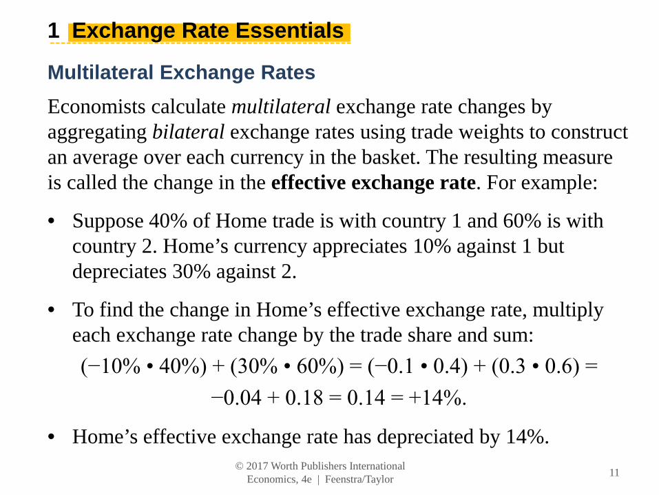
Economists calculate multilateral exchange rate changes by aggregating bilateral exchange rates using trade weights to construct an average over each currency in the basket. The resulting measure is called the change in the effective exchange rate. For example:
• Suppose 40% of Home trade is with country 1 and 60% is with country 2. Home’s currency appreciates 10% against 1 but depreciates 30% against 2.
• To find the change in Home’s effective exchange rate, multiply each exchange rate change by the trade share and sum:
In general, suppose there are N currencies in the basket, and Home’s trade with all N partners is:
Trade = Trade1 + Trade2 + . . . + TradeN.
Applying trade weights to each bilateral exchange rate change, the home country’s effective exchange rate (Eeffective) will change according to the following weighted average:
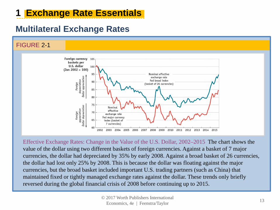
Effective Exchange Rates: Change in the Value of the U.S. Dollar, 2002–2015 The chart shows the value of the dollar using two different baskets of foreign currencies. Against a basket of 7 major currencies, the dollar had depreciated by 35% by early 2008. Against a broad basket of 26 currencies, the dollar had lost only 25% by 2008. This is because the dollar was floating against the major currencies, but the broad basket included important U.S. trading partners (such as China) that maintained fixed or tightly managed exchange rates against the dollar. These trends only briefly reversed during the global financial crisis of 2008 before continuing up to 2015.
Example: Using Exchange Rates to Compare Prices in a Common Currency
TABLE 2-2
Using the Exchange Rate to Compare Prices in a Common Currency Now pay attention, 007! This table shows how the hypothetical cost of James Bond’s next tuxedo in different locations depends on the exchange rates that prevail.
There are two major types of exchange rate regimes—
fixed and floating:
• A fixed (or pegged) exchange rate fluctuates in a narrow range (or not at all) against some base currency over a sustained period. The exchange rate can remain fixed for long periods only if the government intervenes in the foreign exchange market in one or both countries.
• A floating (or flexible) exchange rate fluctuates in a wider range, and the government makes no attempt to fix it against any base currency. Appreciations and depreciations may occur yearly, monthly, by the day, or even every minute.
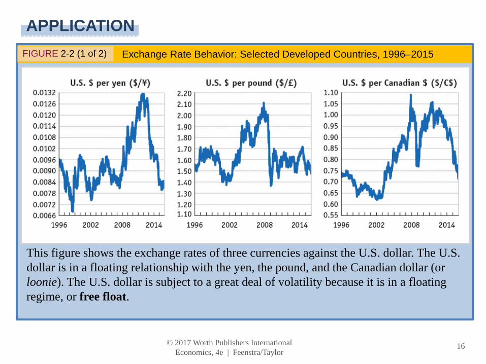
FIGURE 2-2 (1 of 2) Exchange Rate Behavior: Selected Developed Countries, 1996–2015
This figure shows the exchange rates of three currencies against the U.S. dollar. The U.S. dollar is in a floating relationship with the yen, the pound, and the Canadian dollar (or loonie). The U.S. dollar is subject to a great deal of volatility because it is in a floating regime, or free float.
FIGURE 2-2 (2 of 2) Exchange Rate Behavior: Selected Developed Countries, 1996–2015 (cont.)
This figure shows exchange rates of three currencies against the euro, which was introduced in 1999. The pound and the yen float against the euro. The Danish krone provides an example of a fixed exchange rate. There is only a tiny variation around this rate, no more than plus or minus 2%. This type of fixed regime is known as a band.
Selected Developing Countries, 1996–2015 Exchange rates in developing countries show a wide variety of experiences and greater volatility. Pegging is common but is punctuated by periodic crises (you can see the effects of these crises in graphs for Thailand, South Korea, and India).
India is an example of a middle ground, somewhere between a fixed rate and a free float, called a managed float. Colombia is an example of a crawling peg. The Colombian peso is allowed to crawl gradually, and it steadily depreciated at an almost constant rate for several years from 1996 to 2002. Dollarization occurred in Ecuador in 2000, a process that occurs when a country unilaterally adopts the currency of another country.
• Figure 2-4 shows an IMF classification of exchange rate regimes around the world, which allows us to see the prevalence of different regime types across the whole spectrum, from fixed to floating.
• The classification covers 182 economies for the year 2010, and regimes are ordered from the most rigidly fixed to the most freely floating.
• Six of these countries have a currency board, a type of fixed regime that has special legal and procedural rules designed to make the peg “harder”—that is, more durable.
This figure shows IMF classification of exchange rate regimes around the world for 182 economies in 2010. Regimes are ordered from the most rigidly fixed to the most freely floating. Six countries use an ultra-hard peg called a currency board, while 35 others have a hard peg.
FIGURE 2-4) A Spectrum of Exchange Rate Regimes (continued)
An additional 43 counties have bands, crawling pegs, or crawling bands, while 46 countries have exchange rates that either float freely, are managed floats, or are allowed to float within wide bands.
• The simplest forex transaction is a contract for the immediate exchange of one currency for another between two parties. This is known as a spot contract.
• The exchange rate for this transaction is often called the spot exchange rate.
• The use of the term “exchange rate” always refers to the spot rate for our purposes.
• The spot contract is the most common type of trade and appears in almost 90% of all forex transactions.
A forward contract differs from a spot contract in that the two parties make the contract today, but the settlement date for the delivery of the currencies is in the future, or forward. The time to delivery, or maturity, varies. However, because the price is fixed as of today, the contract carries no risk.
Swaps
A swap contract combines a spot sale of foreign currency with a forward repurchase of the same currency. This is a common contract for counterparties dealing in the same currency pair over and over again. Combining two transactions reduces transactions costs.
A futures contract is a promise that the two parties holding the contract will deliver currencies to each other at some future date at a prespecified exchange rate, just like a forward contract. Unlike the forward contract, futures contracts are standardized, mature at certain regular dates, and can be traded on an organized futures exchange.
Options
An option provides one party, the buyer, with the right to buy (call) or sell (put) a currency in exchange for another at a prespecified exchange rate at a future date. The buyer is under no obligation to trade and will not exercise the option if the spot price on the expiration date turns out to be more favorable.
Derivatives allow investors to engage in hedging (risk avoidance) and speculation (risk taking).
• Example 1: Hedging. As chief financial officer of a U.S. firm, you expect to receive payment of €1 million in 90 days for exports to France. The current spot rate is $1.20 per euro. Your firm will incur losses on the deal if the euro weakens to less than $1.10 per euro. You advise that the firm buy €1 million in call options on dollars at a rate of $1.15 per euro, ensuring that the firm’s euro receipts will sell for at least this rate. This locks in a minimal profit even if the spot rate falls below $1.15. This is hedging.
Derivatives allow investors to engage in hedging (risk avoidance) and speculation (risk taking).
• Example 2: Speculation. The market currently prices one-year euro futures at $1.30, but you think the dollar will weaken to $1.43 in the next 12 months. If you wish to make a bet, you would buy these futures, and if you are proved right, you will realize a 10% profit. Any level above $1.30 will generate a profit. If the dollar is at or below $1.30 a year from now, however, your investment in futures will be a total loss. This is speculation.
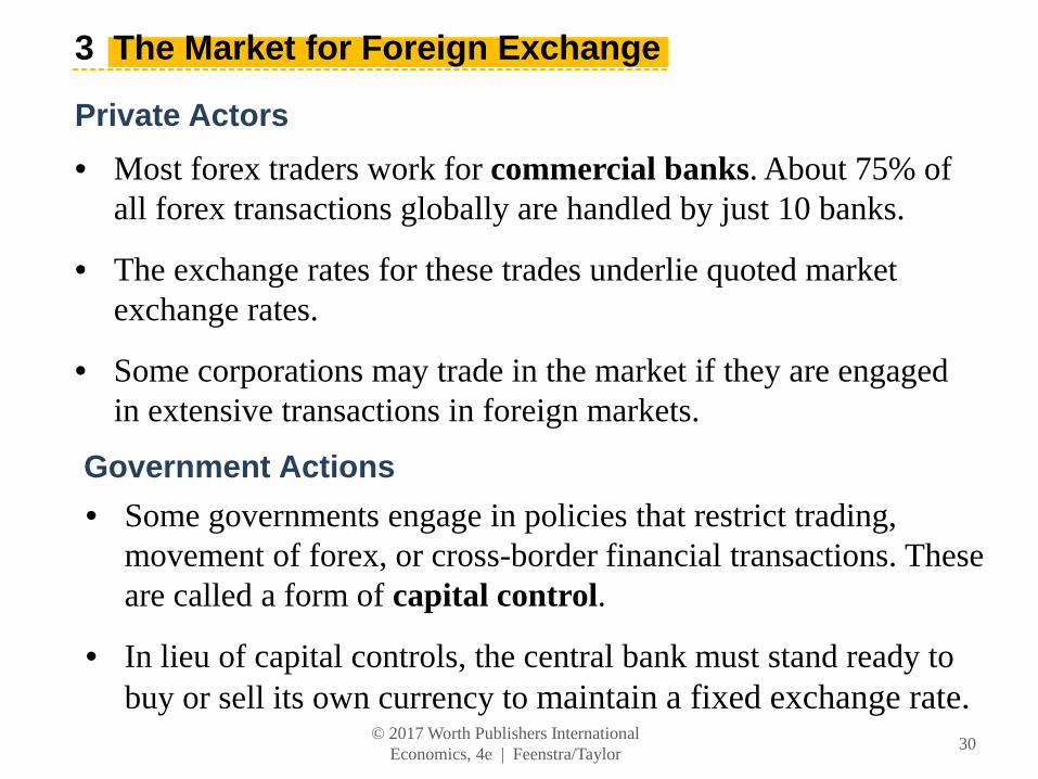
• Most forex traders work for commercial banks. About 75% of all forex transactions globally are handled by just 10 banks.
• The exchange rates for these trades underlie quoted market exchange rates.
• Some corporations may trade in the market if they are engaged in extensive transactions in foreign markets.
Government Actions
• Some governments engage in policies that restrict trading, movement of forex, or cross-border financial transactions. These are called a form of capital control.
• In lieu of capital controls, the central bank must stand ready to buy or sell its own currency to maintain a fixed exchange rate.
Arbitrage and Spot Rates Arbitrage ensures that the trade of currencies in New York along the path AB occurs at the same exchange rate as via London along path ACDB. At B the pounds received must be the same, regardless of the route taken to get to B:
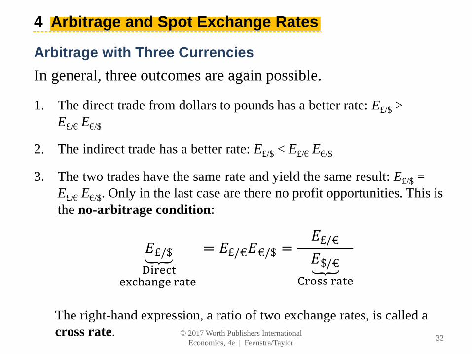
1. The direct trade from dollars to pounds has a better rate: E£/$ > E£/€ E€/$
2. The indirect trade has a better rate: E£/$ < E£/€ E€/$
3. The two trades have the same rate and yield the same result: E£/$ = E£/€ E€/$. Only in the last case are there no profit opportunities. This is the no-arbitrage condition:
Arbitrage and Cross Rates Triangular arbitrage ensures that the direct trade of currencies along the path AB occurs at the same exchange rate as via a third currency along path ACB. The pounds received at B must be the same on both paths:
• The majority of the world’s currencies trade directly with only one or two of the major currencies, such as the dollar, euro, yen, or pound.
• Many countries do a lot of business in major currencies such as the U.S. dollar, so individuals always have the option to engage in a triangular trade at the cross rate.
• When a third currency, such as the U.S. dollar, is used in these transactions, it is called a vehicle currency because it is not the home currency of either of the parties involved in the trade and is just used for intermediation.
An important question for investors is in which currency they should hold their liquid cash balances.
• Would selling euro deposits and buying dollar deposits make a profit for a banker?
• These decisions drive demand for dollars versus euros and the exchange rate between the two currencies.
The Problem of Risk
A trader in New York cares about returns in U.S. dollars. A dollar deposit pays a known return, in dollars. But a euro deposit pays a return in euros, and one year from now we cannot know for sure what the dollar–euro exchange rate will be.
• Riskless arbitrage and risky arbitrage lead to two important implications, called parity conditions.
Contracts to exchange euros for dollars in one year’s time carry an exchange rate of F$/€ dollars per euro. This is known as the forward exchange rate.
• If you invest in a dollar deposit, your $1 placed in a U.S. bank account will be worth (1 + i$) dollars in one year’s time. The dollar value of principal and interest for the U.S. dollar bank deposit is called the dollar return.
• If you invest in a euro deposit, you first need to convert the dollar to euros. Using the spot exchange rate, $1 buys 1/E$/€
euros today.
• These 1/E$/€ euros would be placed in a euro account earning i€, so in a year’s time they would be worth (1 + i€)/E$/€ euros.
To avoid that risk, you engage in a forward contract today to make the future transaction at a forward rate F$/€.
• The (1 + i€)/E$/€ euros you will have in one year’s time can then be exchanged for (1 + i€)F$/€/E$/€ dollars, or the dollar return on the euro bank deposit.
$/€
$/€
• This is called covered interest parity (CIP) because all exchange rate risk on the euro side has been “covered” by use of the forward contract.
Arbitrage and Covered Interest Parity Under CIP, returns to holding dollar deposits accruing interest going along the path AB must equal the returns from investing in euros going along the path ACDB with risk removed by use of a forward contract. Hence, at B, the riskless payoff must be the same on both paths:
FIGURE 2-9 (1 of 2) Financial Liberalization and Covered Interest Parity
Financial Liberalization and Covered Interest Parity: Arbitrage Between the United Kingdom and Germany The chart shows the difference in monthly pound returns on deposits in British pounds and German marks using forward cover from 1970 to 1995. In the 1970s, the difference was positive and often large: Traders would have profited from arbitrage by moving money from pound deposits to mark deposits, but capital controls prevented them from freely doing so.
FIGURE 2-9 (2 of 2) Financial Liberalization and Covered Interest Parity (continued)
After financial liberalization, these profits essentially vanished, and no arbitrage opportunities remained. The CIP condition held, aside from small deviations resulting from transactions costs and measurement errors.
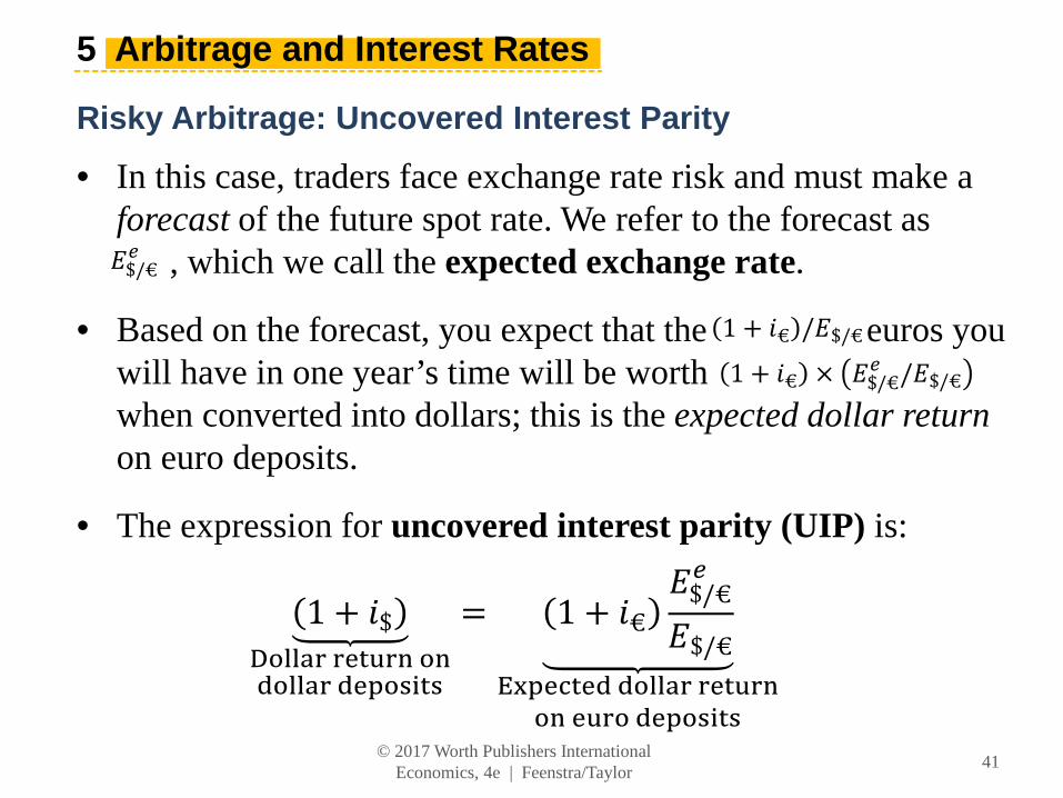
• In this case, traders face exchange rate risk and must make a forecast of the future spot rate. We refer to the forecast as
, which we call the expected exchange rate.
• Based on the forecast, you expect that the euros you will have in one year’s time will be worth when converted into dollars; this is the expected dollar returnon euro deposits.
• The expression for uncovered interest parity (UIP) is:
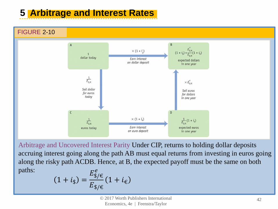
Arbitrage and Uncovered Interest Parity Under CIP, returns to holding dollar deposits accruing interest going along the path AB must equal returns from investing in euros going along the risky path ACDB. Hence, at B, the expected payoff must be the same on both paths:
• Uncovered interest parity is a no-arbitrage condition that describes an equilibrium in which investors are indifferent between the returns on unhedged interest-bearing bank deposits in two currencies.
• We can rearrange the terms in the uncovered interest parity expression to solve for the spot rate:
• An investor’s entire portfolio of assets may include stocks, bonds, real estate, art, bank deposits in various currencies, and so on. All assets have three key attributes that influence demand: return, risk, and liquidity.
• An asset’s rate of return is the total net increase in wealth resulting from holding the asset for a specified period of time, typically one year.
• The risk of an asset refers to the volatility of its rate of return.
• The liquidity of an asset refers to the ease and speed with which it can be liquidated, or sold.
• We refer to the forecast of the rate of return as the expected rate of return.
• Although the expected future spot rate and the forward rate are used in two different forms of arbitrage—risky and riskless, in equilibrium they should be exactly the same!
• If both covered interest parity and uncovered interest parity hold, the forward must equal the expected future spot rate.
• Risk-neutral investors have no reason to prefer to avoid risk by using the forward rate versus embracing risk by awaiting the future spot rate.
• If the forward rate equals the expected spot rate, the expected rate of depreciation equals the forward premium (the proportional difference between the forward and spot rates):
• While the left-hand side is easily observed, the expectations on the right-hand side are typically unobserved.
When UIP and CIP hold, the 12-month forward premium should equal the 12-month expected rate of depreciation. A scatterplot showing these two variables should be close to the diagonal 45-degree line.
Using evidence from surveys of individual forex traders’ expectations over the period 1988 to 1993, UIP finds some support, as the line of best fit is close to the diagonal.
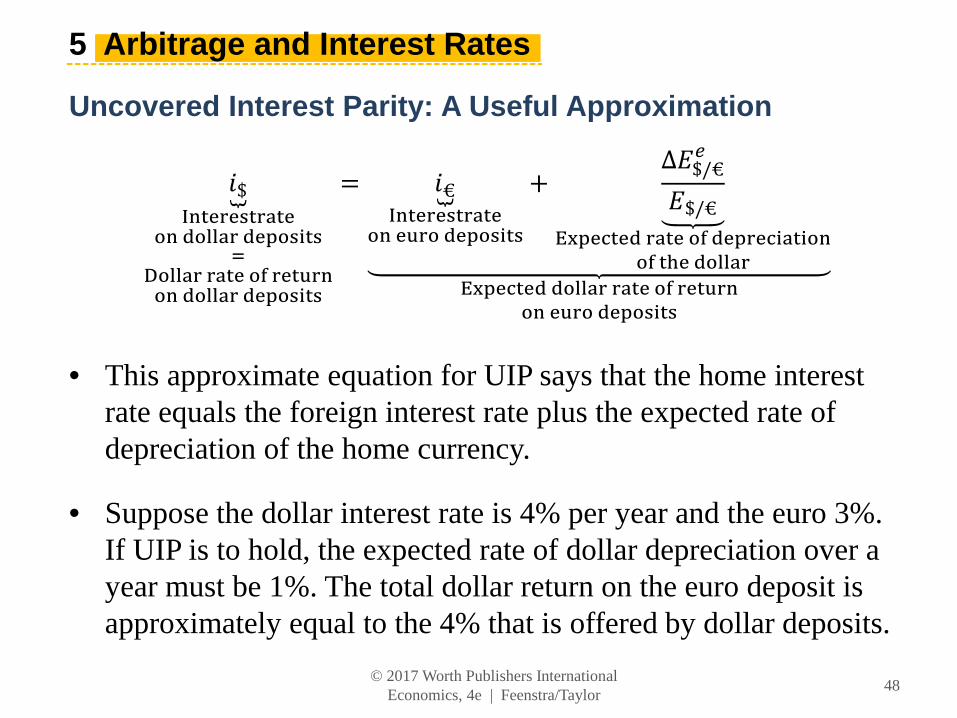
• This approximate equation for UIP says that the home interest rate equals the foreign interest rate plus the expected rate of depreciation of the home currency.
• Suppose the dollar interest rate is 4% per year and the euro 3%. If UIP is to hold, the expected rate of dollar depreciation over a year must be 1%. The total dollar return on the euro deposit is approximately equal to the 4% that is offered by dollar deposits.
How Interest Parity Relationships Explain Spot and Forward Rates In the spot market, UIP provides a model of how the spot exchange rate is determined. To use UIP to find the spot rate, we need to know the expected future spot rate and the prevailing interest rates for the two currencies. In the forward market, CIP provides a model of how the forward exchange rate is determined. When we use CIP, we derive the forward rate from the current spot rate (from UIP) and the interest rates for the two currencies.
1. The exchange rate in a country is the price of a unit of foreign currency expressed in terms of the home currency. This price is determined in the spot market for foreign exchange.
2. When the home exchange rate rises, less foreign currency is bought/sold per unit of home currency; the home currency has depreciated. If home currency buys x% less foreign currency, the home currency is said to have depreciated by x%.
3. When the home exchange rate falls, more foreign currency is bought/sold per unit of home currency; the home currency has appreciated. If home currency buys x% more foreign currency, the home currency is said to have appreciated by x%.
5. Exchange rates may be stable over time or they may fluctuate. History supplies examples of the former (fixed exchange rate regimes) and the latter (floating exchange rate regimes) as well as a number of intermediate regime types.
6. An exchange rate crisis occurs when the exchange rate experiences a sudden and large depreciation. These events are often associated with broader economic and political turmoil, especially in developing countries.
7. Some countries may forgo a national currency to form a currency union with other nations (e.g., the Eurozone), or they may unilaterally adopt the currency of another country (“dollarization”).
11. Arbitrage on currencies means that spot exchange rates are approximately equal in different forex markets. Cross rates (for indirect trades) and spot rates (for direct trades) are also approximately equal.
12. Riskless interest arbitrage leads to the covered interest parity (CIP) condition. CIP says that the dollar return on dollar deposits must equal the dollar return on euro deposits, where forward contracts are used to cover exchange rate risk.
14. Risky interest arbitrage leads to the uncovered interest parity (UIP) condition. UIP says that when spot contracts are used and exchange rate risk is not covered, the dollar return on dollar deposits must equal the expected dollar returns on euro deposits.
15. Uncovered interest parity explains how the spot rate is determined by the home and foreign interest rates and the expected future spot exchange rate.