RURAL DEVELOPMENT CHALLENGES: SYSTEM DYNAMICS EX ANTE DECISION SUPPORT FOR AGRICULTURAL INITIATIVES IN SOUTHERN MEXICO A Thesis Presented to the Faculty of the Graduate School of Cornell University In Partial Fulfillment of the Requirements for the Degree of Master of Professional Studies International Agriculture and Rural Development by Keenan Clay McRoberts January 2010
Transcript
RURAL DEVELOPMENT CHALLENGES:
SYSTEM DYNAMICS EX ANTE DECISION SUPPORT FOR
AGRICULTURAL INITIATIVES IN SOUTHERN MEXICO
A Thesis
Presented to the Faculty of the Graduate School
of Cornell University
In Partial Fulfillment of the Requirements for the Degree of
A persistent problem facing rural communities in the Gulf region of
Mexico is the low profitability of agriculture. In order to improve the short and
long-term economic security of households in these rural communities, value
addition to agricultural products is proposed by farmers and by professionals
for niche markets. Correspondingly, collective action in the form of rural
marketing cooperatives may provide a means to augment household profits
from sales of value-added products.
The ex ante assessment of this challenge, like others that are similarly
complex, is undertaken using system dynamics methods. In response to an
institutional request, researchers and development practitioners at the Instituto
Nacional de Investigaciones Forestales, Agrícolas y Pecuarias (INIFAP)
Xalapa team were trained in introductory systems thinking and dynamic
modeling techniques during a three-month, institutional capacity-building
course. When combined with INIFAP’s repertoire of technology and data
assessment tools, short course results suggested that system dynamics could
help fortify institutional capacity, especially ex ante problem assessment
capabilities.
A form of participatory model building in which small teams of course
participants complete the modeling process for selected dynamic problems
was incorporated into the short course. The teams achieved varying success
in the study and development of conceptual models and in building incipient
simulation models. The relative success of these learning-by-modeling
problem assessments reflected favorably on the high initial capacity and
motivation of the INIFAP-Xalapa team. This interdisciplinary team could
become an innovator in leading group model building initiatives to develop
more insightful alternative approaches for confronting complex agricultural
research and development problems and issues.
Course participants also completed group model building exercises and
contributed expert knowledge to improve a system dynamics model designed
to assess impacts on farmer profits of value-added agricultural production by a
smallholder marketing cooperative. The dynamic biophysical and
socioeconomic model consists of nine components that represent the
aggregate community flock and a value addition and marketing cooperative.
The primary objective of the model was to assess strategies to increase the
profitability of caprine production in highland communities. This adaptable
model was designed as an ex ante impact assessment mechanism for INIFAP
to evaluate policies and the associated opportunities and limitations of value
addition.
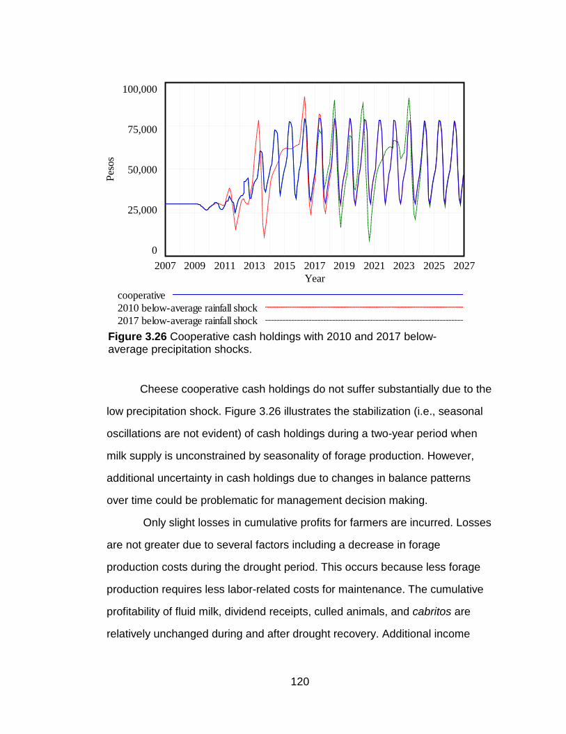
The analysis indicates that manufacture of value-added products from
goat’s milk by a rural dairy cooperative could increase community net income
from caprine activities under a wide variety of environmental and market
conditions. Increases in net income would be especially important during the
dry season, when cooperative dividend payments could partially mitigate
seasonality from typical other income sources. Model sensitivity analyses
demonstrated that the exogenous effects of seasonal rainfall on forage supply
are more important to system performance than endogenous feedback within
the system. System performance was measured primarily by elements that
likely influence farmer and cooperative decision-making: profitability of the
community goat flock, cooperative solvency time, dividend payments, and
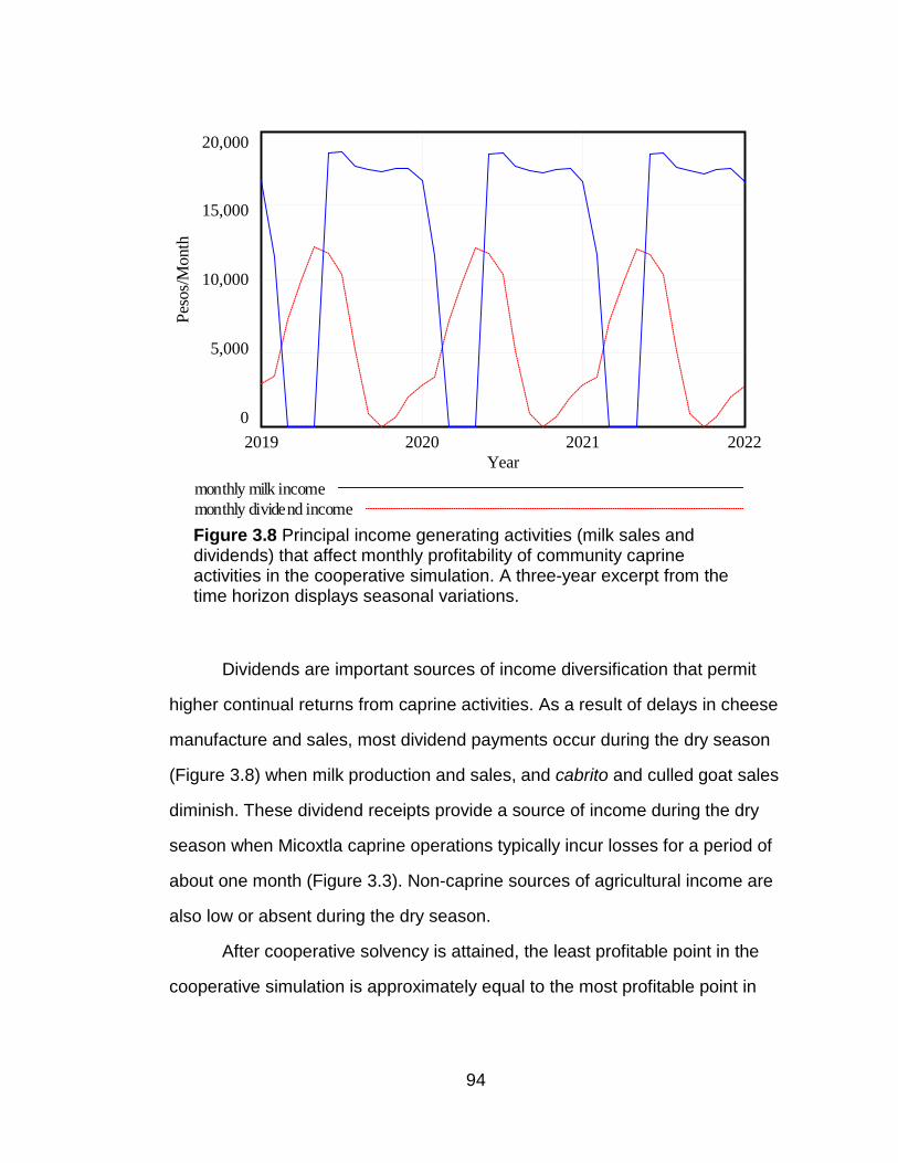
cancelled orders for aged cheese.
The analysis also indicated potential risks and those factors that could
limit cooperative success. The most important of such factors include the size
and reliability of the market for premium aged cheese, the cooperative’s
payments for milk and dividends, milk production costs, cheese production
costs, and the composition and productivity of the goat flock. These factors,
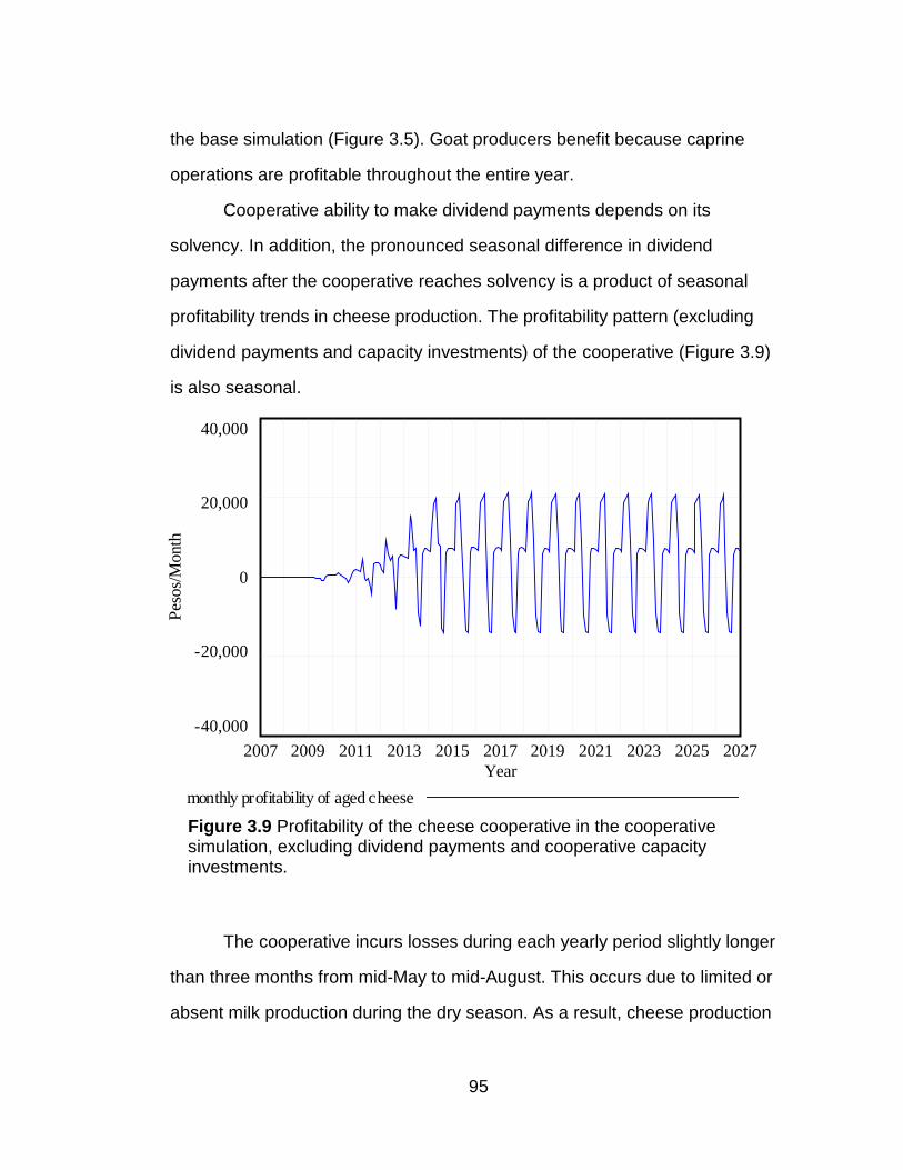
and forage quality, should receive priority in future research and
implementation.
iii
BIOGRAPHICAL SKETCH
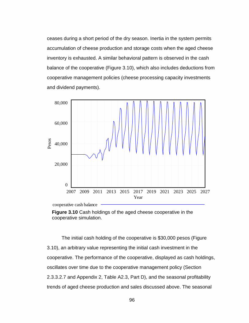
Keenan McRoberts grew up on a farm and exotic animal ranch in
western Nebraska. He received his B.S. in biochemistry from the University of
Nebraska-Lincoln. He then worked from 2001 to 2005 in northern Nicaragua
as an Agriculture Extension Volunteer and Agriculture Technical Trainer with
the Peace Corps. He entered the MPS program in International Agriculture
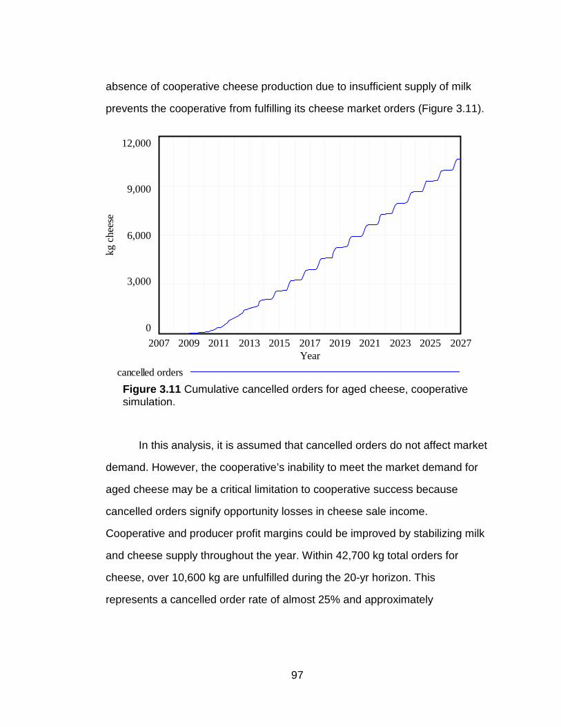
and Rural Development at Cornell University in 2006. He started a doctoral
program in Animal Science at Cornell University in summer 2009.
iv
To the INIFAP Team in Xalapa, Veracruz.
v
ACKNOWLEDGMENTS
Mil gracias al equipo de INIFAP en Xalapa por haberme recibido en
verano de 2007. Su dedicación al desarrollo de Veracruz es impresionante.
Les agradezco por haber abierto las puertas de su equipo para trabajar en
colaboración de beneficio mutuo conmigo. Ojalá que el curso y los modelos
que ustedes desarrollaron les haya servido. Su dedicación fue registrada por
su participación entusiasta y por su voluntad de aprender y aplicar los
métodos de dinámica de sistemas juntos con otras herramientas que ya se
utilizaron. Les deseo muy buena suerte con la dinámica de sistemas.
Very special thanks go out to my parents Wayne and Cathie and my
sister Carmen and brother-in-law Ryan for all the love and energy put toward
being patient and supportive of me throughout this process! Thank you so
much.
Many thanks go out to my advisors, Dr. Robert Blake, Dr. Charles
Nicholson, and Dr. Terry Tucker. Your patience, support, and guidance have
been instrumental in my thesis progress and personal development. Dr. Blake
masterminded the idea to undertake summer research by offering the
introductory course in system dynamics to INIFAP, which made the whole
project an enjoyable and successful one. In addition, Dr. Nicholson’s
dedication, constructive questioning, and passion for system dynamics in
international agriculture applications have constantly been motivating factors
for me during the past few years. My former officemate and friend Omar
Cristóbal was also a source of mutual personal and professional support as
we plodded semi-simultaneously through our master’s projects.
vi
Finally, thank you to the Latin American Studies Program of the Mario
Einaudi Center for International Studies at Cornell University for providing me
with a summer travel grant to support my travels for collaboration with INIFAP
in Xalapa, Veracruz.
vii
TABLE OF CONTENTS
Biographical Sketch .......................................................................................... iii Dedication ....................................................................................................... iv Acknowledgments ............................................................................................ v Table of Contents ............................................................................................vii List of Figures ................................................................................................... x List of Tables ...................................................................................................xii List of Abbreviations ....................................................................................... xiii Preface ...........................................................................................................xiv
CHAPTER 1: INTRODUCTION ....................................................................... 1 1.1 Collective Action for Value-Addition and Marketing ........................ 2 1.2 Ex Ante Problem Assessment ........................................................... 4 1.3 Goals and Objectives .......................................................................... 7 1.4 Thesis Organization ............................................................................ 9
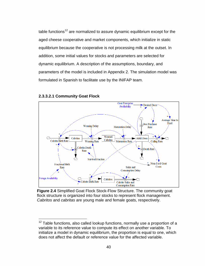
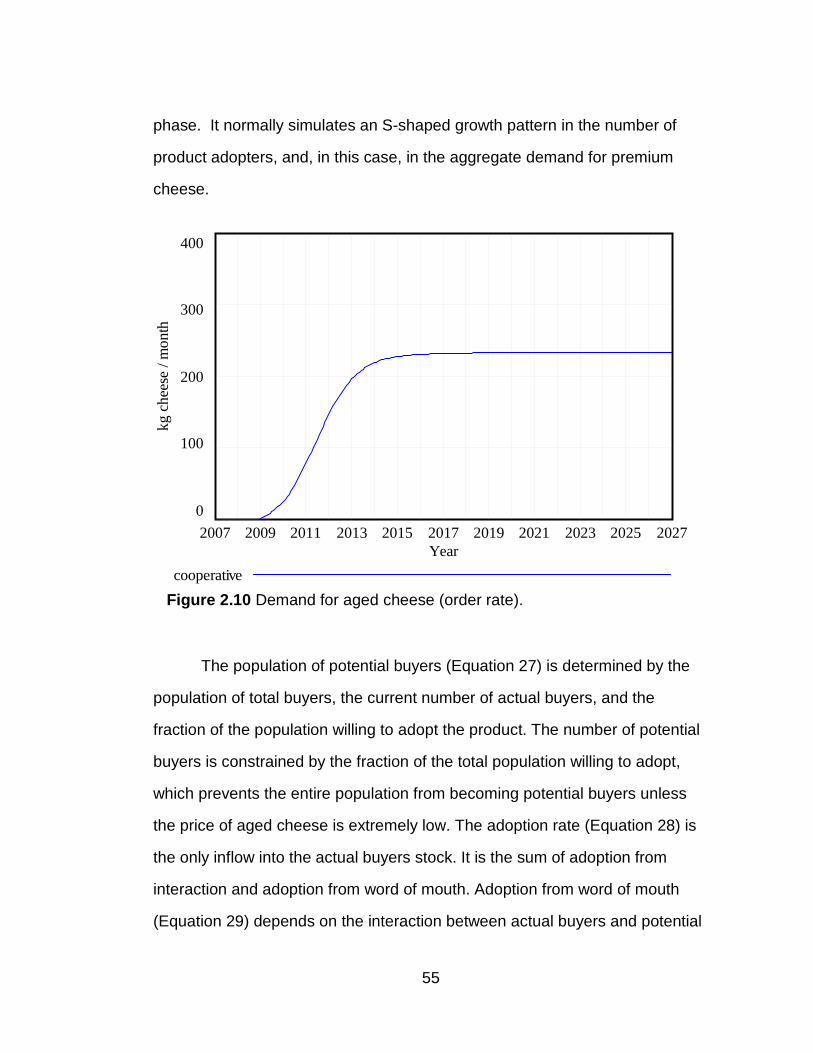
CHAPTER 2: METHODS ............................................................................... 11 2.1 Introduction to System Dynamics ................................................... 11 2.1.1 System Dynamics Modeling ....................................................... 12 2.1.2 System Dynamics Perspective ................................................... 14 2.1.3 Dynamic Modeling Critiques ....................................................... 16 2.1.4 Group Model Building ................................................................. 18 2.1.5 Quantitative versus Qualitative System Dynamics ...................... 20 2.1.6 System Dynamics Modeling Process .......................................... 21 2.2 Professional Short Course on System Dynamics .......................... 23 2.2.1 Course Objectives ...................................................................... 24 2.2.2 Course Location .......................................................................... 24 2.2.3 Course Equipment, Supplies and Learning Materials ................. 25 2.2.4 Course Participants .................................................................... 25 2.2.5 Course Structure ......................................................................... 25 2.3 Value-Added Cooperative Model ..................................................... 28 2.3.0.1 Model History ..................................................................... 28 2.3.0.2 Micoxtla Background .......................................................... 29 2.3.0.3 Micoxtla Economic Activities .............................................. 30 2.3.1 Problem Description ................................................................... 31 2.3.1.1 Reference Mode ................................................................. 32 2.3.1.2 Model Purpose ................................................................... 34 2.3.2 Model Conceptualization ............................................................ 35
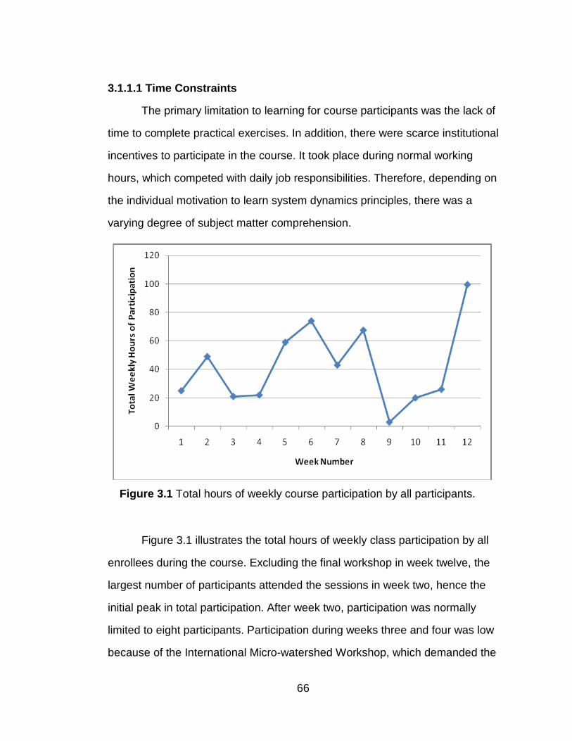
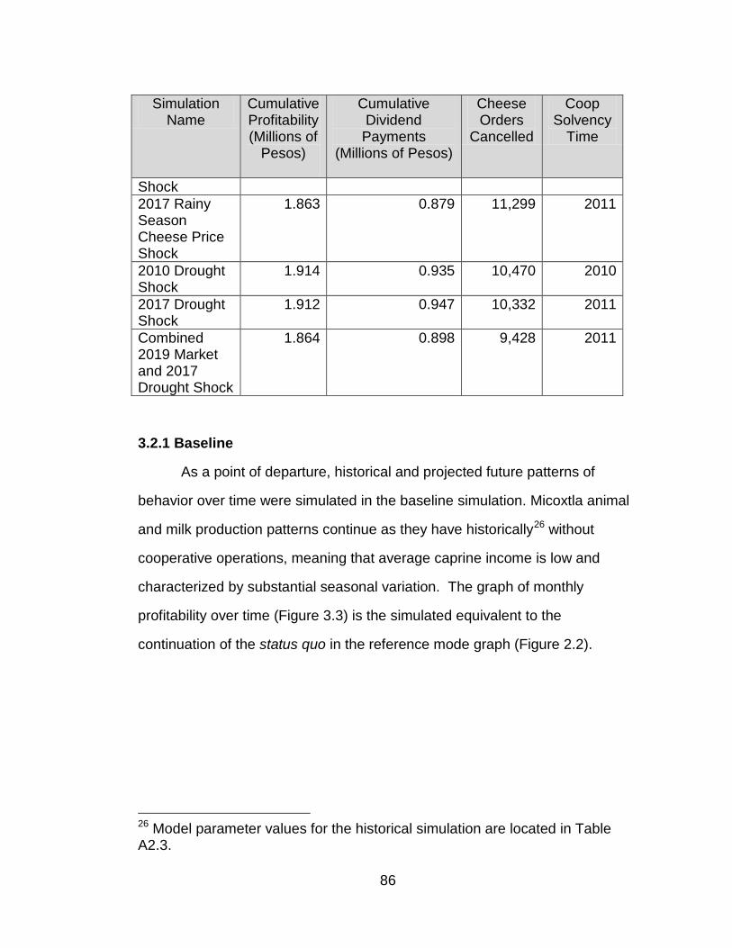
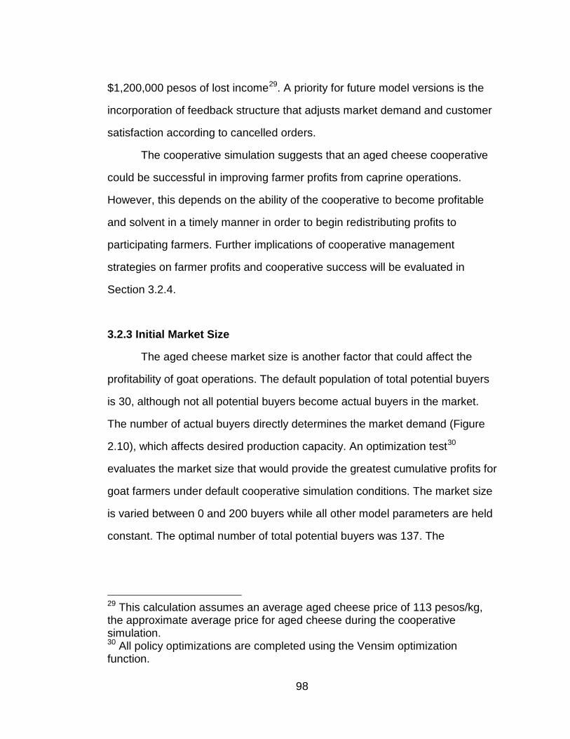
CHAPTER 3: RESULTS AND DISCUSSION ................................................ 64 3.1 System Dynamics Short Course Summary .................................... 64 3.1.1 Short Course Evaluation ............................................................. 65 3.1.1.1 Time Constraints ................................................................ 66 3.1.1.2 Interpretation of System Dynamics Principles .................... 67 3.1.1.3 Behavior Over Time ........................................................... 68 3.1.1.4 Vensim PLE® Software ...................................................... 69 3.1.1.5 Model Formulation .............................................................. 69 3.1.1.6 Spatial Limitations .............................................................. 70 3.1.1.7 Contrasting Methods .......................................................... 71 3.1.1.8 Changes in Problem Conceptualization ............................. 73 3.1.2 Potential Contributions of System Dynamics Methods to Existing INIFAP Programs .......................................................... 77 3.1.3 Team Model Building Case Studies ............................................ 79 3.1.3.1 Diversified Coffee Plantation Team .................................... 81 3.1.4 INIFAP Feedback on Smallholders Value-Added Cooperative Model ......................................................................................... 82 3.2 Value-Added Cooperative Model Policy Analyses ......................... 84 3.2.1 Baseline ...................................................................................... 86 3.2.2 Cheese Cooperative Feasibility .................................................. 89 3.2.3 Initial Market Size ....................................................................... 98 3.2.4 Cheese Cooperative Management ........................................... 102 3.2.4.1 Cooperative Raw Milk Payment Strategies ...................... 103 3.2.4.2 No Dividend Payments ..................................................... 108 3.2.5 Market and Production Shocks ................................................. 111 3.2.5.1 Market Shock ................................................................... 111 3.2.5.2 Below-Average Precipitation Shock ................................. 115
ix
3.2.5.3 Combined Market and Below-Average Precipitation Shocks ............................................................................. 121 3.2.6 Cooperative Sensitivity Tests.................................................... 122 3.2.7 Final Discussion ........................................................................ 128
CHAPTER 4: CONCLUSIONS .................................................................... 132 4.1 System Dynamics Short Course for INIFAP ................................. 132 4.1.1 Interdisciplinary Advantages ..................................................... 134 4.1.2 Group Model Building ............................................................... 135 4.1.3 Ex ante Impact Assessments with System Dynamics ............... 136 4.1.4 Benefits of System Dynamics for INIFAP ................................. 136 4.2 Value-Added Cooperative Model ................................................... 137 4.2.1 Value Addition to Agricultural Products ..................................... 137 4.2.2 Smallholder Value Addition and Marketing Cooperatives ......... 138 4.2.3 Information Needs and Next Steps ........................................... 139 4.3 Personal Reflections ....................................................................... 140
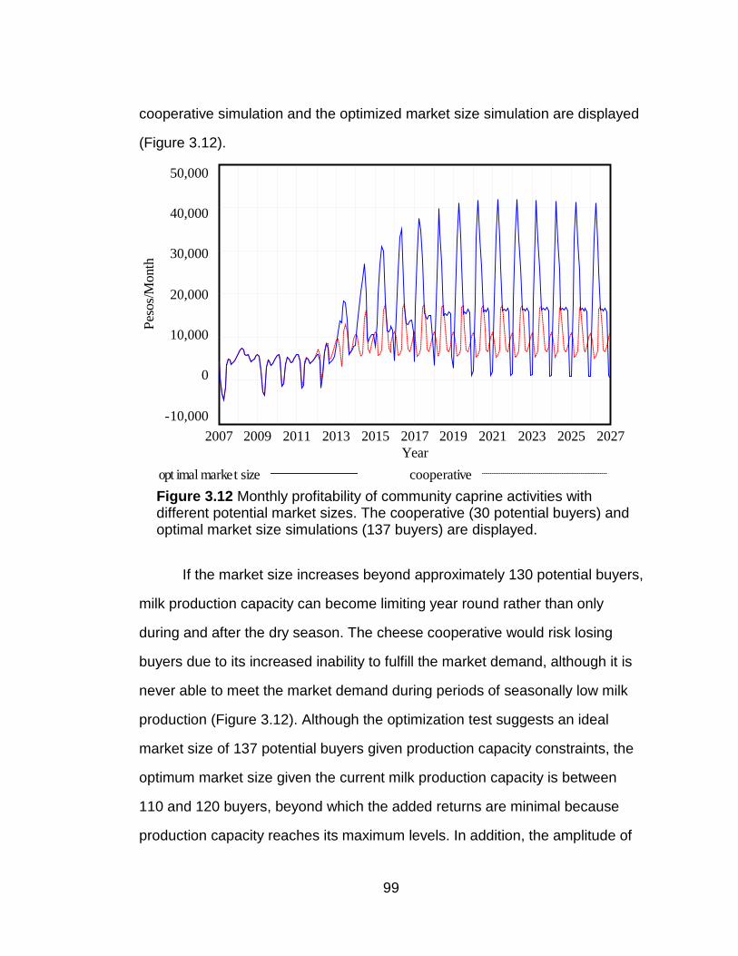
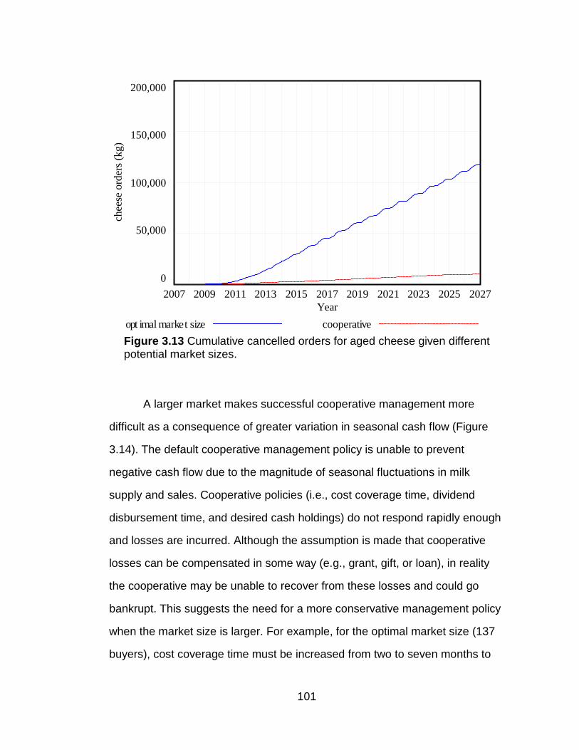
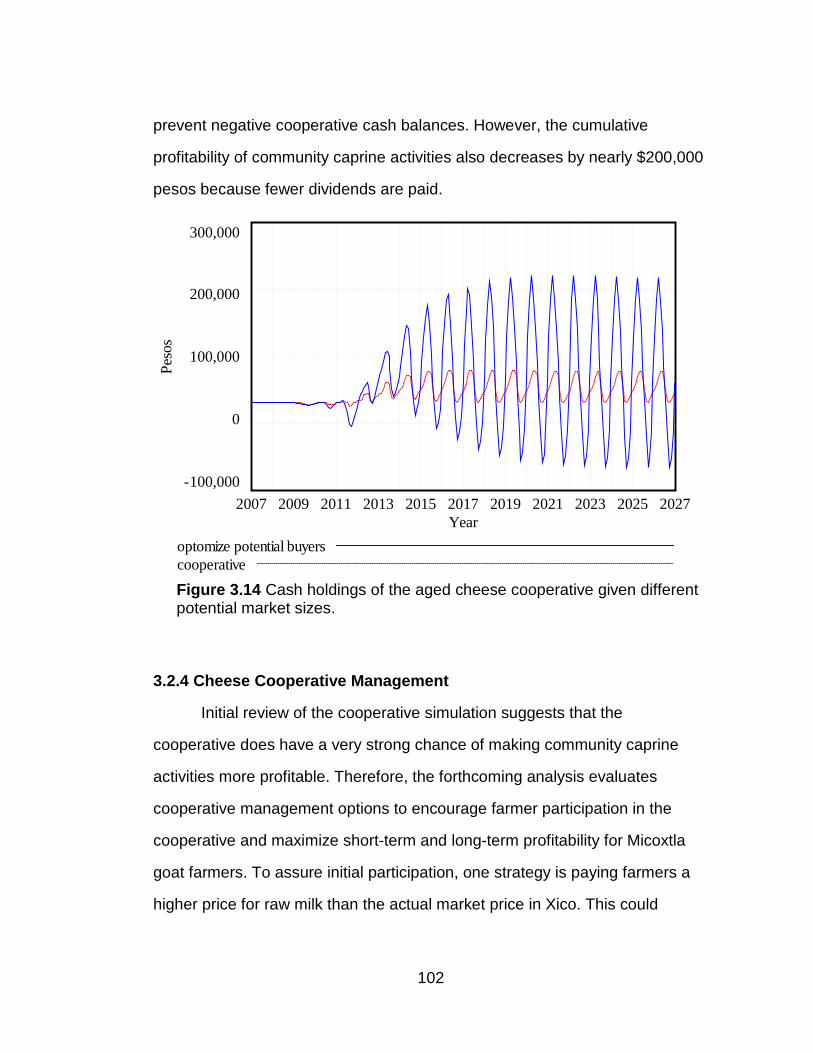
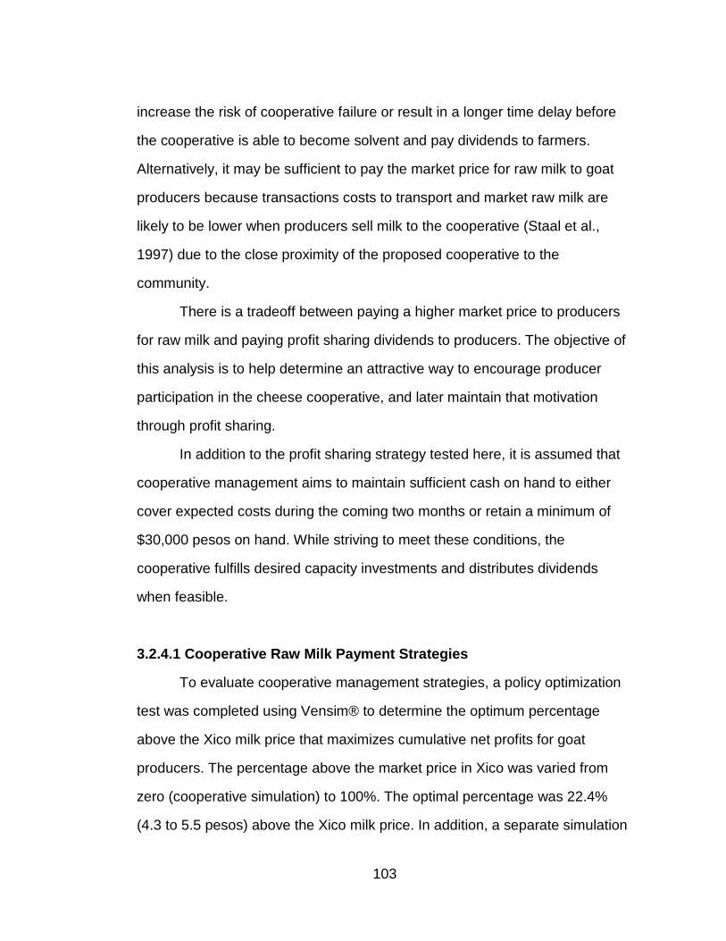
Figure 3.10 Simulated cash holdings of the aged cheese cooperative in the cooperative simulation ...................................................... 96 Figure 3.11 Cumulative cancelled orders for aged cheese, cooperative simulation ................................................................ 97 Figure 3.12 Simulated monthly profitability of community caprine activities with different potential market sizes for aged cheese ................. 99 Figure 3.13 Simulated cumulative cancelled orders for aged cheese given different potential market sizes ....................................... 101 Figure 3.14 Simulated cash holdings of the aged cheese cooperative given different potential market sizes ....................................... 102 Figure 3.15 Simulated monthly profitability of community caprine activities with different milk payment strategies ........... 104 Figure 3.16 Simulated monthly dividend payments with different milk payment strategies ...................................... 106
xi
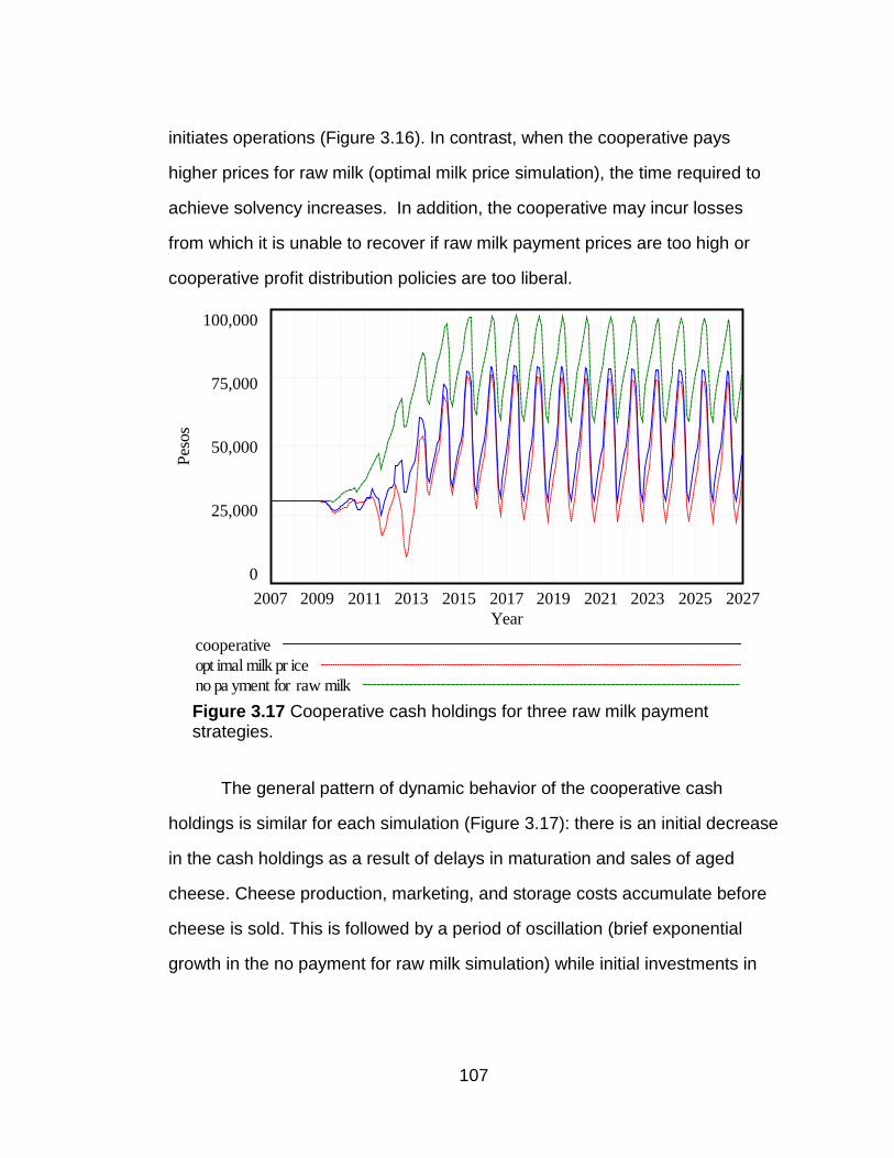
Figure 3.17 Simulated cooperative cash holdings given three different payment strategies for raw milk ................................................ 107
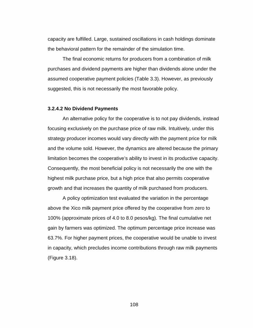
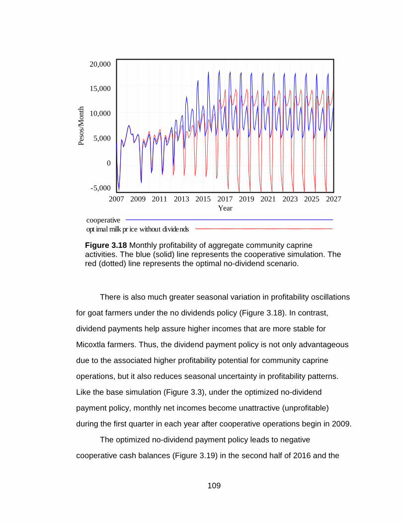
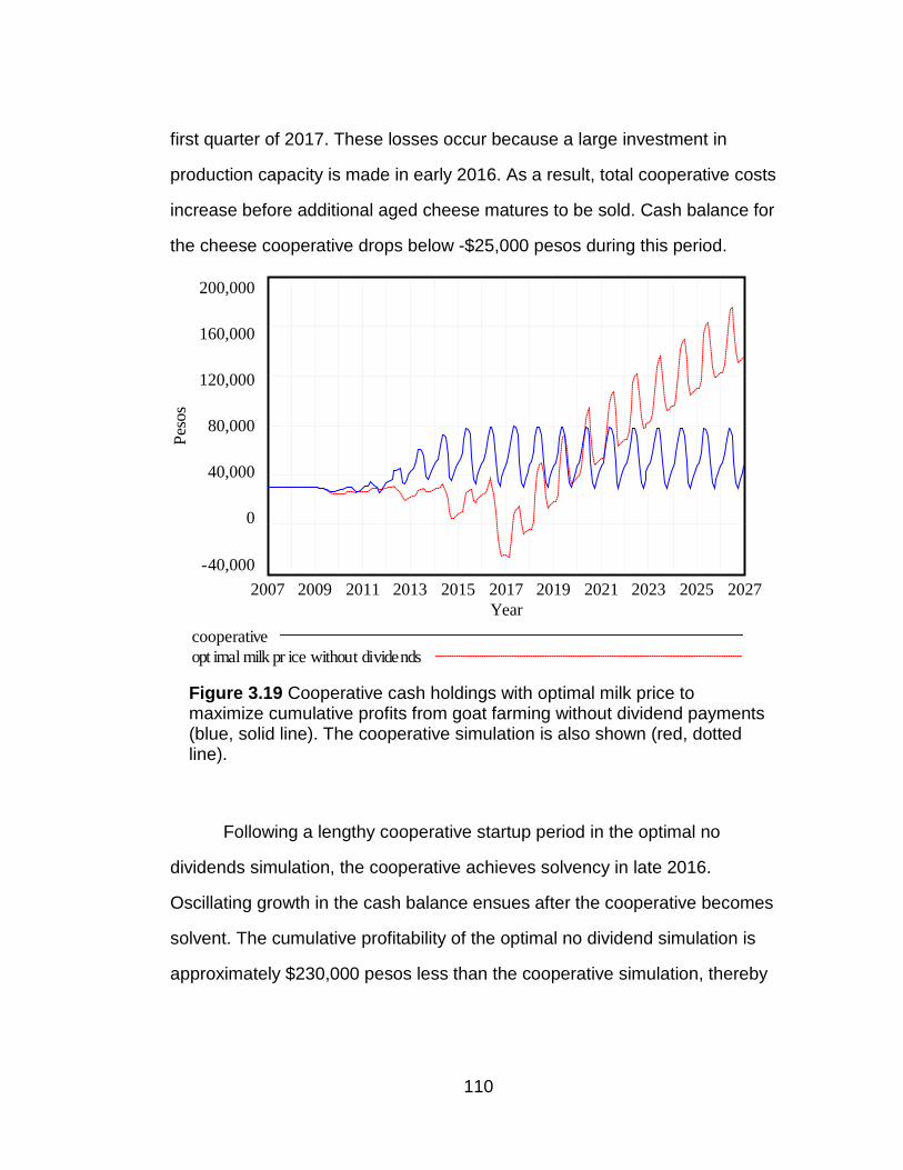
Figure 3.18 Simulated monthly profitability of aggregate community caprine activities, optimized no dividend scenario. ................... 109 Figure 3.19 Cooperative cash holdings with optimal milk price to maximize cumulative profits from goat farming without dividend payments ................................................................... 110 Figure 3.20 Simulated monthly profitability of aggregate community
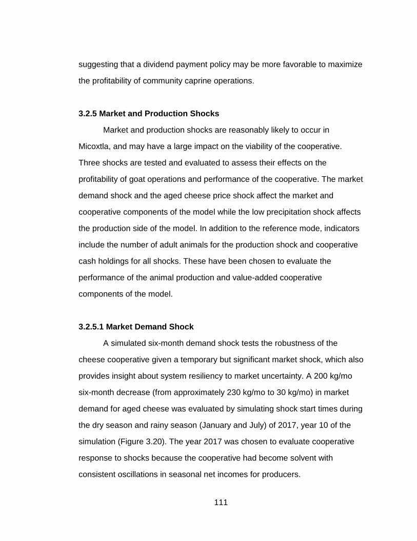
caprine operations with 2017 dry and rainy season demand shocks. ....................................................................... 112
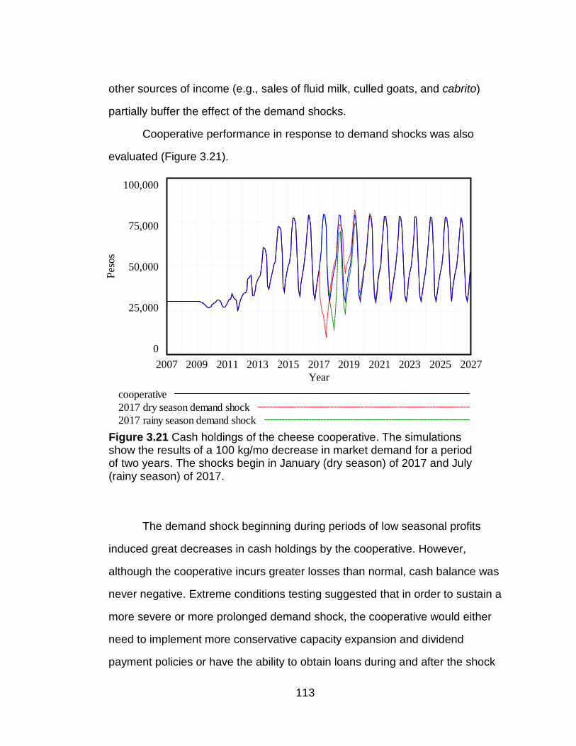
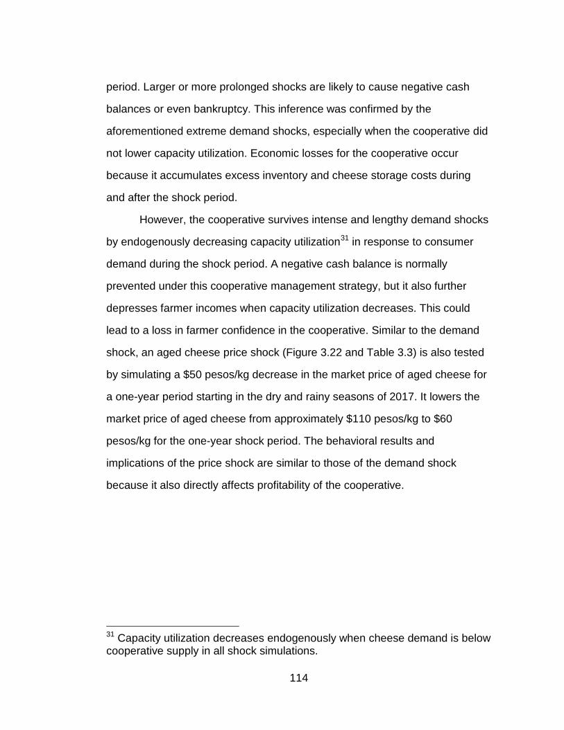
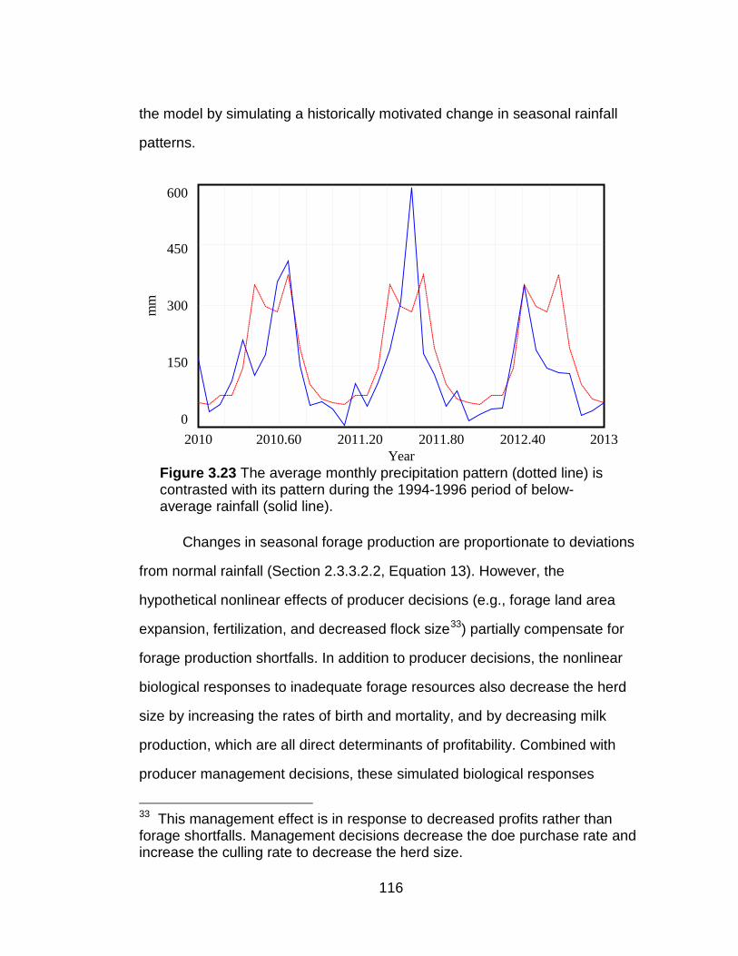
Figure 3.21 Simulated cash holdings of the cheese cooperative with 2017 dry and rainy season demand shocks ...................... 113 Figure 3.22 Simulated monthly profitability of community caprine operations with 2017 dry and rainy season price shocks ......... 115 Figure 3.23 The average monthly precipitation pattern is contrasted with the precipitation pattern during the 1994-1996 below-average precipitation shock ........................................... 116 Figure 3.24 Simulated monthly profitability of aggregate community
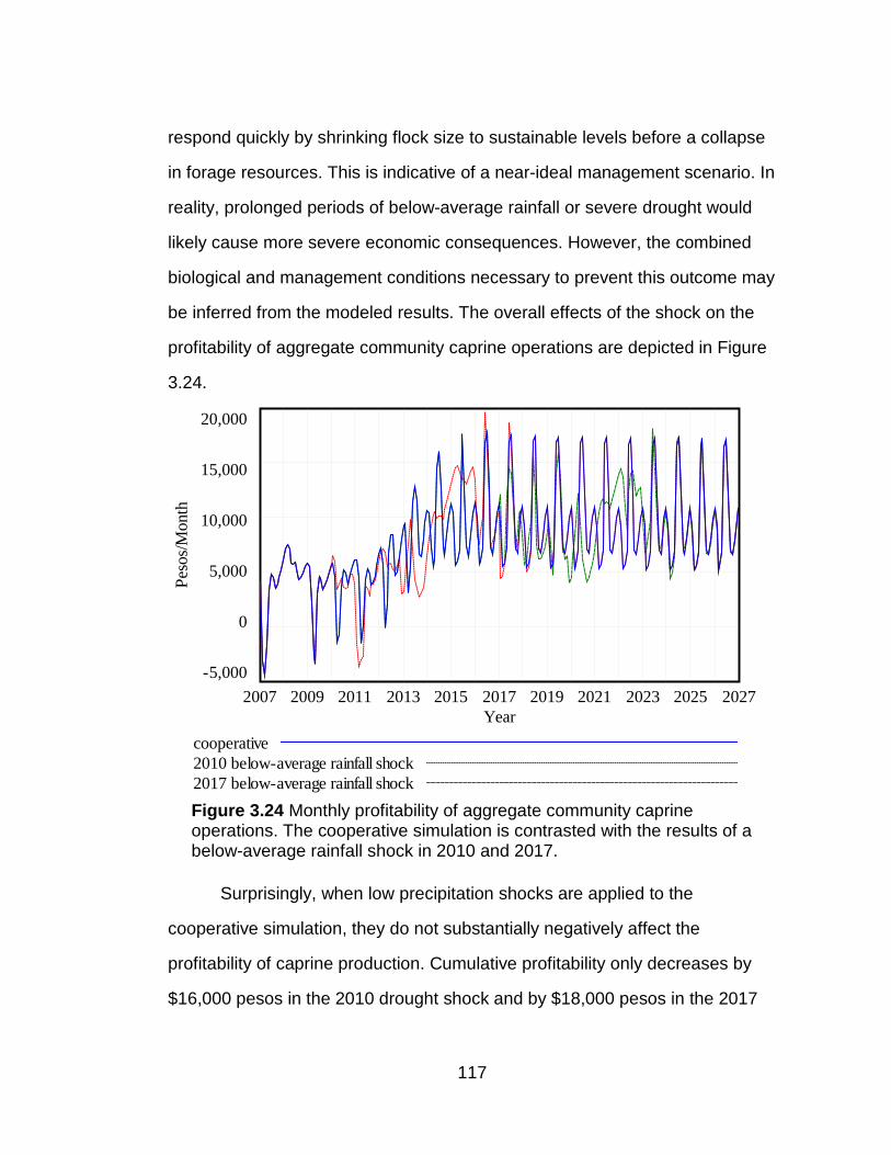
caprine operations with a 2010 and 2017 below-average precipitation shock .................................................................... 117
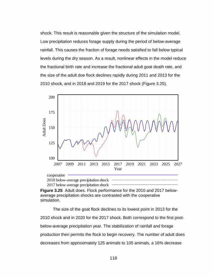
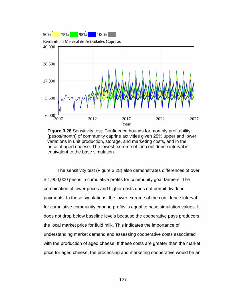
Figure 3.25 Simulated adult does, flock performance for the 2010 and 2017 below-average precipitation shocks................. 118 Figure 3.26 Simulated cheese cooperative cash holdings with 2010 and 2017 below-average precipitation shocks................. 120 Figure 3.27 Simulated monthly profitability of aggregate community caprine operations with combined market and below-average precipitation shocks ......................................... 121 Figure 3.28 Sensitivity test for cheese costs and price ................................ 127
xii
LIST OF TABLES
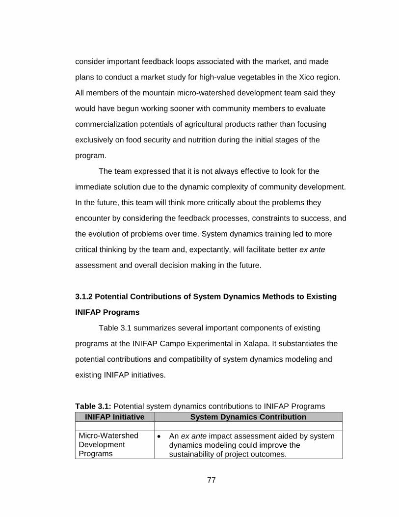
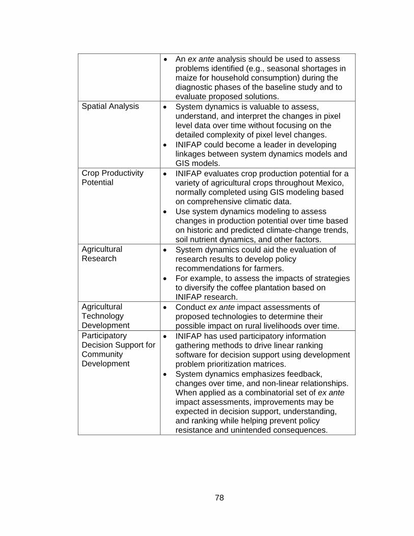
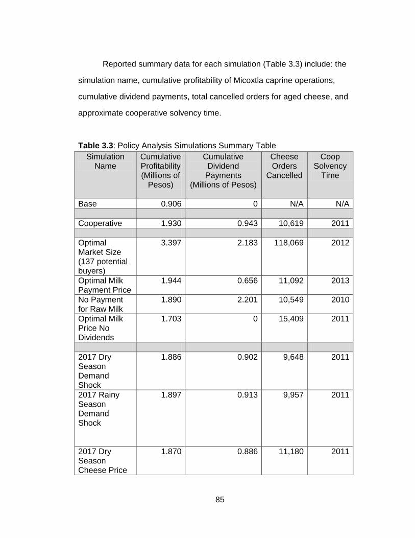
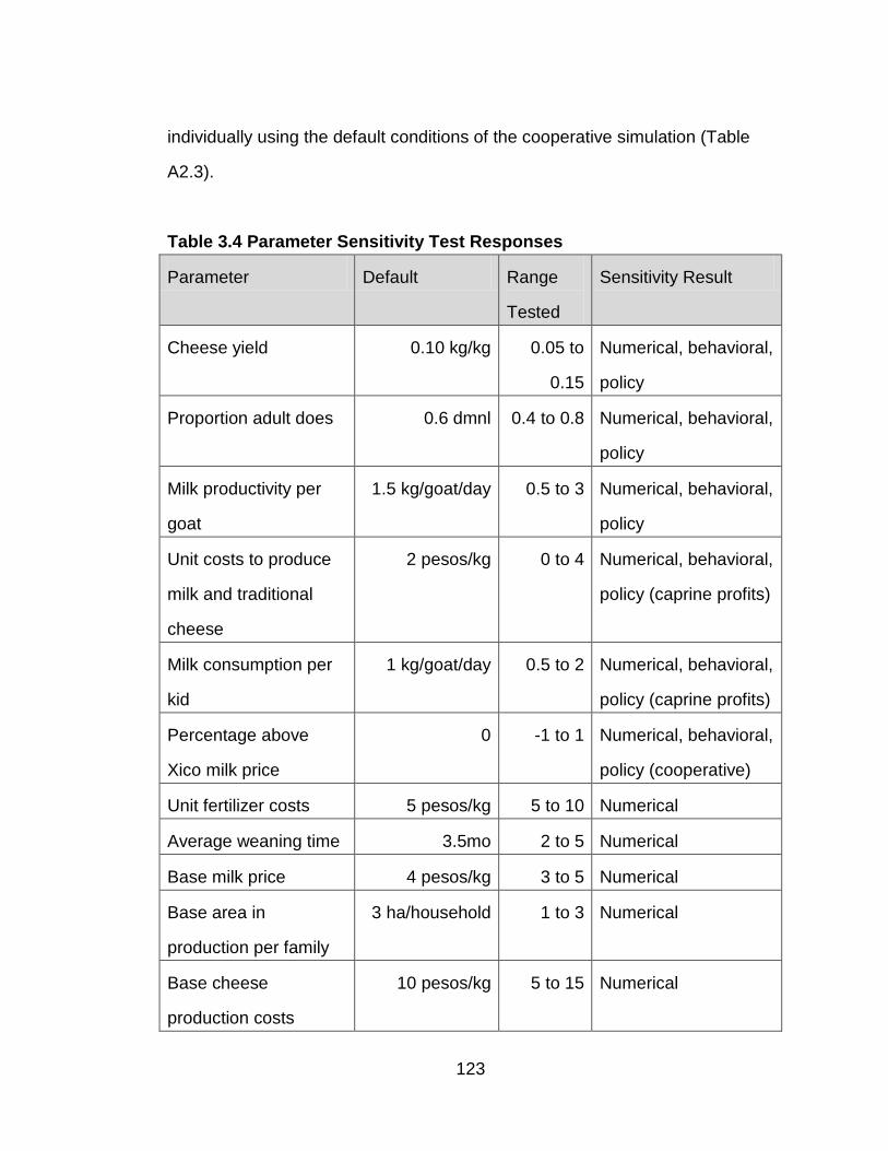
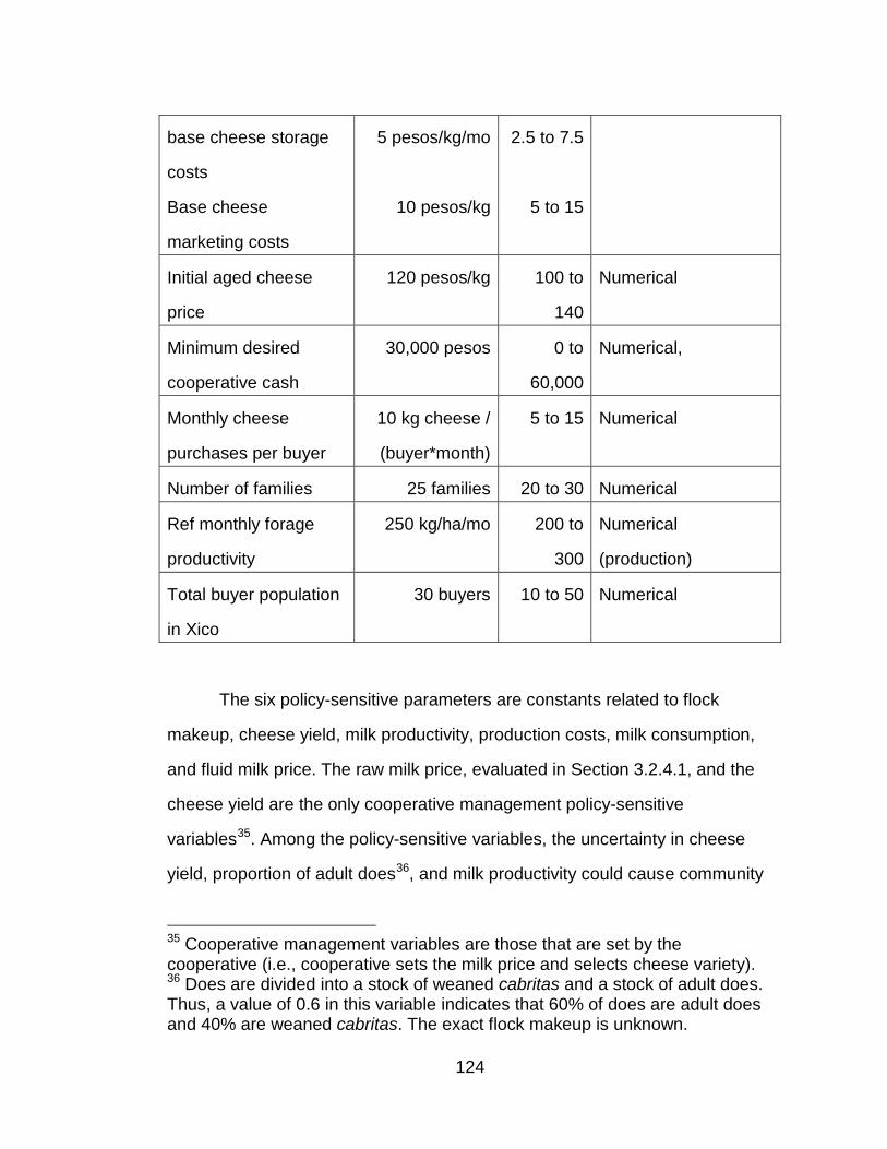
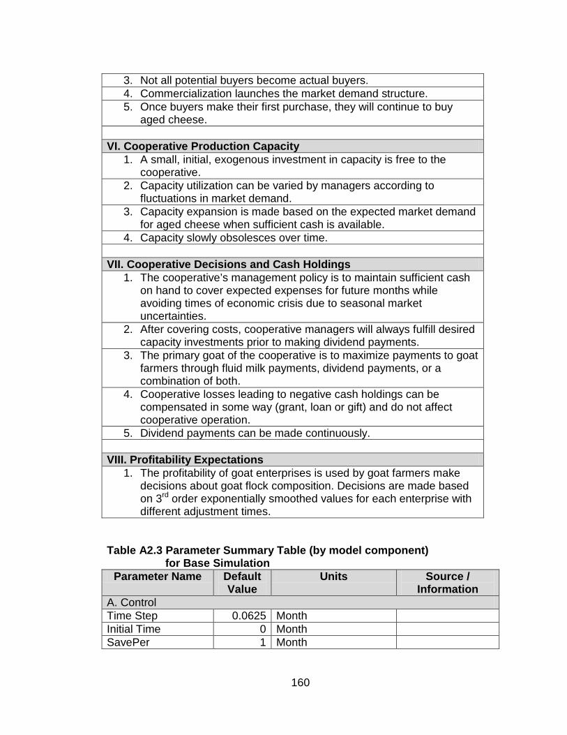
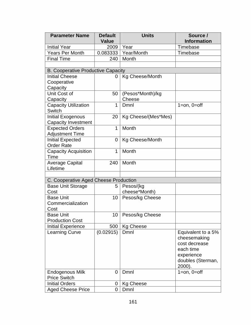
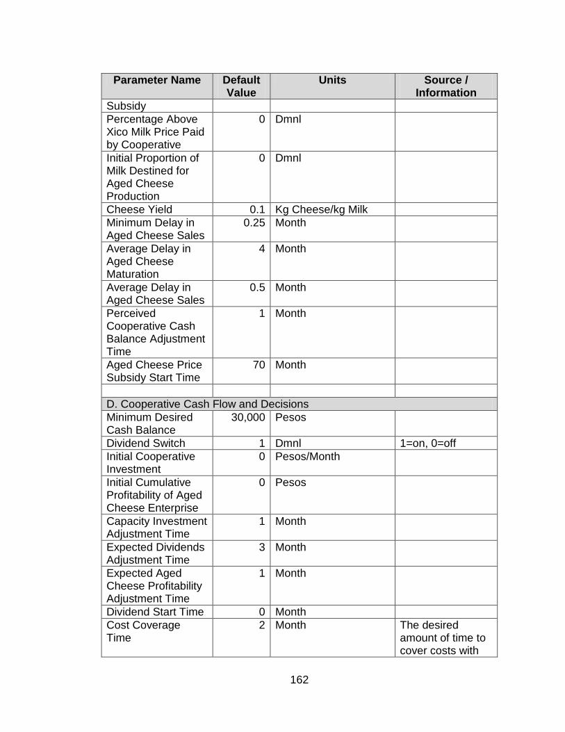
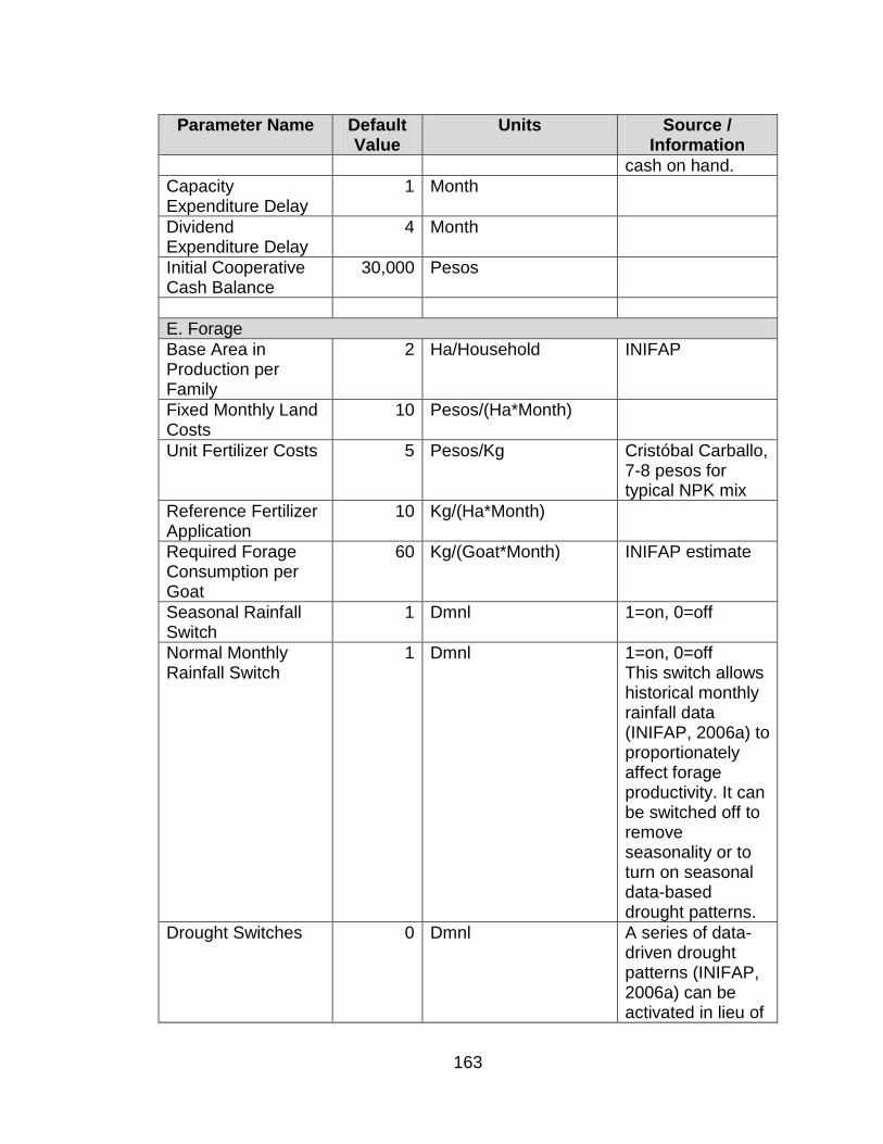
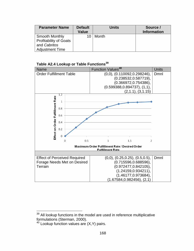
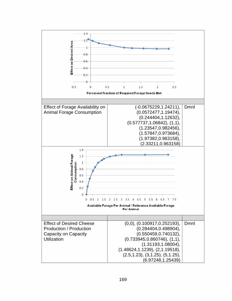
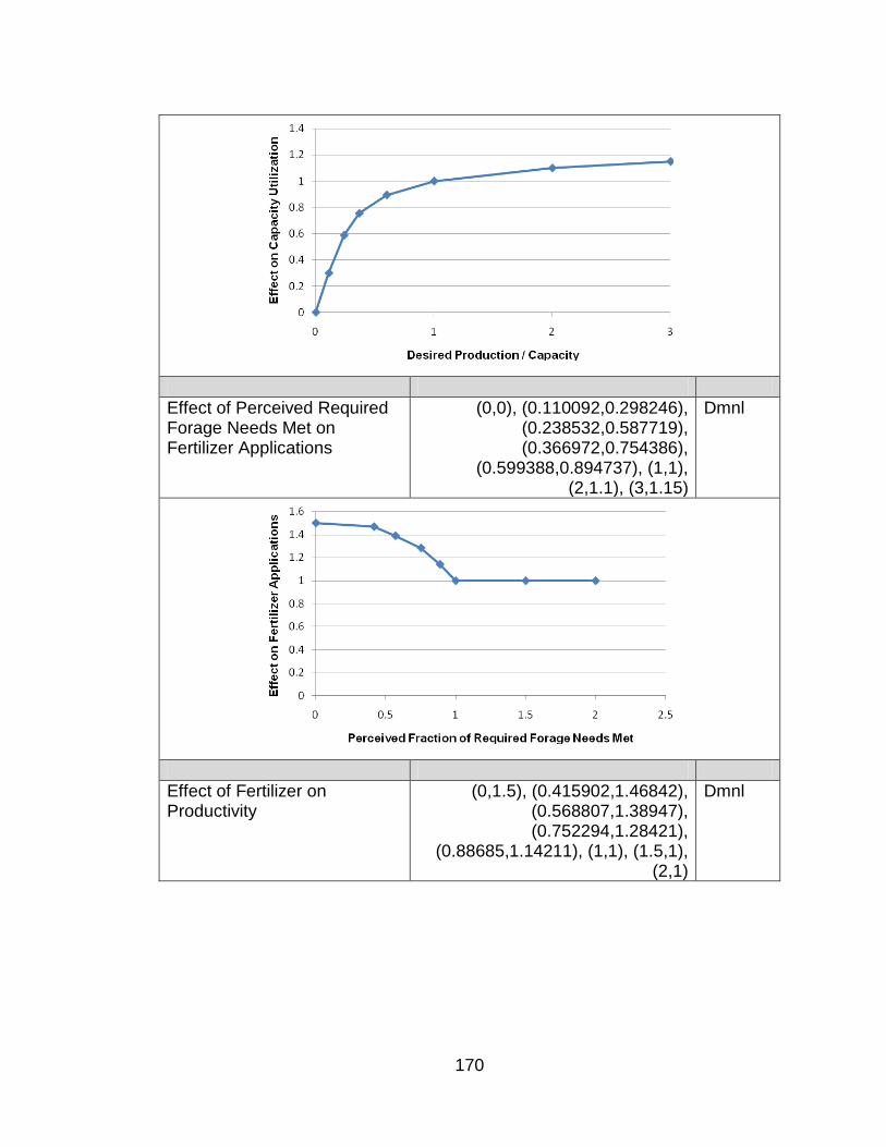
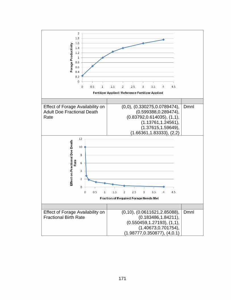
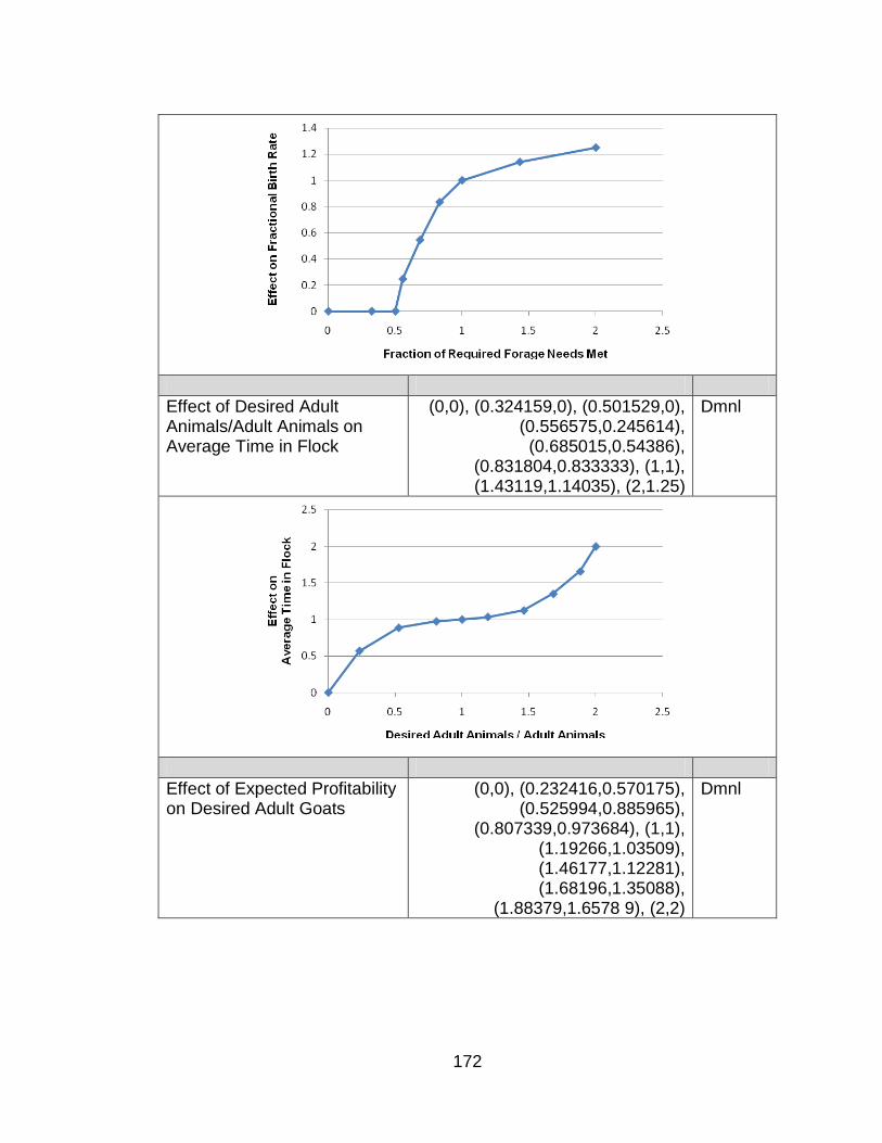
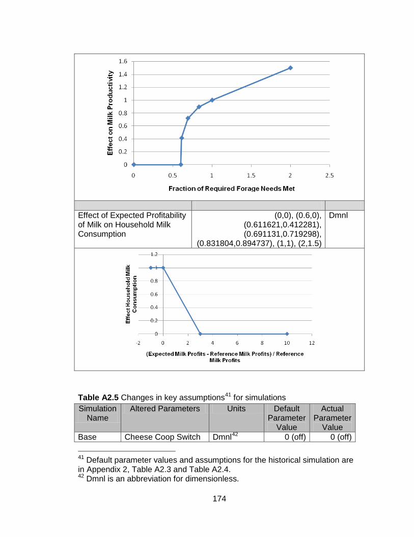
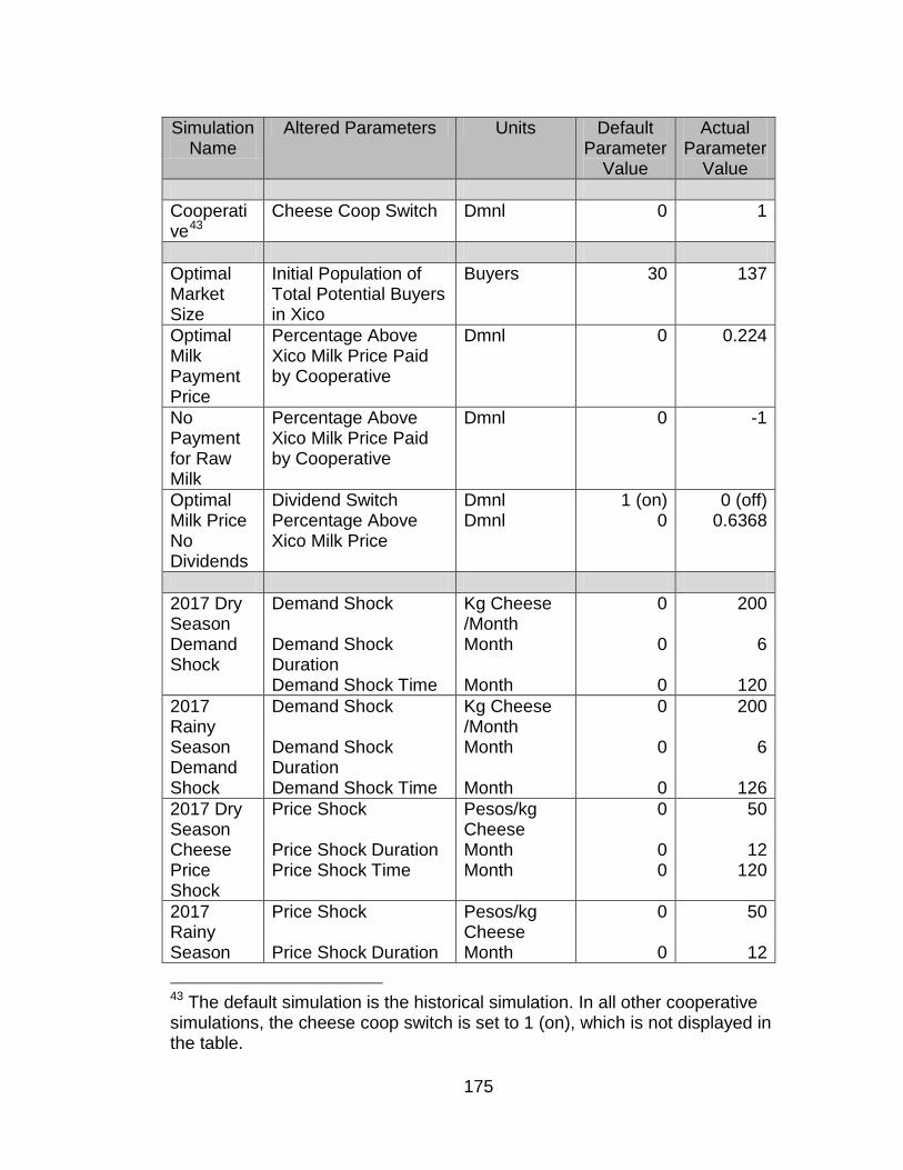
Table 3.1 Potential Contributions of System Dynamics to INIFAP Programs . 77Table 3.2 INIFAP Suggestions and Comments on Preliminary Model ........... 83 Table 3.3 Policy Analysis Simulations Summary Table .................................. 85 Table 3.4 Parameter Sensitivity Test Responses ......................................... 123 Table A2.1 Model Boundary Table ............................................................... 157 Table A2.2 Model Assumptions .................................................................... 158 Table A2.3 Parameter Summary Table for Base Coop Simulation ............... 160 Table A2.4 Model Lookup or Table Functions .............................................. 168 Table A2.5 Changes in Key Assumptions for Policy Analysis Simulations ... 174 Table A2.6 Seasonal Rainfall Data at Teocelo, Veracruz ............................. 176
xiii
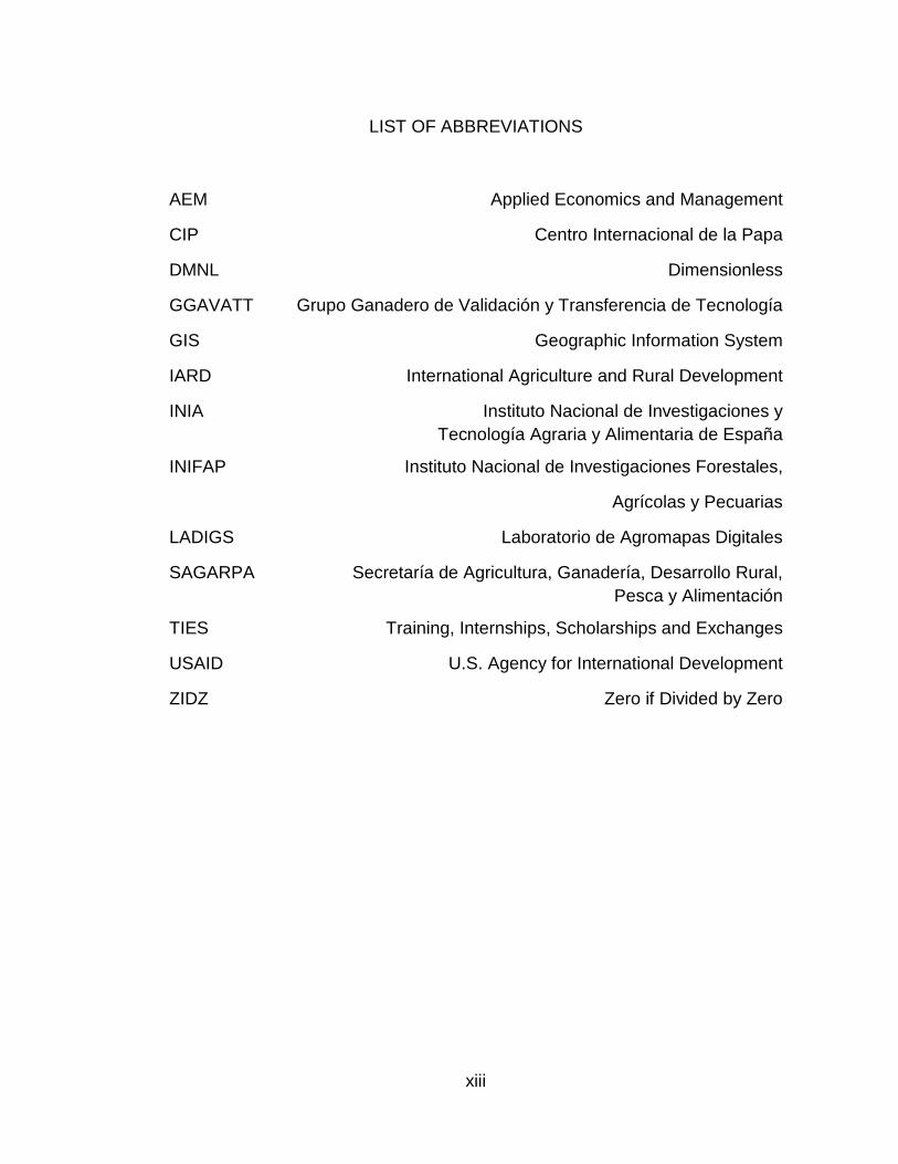
LIST OF ABBREVIATIONS
AEM Applied Economics and Management
CIP Centro Internacional de la Papa
DMNL Dimensionless
GGAVATT Grupo Ganadero de Validación y Transferencia de Tecnología
GIS Geographic Information System
IARD International Agriculture and Rural Development
INIA Instituto Nacional de Investigaciones y Tecnología Agraria y Alimentaria de España
INIFAP Instituto Nacional de Investigaciones Forestales,
Agrícolas y Pecuarias
LADIGS Laboratorio de Agromapas Digitales
SAGARPA Secretaría de Agricultura, Ganadería, Desarrollo Rural, Pesca y Alimentación
TIES Training, Internships, Scholarships and Exchanges
USAID U.S. Agency for International Development
ZIDZ Zero if Divided by Zero
xiv
PREFACE
This project had its origin in the author’s experience working with rural
communities and numerous governmental and non-governmental
organizations as a Peace Corps Volunteer and Peace Corps Technical Trainer
in Nicaragua. Upon arrival at Cornell University he had a strong desire to
undertake a practical project that could contribute to an international
organization or to a community in Latin America. His goal was to achieve more
than just earning a degree, but also to contribute with capacity building
assistance at the request of an organization or a community.
The opportunity emerged when the author began to work with the multi-
institutional Training, Internships, Exchanges and Scholarships (TIES) Mexico
project, Decision Support of Ruminant Livestock Systems in the Gulf Region of
Mexico. The decision to focus on system dynamics applications was made
during his first semester at Cornell when he was introduced to the use of
system dynamics for agricultural development during the Applied Economics
and Management (AEM) 494 course, Introduction to System Dynamics
Modeling. The course provided evidence and motivation for creating a system
dynamics platform for critical thinking in a rural development forum. The author
simultaneously enrolled in a two-course package, International Agriculture and
Rural Development (IARD) 402/602 Mexico, and participated in the IARD 602
field laboratory in Mexico in January 2007. During the two-week field
experience in Mexico, he became acquainted with TIES collaborator Gabriel
Díaz Padilla and the rest of the Instituto Nacional de Investigaciones
Forestales, Agrícolas y Pecuarias (INIFAP) mountain research team in
xv
Xalapa, Veracruz, with whom the foundation for future collaboration was
established.
Background about INIFAP
INIFAP is a Mexican governmental institution dedicated to research and
development of agricultural technologies. The INIFAP office in Xalapa,
Veracruz is the administrative base for numerous agricultural research
programs. Its Campo Experimental in Teocelo focuses on the viability of
different methods of diversifying the traditional coffee plantation by planting in
association with timber species, ornamental plants, and silvopastoral systems
with sheep. In a separate INIFAP project led by the Laboratorio de Agromapas
Digitales (LADIGS), the Campo Experimental is among the Mexican leaders in
spatial modeling of crop production potential using Global Information Systems
(GIS) methods. LADIGS also develops regional maps of historical and
projected climatic trends.
The Campo Experimental executed a mountain micro-watershed
development project from 2003 to 2008. Different from most INIFAP programs
and the institution’s mandate, community development and extension were
important components of this project. Funding for the micro-watershed project
was provided by the Instituto Nacional de Investigaciones y Tecnología
Agraria y Alimentaria de España (INIA) and implemented collectively by
INIFAP and the Centro Internacional de la Papa (CIP). The project was
designed to develop technology and agricultural alternatives that will improve
sustainable management of key micro-watersheds while raising the standard
of living in participating communities. It focused on four branches of rural
development: agronomic, economic, health, and socio-cultural development
xvi
(Díaz Padilla et al., 2006). Key activities in the project included: low-cost basic
infrastructure (e.g., high efficiency wood stoves, compost latrines, and
greenhouses), integrated patio management, family health and nutrition,
ruminant livestock production, improved forages, and staple grains
management. These components were jointly selected by INIFAP personnel
and members of three communities—Micoxtla, Mesa de Laurel, and Ingenio
del Rosario—during the diagnostic phase of the project in 2003.
Similar projects were concurrently led by Díaz Padilla in priority
watersheds in the states of Durango and Chiapas. The three watersheds were
selected based on common problems: unemployment, low incomes,
environmental degradation, and food insecurity (Díaz Padilla et al., 2006). As
of January 2008, INIFAP’s watershed work in Veracruz was undergoing a
transition toward intensive micro-watershed investigation to improve water
management in the Gavilanes River (Coatepec) micro-watershed.
INIFAP/Cornell University Collaboration
The INIFAP Campo Experimental in Xalapa, Veracruz collaborated with
Cornell University on the United States Agency for International Development
(USAID) Training, Internships, Exchanges and Scholarships (TIES) Mexico
initiative. As part of the TIES program, Gabriel Díaz Padilla attended Cornell
for a semester-long sabbatical in 2005. During that time, he was introduced to
systems science applications and dynamic modeling during the introductory
system dynamics course. The sabbatical generated further interest for INIFAP
researchers and technicians to collaborate with Cornell University.
Later, INIFAP helped organize and received three study groups
comprising students and faculty from Cornell University, the Universidad
xvii
Veracruzana, and the Universidad Autónoma de Yucatán during the IARD
602-Mexico field courses in 2006, 2007, and 2008. The author was a
participant and then a facilitator during the field courses in 2007 and 2008.
Following the 2007 field trip, he worked with Díaz Padilla and advisors Robert
Blake, Charles Nicholson, and Terry Tucker to explore options for coordinated
field research with the INIFAP team.
INIFAP suggested the need to further develop agricultural value-
addition components of their mountain project. One of the more important
income generation activities in Veracruz highlands communities is the sale of
goat’s milk. However, low profits suggested a potential need to explore options
to derive high-value products from the milk produced. This priority option, also
identified by community members, became a master example for the author’s
exploratory system dynamics work during a second course in system
dynamics applications (AEM 700). In this course, a preliminary model
addressing value addition to goat’s milk by cheese manufacture was
developed as a tool for pedagogical and analytical purposes in preparation for
summer 2007 field activities with INIFAP in Xalapa, Veracruz.
The INIFAP team also expressed interest in receiving a course on
systems thinking and modeling using system dynamics methods. At their
request, the author taught an introductory system dynamics course in Xalapa.
The three-month course, conducted from June to September 2007, was titled,
Introducción al Pensamiento Sistémico y Modelación Dinámica de Problemas
(Introduction to Systems Thinking and Dynamic Problem Modeling). This
course emulated the system dynamics curriculum at Cornell University. It
provided INIFAP with valuable learning and insight about potential agricultural
and rural development applications of system dynamics. The course fulfilled
xviii
the desired institutional capacity building component of the author’s master’s
project. Based on INIFAP’s institutional goals and participant interests, team
model building activities were undertaken as an important course component.
The timeline trajectory to thesis project completion is described below:
2006
• August: The author initiated graduate studies at Cornell University and
enrolled in Introductory System Dynamics.
2007
• January: Possibilities for a collaborative thesis research project with
INIFAP were explored during the IARD 602-Mexico field course.
• February: The author was awarded a summer travel grant from the
Latin American Studies Program to initiate thesis activities in Mexico.
• February to May: The author enrolled in System Dynamics Applications.
Based on INIFAP feedback, thesis advisor recommendations, and
author interest, the economic feasibility of value-added dairy products
(aged cheeses) was selected for the development of a preliminary
system dynamics model. The preliminary model was developed and
initial baseline simulations were conducted.
• May: INIFAP extended an invitation for an introductory systems thinking
and dynamic modeling course in Xalapa, Veracruz. Instructional
materials were developed to integrate the course with parallel learning
activities for the development of this thesis.
• June to September: The three-month introductory system dynamics
course was taught for INIFAP in Xalapa, Veracruz. Group model
xix
building exercises were integrated in response to INIFAP’s request.
Participants included INIFAP research and extension workers and a
University of Veracruz student in economics.
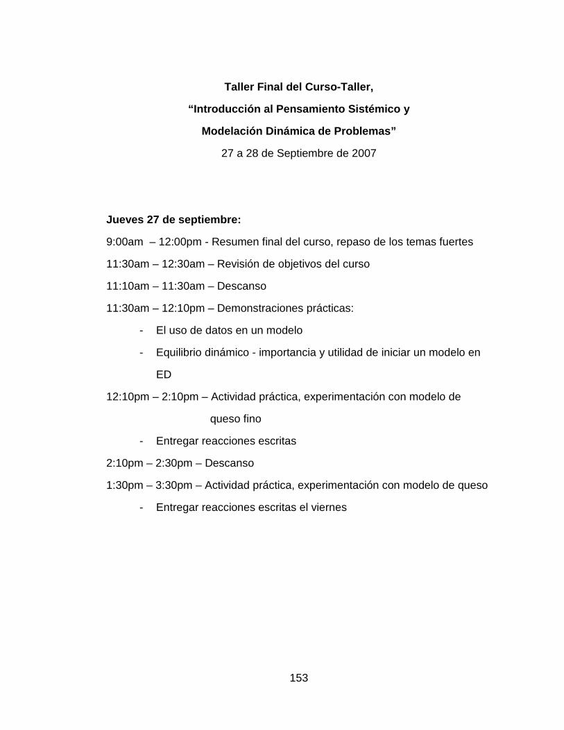
• July: The author presented Alternativas Económicas en Microcuencas
de Montaña: Potencial del Queso Añejo de Cabra at the International
Workshop on Mountain Microwatershed Management in Xalapa.
2008
• January: The author worked as a field-learning facilitator in the IARD
602 course involving participatory rural appraisal workshops in two
mountain communities, Cuatitlan and Xico Viejo, near Xico, Veracruz.
After these workshops, follow-up activities from the introductory system
dynamics course were completed with the INIFAP team.
From August 2007 to June 2008, the author also served as an informal
advisor to Martín Alfonso López Rámirez, a student at the University of
Veracruz in Xalapa for the system dynamics component of his undergraduate
thesis in economics. This thesis, Diversificación Productiva de Cafetales: Un
análisis de riesgo y rentabilidad mediante la aplicación de Dinámica de
Sistemas (López Ramírez, 2008), was completed using the system dynamics
methods taught in the introductory system dynamics course.
1
CHAPTER 1
INTRODUCTION
Mexico is a country of economic extremes. The wealthier northern
states contrast with widespread poverty in southern states (Aguirre Reveles
and Sandoval Terán, 2001). In the southern state of Veracruz, agriculture-
based rural communities struggle with food insecurity, unemployment, and
variable agricultural incomes. Market uncertainties often limit economic
development opportunities in these rural communities. Poverty alleviation in
these regions is contingent on improving food security and achieving rural
economic growth (Blake, 2003). Specifically, an important component of
poverty reduction is the generation of income opportunities for poor rural
families. The generation of income opportunities can be achieved by
producing high-value products with competitive advantages in local and
regional markets. These products, especially when manufactured and
marketed by local farmer collectives or cooperatives, have the potential to
dramatically improve rural livelihoods through greater profitability from
agriculture.
Multiple governmental and non-governmental organizations invest
human and financial capital in poverty alleviation initiatives. There is a need to
coordinate these efforts to improve the efficacy, impact, and potential for more
widespread dissemination of successful interventions. This study aims to
foster multi-institutional collaboration by implementing system dynamics
methodology as a platform to encourage critical thinking, teamwork,
information sharing, and improved policies in the analysis of complex, dynamic
agricultural problems. To achieve this overall goal, group model building using
2
system dynamics methods to conduct ex ante or preliminary assessment of
these complex agricultural problems can be advantageous. Thus, the ex ante
assessment of several problems encourages system dynamics learning,
improves problem understanding, and ultimately improves decision making for
agricultural research and development initiatives.
1.1 Collective Action for Value Addition and Marketing
To better capitalize on local and regional market potential and market
access while reducing market uncertainty, collective action in the form of rural
cooperatives could help increase household incomes. The production and
marketing of higher-value products could help Veracruz highland communities
generate additional income and become more active in dynamic local and
regional markets. To achieve this outcome, cooperatives could play a
facilitative role by involving local producers and increasing profits from value
addition to products marketed by rural communities.
Small dairy cooperatives have had a positive impact on rural
communities in various parts of the world. For example, in peri-urban locations
of the Ethiopia highlands, the formation of small cooperatives called producer
milk groups was successful in raising the incomes of rural dairy farmers
(Nicholson et al., 1998). These cooperatives provided an alternative market
outlet for fluid milk by purchasing it from farmers and processing it into dairy
products such as cheese and butter. Some cooperatives further increased
incomes of participating dairy farmers by returning profits in the form of
dividends. They have also generated employment for members in rural
communities.
3
In general the primary objective of these dairy cooperatives is to
maximize cash flow to participating farmers, not necessarily to maximize
profits (Nicholson et al., 1998). First, dairy cooperatives can purchase raw milk
for a higher price than the local markets. By offering a higher price for raw
milk, it is easier to encourage farmer participation. However, profits to the
cooperative decrease and the risk of failure is higher, especially during the
startup phase. Second, the dairy cooperatives can offer a lower price for raw
milk, thereby accelerating solvency and increasing their ability to distribute
profits with participating farmers. The profits from processing and sales of
value-added products can be returned to farmers as dividends (Holloway et
al., 1999). Due to the lower milk price, the initial benefits of farmer participation
are less and the perceived risk of participation in the cooperatives is elevated,
but the long-term cash flow to farmers may increase. Additional profits also
allow for further marketing and cooperative capacity investments. A
cooperative management strategy that includes a combination of both higher
prices for raw milk and dividend payments could be especially advantageous
for farmers.
Seasonal changes in milk production quantity and quality, and milk
price and demand trends present a unique set of challenges for producers and
cooperatives. In Honduras and Nicaragua, the quantity of milk produced is
higher during the rainy season, but milk quality suffers and milk prices are
lower (Holmann, 2001). In contrast, during the dry season milk supply
decreases but milk quality is better from more hygienic milking with less
muddy conditions. The superior milk quality combined with supply shortages
render higher market prices.
4
Holloway et al. (1999) also suggested that the distance between market
outlets and production points is highly correlated with milk quality due to
lengthy delivery delays. Closer proximity to milk cooperatives decreases the
distance to market, assuring fresh, higher quality raw milk for processing and
increasing the attractiveness of farmer participation in milk groups due to lower
transactions costs. Therefore, the location of the milk groups provides another
benefit for dairy farmers by lowering these costs (Staal et al., 1997). In the
Coatepec highlands, a value-added cooperative that processes and markets
goat’s milk could increase the profitability of smallholder goat production
operations.
A successful dairy cooperative could provide considerable economic
benefits to farmers while decreasing the time and resources they invest to
market and sell raw milk. As a result, depending on the characteristics of the
cooperative, market access can increase while sources of market uncertainty
decrease.
1.2 Ex ante Problem Analysis
What is being referred to here as an ex ante problem analysis is
commonly termed ex ante impact assessment in the field of international
development. Many impact assessments are conducted ex post during the
monitoring and evaluation phases of past projects. Although ex post
assessments provide insight about what could have been improved,
retrospective leverage points in the system, and reasons for desirable and
undesirable outcomes, they cannot compensate for past shortcomings. In
contrast, ex ante impact assessments evaluate problems, development
programs, policies, and proposed solutions prior to their implementation.
5
These assessments provide insight about future development activities that
can be used to improve planning, decision making, and methodology before
the execution phase.
International development problems, especially those that address
social systems in community development, are often poorly understood, and
interventions have achieved mixed results. Even successful ones have
unintended consequences. Ex ante impact assessments provide greater
insight than expert intuition alone, thereby improving understanding in these
complex systems (Sterman, 2006). There is great need for ex ante
assessments to define leverage points, key variables, information needs, and
critical conditions for the success of programs and problems. To develop an
effective ex ante impact assessment, it is vital to attain a high level of
understanding about the dynamically complex problem. This is especially
critical in the often poorly understood, complex, multifaceted agriculture-based
livelihoods of economically poor rural areas in developing countries (Thornton
et al., 2003).
Kassa and Gibbon (2002) identified a common problem with the study
of livelihood systems using the livelihoods approach as an “information
overload.” They argue that an ex ante assessment using system dynamics
modeling can help unravel the complexities of this information by
concentrating on the system structure (the biophysical and information flows)
and its relationship with the problematic behavior to facilitate “ex ante
evaluations of alternatives.” By better understanding these systems and
relating problem structure to behavior over time, development interventions
could be improved. However, ex ante impact assessments are often limited by
uncertainty because many input parameters are not well known and are
6
characterized by multiple assumptions. Therefore, compared to more common
ex post studies, ex ante assessments are typically less empirical.
Thornton et al. (2003) stated, “Ex ante studies can provide information
to assist in the allocation of scarce research resources to activities that best
match donors’ development objectives” (p. 199). As a result, ex ante
assessments are important to help ensure that scarce donor dollars are well
invested to achieve increased long-term impact in international research and
development initiatives. This is especially important since many international
governmental and non-governmental organizations assess and implement
projects in an ad hoc structural manner, quickly determining solutions from
linear cause and effect mental models without fully considering the inherent
feedback processes and the long-term implications of their actions (Nicholson,
2005). Although ad hoc methods can be helpful, they typically do not assure
efficient resource use and can lead to unfavorable outcomes and policy
resistance1
In order to make international research and development more
effective, it is necessary to improve development planning mechanisms
through the use of a combination of ex ante impact assessment tools.
Thornton et al. (2003) suggest a mixture of quantitative and qualitative ex ante
impact assessment methods with varying levels of participation by
stakeholders depending on the assessment’s purpose, available time, and
available resources (funding and data). These methods include: village
workshops, stakeholder and key informant interviews, formal surveys,
1 Sterman (2000) defined policy resistance as a situation where “Policy results are delayed, diluted, or defeated by the unforeseen reactions of other people or nature. Many times best efforts to solve a problem actually make it worse.”
7
community transects, spatial analysis (e.g., geographic information systems),
market studies, anthropological or sociological studies, participatory
and simulation with dynamic models by providing an intuitive graphic interface
to edit and manipulate variables, parameters, feedback loops, and equations.
2.1.2 System Dynamics Perspective
The system dynamics perspective or paradigm is often used to define
system dynamics. Meadows and Robinson (1985) stated, “The primary
assumption of the system dynamics paradigm is that the persistent dynamic
tendencies of any complex social system arise from its internal causal
structure” (p. 34). Alternatively stated, system dynamics modelers attempt to
2 Stocks accumulate material or information. 3 Flows govern changes in stocks over time, and are defined by quantitative decision rules in rate equations. 4 Decision rules are mathematical equations that govern variable interaction in system dynamics models.
15
explain problems based on their internal feedback structure instead of
exogenous or random events that provide external shocks to the system.
System dynamics methodology also focuses on dynamic complexity that
reflects non-linear systems that change over time, are dependent on past
events, governed by feedback processes, and that often exhibit
counterintuitive behaviors (Sterman, 2000).
Additional elements of the system dynamics perspective include an
emphasis on feedback processes instead of event-oriented linear
conceptualization. Stocks and flows, explicitly described and often present in
archetypal structures, typify many systems models. This methodology also
focuses on general dynamic tendencies or patterns of behavior over time (e.g.,
exponential growth, exponential decay, oscillation) rather than point prediction.
A system dynamics modeler would be more likely to note a continued
oscillatory behavioral response pattern in milk price rather than in predicting
the exact market price at a specific date.
System dynamics models depict continuous behavior over time rather
than emphasizing discreet, non-continuous events. System dynamics permits
the use of broad data and variable definitions (e.g., goals, perceptions, beliefs,
and information flows), information that is often ignored in other disciplines.
Inclusion of these “soft variables” is identified as both a strength and
weakness of the method, as explained in the subsequent section. Finally,
system dynamics focuses on specific problems where each model requires a
well-defined purpose, model boundaries, and assumptions (Nicholson, 2005;
Sterman, 2000).
Unlike other methods (e.g., econometric modeling), system dynamics
does not require the assumption of equilibrium. Most models are fairly small
16
aggregate representations of the real world, consisting of 10 to 200 variables.
Thus, they are designed and best used to increase overall problem
understanding and to improve the efficacy and accuracy of policy decision-
making (Meadows and Robinson, 1985). Nicholson (2005), Sterman (2000),
and Meadows and Robinson (1985) provide more complete descriptions of the
system dynamics perspective.
2.1.3 Dynamic Modeling Critiques
Ex ante problem analysis has many limitations that depend on the
model’s purpose and the needs of stakeholders in the analytical exercise. A
frequently cited issue is the high level of aggregation that characterizes
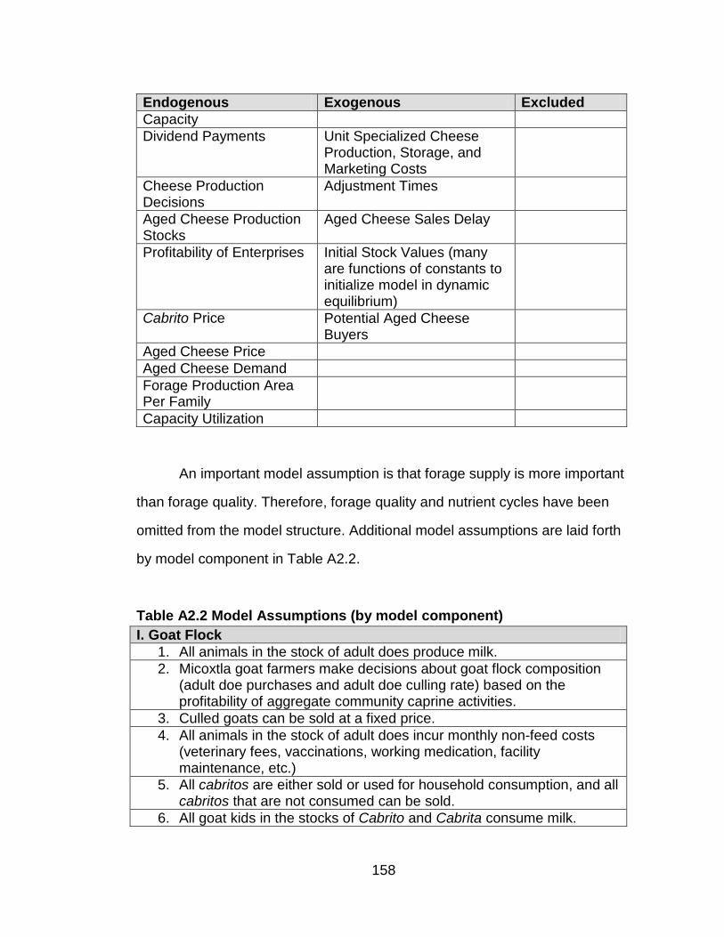
system dynamics models along with the imposed limits or model boundaries5
Of course, it is impossible to include all variables in the entire system.
Therefore, model boundaries must be specified based on the assessment’s
purpose (Thornton et al., 2003). Sterman (1991) noted, “For a model to be
useful, it must address a specific problem and must simplify rather than
.
In their general discussion of ex ante models, Antony and Anderson (1991)
explained, “The underlying biological processes either became irrelevant or
were oversimplified at high levels of aggregation” (p. 184). They suggested
that such high levels of aggregation are usually insufficient for project-level
analysis. However, the model evaluation and testing process includes tests of
boundary adequacy and structure assessment, which help to determine if the
amount of aggregation is appropriate for the model purpose.
5 In system dynamics modeling, boundaries are defined using an explicit boundary diagram comprising endogenous, exogenous, and excluded variables. System dynamics models often have wide boundaries that focus on endogenous factors, ignoring most detail complexity.
17
attempt to mirror in detail an entire system.” Thus, useful models are a
simplification of reality, addressing a specific problem within the broader
system framework. Depiction of a system rather than a problem with defined
boundaries would result in a model too complex to interpret, or to define its
assumptions.
van Ittersum et al. (2007) acknowledged the importance of developing
flexible generic models that encompass a greater variety of policy alternatives.
A generic model is more easily replicable and adaptable for similar ex ante
assessments. It could also be argued that quantitative simulation models are
inherently subjective, based on the experience, knowledge, and resulting
perceptions of the investigators. This criticism also applies to many classes of
models.
System dynamics modelers are typically more open to the inclusion of
“soft variables”. “Soft variables” are those with limited available data or those
that are difficult to measure or quantify (Sterman, 2000). Examples include
goals, human behavior, perceptions, expectations, desires, quality,
accumulation and flow of information, and parameters with limited data. This is
an advantage of the system dynamics methodology because these factors are
ignored by most modeling techniques and ex ante impact assessment
methods (Sterman, 1991). Ignoring these factors implies they do not influence
the system.
To identify and minimize sources of uncertainty and errors in depicting
real world processes, extensive sensitivity testing and evaluation are important
to an iterative model development process. System dynamics modelers
consider model validation to be infeasible because all models are
simplifications of reality. Validity can only be determined by its utility to model
18
users and stakeholders (Sterman, 2000). Intensive testing helps assure
usefulness. Twelve tests are established to evaluate structure, parameters,
behavior, errors, and sensitivity of the model. Numerical, behavioral, and
policy sensitivity tests can be conducted on a univariate or multivariate basis,
and are used to measure model response to changes in assumptions. The
ultimate robustness of a system dynamics model can be evaluated by
responses to changes in assumptions, and more importantly by the utility of
the model for end users.
2.1.4 Group Model Building
Group model building using system dynamics is widely used to increase
stakeholder participation and understanding of complex problems. It
encourages group learning, consensus building, and ownership of
interventions during the development process and with its results (Vennix,
1994; Vennix 1996). Thornton (2004) indicated that all stakeholders must be
“intimately involved” in the modeling process if the results are to be useful.
Extensive stakeholder involvement helps ensure model utility by meeting
stakeholder needs. Stakeholders include parties that are affected by or that
make decisions concerning the specified problem.
Participatory model building with interdisciplinary teams enhances the
final product with the distinct expertise, mental models, and opinions of the
participants (Spang, 2007). However, extensive participation in the model
development process can complicate the task. No standardized method has
been developed to conduct group model-building workshops, and it has been
identified as more of an art than a science, a problem leading to variable
results (Anderson et al., 1997). The success of group model building
19
workshops and courses often depends on the skill of the facilitator,
interactions among participants, and the degree of uncertainty in specifying
the problem.
Most group model building interventions are completed by an individual
or small group of consultants or expert modelers who work together with a
client stakeholder group to extract information about problem behavior
(Anderson et al., 2007; Beall and Ford, 2007; Luna-Reyes et al., 2006; Vennix,
1999; Anderson et al., 1997; Richardson and Anderson, 1995). These
strategic interventions are often solicited by clients on a contractual basis.
Behavior over time and pieces of stock-flow or feedback structure are
proposed and explained to attain consensus among the stakeholder group.
The process often begins with several small models called concept models
(Richardson, 2006). These easily understandable models are based on
preliminary research and information provided by the client. They are used to
facilitate initial understanding of system dynamics and to begin gathering more
precise information. The modelers later return to the client group with a
conceptual model or a simulation model that permits policy analysis for
stakeholder decision support.
During the modeling intervention process, the consultants facilitate the
information elicitation process using different scripts, participatory exercises to
extract information (e.g., problem description, key variables, reference mode
behavior, system structure, and parameter estimates from stakeholders) and
build model structure (Anderson and Richardson, 1997). An experienced
modeler works simultaneously to construct conceptual models and possibly
simulation models based on consensus information gathered from the
stakeholder group. This form of group model building can be quite effective but
20
does not normally build stakeholder capacity to learn systems thinking and
dynamic modeling techniques in order to construct models on their own.
Different from more typical group model building interventions, the
participatory group and team model building activities and exercises in this
study are part of intensive study of systems conceptualizations and system
dynamics modeling during the short course. The participants are also the
modelers in course exercises. Thus, the group model building activities are
designed to increase methodological comprehension while completing ex ante
assessments to increase understanding and build consensus about specific
problems. This “learning by doing” approach favors and compliments the
analytical and computational skill set of the course participants, and
importantly, their subject matter expertise about the selected problems.
The course involved participatory group and small team model building
exercises. For example, a preliminary model, which addresses a selected
agricultural development problem for organizational stakeholders, facilitates
system dynamics studies. Teams of three also completed initial steps of the
modeling process for other agricultural development-related problems during
the course. The author acted as a facilitator of development of the conceptual
model and simulation model.
2.1.5 Quantitative Versus Qualitative System Dynamics
Group exercises are used to develop conceptual models and simulation
models. Participants prefer a quick and direct path to problem solutions rather
than systematic completion of the modeling process (Stave, 2002). Similarly,
although participants may prefer a quantified simulation model at the
conclusion of the workshop, Vennix (1999) suggested that simulations need
21
not be the only objective. At times it is neither useful nor feasible to complete
the entire model-building process (Vennix, 1999). Thus, successful group
exercises have focused only on the qualitative model-development process
(Siemer and Otto, 2005). Quantification can either increase the understanding
of a problem or be misleading, resulting in questionable policy decisions
(Coyle, 1999).
In contrast, to obtain further insight about the problem through
simulation it is desirable to quantify a simulation model during a group model
building exercise. Furthermore, quantification can reveal behavioral responses
that are nearly impossible to infer from complex conceptual feedback structure
alone (Sterman, 2000).
The decision to quantify a model depends on a number of factors
including available time, facilitator expertise, participants’ background, group
size, group expertise, problem characteristics, and stage of preliminary model
development (Vennix, 1996). If system dynamics is determined to be
appropriate method for the selected problem, any one of these factors can be
the most limiting in the model-building process, and in deciding if quantification
is feasible.
2.1.6 System Dynamics Modeling/Research Process
The system dynamics modeling process is used to conduct the ex ante
problem analysis in this project paper. The iterative modeling process consists
of five phases (Sterman, 2000), which should be used to evaluate a problem
and analyze possible solutions. In this case, it is used as an ex ante problem
and policy analysis mechanism for INIFAP.
22
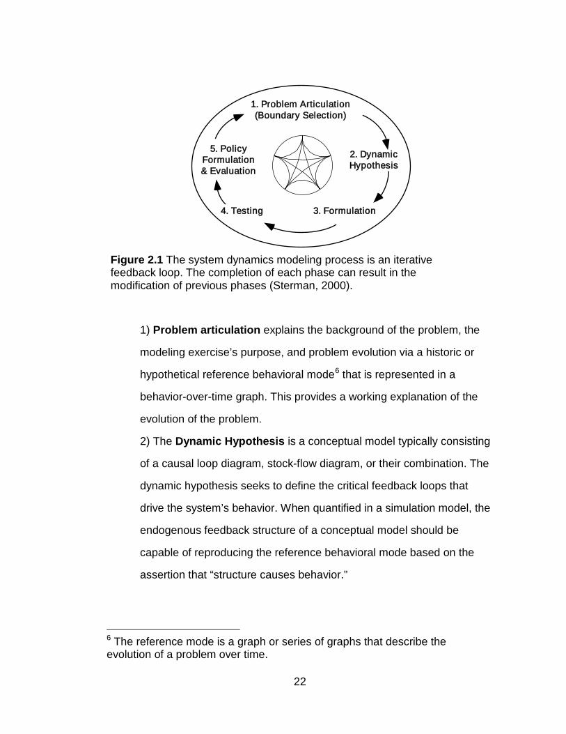
1) Problem articulation explains the background of the problem, the
modeling exercise’s purpose, and problem evolution via a historic or
hypothetical reference behavioral mode6
2) The Dynamic Hypothesis is a conceptual model typically consisting
of a causal loop diagram, stock-flow diagram, or their combination. The
dynamic hypothesis seeks to define the critical feedback loops that
drive the system’s behavior. When quantified in a simulation model, the
endogenous feedback structure of a conceptual model should be
capable of reproducing the reference behavioral mode based on the
assertion that “structure causes behavior.”
that is represented in a
behavior-over-time graph. This provides a working explanation of the
evolution of the problem.
6 The reference mode is a graph or series of graphs that describe the evolution of a problem over time.
1. Problem Articulation(Boundary Selection)
3. Formulation4. Testing
5. PolicyFormulation& Evaluation
2. DynamicHypothesis
Figure 2.1 The system dynamics modeling process is an iterative feedback loop. The completion of each phase can result in the modification of previous phases (Sterman, 2000).
23
3) The formulation of a simulation model is the transformation of the
conceptual model into explicit stock-flow structure. The model is
quantified (assigned parameter values and equations) so that
simulations can be conducted.
4) Model testing, or evaluation, consists of a series of tests to evaluate
the model’s robustness. Typically, comprehensive evaluation unveils
errors that cause one to return to previous phases in the iterative
modeling process. Sensitivity testing is also conducted here to evaluate
structure and variables with high uncertainty. Numerical, behavioral and
policy sensitivities to changes in parameters and structure are
evaluated relative to the model’s purpose.
5) Policy Formulation and Evaluation: Policy formulation and
evaluation often determines if the model is useful for the specified
purpose. In this phase, model users test policy options, interventions, or
actions to improve understanding about potential short-term and long-
term results, unintended consequences, and sources of policy
resistance. This should lead to improved decision making.
2.2 Professional Short Course on System Dynamics
The systems thinking and dynamic modeling course offered to INIFAP
Campo Experimental personnel was conducted from June to September 2007.
The course was developed in response to INIFAP’s desire to improve their
programs, promote multi-institutional and interdisciplinary collaboration, and to
add an ex ante dynamic conceptualization and simulation method to their
repertoire of technology and development mechanisms. The overall goal was
to build institutional capacity in ex ante impact assessment using system
24
dynamics methods and tools. The objectives for the short course were
designed to complement and enhance INIFAP goals.
2.2.1 Course Objectives
Participants will:
1) Learn the basics of systems thinking and dynamic modeling;
2) Increase knowledge about basic techniques for the ex ante assessment
of complex agricultural problems using system dynamics methods;
3) Complete group model building exercises to analyze and evaluate the
feasibility of dairy cooperatives to increase net economic returns in
highland communities, thereby building confidence in the value-added
cooperative model (Section 2.3);
4) Use system dynamics methods to model other problems for ex ante
decision support to improve project design, to identify information
needs, and to better serve INIFAP clients in mountain communities of
Veracruz.
2.2.2 Course Location
The course was held at INIFAP’s Campo Experimental offices in
Xalapa, Veracruz. The offices are located in the Secretaría de Agricultura,
Ganadería, Desarrollo Rural, Pesca y Alimentación (SAGARPA) facilities.
Three field trips to the rural community of Micoxtla supported team learning
and group model-building exercises.
25
2.2.3 Course Equipment, Supplies and Learning Materials
Equipment and supplies were provided by INIFAP. These included
laptop and desktop personal computers, an LCD projector, a white board, and
markers. Transportation for field trips was also provided by INIFAP. Vensim®
PLE software by Ventana Systems, Inc. was used to carry out modeling
exercises. Supporting literature (Appendix 1) and the course design were
assembled and developed by the author as described in Section 2.2.5.
2.2.4 Course Participants
There were eight consistent participants throughout the short course. A
total of sixteen participants attended at least one session. Seven of the eight
consistent participants were members of the multidisciplinary team stationed
at the Xalapa offices of INIFAP’s Campo Experimental. Among the seven
INIFAP participants, three were computer systems specialists that worked
primarily with GIS applications, statistical analysis, and various other software
applications. Three INIFAP participants were members of the micro-watershed
development team with specific training in agronomy, agricultural science, and
social science. The final INIFAP participant was an agronomist and the
director of the Campo Experimental at Teocelo. One additional participant
was a student in the School of Economics at the University of Veracruz in
Xalapa.
2.2.5 Course Structure
The short course was structured based on the Applied Economics and
Management (AEM) 494 “Introduction to System Dynamics Modeling” and
AEM 700 “System Dynamics Applications” courses taught by Dr. Charles
26
Nicholson at Cornell University. A previous short course titled “Application of
System Dynamics to Agricultural Settings in the Gulf Region of Mexico” was
also used as a general guideline for lectures, materials, and exercises
(http://tiesmexico.cals.cornell.edu/courses/shortcourse5/). The previous short
course was taught by Dr. Charles Nicholson in 2005 at the Universidad
Veracruzana in Veracruz Port.
The course consisted of three components: introductory system
dynamics coursework, group model building exercises related to value
addition to goat’s milk, and small team model-building exercises for selected
problems. The three components were complementary, providing both
theoretical and practical learning opportunities for course participants. First,
theoretical course materials were presented weekly in two or three two-hour
sessions. Practical exercises complemented the theoretical lectures. The
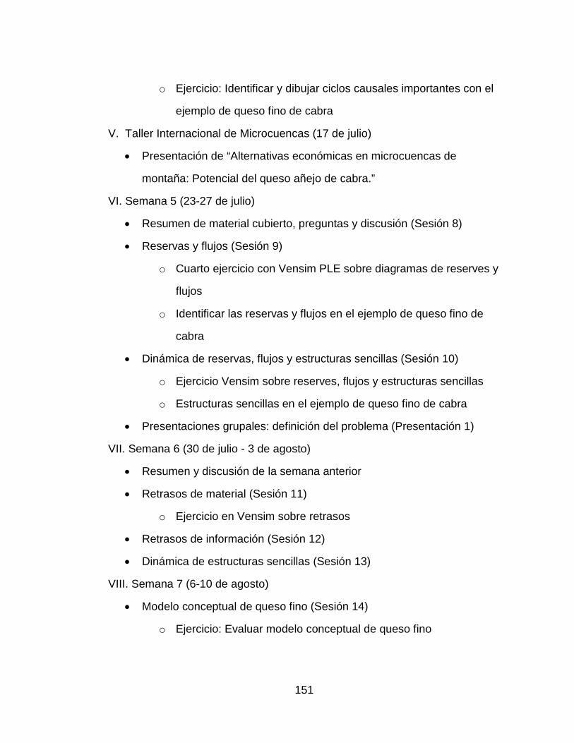
course session outline in Appendix 1 includes the final two-day workshop and
supporting literature. The final workshop was designed to review materials
covered during the course, to address additional topics in response to
participant feedback, and to define future strategies for potential system
dynamics applications by the INIFAP team.
Second, a case study of the economic feasibility of value addition to
goat’s milk and the marketing of cheese made from it by a hypothetical rural
dairy cooperative was a core component of the course. The ex ante
assessment was designed to determine if aged goat cheese could be a
feasible economic alternative for farmers in Micoxtla. This group model-
building component was completed using a preliminary version of a system
dynamics model developed by the author (Section 2.3). The objectives of
INIFAP participation in the model building process were to facilitate group
27
learning, to evaluate the preliminary model, and to generate confidence in
future model specifications. Course participants first examined and evaluated
the preliminary simulation model as a participatory learning mechanism. The
expert subject matter knowledge and direct observations provided by INIFAP
researchers and technicians helped to improve the accuracy of the case study
and of the model. This participation also assured that the simulation model
could be a useful resource for learning system dynamics, and a useful policy
analysis mechanism for the ex ante evaluation of cheese cooperative
management.
The case study, described in Section 2.3, was completed using the
system dynamics modeling process (Section 2.1.5). Importantly, it illustrated
problem conceptualization and simulation model formulation as an ex ante
impact assessment mechanism for agriculture and rural development.
Third, small teams initiated their own analytical modeling processes
focusing on specific problems related to their research interests and own
experiences. Course participants were divided into three teams of similar
interests, experiences, and roles in INIFAP. Teams were instructed to select
an appropriate dynamic problem of interest to the INIFAP Campo
Experimental. After problem selection, the teams completed the initial steps of
the system dynamics modeling process. They focused primarily on the initial
qualitative phases of the modeling process, also developing incipient
simulation models. Each team presented its model development progress on
three occasions during the course. These presentations provided an
opportunity for detailed discussion by multi-disciplinary INIFAP faculty. The
first presentation described the selected problems. The second presentation
conceptualized the problem and represented the dynamic hypothesis for the
28
modeling process. The third presentation explained the results of an initial
attempt to formulate a simulation model. Each of the three presentations was
cumulative, but required revision of the previous phases based on facilitator,
participant, and non-participant feedback both during and after the
presentations. This informal INIFAP supervisor and peer review process
enriched group thinking and improved future iterations in the modeling process
for all teams. Therefore, team model development was an iterative learning
process benefitting all course participants.
2.3 Value-Added Cooperative Model
The value-added cooperative model was designed with INIFAP as an
adaptable policy analysis tool for the assessment of value-addition to
agricultural products. The dynamic biophysical and socioeconomic model
represents the aggregate caprine resources in Micoxtla and a rural value
addition and marketing cooperative. The model consists of nine components:
cooperative management and decisions, 7) aged cheese market, 8) producer
profitability expectations, and 9) user interface. The ensuing description
summarizes the background, problem conceptualization, and structure of the
simulation model.
2.3.0.1 Model History
An ex ante assessment of the economic feasibility of goat cheese
production in the Veracruz highlands was initiated in 2007 in the introductory
system dynamics course at Cornell University. The resulting problem analysis
29
and preliminary simulation model were used to illustrate and teach the short
course (Section 2.2) to INIFAP researchers and extension workers. The
preliminary model was employed in group model building exercises to improve
understanding of the modeling process. Course participants also contributed
expert viewpoints for model improvement during sensitivity testing and model
evaluation exercises. Finally, participants conducted some policy analysis
using the model’s user interface.
2.3.0.2 Micoxtla Community Background
Micoxtla is a small highland community located in the municipality of
Xico, Veracruz, Mexico at an altitude of 2,040 meters on the eastern slopes of
Cofre de Perote mountain in the Sierra Madre Oriental mountain range. The
approximate geographic coordinates are 19° 27' N and 97° 2' W. The
population of this rural community is about 260 people. The community is
situated in the Coatepec micro-watershed, one of three action areas for
INIFAP’s micro-watershed development programs.
Agricultural production consists of two staple crops, maize and beans,
as well as potatoes, forages, and patio vegetable production (INIFAP, 2006b).
Most households also raise goats and chickens. Only a few families raise
hogs, cattle, and sheep. The majority of agricultural land lies on steep slopes
where soil erosion is a chronic problem. Families cultivate an average of 2.3
hectares. Four-hundred and sixty-six hectares of private and communal
agricultural, pasture, and forest land delimit Micoxtla. Most agricultural
activities are for household consumption. INIFAP has been collaborating with
the community since 2003 on various community and agricultural development
30
activities. Their work is now undergoing a transition into micro-watershed
investigation and water conservation.
According to Díaz Padilla (personal communication, July 5, 2007), a
Micoxtla family must earn an average of $5,500 pesos per month (U.S. $550
at an exchange rate of $10 pesos per dollar) to comfortably sustain their
livelihoods. If families do not reach this income benchmark, the presumed
likelihood of emigration from the rural community is greatly increased. One of
INIFAP’s primary objectives is to help Micoxtla families surpass this
benchmark.
2.3.0.3 Micoxtla Economic Activities
The majority of Micoxtla’s inhabitants work primarily in agricultural
production, although some individuals travel to the surrounding cities of Xico,
Coatepec, and Xalapa where employment opportunities are more plentiful. In
addition, many community members seasonally migrate to nearby coffee
plantations in the Teocelo region to harvest coffee. INIFAP (2006b) found that
most Micoxtla families struggle with seasonal food insecurity and economic
instability. The principal products sold are milk, young goats for meat (cabrito),
and eggs after fulfilling household consumption needs (INIFAP, 2006b).
Nearby Xico (five kilometers), a tourist destination, provides a ready market
outlet. Larger population centers and markets are also located in Coatepec (12
km) and Xalapa (25 km).
An array of traditional products is produced in Micoxtla and could allow
community members to compete in higher-value local and regional markets.
According to Ramírez-Farías (2001), one effective way to compete in these
31
markets is to produce differentiated products based on consumer demand and
product acceptance.
2.3.1 Problem Description
An important source of income for Micoxtla families is the sales of
caprine products: milk and meat (cabrito). However, production is low and net
income is modest. Currently, most milk is sold directly to a local milk
processing plant at 3.5 to 4.5 pesos7
Micoxtla community members identified the low earnings from goat’s
milk as a processing and marketing problem stating, “We don’t know how to
prepare higher quality cheeses and don’t have a place to sell them” (INIFAP,
2006b). Micoxtla farmers have expressed an interest in learning to produce
and sell new types of cheese with the objective of increasing profits from
goat’s milk and improving household economic conditions. Consequently,
among the numerous options to generate additional income in Micoxtla, this
strategy was chosen for this collaboration. Therefore, ex ante assessment of
the feasibility of value-added goat’s milk production, processing, and
per kg, varying seasonally (INIFAP,
2006b). Micoxtla family members walk up to ten kilometers per day to sell as
little as one kg of milk, which indicates the importance of this cash income.
Aged, or premium, cheese production in Micoxtla could provide an opportunity
to increase household earnings from dairy products, an idea originating in the
community itself. Milk that is not sold is either consumed in the household or
used to produce traditional fresh cheese. Similar to raw milk, this cheese
product adds little value and its profitability is low.
7 The exchange rate in 2008 was approximately ten Mexican pesos per one U.S. dollar.
32
marketing by the hypothetical dairy cooperative was undertaken as a project
study and as a mechanism for the application of system dynamics principles in
response to community initiative. In addition to milk, cabrito production and
sales were also considered.
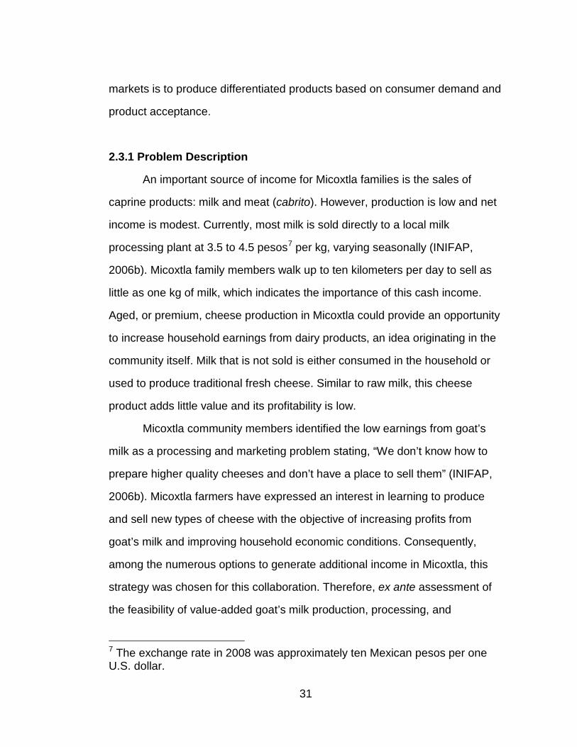
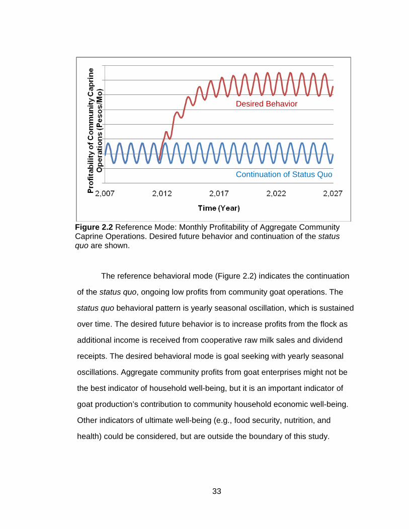
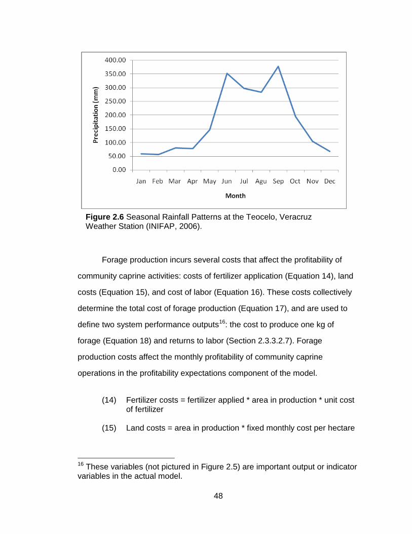
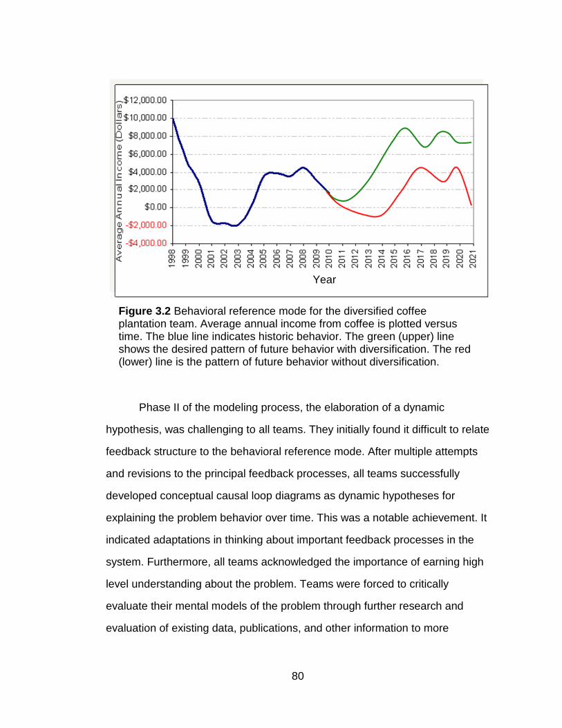
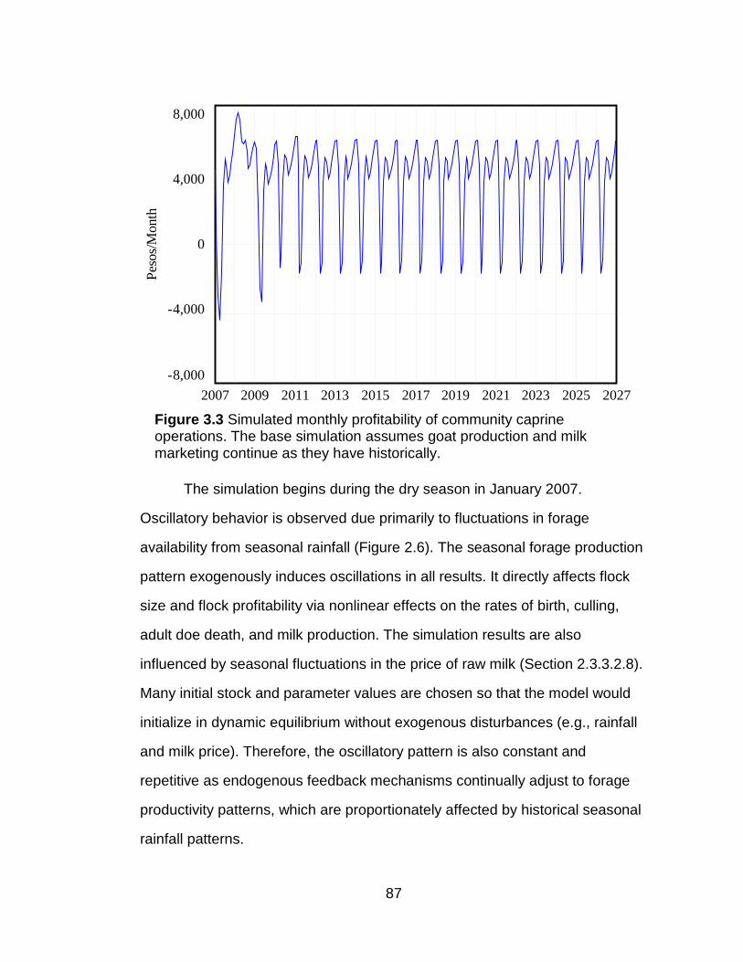
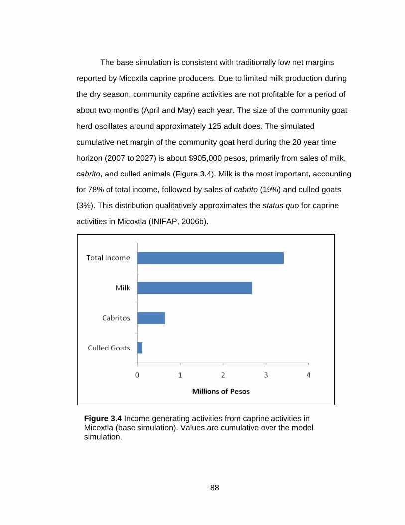
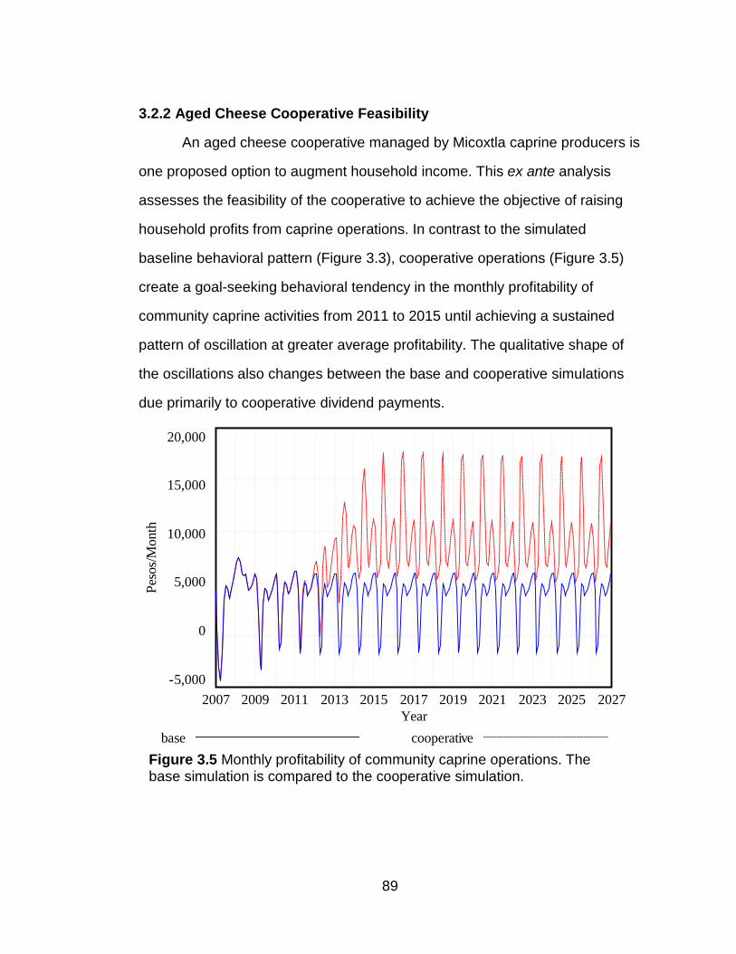
2.3.1.1 Reference Mode
The reference mode graph (Figure 2.2) illustrating monthly profitability
from aggregate community goat operations includes income from culled
animals, cabrito, fluid milk sales in Xico, fluid milk sold to the cheese
cooperative, and dividends paid by the cooperative. To compute profits,
animal production costs, forage production costs, and milk production and
marketing costs are subtracted from income.
Although historical data are unavailable, producer perceptions suggest
that profits from goat enterprises are low and uniform in the region. Seasonal
fluctuations in profit are influenced by seasonal rainfall and forage supply and
milk price instability. By adapting milk processing to include higher-value aged
cheese, profits could increase. The target market is the growing tourism
industry in the region, especially in the nearby town of Xico. A time horizon8
of
20 years was chosen to assess future patterns of behavior after initiating aged
cheese cooperative operations. The 20-year time horizon is sufficient to
capture major changes (e.g., collapse) in profits from limiting factors such as
forage and market instability.
8 The time horizon is the past and future time necessary to describe the historic and hypothesized behavior of the problem.
33
The reference behavioral mode (Figure 2.2) indicates the continuation
of the status quo, ongoing low profits from community goat operations. The
status quo behavioral pattern is yearly seasonal oscillation, which is sustained
over time. The desired future behavior is to increase profits from the flock as
additional income is received from cooperative raw milk sales and dividend
receipts. The desired behavioral mode is goal seeking with yearly seasonal
oscillations. Aggregate community profits from goat enterprises might not be
the best indicator of household well-being, but it is an important indicator of
goat production’s contribution to community household economic well-being.
Other indicators of ultimate well-being (e.g., food security, nutrition, and
health) could be considered, but are outside the boundary of this study.
Desired Behavior
Continuation of Status Quo
Figure 2.2 Reference Mode: Monthly Profitability of Aggregate Community Caprine Operations. Desired future behavior and continuation of the status quo are shown.
34
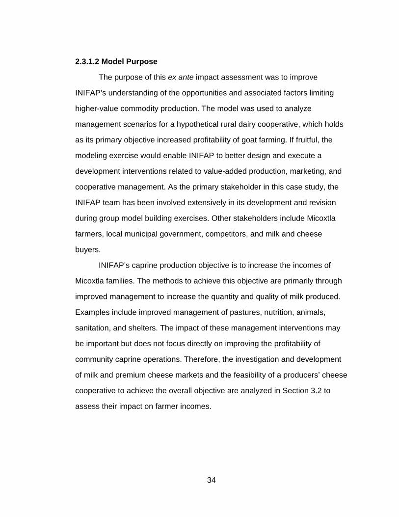
2.3.1.2 Model Purpose
The purpose of this ex ante impact assessment was to improve
INIFAP’s understanding of the opportunities and associated factors limiting
higher-value commodity production. The model was used to analyze
management scenarios for a hypothetical rural dairy cooperative, which holds
as its primary objective increased profitability of goat farming. If fruitful, the
modeling exercise would enable INIFAP to better design and execute a
development interventions related to value-added production, marketing, and
cooperative management. As the primary stakeholder in this case study, the
INIFAP team has been involved extensively in its development and revision
during group model building exercises. Other stakeholders include Micoxtla
farmers, local municipal government, competitors, and milk and cheese
buyers.
INIFAP’s caprine production objective is to increase the incomes of
Micoxtla families. The methods to achieve this objective are primarily through
improved management to increase the quantity and quality of milk produced.
Examples include improved management of pastures, nutrition, animals,
sanitation, and shelters. The impact of these management interventions may
be important but does not focus directly on improving the profitability of
community caprine operations. Therefore, the investigation and development
of milk and premium cheese markets and the feasibility of a producers’ cheese
cooperative to achieve the overall objective are analyzed in Section 3.2 to
assess their impact on farmer incomes.
35
2.3.2 Model Conceptualization
The development of a conceptual model using system dynamics
methods typically employs causal loop diagrams and stock-flow diagrams. A
causal loop diagram consists of a set of feedbacks that collectively define the
structure of the system, which is hypothesized to generate its behavior
(Sterman, 2000). The conceptual diagram is a structural hypothesis to explain
the behavioral reference mode. There are two classes of feedback loops.
Positive or reinforcing loops typically stimulate growth whereas negative or
balancing loops slow growth, producing oscillation when delays9
are present.
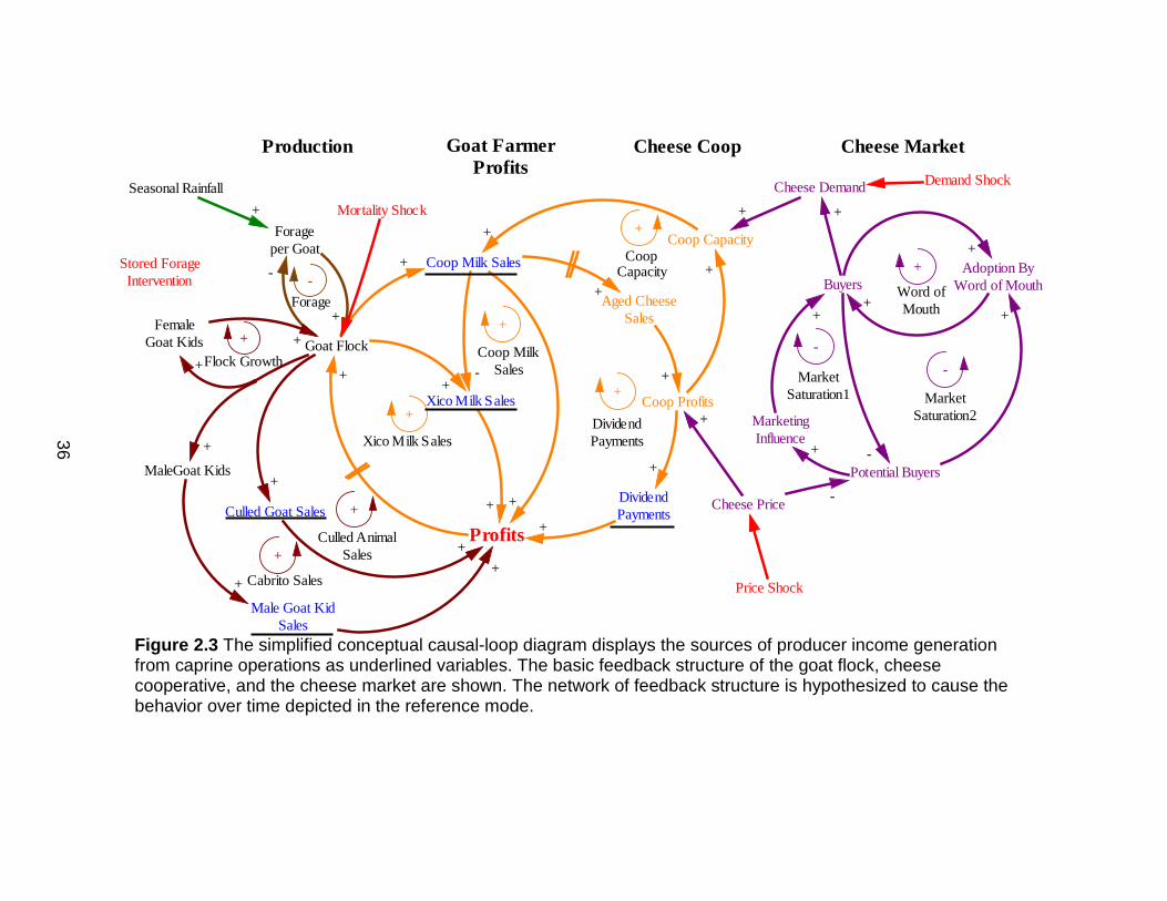
2.3.2.1 Model Feedback Structure
There are several key feedback pathways for the five income
generation activities associated with goat production in Micoxtla (Figure 2.3).
These activities include milk sales in Xico, cooperative milk sales, cooperative
dividend payments, sales of culled animals, and male kid (cabrito) sales. Each
activity creates a positive or reinforcing feedback loop leading to system
growth in the absence of limitations. The only negative or balancing feedback
loop in the production side is forage supply. Additional balancing feedback
processes are found on the market side. More detailed feedbacks have been
omitted for simplicity.
9 In causal loop diagrams, a delay process is represented by two perpendicular lines in a causal link.
36
Figure 2.3 The simplified conceptual causal-loop diagram displays the sources of producer income generation from caprine operations as underlined variables. The basic feedback structure of the goat flock, cheese cooperative, and the cheese market are shown. The network of feedback structure is hypothesized to cause the behavior over time depicted in the reference mode.
Goat FarmerProfits
Xico Milk Sales
Production
Goat Flock
Forageper Goat
Cheese Coop
Coop Milk Sales
Aged CheeseSales
+
DividendPayments
Profits
+
+
-
+
+
+
+
+
+
Coop Capacity
Cheese Demand+
+
Seasonal Rainfall+
+
+
+
+
-
Coop Profits
+
+
Cheese Price
+
Mortality Shock
Price Shock
Demand Shock
Stored ForageIntervention
Xico Milk Sales
Forage
Coop MilkSales
DividendPayments
CoopCapacity
BuyersAdoption By
Word of Mouth
Potential Buyers-
+
+
+
MarketingInfluence
+
+
-
+Word ofMouth
+
--Market
Saturation1 MarketSaturation2
Cheese Market
MaleGoat Kids
Culled Goat Sales
-
Male Goat KidSales
+
++
+
+
Cabrito Sales
+
Culled AnimalSales
FemaleGoat Kids
+
+
++Flock Growth
37
The historic and undesired pattern of future behavior in the behavioral
reference mode (Figure 2.2) is explained by dynamic equilibrium10 in all stocks
except those in the cheese cooperative and cheese market components of the
model, which are inactive and in static equilibrium11
The market, although it is exogenous to the rest of the model in the
conceptual diagram, contains additional balancing feedback loops that limit
system growth. Goal seeking or capacity seeking behavior is driven by
multiple feedbacks. Constraints that contribute to goal seeking behavior in the
profitability of goat operations include milk production capacity, cheese
production capacity, seasonal forage production costs, dividend payments,
sales of cabrito and culled animals, and overall flock profitability. Farmer
perceptions, desires, and cost limitations have been omitted, but they also
collectively play a role in defining the goal seeking capacity limit. Nonlinear
dynamics permit feedback loop and capacity dominance to shift during a
(Figure 2.3) is activated by initial marketing of value-added product, which
then initializes cheese cooperative operations. This includes the cooperative
milk sales, dividend payments, and capacity feedback loops.
Specifically, increases in the profitability of community caprine
operations are inferred from the dividend payments feedback loop. Market size
and cheese production capacity generate the initial capacity constraint. After
the initial market expansion occurs and cheese production capacity
10 Dynamic equilibrium occurs when the inflows to each stock are equal to the outflows. Consequently, the stock values do not change over time. 11 A stock is in static equilibrium when all inflows and outflows are inactive or equal to zero.
38
investments are fulfilled, milk supply and market capacities shift seasonally,
thus determining the capacity for value-added product production and sales.
2.3.3 Simulation Model Description
The simulation model represents the community caprine resources in
Micoxtla. Twenty-five families own approximately 300 goats (INIFAP, 2006b).
Flock management is carried out at the household level. Families allow their
individual flocks to graze several hours per day on Micoxtla’s communal
pasture and forest lands. Families also cut and carry forages, such as forage
oats and rye grass, to feed animals when they are enclosed in corrals and
sheds. Some families seasonally supplement with cracked maize and minerals
to support animal health.
Despite apparent complexity, most biophysical relationships and
decision rules are straightforward and aggregated. Consequently, the
adaptable model depicts the primary interactions and constraints to the
economic success of value-added cheese production for a rural cooperative.
2.3.3.1 Reference Mode Accounting
Three caprine enterprises are considered in the reference mode. First,
in the flock enterprise, culled does are sold at a nominal price ($300
pesos/doe). In addition, young bucks (cabritos) are sold in Xico to make a
traditional Mexican dish ($300 pesos/cabrito). The flock enterprise is charged
for non-feed animal costs at a constant monthly rate ($5 pesos / (goat *
month)). The second enterprise is fluid milk production and sales. Milk can
either be sold in Xico (Equation 16) or to the cooperative (Equation 15). This
farm level enterprise is charged a fee of two pesos per kg for milk marketing
39
and transport. The community caprine operation can also receive income from
the cheese cooperative as dividend payments (Section 2.3.3.2.7). The entire
goat operation is charged for forage production costs (Section 2.3.3.2.2). The
behavioral reference mode, monthly profitability of community caprine
operations, represents the profitability of the community flock, rather than the
outcomes for an individual farm household (Figure 2.2). When the community
enterprise is profitable, farmers reinvest in the flock by purchasing adult does
(Section 2.3.3.2.1).
The third enterprise, the aged cheese cooperative (Sections 2.3.3.2.4 to
2.3.3.2.7), is independent of animal production and milk sales. The
cooperative buys fluid milk from farmers and incurs expenses for cheese
production, storage, and marketing. The cooperative’s profits are invested in
productive capacity or redistributed to participating farmers as dividend
payments.
2.3.3.2 Model Components
The simulation model consists of nine components: the aggregate
community goat flock, forage resources, milk allocations, cooperative aged
cooperative cash flow and decisions, farmer profitability expectations, and an
interactive user interface. When seasonal rainfall patterns and seasonal milk
price oscillations are not exogenously imposed, the model initializes in
dynamic equilibrium. Dynamic equilibrium is achieved because the inflows and
outflows from each stock are equal and stocks are unchanged. All nonlinear
40
table functions12
are normalized to assure dynamic equilibrium except for the
aged cheese cooperative and market components, which initialize in static
equilibrium because the cooperative is not processing milk at the outset. In
addition, some initial values for stocks and parameters are selected for
dynamic equilibrium. A description of the assumptions, boundary, and
parameters of the model is included in Appendix 2. The simulation model was
formulated in Spanish to facilitate use by the INIFAP team.
2.3.3.2.1 Community Goat Flock
12 Table functions, also called lookup functions, normally use a proportion of a variable to its reference value to compute its effect on another variable. To initialize a model in dynamic equilibrium, the proportion is equal to one, which does not affect the default or reference value for the affected variable.
Figure 2.4 Simplified Goat Flock Stock-Flow Structure. The community goat flock structure is organized into four stocks to represent flock management. Cabritos and cabritas are young male and female goats, respectively.
41
The stock-flow structure of the goat production component of the model
consists of a doe aging chain divided into three stocks: cabritas (young does),
weaned cabritas, and adult does. An additional stock of cabritos (young bucks)
is also part of the goat production stock-flow structure but is not included in the
aging chain because all young male goats are either sold or consumed locally.
These four stocks constitute the goat flock. The fractional kidding rate
(Equation 1) is a function of the birthing interval, the number of kids per
parturition, and the number of adult does. This fractional rate varies based on
the fulfillment of required forage needs through a reference multiplicative
formulation13
. The fractional kidding rate is uniformly distributed so that 50
percent of the kids are males and 50 percent are females.
effect of forage availability on fractional kidding rate(fraction of forage needs met)
This simple kidding formulation could be compared to or revised based
on the more complex productivity index proposed by Bosman et al. (1997).
The Bosman index measures performance at the individual animal-level. It
also considers the age at first parturition, the age at subsequent parturitions,
and the live weight of the litter at weaning. Therefore, doe productivity is
measured in live weight per year rather than as a simple fractional kidding
rate.
13 The reference multiplicative effect is a common system dynamics formulation that multiplies a variable’s reference value by a nonlinear effect that is dependent on an additional variable or variables. The nonlinear effect is often normalized to return the reference value under initial, known, or default conditions. The effect uses a lookup function.
42
The cabrita stock is affected by one inflow, the cabrita kidding rate, and
two outflows, the death and weaning rates. The weaning rate, an intermediate
flow between the cabritas and weaned cabritas stocks, is a third-order delay of
the cabrita kidding rate and depends on the constant average weaning age.
The weaned cabritas stock has only one outflow, a high-order (eighth) delay in
the weaning rate. The combined weaning and maturation delays form a
higher-order delay distribution around the total average delay time for doe
maturation. Cabritas must reach their first parturition (kidding) to complete
maturation to adulthood, which is represented by entry into the stock of adult
does. The age at first parturition is slightly over two years (G. P. Alvarez
Montes de Oca, personal communication, August 16, 2007). It is assumed that
all adult does produce milk.
The stock of adult does has an additional inflow, purchased animals,
and two first-order outflows, the rates of culling and mortality. It is assumed
that Micoxtla producers make decisions about flock composition based on the
profitability of the enterprise. The culling rate (Equation 4) changes with
average time in the flock, a variable that changes as a function of the ratio of
desired adult does to actual does (through a reference multiplicative
formulation). When the desired number of adult does exceeds the actual
number of adults, does are purchased (Equation 5) and the culling rate
decreases (Equations 3 and 4). The desired adult does variable (Equation 2)
is defined by a reference multiplicative formulation that adjusts based on the
actual number of adult does and expected profitability of the goat operation.
Does can be purchased when sufficient cash is available and the desired
number exceeds the actual count of adults. The desired does and doe
43
purchase formulations were adapted from the production capacity formulation
in Sterman (2000).
(2) Desired does = adult does * effect of profitability on desired does (ZIDZ((expected profitability-reference profitability), reference profitability))14
(3) Average time in flock = MAX (base average time in flock * effect of ratio of desired adult does to adult does on average time in flock (ZIDZ(desired adult does, adult does)), minimum time in flock)15
(4) Culling rate = adult does/average time in flock
(5) Doe purchase rate = MAX ((MIN (purchases permitted based on available cash, (desired adult does – adult does) / desired adult does adjustment time)), 0)
The adult doe mortality rate is determined by the fractional mortality
rate. This is a function of several parameters so that the model initializes in
dynamic equilibrium. The fractional rate is also allowed to vary according to
forage availability via a reference multiplicative formulation.
It is assumed that all culls can be sold at a fixed price and that all
animals in the stock of adults incur monthly non-feed costs. Therefore, sales of
culled animals and monthly non-feed costs affect the monthly profitability of
the aggregated community caprine operation.
The cabritos stock is affected by the fractional kidding rate inflow and
goat sales and consumption outflow. The outflow is a third order delay of the
inflow. It is assumed that all cabritos are either sold or used for household
14 ZIDZ means “zero if divided by zero.” When that the denominator is equal to zero, the function returns a value of zero instead of producing a floating point error due to division by zero (Ventana Systems, Inc., 2008). (e.g., ZIDZ(10,0) = 0) 15 The MAX function returns the higher of two possible values (Ventana Systems, Inc. 2008). (e.g., MAX (4,7) = 7)
44
consumption, and all that are not consumed are sold. Cabrito sales revenues
are determined by the number of animals sold and a constant cabrito price. All
kids in the stocks of cabritos and cabritas consume milk.
Adult males are not modeled explicitly because most Micoxtla
producers do not maintain breeding bucks. The few producers that do own
breeding bucks lend them to other producers, which sometimes incurs small
breeding fees that were ignored and excluded from the model boundary
(INIFAP, 2006b).
2.3.3.2.2 Forage Resources
The animal aging chain is connected to the forage resources
component through the forage available per caput (Equation 6) and fractional
Figure 2.5 Simplified forage stock-flow structure. Multiple balancing feedback loops regulate forage production and consumption based on forage availability. Rainfall directly affects forage productivity.
45
forage needs satisfied (Equation 7). The ratio of available forage to reference
forage per goat defines the fraction of forage needs that are met (Equations 6
and 7). This fractional forage condition nonlinearly affects the kidding rate,
adult goat mortality, milk production, and desired forage resources via their
respective reference multiplicative effect formulations in other model
components. This forage resources formulation does not account for forage
quality. Bosman et al. (1997) proposed equations that could be adapted to
represent forage quality and animal maintenance requirements. They
simulated animal productivity in response to changes in several parameters
such as feed intake, feed quality, and flock composition. More complex
equations used in their analysis were not implemented here to maintain a
more simplified model that aims to capture only the key effects of flock
management and value addition to agricultural production. Thus, forage quality
was excluded from the current model boundary. As a result, the key
assumption in the forage resources component of the model is that at this
incipient stage of production the quantity of forage produced on a limited
amount of land is relatively more limiting on the caprine enterprise than its
quality.
(6) Forage available per caput = ZIDZ(forage resources, adult goats +
weaned cabritas)
(7) Fractional forage needs satisfied = forage available per goat / reference forage required per goat
The forage resources component of the model consists of one stock
(forage resources) with its production inflow and consumption outflow. If
farmers perceive their forage resources to be insufficient, it is assumed that
46
they will desire to increase forage production through productivity increases
and land area expansion. Both land productivity and land in production are
anchored on their reference values in reference multiplicative formulations.
Indicated land area changes via a reference multiplicative formulation so that
more land is desired when forage resources are perceived to be inadequate
(Equation 8). Furthermore, producers also slightly increase fertilizer
applications (Equation 9) when forage productivity is inadequate to meet flock
needs. INIFAP worked with Micoxtla farmers to improve crop productivity by
applying fertilizer. The inclusion of this policy in the model assumes that
producers recognize the potential for increased returns with productivity gains
from fertilizer applications, and that they have the capacity to purchase
fertilizer or apply manure. A first order delay formulation with a three-month
delay time is used in the indicated forage productivity variable (Equation 10) to
calculate productivity changes from fertilizer application.
(8) Indicated land area = base amount of land in production per family *
effect of perceived required forage needs met on desired area (smooth fractional forage needs satisfied)
(9) Fertilizer applied = reference fertilizer application * effect of perceived required forage needs met on fertilizer application(smooth fractional forage needs satisfied)
(10) Indicated forage productivity = SMOOTH (base forage productivity * effect of fertilizer on productivity(fertilizer applied / reference fertilizer application), fertilizer effect on forage productivity adjustment time)
Forage productivity (Equation 11) is either equal to indicated forage
productivity or seasonal forage productivity (Equation 12). Seasonal land
47
productivity changes with the pattern of rainfall though the effect of seasonal
forage consumption per goat * (effect of forage availability on consumption (ZIDZ(forage available per goat, reference forage available per goat)))
50
2.3.3.2.3 Milk Allocations
The milk allocations component of the model represents the use
distribution of fluid milk for feeding kids, for household consumption, and for
sales income. It is linked to the goat production component of the model
through the stocks of adult does, cabritos and cabritas, and to the forage
resources component through forage availability (forage supply). Reference
multiplicative formulations were used to represent the nonlinear relationships
in variables for the amount of milk consumed by the household consumption
and the daily milk yield per nanny. The amount of milk for household
consumption decreases when profitability from milk sales and cheese
production surpasses the reference value. Milk for goat kid consumption varies
as the number of young goats varies. Producers indicated that they do not
restrict the amount of milk consumed by kids. Therefore, a constant daily
amount was assumed (G. P. Alvarez Montes de Oca, personal
Figure 2.7 A simplified structure of milk allocations. Fluid milk is consumed by goat kids and the families raising them. Leftover milk production is allocated to income generation, and is either sold in Xico or to the aged cheese cooperative.
Milk Production
Milk Consumed byGoat Kids
Milk Consumed byFamilies
Milk for IncomeGeneration
Milk Sold in Xico
Milk Sold to AgedCheese Enterprise
Desired Milk Sales
+
+
-
+
+
--
+ -
+
Adult Does
+
Forage Availability
+
ExpectedProfitability of Milk
-
51
communication, August 16, 2007). Milk production also varies based on forage
availability, animal intake, and lactation period.
Any leftover milk after consumption by kids and the household is sold
(Equation 20). The model begins with all milk available for income generation
activities being sold in Xico. In order for milk to be allocated to produce aged
cheese, an initial investment to establish productive capacity is required. This
initial investment was assumed to occur at the simulation start time (January
2009). The assumption was made that producers will first fill the demand of
the cheese cooperative before selling excess milk in Xico (Equations 21 and
22).
(20) Milk for income generation = MAX((milk production-milk
consumed by kids-milk consumed by families) , 0)
(21) Milk sold to aged cheese enterprise = MIN(milk production for income generation, desired milk sales)
(22) Milk sold in Xico = milk production for income generation – milk
sold to aged cheese enterprise
52
2.3.3.2.4 Premium Aged Cheese Production
Once production capacity is established (Section 2.3.3.2.6), purchased
milk enters the aged cheese component of the model. Cheese production is
determined by its yield from the processing of fluid milk (Equation 23). This
production rate is an inflow to the aging cheese stock. The maturation rate
(Equation 24) is the intermediate flow between the aging cheese stock and the
inventory stock. It is a fixed delay of the cheese production flow. After
maturation, the product is transferred to the aged cheese inventory stock. It
exits this stock through the order fulfillment rate (Equation 25), which is a
variation of the Fuzzy MIN function suggested by Sterman (2000). Orders are
Figure 2.8 Simplified stock-flow structure of cooperative aged cheese production consisting of a two-stock aging chain.
53
filled based on consumer demand and available inventory. Order fulfillment
means cheese sales to consumers and is the sole source of income for the
cooperative.
Variables depicting production costs, storage costs, and marketing
costs are determined by the quantity of cheese being produced, stored, and
sold, respectively. The unit cheese production costs (Equation 26) decrease
over time as members of the cooperative acquire cheese making experience.
Another major cost for the cooperative is the raw milk input, which the
cooperative buys from producers.
(23) Production rate = cheese yield * milk sold to aged cheese
(25) Order fulfillment rate = desired order fulfillment rate * order
fulfillment table(ZIDZ(maximum order fulfillment rate, desired order fulfillment rate))
(26) Unit costs = base unit costs *(cumulative experience / initial
experience) ^ strength of learning curve
The aged cheese price affects cheese revenues. The difference
between revenues and costs is defined as the monthly profitability of aged
cheese production. It also affects the cumulative aged cheese profitability
stock and the exponentially smoothed monthly profitability of aged cheese in
the profitability expectations component of the model.
54
2.3.3.2.5 Aged Cheese Market
The hypothetical aged cheese market is a niche market in Xico. Clients
in this hypothetical market are hotels and restaurants that serve the growing
tourism industry. The aged cheese market demand structure is also the source
of the expected S-shaped pattern of growth in the number of actual buyers
(e.g., restaurants, hotels, and private households). This directly affects the
product demand, the desired cooperative production capacity, and capacity
utilization. The expected S-shaped growth is generated by this structure in the
cooperative simulation (Figure 2.10). The structure was selected and adapted
from the Bass Diffusion Model (Bass, 1969, as cited in Sterman, 2000), which
is commonly used to estimate new product sales during the product growth
Figure 2.9 Simplified aged cheese market growth structure. The typical two-stock market growth structure (Sterman, 2000) was adapted to interface with unit costs and the price of aged cheese.
55
phase. It normally simulates an S-shaped growth pattern in the number of
product adopters, and, in this case, in the aggregate demand for premium
cheese.
The population of potential buyers (Equation 27) is determined by the
population of total buyers, the current number of actual buyers, and the
fraction of the population willing to adopt the product. The number of potential
buyers is constrained by the fraction of the total population willing to adopt,
which prevents the entire population from becoming potential buyers unless
the price of aged cheese is extremely low. The adoption rate (Equation 28) is
the only inflow into the actual buyers stock. It is the sum of adoption from
interaction and adoption from word of mouth. Adoption from word of mouth
(Equation 29) depends on the interaction between actual buyers and potential
The general productive capacity structure was adapted from
Henderson’s (2007) early growth stage cooperative modeling work. The aged
cheese cooperative initializes its operations by making a small initial
investment in production capacity at the same time that marketing
commences, which is year two of the simulation (January 2009) given default
assumptions. Following an exogenous initial investment, the capacity
expansion structure acquires capacity endogenously. The capacity expansion
inflow (Equation 30) to the capacity stock permits expansion when there is a
desired capacity investment (Equation 31) and financial conditions in the
cheese cooperative allow for capacity investment. The description of capacity
investment decisions is located in Section 2.3.3.2.7. Desired capacity
Figure 2.11 Productive capacity and utilization structure for the cheese cooperative. Productive capacity is a single-stock structure. Capacity utilization structure is also included.
58
investment responds to expected demand via the capacity deficit variable
(Equation 32). Capacity also depreciates over time through a first order delay
17 The expected orders (demand) variable is equivalent to desired cheese production.
59
2.3.3.2.7 Cheese Cooperative Decisions and Accounting
The aged cheese enterprise is conceptualized as a small cooperative. It
is assumed that the objective of the cooperative is to maximize economic
returns to farmers who sell raw milk to the cooperative. Therefore, after
capacity investments are made, surplus is paid to participating farmers as
dividends. Alternatively, farmers can be paid a higher price for raw milk or
compensated through a combination of dividends and higher milk prices.
These scenarios are evaluated in the policy analysis section (Chapter 3.2).
The core element of the cheese cooperative decision-making structure
is the cheese enterprise balance stock (cash holdings). The income inflow and
expenses outflow from the stock are exogenous to the decision-making
structure, and are instead calculated directly based on the actual amount of
cheese in production. The capacity investment and dividend payments
Figure 2.12 Simplified structure of cheese cooperative decisions and cash holdings. This single stock structure computes the difference between income and expenses over time given the cooperative management policies.
60
outflows are critical to the performance of the cooperative. The maximum
flexible cash variable (Equation 35) is used to determine when capacity
investments and dividend payments can be made. It selects the minimum
value between the difference between the cheese enterprise balance and the
minimum desired balance, and the cheese enterprise balance and the desired
balance. It also prevents negative values by using the MAX function. The
desired balance (Equation 36) is determined by costs and cost coverage time.
This maximum flexible cash management formulation was chosen to help
prevent negative values in the cheese enterprise balance stock when
seasonal production is activated. It assumes that an objective of the
cooperative’s management is to maintain sufficient cash on hand to cover
expected expenses for future months to prevent times of economic crisis due
to seasonal market uncertainties.
Therefore, the cooperative will invest in capacity (Equation 37) when
there is a desired investment in capacity (Equation 31) from the cheese
cooperative productive capacity structure (Figure 2.11) and sufficient flexible
cash on hand to make the investment. It is assumed that the cooperative will
always fulfill desired capacity investments before paying dividends to farmers.
This is important primarily in the initial stages of the simulation as the
cooperative expands capacity to meet consumer demand. This assumption
may not be reasonable later in the simulation, but unless further market
expansion occurs, the effect on model behavior is minimal. If excess flexible
cash is available after fulfilling desired capacity investments, dividend
payments can be made (Equations 38 and 39). Rather than pay quarterly, six-
month, or annual dividends, this hypothetical cooperative pays dividends on a
continual basis after becoming solvent. For the purpose of this analysis,
61
cooperative solvency is defined as the time when the cooperative is able to
fulfill desired capacity investments and begin making dividend payments given
the cooperative management structure.
(35) Maximum flexible cash = MAX(0, MIN(cheese enterprise balance
Cumulative profitability variables and final time cumulative profits
variables are also included in this component of the model for optimization and
cumulative profitability tracking purposes of the distinct enterprises in the goat
operation.
Seasonal milk price trends are also contained in the profitability
expectations model component. These prices can fluctuate up to 50%
between the dry season and rainy season based on the quality, supply, and
demand for milk (Holmann, 2001). This trend is exogenously imposed so that
milk prices oscillate between $4.5 pesos/kg during the dry season and $3.5
pesos/kg during the rainy season.
Finally, other important indicators and goat enterprise performance
include returns to labor (Equation 41) and income over feed costs (Equation
42). Although these variables were ignored in the endogenous structure, they
are likely important to producer decision making. Family labor contributions
were assumed to be gratis. Forage production costs affect the monthly
profitability of community caprine operations in the profitability expectations
sector of the model
(41) Returns to labor = (monthly profitability of community caprine
activities / number of families) / monthly hours worked per family
63
(42) Income over feed costs = milk sales income + culled goat sales
income + cabrito sales income + dividend income – forage production costs
2.3.3.2.9 Interactive User Interface
The user interface was designed so that the INIFAP team could
experiment with different test inputs and examine their effects on model
behavior. It was used by the INIFAP team for model evaluation and policy
analysis exercises during the introductory course.
64
CHAPTER 3
RESULTS AND DISCUSSION
This chapter comprises two sections. First discussed will be the
learning process undergone by the INIFAP team during the system dynamics
course. The second section describes a policy analysis that evaluates the
basic economic feasibility of the cooperative under various conditions.
Alternative cheese cooperative management scenarios and responses to
external production and market disturbances will be discussed based on
simulated results using the value-added cooperative model. Finally,
comprehensive parameter sensitivity testing will be assessed.
3.1 Introductory System Dynamics Course Summary
The short course contained 66 h of instruction. Sixteen individuals
attended at least one session. However, only eight (six men and two women)
of these sixteen were consistent participants throughout the course. The
average in-class participation by these individuals was 53 h with a maximum
individual participation of 66 h, and minimum participation of 32 h.
The course was theory-based due to time constraints by INIFAP team
members. Twenty-one two-to-three-hour presentations covered the primary
course materials. The lectures provided an intensive introduction to systems
conceptualizations and dynamic modeling using the system dynamics problem
assessment method (Section 2.1.6). Numerous practical exercises were also
completed in-class. Homework exercises were assigned but with a low
completion rate by most participants. To compensate for time limitations,
practical learning was achieved through group and small team model building
65
exercises during and outside course sessions. In addition, a final two-day
workshop was dedicated to the review of all information and concepts
presented during the course. This activity also introduced new topics such as
the use of data in models and an exercise about initializing models in dynamic
equilibrium. All INIFAP-Xalapa faculty that participated in any part of the
course attended the closure and at least one additional session during the
final workshop.
A key pedagogical component of the course was devoted to team
model building exercises (Section 3.1.3). During the course, the best
discussion occurred in the well-attended team model building presentations.
Participants also learned from and evaluated a preliminary model on value-
addition to milk. Comments and recommendations by INIFAP scientists for the
model are summarized in Section 3.1.4.
3.1.1 System Dynamics Course Evaluation
This section is devoted to evaluating the outcomes of the system
dynamics course and factors that led to both favorable results and desired
learning challenges for the INIFAP team. Although interest and awareness
about the benefits from systems conceptualizations and modeling techniques
were high, few participants have continued to work with the method. Course
evaluations provided insight into the reasons behind its limited continuation.
Course evaluations consisted of a brief informal survey that was
designed and implemented by a social scientist on the INIFAP team. The
results were processed by INIFAP and provided to the course instructor to
improve future system dynamics training. Informal feedback was also obtained
during the course and contributed to the forthcoming discussions.
66
3.1.1.1 Time Constraints
The primary limitation to learning for course participants was the lack of
time to complete practical exercises. In addition, there were scarce institutional
incentives to participate in the course. It took place during normal working
hours, which competed with daily job responsibilities. Therefore, depending on
the individual motivation to learn system dynamics principles, there was a
varying degree of subject matter comprehension.
Figure 3.1 illustrates the total hours of weekly class participation by all
enrollees during the course. Excluding the final workshop in week twelve, the
largest number of participants attended the sessions in week two, hence the
initial peak in total participation. After week two, participation was normally
limited to eight participants. Participation during weeks three and four was low
because of the International Micro-watershed Workshop, which demanded the
Figure 3.1 Total hours of weekly course participation by all participants.
67
attention of all INIFAP personnel. Following the workshop, most course
materials were delivered during three weekly lectures between weeks five and
eight. During week nine, only one enrollee attended the single lecture. Finally,
the peak in participation during week 12 occurred due to the intensive two-day
workshop that concluded course activities. Seven individuals attended the
entire workshop while a total of thirteen attended at least one session in
addition to the course conclusions. This overwhelming response in
participation during the final workshop provided evidence for the perceived
value of the system dynamics short course for the INIFAP team.
When constrained by time, it would be prudent to focus on problem
conceptualization and less on simulation modeling. The INIFAP leaders
originally recommended holding course sessions from 10:00 am to noon.
However, participant evaluations revealed that a course held during office
hours should instead be conducted in the afternoon when more time is
available to complete practical assignments due to a typically lighter workload.
3.1.1.2 Interpretation of System Dynamics Principles
One principal challenge with the interpretation of system dynamics
conventions and terminology in Spanish surfaced during the course. This was
the definition of delays. The INIFAP team interpreted a delay as something
that occurred later than intended. For example, a plane that arrives later than
the scheduled arrival time fits this notion of a delay. However, a delay process
in system dynamics is any flow of material or information in which the outflow
from a stock lags in time its inflow (i.e., a time delay). Therefore, delays occur
through stocks, which separate a stock’s inflows from its outflows (Sterman,
2000). This permits the accumulation of material or information in stocks.
68
Common delays include average delivery delays, perception time delays, and
average maturation delays. This misinterpretation of delay processes was
clarified once it was identified.
3.1.1.3 Behavior over Time
During the initial part of the course, participants learned about the
addition of the dynamic time element to problem analysis, and the variety and
characteristics of dynamic behavioral response patterns over time for
biophysical and social problems. Course participants were challenged in
conceptualizing dynamic problem evolution. Habitually, problem analysis was
considered only as static images of the problematic situation before and after
project interventions. Given a problem and asked to draw it’s evolution in time,
the tendency was to draw a straight line or a combination of straight lines.
Therefore, a lecture and supporting exercises were devoted to depicting
reference mode behaviors for different problems. After several iterations, and
an introduction to the fundamental modes of dynamic behavior18
, straight line
expressions became curvilinear ones, and the reference behavioral modes
drawn by course participants began to resemble fundamental behavioral
responses.
18 Exponential growth, S-shaped growth, goal seeking, oscillation, and overshoot and collapse are fundamental modes of behavior in complex systems (Sterman, 2000). The ability to identify and analyze these behaviors in graphs of behavior over time was a key element in early lectures.
69
3.1.1.4 Vensim PLE® Software
The software used to develop basic dynamic simulation models was
Vensim® PLE, the functional learning version of software by Ventana
Systems, Inc. The user interface was difficult for the course participants to
use. Comments were made that the software was unattractive possibly due to
a lack of understanding of the software’s purpose and capacity. In addition to
this initial experience using it, Vensim® is quite different from typical software
tools used by the INIFAP team. Probably with further experience using the
software, and greater understanding of dynamic modeling techniques,
Vensim® would become a more attractive tool. Also, Vensim® may be easier
to learn and more user-friendly than other software frequently used by INIFAP
(e.g., ArcGIS).
3.1.1.5 Model Formulation
Related to the use of Vensim®, course participants expressed
frustration in the transition from a conceptual model to a simulation model.
This outcome was anticipated because model formulation is one of the most
challenging steps in the modeling process. Participants struggled to formulate
the necessary equations to properly quantify their simulation models. Many
common system dynamics formulations are abstract compared to the
quantitative formulations typically used by the INIFAP team. One participant
used the Fuzzy MIN19
19 The FUZZY MIN function uses a reference multiplicative formulation to determine the manner in which a variable or rate is affected by more than one limiting factor. Rather than using a simple MIN formulation, FUZZY MIN permits a more gradual adjustment between the two constraining factors. For example, it could be used to approximate cheese sales when either inventory or orders may be limiting.
function as an example by saying, “Although the
70
function appeared to be useful, I never fully grasped the mathematical
justification for the function and was unable to successfully incorporate it into a
simple model.” Additional time, practice, and experience working with existing
models are necessary to accurately define the equations and decision rules
used in system dynamics applications.
The INIFAP team also identified the need to strengthen quantitative
skills, which may be associated with the team’s reliance on software results
from processed data. For example, one of the most challenging learning
exercises was graphical integration and differentiation, a simple and useful
method to intuit the behavior of stocks from a graphed representation of their
flows, and vice versa. By the end of the course, participants could better
interpret graphical representations, and could identify the patterns of dynamic
behavior and predict the likely feedback loop dominance associated with each
behavioral response. Consequently, participants gained understanding about
the relationship between structure and behavior. Several participants
acknowledged greater ability to interpret response functions presented in
scholarly articles.
3.1.1.6 Spatial Limitations
Much of the work undertaken by INIFAP - LADIGS focuses on spatial
interactions using geographic information systems (GIS) modeling. Therefore,
for the LADIGS team an important limitation of the system dynamics modeling
process is that the method is typically non-spatial or that it aggregates
elements of the spatial component. For example, the value-added cooperative
model aggregates the spatial component into the average land area in forage
production per family. Thus, the method focuses on dynamic processes
71
involved in problem analysis, and provides a conceptual and policy analysis
tool to help understand and interpret the changes in pixel level data over time
(Nicholson, personal communication, July 5, 2007). It is not normally used for
explicit representation of detailed spatial processes.
Integrating GIS information into system dynamics models is a major
task. One option is an intensive method in which each pixel is modeled as a
stock and represents a geo-referenced household, plot of land or location in a
watershed. Decision rules determine the flow of runoff, nutrients, or
information among the stocks. Another option is the linkage of spatially explicit
data to dynamic simulation models. The PC-Raster DOS-based software has
been designed for the purpose of combining dynamic and spatial data.
The INIFAP team is interested in exploring linkages between GIS
models and system dynamics models that represent spatial changes over time
driven by important feedback processes. However, traditional system
dynamics methods do not incorporate detailed spatial elements. This is a
future goal for the INIFAP team.
3.1.1.7 Contrasting Methods
The portfolio of problem analysis and conceptualization techniques
used in INIFAP’s sustainable micro-watershed program mainly consists of
qualitative participatory techniques. One short-course participant
metaphorically summarized their methods akin to a doctor’s visit consisting of
diagnosis, analysis, and a correlated treatment. Sterman (2000) defines this
technique as an event-oriented world view rather than a feedback-oriented
one.
72
Specifically, the INIFAP approach to participatory watershed
development begins with the selection of priority watersheds based on
perceived environmental and socioeconomic problems in targeted regions
(INIFAP, 2006b). The second step is to conduct, and subsequently evaluate, a
baseline study comprising seven linked activities20
Team members said that they make decisions primarily using classical
trial and error methods. After the short course they now ask how errors can be
avoided, posing more questions to challenge preconceptions. For example,
“Would the community have benefitted more by simply investing capital to
improve infrastructure than what was achieved in all other micro-projects?”
Many rustic infrastructure inputs and production inputs were provided by the
INIFAP mountain project to encourage participation in household gardens and
greenhouse production enterprises. This resulted in a community expectation
for external inputs
. A baseline study may
require several months to complete. Based on the information obtained, the
team constructs a problem matrix and a matrix of objectives to analyze and sift
the emerging priority solutions (INIFAP, 2006b). Finally, a participatory action
plan is designed and implemented.
21
20 The seven linked activities include: 1) Overall problem conceptualization, 2) participatory baseline workshop, 3) selection of indicators for evaluation, 4) development of community survey, 5) random sample selection, 6) application of community survey, and 7) participatory rural workshop to triangulate the acquired information.
. Now that the micro-watershed community development
project is in its final stages, INIFAP is evaluating ways to make these projects
more self-sustaining by reinvesting agricultural profits to sustain projects in the
long-term. For example, profits from sales of greenhouse tomatoes, initially
21 Examples of external inputs include: fertilizer, seeds, greenhouse materials, chicken coup materials, improved stove materials and corral construction materials.
73
funded by INIFAP, are being set aside for greenhouse repair and
maintenance.
Endeavors may become self-sustaining sooner by avoiding the initial
effects of this established dependency. An ex ante analysis of the core
community problems and interventions may help prevent community
dependency on outside inputs.
The short course also revealed that important feedback processes
affecting problematic behavior are ignored. Instead, decisions primarily based
on mental models22
are predicated on an event-oriented framework
comprising causes, problem effects, objectives, and solutions. As a result,
many participants encounter difficulties conceptualizing feedback processes
among key variables and the proposed solutions. For example, one participant
presented the problem of water contamination in households located near
water sources. A proposed solution was to build dry compost latrines to
prevent contamination. However, other factors were not considered, such as
cultural limitations, animal contamination, and long-term use and maintenance
problems that could result in leakage. By the end of the course, this participant
began to evaluate the short and long-term implications of proposed solutions,
and was better able to also consider the dynamic complexity of the problem.
3.1.1.8 Changes in Problem Conceptualization
Considerable learning occurred about the conceptualization of dynamic
problems during team model building exercises, which allowed participants to
objectively complete phases of the modeling process. Each team developed a
22 In this case, mental models are the experience-based intuition of INIFAP personnel and participating farmers.
74
working causal loop diagram that defined feedback processes. One participant
identified the need to relate models to reality to produce more realistic
depictions of real world processes. Course participants learned the importance
of attaining an advanced understanding about problem complexity to develop
realistic and useful simulation models.
Course participants were asked how their thinking was influenced by
the course. A member of the child malnutrition team (Section 3.1.3) noted,
“System dynamics made me think more and ask, ‘What would happen if…?’”
These “What if…?” questions are particularly useful in social science research
where policy analyses often lead to more questions and intensive speculation
about socioeconomic problems (Bardach, 2004). For example, several
participants asked, “What would happen to vegetable commercialization
projects if we had not provided fertilizer inputs gratis? How would it affect the
long-term sustainability of the project and farmers’ perception of ownership in
the project?” This type of question is often appropriate for analysis assisted by
system dynamics methods, i.e., simulation of socioeconomic development
problems and proposed interventions where few other alternatives can provide
insights into these complex problems.
Group model building interventions provide an opportunity to test these
different “What if” scenarios during the model building process. Furthermore,
group model building also empowers modelers and stakeholders to take
ownership in the analysis to help assure congruent policy goals, objectives,
problem understanding, and interpretation of simulated policy results (Zagonel
et al., 2004). The utility of seeking answers to “What if” questions is grounded
by dynamic simulation, which permits rapid ex ante assessment of multiple
policy alternatives.
75
During small team model building exercises (Section 3.1.3), several
participants were also able to recognize the importance of defining the model
boundary to distinguish the problem from the system. This was also identified
as a limitation of system dynamics methods because some participants felt
that valuable model structure and details were frequently placed outside the
model boundary. The importance of problem articulation, and specifically the
purpose of a model, was acknowledged as a vital factor to defining the model
boundary. Overall, the problem analysis procedure used by course
participants is beginning to contemplate important feedback processes that
could be present in complex problems.
INIFAP has done a commendable job of forming participatory
development relationships with rural households, which is palpable by the high
level of participation and technology acceptance among micro-watershed
development project participants. Systems thinking aided by dynamic
modeling could provide decision support for project implementation by helping
to better identify limiting factors, sources of policy resistance, unintended
consequences23
Course participants also explained what they would change in their past
micro-watershed development work if they had received system dynamics
training prior to the start of the project. Regarding goat production, several
participants said that infrastructure such as corrals and raised sheds was not a
, and high-impact entry points for future community micro-
watershed initiatives.
23 Unintended consequences occur when the results of a policy intervention differ from the expectation. For example, a positive unintended consequence of value-added vegetable sales to improve household incomes is improved food security for rural families that consume the vegetables. Conversely, unintended consequences often comprise undesirable secondary results.
76
priority in the original baseline study, but became the highest ranking factor in
the final evaluation. The team believed that completion of an ex ante
assessment prior to project implementation would have altered their initial
strategies. Management and infrastructure would have been given higher
priority before initiating health and sanitation programs. An important feedback
process had been omitted by focusing on health and sanitation solutions
without first improving the facilities and dietary management of the flock.
Another team member reflected on the social complexity of community
development work, identifying it as a limitation to the team’s progress in rural
communities. The participant would have placed more emphasis on
understanding social and cultural community dynamics as a prerequisite to
initiating community development projects. In addition, more time would have
been invested to organize and motivate groups prior to project initiation. As a
result, collective action could have been better capitalized for the benefit of the
entire community. An example of a successful method for collective action is
the Grupo Ganadero de Validación y Transferencia de Tecnología
(GGAVATT). Developed by INIFAP, this farmer organization model is well
known and widely implemented in Mexico, and provides an organizational
framework for research and innovation by agricultural producers with common
objectives (Aguilar et al., 2005).
In the community micro-watershed development project, INIFAP
facilitated the establishment of small-scale commercial vegetable production
enterprises. Most time was invested to increase production without assuring
the presence of a market. After conducting policy analysis and model
evaluation exercises with the value-added cooperative model, participants
realized the importance of understanding market dynamics. They began to
77
consider important feedback loops associated with the market, and made
plans to conduct a market study for high-value vegetables in the Xico region.
All members of the mountain micro-watershed development team said they
would have begun working sooner with community members to evaluate
commercialization potentials of agricultural products rather than focusing
exclusively on food security and nutrition during the initial stages of the
program.
The team expressed that it is not always effective to look for the
immediate solution due to the dynamic complexity of community development.
In the future, this team will think more critically about the problems they
encounter by considering the feedback processes, constraints to success, and
the evolution of problems over time. System dynamics training led to more
critical thinking by the team and, expectantly, will facilitate better ex ante
assessment and overall decision making in the future.
3.1.2 Potential Contributions of System Dynamics Methods to Existing
INIFAP Programs
Table 3.1 summarizes several important components of existing
programs at the INIFAP Campo Experimental in Xalapa. It substantiates the
potential contributions and compatibility of system dynamics modeling and
existing INIFAP initiatives.
Table 3.1: Potential system dynamics contributions to INIFAP Programs INIFAP Initiative System Dynamics Contribution
Micro-Watershed Development Programs
• An ex ante impact assessment aided by system dynamics modeling could improve the sustainability of project outcomes.
78
• An ex ante analysis should be used to assess problems identified (e.g., seasonal shortages in maize for household consumption) during the diagnostic phases of the baseline study and to evaluate proposed solutions.
Spatial Analysis • System dynamics is valuable to assess, understand, and interpret the changes in pixel level data over time without focusing on the detailed complexity of pixel level changes.
• INIFAP could become a leader in developing linkages between system dynamics models and GIS models.
Crop Productivity Potential
• INIFAP evaluates crop production potential for a variety of agricultural crops throughout Mexico, normally completed using GIS modeling based on comprehensive climatic data.
• Use system dynamics modeling to assess changes in production potential over time based on historic and predicted climate-change trends, soil nutrient dynamics, and other factors.
Agricultural Research
• System dynamics could aid the evaluation of research results to develop policy recommendations for farmers.
• For example, to assess the impacts of strategies to diversify the coffee plantation based on INIFAP research.
Agricultural Technology Development
• Conduct ex ante impact assessments of proposed technologies to determine their possible impact on rural livelihoods over time.
Participatory Decision Support for Community Development
• INIFAP has used participatory information gathering methods to drive linear ranking software for decision support using development problem prioritization matrices.
• System dynamics emphasizes feedback, changes over time, and non-linear relationships. When applied as a combinatorial set of ex ante impact assessments, improvements may be expected in decision support, understanding, and ranking while helping prevent policy resistance and unintended consequences.
79
3.1.3 Team Model Building Case Studies
The problems selected by small teams of two to three course
participants with common research interests included: diversification of the
coffee plantation to increase economic returns to land and labor, child
malnutrition in highland communities, and obesity in Mexico. These cases,
although still in the early stages of development, provide evidence of
participant responses about useful applications of systems thinking and
dynamic modeling as an ex ante impact assessment mechanism in agricultural
and rural development.
All three teams successfully completed phase I of the modeling process
by describing the selected problems both verbally and with actual or
hypothetical behavioral reference modes. The coffee diversification team
designed the reference mode graph in Figure 3.2 to explain past behavior and
hypothetical future behavior over time.
80
Phase II of the modeling process, the elaboration of a dynamic
hypothesis, was challenging to all teams. They initially found it difficult to relate
feedback structure to the behavioral reference mode. After multiple attempts
and revisions to the principal feedback processes, all teams successfully
developed conceptual causal loop diagrams as dynamic hypotheses for
explaining the problem behavior over time. This was a notable achievement. It
indicated adaptations in thinking about important feedback processes in the
system. Furthermore, all teams acknowledged the importance of earning high
level understanding about the problem. Teams were forced to critically
evaluate their mental models of the problem through further research and
evaluation of existing data, publications, and other information to more
Year
Figure 3.2 Behavioral reference mode for the diversified coffee plantation team. Average annual income from coffee is plotted versus time. The blue line indicates historic behavior. The green (upper) line shows the desired pattern of future behavior with diversification. The red (lower) line is the pattern of future behavior without diversification.
Year
81
accurately relate structure to behavior. By the end of the course each team
better understood the dynamic complexity of their chosen problem.
3.1.3.1 Diversified Coffee Plantation
The diversified coffee plantation team made considerable progress
during the system dynamics course. This study was continued as part of an
economics thesis at the University of Veracruz campus in Xalapa. This
diversification scenario is important to INIFAP because it has been the focus
of extensive research and investment by the Campo Experimental in Teocelo.
The primary investigator identified the problem as “very challenging and
dynamically complex,” and expressed frustration about understanding the
complexities of the data using statistical methods. Recommendations for
coffee farmers were extremely difficult to provide based on experimental
results. Therefore, INIFAP was interested in system dynamics methodology to
help understand the implications of the data and to conduct simulations of
proposed policies for coffee producers in the region. Multiple iterations of the
problem articulation, dynamic hypothesis, simulation model, and model testing
steps in the system dynamics modeling process were completed. The
University of Veracruz student ultimately published a thesis entitled,
Diversificación productiva de cafetales: Un análisis de riesgo y rentabilidad
mediante la aplicación de Dinámica de Sistemas (López Ramírez, 2008).
López Ramírez (2008) evaluated the economic implications of coffee
diversification with chamaedorea palm (an ornamental plant), plantains, and
lumber production. It used system dynamics methods and econometrics
methods. The purpose of his model was to evaluate these options over time to
determine long-term, economically viable options for farmers. This model
82
could become a valuable tool to complement INIFAP’s existing research. It
could also be used to identify limiting factors critical to the success of future
coffee diversification initiatives. The perceived utility of this system dynamics
modeling effort by the INIFAP team is vital to determine whether the method
will be accepted and integrated into future plans as a complementary ex ante
impact assessment tool.
3.1.4 INIFAP Feedback on Value-Added Cooperative Model
During the introductory systems thinking and dynamic modeling course,
INIFAP participants completed various group model building activities
associated with the value-added cooperative model. Course sessions
(Appendix I) included examples of each phase of the modeling process.
Following each, a practical exercise was assigned to evaluate the preliminary
results and make suggestions to improve the model. As part of model
evaluation, teams also completed the process for model components that
were assigned to them. INIFAP participants contributed expert subject matter
observations, suggestions and comments that were used to improve the ex
ante assessment. The following general recommendations were received
during these group exercises.
83
Table 3.2 INIFAP suggestions and comments24
about the preliminary model
Cheese Cooperative • Evaluate the feasibility of a community goat producers’ association to
reduce producers’ economic vulnerability. • Allow the association to maximize benefits of an “economy of scale” due to
increasing production and decreasing production costs over time.
Aged Cheese Market • Add structure to test the feasibility of market expansion beyond Xico (e.g.,
Coatepec and Xalapa markets, distant national markets, and export markets).
• Add structure to evaluate the impact of market limitations due to niche market saturation on the profitability of goat operations.
• Expand market structure based on microeconomic literature. • Evaluate the impact of price elasticity on supply and demand. • A market based on “perfect competition” causes producers to become
“price takers,” which tends to worsen their economic situation in the long-term.
• Production must be well regulated to avoid market saturation. • The price of aged cheese is highly unstable in conditions of “perfect
competition.”
General Comments • Estimated parameter values should be reevaluated based on sensitivity
testing and the revision of existing literature. • Increase emphasis on seasonal production and market trends. • Justification of key assumptions in the model is necessary. • Some variable names are difficult to interpret (e.g., reference values). • Better explain the influence of model variables and components on other
components to aid in understanding. • Focus on an individual household rather than the aggregated community. • Understand actual conditions in the community so that the model is a
closer approximation to reality. • It is difficult to evaluate producer expectations, perceptions, and goals,
especially in a highly uncertain climatic and market environment. • Model is useful to evaluate behavioral trends and implications for goat
farmers given different production scenarios.
24 The recommendations in italics were subsequently incorporated into the model.
84
Goat Production • Include parameters to represent the influence of improvements in animal
infrastructure (e.g., corrals, sheds, feeders, and waterers). • Better represent goat health and nutrition and their effects on flock
performance.
3.2 Policy Analysis: Value-Added Cooperative Model Implications,
Simulated Interventions and Shocks
This policy analysis assesses ex ante the feasibility of value addition in
Micoxtla, Veracruz, Mexico. The overall objective is to evaluate cooperative
potential to increase the profitability of Micoxtla caprine operations. Thus,
instead of maximizing profit, the goal of the hypothetical cooperative, and of
this ex ante impact assessment, is to increase the profitability from raw milk
sales and dividend payments. The likelihood of cooperative success is also
assessed under different cooperative management policies, market conditions,
and external shocks. The reference mode graph, profitability of the aggregate
community flock in Micoxtla, is used as the primary indicator of economic
benefits. Cooperative cash holdings and cancelled cheese orders are also
used to assess cooperative capacity to fulfill the overall objective.
Parameter values used in the model for the baseline simulation are
shown in Table A2.3. Most parameter estimates25
25 Parameters associated with the proposed cooperative and the market for aged cheese are unknown and were estimated with a higher level of uncertainty.
are based on information
compiled during the INIFAP-led micro-watershed development project. This
information consists mostly of survey data, measurements and observations
by INIFAP workers, and INIFAP expert opinions. Best unbiased parameter
value estimates were derived from this information. All model parameters were
tested in a comprehensive sensitivity analysis (Section 3.2.6).
85
Reported summary data for each simulation (Table 3.3) include: the
simulation name, cumulative profitability of Micoxtla caprine operations,
cumulative dividend payments, total cancelled orders for aged cheese, and
Figure 3.3 Simulated monthly profitability of community caprine operations. The base simulation assumes goat production and milk marketing continue as they have historically.
88
The base simulation is consistent with traditionally low net margins
reported by Micoxtla caprine producers. Due to limited milk production during
the dry season, community caprine activities are not profitable for a period of
about two months (April and May) each year. The size of the community goat
herd oscillates around approximately 125 adult does. The simulated
cumulative net margin of the community goat herd during the 20 year time
horizon (2007 to 2027) is about $905,000 pesos, primarily from sales of milk,
cabrito, and culled animals (Figure 3.4). Milk is the most important, accounting
for 78% of total income, followed by sales of cabrito (19%) and culled goats
(3%). This distribution qualitatively approximates the status quo for caprine
activities in Micoxtla (INIFAP, 2006b).
Figure 3.4 Income generating activities from caprine activities in Micoxtla (base simulation). Values are cumulative over the model simulation.
89
3.2.2 Aged Cheese Cooperative Feasibility
An aged cheese cooperative managed by Micoxtla caprine producers is
one proposed option to augment household income. This ex ante analysis
assesses the feasibility of the cooperative to achieve the objective of raising
household profits from caprine operations. In contrast to the simulated
The differences between the base and cooperative simulations affect
numerical, behavioral, and policy sensitivity in simulation results. In the
cooperative simulation, aged cheese market structure is exogenously
activated two years after the simulation start time when marketing work is
simultaneously initiated by INIFAP. This produces an S-shaped growth pattern
in the number of buyers and in the consequent demand for aged cheese over
time (Figure 2.10). A small exogenous investment in cooperative productive
capacity is made simultaneously with initial marketing work. Hereafter,
cooperative capacity investments are made endogenously in response to the
market demand for aged cheese in Xico. Once production capacity is
established, the cooperative begins buying and processing fluid milk from
Micoxtla farmers for the local market price. Cooperative productive capacity,
market demand, or milk supply can limit the quantity of milk processed by the
cooperative. Limitations are dependent on season and simulation time.
Oscillatory goal-seeking behavior in the monthly profitability of caprine
activities ensues as the cooperative becomes solvent and is able to distribute
dividends on a seasonal basis. The initial solvency point, defined as the time
when cooperative operations become profitable and dividends can be
distributed to participating farmers, is normally reached after the startup
period. However, cooperative policy is to first fulfill desired capacity
investments before distributing dividends (Section 2.3.3.2.7).
Thus, the base and cooperative simulations begin to diverge in 2011,
more than two years after cheese manufacture begins. Production and sales
delays in the cheese supply chain prevent cooperative solvency from
occurring earlier. The monthly profitability of community caprine activities
reaches its maximum values by 2015 when the market demand for aged
91
cheese seasonally limits further growth. Seasonally shifting feedback
dominance allows this behavior to occur. The exogenously imposed seasonal
rainfall pattern limits milk production during a portion of each dry season.
Rainy season milk supply is constrained by the size of the adult doe flock27
As the cooperative acquires experience, the costs of production,
marketing, and storage are expected to decrease (Section 2.3.3.2.4). This
allows the cooperative to decrease the price of aged cheese. Therefore,
average cheese cooperative profits are slightly smaller with slightly decreased
dividend payments from their maximum levels by the mid-point of the
simulation.
and by milk productivity. The relationships between forage availability and the
rates of milk productivity, birth, death, and household milk consumption are
present in multiple balancing feedback loops affecting dry season milk supply.
The cumulative profitability of community caprine activities is 1,930,900
pesos ($1,025,034 pesos > base simulation) during the 20-yr time horizon.
Similar to the baseline simulation, the principal sources of profit are from the
sales of culled goats, cabritos, and milk28
27 Flock size is affected by the rates of culling and doe purchase, which are both management variables that are adjusted based on profitability. The only option for reinvestment of profits in the current model version is the purchase of adult does.
(Figure 3.6). Milk is the most
important source of caprine profits in both the base and cooperative
simulations. Forage costs are subtracted from the aforementioned sources of
income to calculate total profits during the 20-yr time horizon.
28 In the cooperative simulation, milk profits include milk sales in both Xico and to the cooperative.
92
Milk is the most important income source for Micoxtla goat farmers until
the cooperative becomes solvent and can begin distributing dividends (2011).
During 2012 and beyond, dividend payments become the most important
income generating activity on a seasonal basis. Milk, culled goat, and cabrito
income patterns are relatively consistent throughout the simulation. Forage
costs are also seasonally consistent. Therefore, the principal difference
between monthly profitability in the base and cooperative simulations is the
additional earnings from cooperative dividend payments (Figure 3.7).
Figure 3.6 Breakdown of cumulative community caprine profits from the baseline simulation and the cooperative simulation.
93
In the base simulation, income generated by the sale of raw milk
constitutes almost 80% of total income. Similarly, milk and dividend receipts
comprise just over 80% of total income in the cooperative simulation. Total
income contributions from cabrito and culled goat sales decrease slightly as a
consequence of overall higher income levels. The importance of dividend
payments from the cooperative is indicated by disaggregating the monthly
revenues earned from the two principal income generating activities for
Micoxtla goat farmers (Figure 3.8). A three-yr outtake (2019 to 2022) from the
time horizon is selected for observation of seasonal income variations.
Figure 3.7 Income generation activities affecting monthly profitability. Each is displayed as a percentage of total income for the base simulation and the cooperative simulation.
94
Dividends are important sources of income diversification that permit
higher continual returns from caprine activities. As a result of delays in cheese
manufacture and sales, most dividend payments occur during the dry season
(Figure 3.8) when milk production and sales, and cabrito and culled goat sales
diminish. These dividend receipts provide a source of income during the dry
season when Micoxtla caprine operations typically incur losses for a period of
about one month (Figure 3.3). Non-caprine sources of agricultural income are
also low or absent during the dry season.
After cooperative solvency is attained, the least profitable point in the
cooperative simulation is approximately equal to the most profitable point in
20,000
15,000
10,000
5,000
02019 2020 2021 2022
Year
Peso
s/Mon
th
monthly milk incomemonthly dividend incomeFigure 3.8 Principal income generating activities (milk sales and dividends) that affect monthly profitability of community caprine activities in the cooperative simulation. A three-year excerpt from the time horizon displays seasonal variations.
95
the base simulation (Figure 3.5). Goat producers benefit because caprine
operations are profitable throughout the entire year.
Cooperative ability to make dividend payments depends on its
solvency. In addition, the pronounced seasonal difference in dividend
payments after the cooperative reaches solvency is a product of seasonal
profitability trends in cheese production. The profitability pattern (excluding
dividend payments and capacity investments) of the cooperative (Figure 3.9)
is also seasonal.
The cooperative incurs losses during each yearly period slightly longer
than three months from mid-May to mid-August. This occurs due to limited or
absent milk production during the dry season. As a result, cheese production
Figure 3.9 Profitability of the cheese cooperative in the cooperative simulation, excluding dividend payments and cooperative capacity investments.
The cooperative simulation suggests that an aged cheese cooperative
could be successful in improving farmer profits from caprine operations.
However, this depends on the ability of the cooperative to become profitable
and solvent in a timely manner in order to begin redistributing profits to
participating farmers. Further implications of cooperative management
strategies on farmer profits and cooperative success will be evaluated in
Section 3.2.4.
. A priority for future model versions is the
incorporation of feedback structure that adjusts market demand and customer
satisfaction according to cancelled orders.
3.2.3 Initial Market Size
The aged cheese market size is another factor that could affect the
profitability of goat operations. The default population of total potential buyers
is 30, although not all potential buyers become actual buyers in the market.
The number of actual buyers directly determines the market demand (Figure
2.10), which affects desired production capacity. An optimization test30
29 This calculation assumes an average aged cheese price of 113 pesos/kg, the approximate average price for aged cheese during the cooperative simulation.
evaluates the market size that would provide the greatest cumulative profits for
goat farmers under default cooperative simulation conditions. The market size
is varied between 0 and 200 buyers while all other model parameters are held
constant. The optimal number of total potential buyers was 137. The
30 All policy optimizations are completed using the Vensim optimization function.
99
cooperative simulation and the optimized market size simulation are displayed
(Figure 3.12).
If the market size increases beyond approximately 130 potential buyers,
milk production capacity can become limiting year round rather than only
during and after the dry season. The cheese cooperative would risk losing
buyers due to its increased inability to fulfill the market demand, although it is
never able to meet the market demand during periods of seasonally low milk
production (Figure 3.12). Although the optimization test suggests an ideal
market size of 137 potential buyers given production capacity constraints, the
optimum market size given the current milk production capacity is between
110 and 120 buyers, beyond which the added returns are minimal because
production capacity reaches its maximum levels. In addition, the amplitude of
Figure 3.12 Monthly profitability of community caprine activities with different potential market sizes. The cooperative (30 potential buyers) and optimal market size simulations (137 buyers) are displayed.
increase the risk of cooperative failure or result in a longer time delay before
the cooperative is able to become solvent and pay dividends to farmers.
Alternatively, it may be sufficient to pay the market price for raw milk to goat
producers because transactions costs to transport and market raw milk are
likely to be lower when producers sell milk to the cooperative (Staal et al.,
1997) due to the close proximity of the proposed cooperative to the
community.
There is a tradeoff between paying a higher market price to producers
for raw milk and paying profit sharing dividends to producers. The objective of
this analysis is to help determine an attractive way to encourage producer
participation in the cheese cooperative, and later maintain that motivation
through profit sharing.
In addition to the profit sharing strategy tested here, it is assumed that
cooperative management aims to maintain sufficient cash on hand to either
cover expected costs during the coming two months or retain a minimum of
$30,000 pesos on hand. While striving to meet these conditions, the
cooperative fulfills desired capacity investments and distributes dividends
when feasible.
3.2.4.1 Cooperative Raw Milk Payment Strategies
To evaluate cooperative management strategies, a policy optimization
test was completed using Vensim® to determine the optimum percentage
above the Xico milk price that maximizes cumulative net profits for goat
producers. The percentage above the market price in Xico was varied from
zero (cooperative simulation) to 100%. The optimal percentage was 22.4%
(4.3 to 5.5 pesos) above the Xico milk price. In addition, a separate simulation
104
in which the cooperative does not pay producers for raw milk is included.
Differences in cumulative profitability are minimal, and are numerically,
behaviorally, or policy insensitive. In contrast, monthly profitability patterns are
slightly policy-sensitive (Figure 3.15).
The no payment for raw milk simulation represents a complete buy-in to
the cheese cooperative because producers must wait until dividend
disbursements begin to receive any compensation for participation in the
cooperative. As a result of this policy, the cooperative almost immediately
achieves solvency in late 2009, makes desired capacity investments, and is
able to pay higher dividends. However, this approximately 2.5-yr delay with
slightly lower milk income could be too lengthy for most farmers to withstand
Figure 3.15 Monthly profitability of community caprine production with different milk payment strategies. Shown are the cooperative, optimal milk price, and no payment for raw milk price simulations.
cooperativeopt imal milk pr iceno pa yment for fluid milk
105
since this activity is one of their primary sources of income. Alternatively, loans
from the cooperative or from an external source could help sustain farmers
during the cooperative startup period. The most notable difference in
profitability trends for the no payment for raw milk simulation is that milk
production is unprofitable after the first half of 2012. This occurs because
producers continue to pay milk production and marketing costs for mild sold to
the cooperative but do not receive any payment for that milk, which shifts
profitability oscillations (Figure 3.15).
Upon initial observation, the no payment for raw milk policy appears to
be disadvantageous for farmers (Table 3.3). However, if producers are
capable of sacrificing raw milk income during the cooperative startup period, it
could be an innovative and beneficial long-term policy. For example, seasonal
profitability oscillations shift so that the second most profitable period for goat
farmers corresponds to the heart of the dry season when milk production and
milk incomes reach their lowest levels. Normally, this is a period of financial
hardship for community members. In contrast, the time period when profits
from goat farming are the lowest corresponds to the rainy season when
additional non-caprine forms of agricultural income are at their highest levels.
Although other sources of agricultural income were not included in the model
boundary, this is a potentially important secondary result of this strategy.
The greatest impact of different raw milk payment strategies is revealed
in monthly dividend payments (Figure 3.16).
106
Although raw milk payment strategies do not affect the cumulative
profitability of the aggregated caprine activities, they could have important
management implications for the cheese cooperative. For example, when the
cooperative offers higher prices to producers for raw milk, initial farmer
participation may be encouraged. However, this action also increases the risk
of failure during the enterprise startup period by increasing the time delay for
the cooperative to achieve solvency, to fulfill desired investments in production
capacity, and to pay dividends to producers. When farmers do not receive
payment for raw milk (no payment simulation), the cooperative achieves
solvency, invests in capacity, and initiates dividend payments sooner. Initial
dividend payments occur approximately nine months after the cooperative
Figure 3.16 Monthly dividend payments. The three simulations display the effect of changes in cooperative payment strategies for raw milk on monthly dividend payments. Approximate cooperative solvency time can be inferred from the graph.
cooperativeopt imal milk pr iceno pa yment for raw milk
108
capacity are fulfilled. Large, sustained oscillations in cash holdings dominate
the behavioral pattern for the remainder of the simulation time.
The final economic returns for producers from a combination of milk
purchases and dividend payments are higher than dividends alone under the
assumed cooperative payment policies (Table 3.3). However, as previously
suggested, this is not necessarily the most favorable policy.
3.2.4.2 No Dividend Payments
An alternative policy for the cooperative is to not pay dividends, instead
focusing exclusively on the purchase price of raw milk. Intuitively, under this
strategy producer incomes would vary directly with the payment price for milk
and the volume sold. However, the dynamics are altered because the primary
limitation becomes the cooperative’s ability to invest in its productive capacity.
Consequently, the most beneficial policy is not necessarily the one with the
highest milk purchase price, but a high price that also permits cooperative
growth and that increases the quantity of milk purchased from producers.
A policy optimization test evaluated the variation in the percentage
above the Xico milk payment price offered by the cooperative from zero to
100% (approximate prices of 4.0 to 8.0 pesos/kg). The final cumulative net
gain by farmers was optimized. The optimum percentage price increase was
63.7%. For higher payment prices, the cooperative would be unable to invest
in capacity, which precludes income contributions through raw milk payments
(Figure 3.18).
109
There is also much greater seasonal variation in profitability oscillations
for goat farmers under the no dividends policy (Figure 3.18). In contrast,
dividend payments help assure higher incomes that are more stable for
Micoxtla farmers. Thus, the dividend payment policy is not only advantageous
due to the associated higher profitability potential for community caprine
operations, but it also reduces seasonal uncertainty in profitability patterns.
Like the base simulation (Figure 3.3), under the optimized no-dividend
payment policy, monthly net incomes become unattractive (unprofitable)
during the first quarter in each year after cooperative operations begin in 2009.
The optimized no-dividend payment policy leads to negative
cooperative cash balances (Figure 3.19) in the second half of 2016 and the
Figure 3.18 Monthly profitability of aggregate community caprine activities. The blue (solid) line represents the cooperative simulation. The red (dotted) line represents the optimal no-dividend scenario.
first quarter of 2017. These losses occur because a large investment in
production capacity is made in early 2016. As a result, total cooperative costs
increase before additional aged cheese matures to be sold. Cash balance for
the cheese cooperative drops below -$25,000 pesos during this period.
Following a lengthy cooperative startup period in the optimal no
dividends simulation, the cooperative achieves solvency in late 2016.
Oscillating growth in the cash balance ensues after the cooperative becomes
solvent. The cumulative profitability of the optimal no dividend simulation is
approximately $230,000 pesos less than the cooperative simulation, thereby
Figure 3.19 Cooperative cash holdings with optimal milk price to maximize cumulative profits from goat farming without dividend payments (blue, solid line). The cooperative simulation is also shown (red, dotted line).
suggesting that a dividend payment policy may be more favorable to maximize
the profitability of community caprine operations.
3.2.5 Market and Production Shocks
Market and production shocks are reasonably likely to occur in
Micoxtla, and may have a large impact on the viability of the cooperative.
Three shocks are tested and evaluated to assess their effects on the
profitability of goat operations and performance of the cooperative. The market
demand shock and the aged cheese price shock affect the market and
cooperative components of the model while the low precipitation shock affects
the production side of the model. In addition to the reference mode, indicators
include the number of adult animals for the production shock and cooperative
cash holdings for all shocks. These have been chosen to evaluate the
performance of the animal production and value-added cooperative
components of the model.
3.2.5.1 Market Demand Shock
A simulated six-month demand shock tests the robustness of the
cheese cooperative given a temporary but significant market shock, which also
provides insight about system resiliency to market uncertainty. A 200 kg/mo
six-month decrease (from approximately 230 kg/mo to 30 kg/mo) in market
demand for aged cheese was evaluated by simulating shock start times during
the dry season and rainy season (January and July) of 2017, year 10 of the
simulation (Figure 3.20). The year 2017 was chosen to evaluate cooperative
response to shocks because the cooperative had become solvent with
consistent oscillations in seasonal net incomes for producers.
112
Approximately one-year from the time of initial shock was required for
recovery. The recovery period was slightly longer than the duration of shocks
because of delays in cheese production, sales, and decision making, which
create a lagged inertia in the system. During recovery, monthly profitability
slightly overshoots previous levels before the pre-shock oscillating pattern is
recovered. The overall effect on cumulative profitability is a decline of
approximately $33,000 pesos from the rainy season shock and $44,000 pesos
from the dry season shock (Table 3.3). Losses accrue from a pause in
dividend payments during and after the shock. However, given its magnitude
and duration, total reductions in cumulative profitability from the shock are
modest (2% < cooperative simulation). Cooperative management policies and
Figure 3.20 Monthly profitability of aggregate community caprine operations. The base coop simulation is contrasted with the results of the 2017 dry and rainy season demand shocks.
cooperative2017 dry season demand shock2017 rainy season demand shock
113
other sources of income (e.g., sales of fluid milk, culled goats, and cabrito)
partially buffer the effect of the demand shocks.
Cooperative performance in response to demand shocks was also
evaluated (Figure 3.21).
The demand shock beginning during periods of low seasonal profits
induced great decreases in cash holdings by the cooperative. However,
although the cooperative incurs greater losses than normal, cash balance was
never negative. Extreme conditions testing suggested that in order to sustain a
more severe or more prolonged demand shock, the cooperative would either
need to implement more conservative capacity expansion and dividend
payment policies or have the ability to obtain loans during and after the shock
Figure 3.21 Cash holdings of the cheese cooperative. The simulations show the results of a 100 kg/mo decrease in market demand for a period of two years. The shocks begin in January (dry season) of 2017 and July (rainy season) of 2017.
cooperative2017 dry season demand shock2017 rainy season demand shock
114
period. Larger or more prolonged shocks are likely to cause negative cash
balances or even bankruptcy. This inference was confirmed by the
aforementioned extreme demand shocks, especially when the cooperative did
not lower capacity utilization. Economic losses for the cooperative occur
because it accumulates excess inventory and cheese storage costs during
and after the shock period.
However, the cooperative survives intense and lengthy demand shocks
by endogenously decreasing capacity utilization31
31 Capacity utilization decreases endogenously when cheese demand is below cooperative supply in all shock simulations.
in response to consumer
demand during the shock period. A negative cash balance is normally
prevented under this cooperative management strategy, but it also further
depresses farmer incomes when capacity utilization decreases. This could
lead to a loss in farmer confidence in the cooperative. Similar to the demand
shock, an aged cheese price shock (Figure 3.22 and Table 3.3) is also tested
by simulating a $50 pesos/kg decrease in the market price of aged cheese for
a one-year period starting in the dry and rainy seasons of 2017. It lowers the
market price of aged cheese from approximately $110 pesos/kg to $60
pesos/kg for the one-year shock period. The behavioral results and
implications of the price shock are similar to those of the demand shock
because it also directly affects profitability of the cooperative.
115
3.2.5.2 Below-Average Precipitation Shock
Drought or below average rainfall is a continual threat to crop and
forage production in Micoxtla. Low precipitation patterns, similar to the
extended period of below-average rainfall from 1994 to 1996 (INIFAP, 2006a),
could have a detrimental effect on forage production, the consequent success
of the cooperative, and the success of community caprine production. The
1994-1996 below-average rainfall pattern32
32 As percentages of average yearly rainfall, 1994 is 92%, 1995 is 88%, and 1996 is 64% of the average. 1996 is the lowest reported yearly rainfall from the 1961 to 2002 data series (INIFAP, 2006a).
(Figure 3.23) is used beginning in
2010 and 2017 to test the effect for both pre- and post-solvency for the
cooperative. The shock affects the goat and forage production components of
cooperative2017 dry season price shock2017 rainy season price shock
Figure 3.22 Monthly profitability of aggregate community caprine operations. The base coop simulation is contrasted with the results of the 2017 dry and rainy season price shocks.
116
the model by simulating a historically motivated change in seasonal rainfall
patterns.
Changes in seasonal forage production are proportionate to deviations
from normal rainfall (Section 2.3.3.2.2, Equation 13). However, the
hypothetical nonlinear effects of producer decisions (e.g., forage land area
expansion, fertilization, and decreased flock size33
33 This management effect is in response to decreased profits rather than forage shortfalls. Management decisions decrease the doe purchase rate and increase the culling rate to decrease the herd size.
) partially compensate for
forage production shortfalls. In addition to producer decisions, the nonlinear
biological responses to inadequate forage resources also decrease the herd
size by increasing the rates of birth and mortality, and by decreasing milk
production, which are all direct determinants of profitability. Combined with
producer management decisions, these simulated biological responses
600
450
300
150
02010 2010.60 2011.20 2011.80 2012.40 2013
Year
mm
Figure 3.23 The average monthly precipitation pattern (dotted line) is contrasted with its pattern during the 1994-1996 period of below-average rainfall (solid line).
117
respond quickly by shrinking flock size to sustainable levels before a collapse
in forage resources. This is indicative of a near-ideal management scenario. In
reality, prolonged periods of below-average rainfall or severe drought would
likely cause more severe economic consequences. However, the combined
biological and management conditions necessary to prevent this outcome may
be inferred from the modeled results. The overall effects of the shock on the
profitability of aggregate community caprine operations are depicted in Figure
3.24.
Surprisingly, when low precipitation shocks are applied to the
cooperative simulation, they do not substantially negatively affect the
profitability of caprine production. Cumulative profitability only decreases by
$16,000 pesos in the 2010 drought shock and by $18,000 pesos in the 2017
cooperative2010 below-average rainfall shock2017 below-average rainfall shockFigure 3.24 Monthly profitability of aggregate community caprine operations. The cooperative simulation is contrasted with the results of a below-average rainfall shock in 2010 and 2017.
118
shock. This result is reasonable given the structure of the simulation model.
Low precipitation reduces forage supply during the period of below-average
rainfall. This causes the fraction of forage needs satisfied to fall below typical
levels during the dry season. As a result, nonlinear effects in the model reduce
the fractional birth rate and increase the fractional adult goat death rate, and
the size of the adult doe flock declines rapidly during 2011 and 2013 for the
2010 shock, and in 2018 and 2019 for the 2017 shock (Figure 3.25).
The size of the goat flock declines to its lowest point in 2013 for the
2010 shock and in 2020 for the 2017 shock. Both correspond to the first post-
below-average precipitation year. The stabilization of rainfall and forage
production then permits the flock to begin recovery. The number of adult does
decreases from approximately 125 animals to 105 animals, a 16% decrease
from dividends maintains the profitability of goat operations well above the
level of initial conditions. Consequently, after the low rainfall period, producers
purchase goats and decrease culling while the mortality and kidding rates
return to reference values by 2024, five years after the end of the below-
average precipitation shock.
3.2.5.3 Combined Market and Low Precipitation Shocks
The two-year market shock beginning in January 2019 was combined
with the three-year below-average rainfall shock beginning in January 2017 to
assess the combined impact of the market and production shocks. The results
are compared to the base cooperative simulation in Figure 3.27.
Figure 3.27 Monthly profitability of aggregate community caprine operations. The cooperative simulation (solid line) is contrasted with the results of the combined market and low rainfall shocks.
cooperativecombined 2017 drought shock and 2019 demand shock
122
The combined shocks are expected to have a more adverse effect on
the profitability of caprine activities than the individual shocks. The combined
shocks resulted in a 66,000 peso decrease in cumulative profitability
compared to the cooperative simulation. Thus, the shock does affect profits,
but like the other tested shocks, the effect is not large ($66,000 pesos or 3% <
cooperative simulation).
Following the shocks, the flock recovers in the absence of forage
constraints. Therefore, resource stabilization eliminates limitations to
production because the effects of seasonality in rainfall and forage production
are temporarily removed. As indicated in Section 3.2.5.2, this assumes that
the nonlinear effects associated with biological and management responses to
forage and profit shortfalls react quickly enough to prevent more serious
resource depletion during periods of market and production shocks.
3.2.6 Cooperative Sensitivity Tests
The objective of comprehensive parameter sensitivity testing is to
evaluate the probability that operation of the cooperative is infeasible (i.e.,
cooperative would fail financially or producer incomes would drop below
historical levels) given the uncertainty in specifying parameter values.
Sensitivity tests were completed for all model parameters. Only parameter
changes that produced numerical, behavioral or policy-sensitive34
34 Parameters are defined as policy-sensitive only if the test indicates the possibility of community caprine profitability levels below the baseline simulation or a higher probability of cooperative bankruptcy.
results are
reported (Table 3.4). All sensitivity tests were conducted using a Latin
Hypercube sampling approach with 100 simulations. Parameters were tested
123
individually using the default conditions of the cooperative simulation (Table
A2.3).
Table 3.4 Parameter Sensitivity Test Responses
Parameter Default Range
Tested
Sensitivity Result
Cheese yield 0.10 kg/kg 0.05 to
0.15
Numerical, behavioral,
policy
Proportion adult does 0.6 dmnl 0.4 to 0.8 Numerical, behavioral,
policy
Milk productivity per
goat
1.5 kg/goat/day 0.5 to 3 Numerical, behavioral,
policy
Unit costs to produce
milk and traditional
cheese
2 pesos/kg 0 to 4 Numerical, behavioral,
policy (caprine profits)
Milk consumption per
kid
1 kg/goat/day 0.5 to 2 Numerical, behavioral,
policy (caprine profits)
Percentage above
Xico milk price
0 -1 to 1 Numerical, behavioral,
policy (cooperative)
Unit fertilizer costs 5 pesos/kg 5 to 10 Numerical
Average weaning time 3.5mo 2 to 5 Numerical
Base milk price 4 pesos/kg 3 to 5 Numerical
Base area in
production per family
3 ha/household 1 to 3 Numerical
Base cheese
production costs
10 pesos/kg
5 to 15
Numerical
124
base cheese storage
costs
Base cheese
marketing costs
5 pesos/kg/mo
10 pesos/kg
2.5 to 7.5
5 to 15
Initial aged cheese
price
120 pesos/kg 100 to
140
Numerical
Minimum desired
cooperative cash
30,000 pesos 0 to
60,000
Numerical,
Monthly cheese
purchases per buyer
10 kg cheese /
(buyer*month)
5 to 15 Numerical
Number of families 25 families 20 to 30 Numerical
Ref monthly forage
productivity
250 kg/ha/mo 200 to
300
Numerical
(production)
Total buyer population
in Xico
30 buyers 10 to 50 Numerical
The six policy-sensitive parameters are constants related to flock
makeup, cheese yield, milk productivity, production costs, milk consumption,
and fluid milk price. The raw milk price, evaluated in Section 3.2.4.1, and the
cheese yield are the only cooperative management policy-sensitive
variables35. Among the policy-sensitive variables, the uncertainty in cheese
yield, proportion of adult does36
35 Cooperative management variables are those that are set by the cooperative (i.e., cooperative sets the milk price and selects cheese variety).
, and milk productivity could cause community
36 Does are divided into a stock of weaned cabritas and a stock of adult does. Thus, a value of 0.6 in this variable indicates that 60% of does are adult does and 40% are weaned cabritas. The exact flock makeup is unknown.
125
caprine profits at or below historical levels and cooperative failure. In addition,
unit costs to produce milk and traditional cheese and milk consumption per kid
could produce community caprine profits at or below historical levels. Finally,
the variation in the percentage above Xico milk price is capable of inducing
cooperative failure. Combined with the results of production and market
shocks (Section 3.2.5), the limited number of policy-sensitive parameters
suggests that the basic idea of the cooperative may be financially feasible and
likely to increase profits from Micoxtla caprine activities.
Cooperative Management Sensitivity
In this model, cooperative management structure is organized in a
generic and adaptable manner. The assumptions (Appendix 2, Table A2.2)
may be adequate for broad policy implications, which was the intention of this
policy analysis, but should be further specified for a more case-specific ex
ante impact assessment. For example, assumptions were made about how
cooperative managers might actually make decisions. These assumptions
(Section 2.3.3.2.7 and Appendix 2, Table A2.3, Part D), and possibly other
more complex cooperative management policies, would change for each
individual cooperative depending on its management objectives. Thus, future
model testing should include sensitivity tests of the management policy, which
will provide further indication of the most effective policies under alternative
production and market conditions. A sensitivity test was conducted to
simultaneously evaluate variations in minimum desired cooperative cash
holdings ($10,000 to $50,000 pesos) and cost coverage time (1 to 5 months).
Results were only numerically sensitive.
126
Cooperative Costs Sensitivity
The simulation model was organized so that the cooperative pays
capacity expansion and capacity maintenance costs, production costs (i.e.,
management salaries), cheese storage costs, and cheese marketing costs.
The value of these costs, as well as the price of the generic aged cheese that
is processed and marketed by the cooperative, were unknown. Other possible
costs and fees such as legal cooperative incorporation fees and initial
cooperative infrastructure investment fees were excluded from the boundary of
this model. The aged cheese price and costs sensitivity test (Figure 3.28)
provides insight about the importance of this uncertainty.
The hypothetical price of aged cheese and its associated costs are
chosen based on estimates for the Xico region, and the cooperative is
profitable given these estimates. Nonetheless, under the default assumptions
of the cooperative simulation, aged cheese production is unprofitable on a
seasonal basis (Figure 3.9) when inventory is exhausted after milk supply
becomes limiting. In the sensitivity test, the unit costs and price of aged
cheese are varied by 25% above and below default values (Appendix 2, Table
A2.3) to test the sensitivity of costs and price on community caprine profits
(Figure 3.28).
127
The sensitivity test (Figure 3.28) also demonstrates differences of over
$ 1,900,000 pesos in cumulative profits for community goat farmers. The
combination of lower prices and higher costs does not permit dividend
payments. In these simulations, the lower extreme of the confidence interval
for cumulative community caprine profits is equal to base simulation values. It
does not drop below baseline levels because the cooperative pays producers
the local market price for fluid milk. This indicates the importance of
understanding market demand and assessing cooperative costs associated
with the production of aged cheese. If these costs are greater than the market
price for aged cheese, the processing and marketing cooperative would be an
p y50% 75% 95% 100%Rentabilidad Mensual de Actividades Caprinas40,000
28,500
17,000
5,500
-6,0002007 2012 2017 2022 2027
YearFigure 3.28 Sensitivity test: Confidence bounds for monthly profitability (pesos/month) of community caprine activities given 25% upper and lower variations in unit production, storage, and marketing costs, and in the price of aged cheese. The lowest extreme of the confidence interval is equivalent to the base simulation.
128
infeasible business venture incapable of improving the profitability of
community caprine activities.
3.2.7 Final Discussion
A favorable cooperative management policy to increase the profitability
of producer caprine activities is to pay producers the market price for raw milk
and to distribute dividend payments (cooperative simulation). The exact
combination of raw milk payments and dividend payments depends on
numerous variable market and production parameters that evolve over time.
Thus, it is unrealistic to suggest an ideal cooperative management structure
based on these results. Rather, the cooperative can learn from potential
results about alternative management policies to improve their decision-
making and prevent potentially detrimental errors. Success of the cooperative
was assessed through solvency, dividend payments, and the ultimate
profitability of community caprine activities. Furthermore, policy sensitivity may
depend on more than just profits. For example, if the cooperative does not pay
farmers for raw milk, it achieves solvency more quickly and makes higher
dividend payments to producers during a more favorable time of year (i.e.,
when other sources of agricultural income are limited). Thus, policy sensitivity
depends on ultimate producer and cooperative objectives, producer buy-in,
farmer needs, and dividend payment timing. Ultimately, the numerical
differences in cumulative profitability are not substantially different (Table 3.3).
It may be more important to further evaluate other policy indicators than just
profit alone.
The tested shocks (market and low precipitation) do not create new
profit trajectories or multiple equilibrium levels. Following the shock recovery
129
period, as long as other model assumptions have not changed, numerical and
behavioral patterns return to previous levels of oscillatory equilibrium. Under
current model assumptions, the seasonal effects of exogenously imposed
rainfall patterns are stronger than other endogenous effects in the model.
Thus, under adverse shock conditions, profitability and production levels
usually return to pre-shock oscillating levels after the shock recovery period.
This also occurs as a result of the nonlinear biological effects and producer
decisions in the model, which respond quickly enough to prevent resource
depletion. The response of flock and cooperative management strategies
indicates successful participatory education and training by INIFAP and the
community. Exceptions to successful shock recovery are extreme shocks that
induce liquidation of the flock. These extreme conditions shocks (e.g., multi-
year extreme drought) were not fully evaluated.
The least favorable option for goat producers is to continue the
historical pattern of milk production and sales. Under this strategy, the
profitability of goat farming is likely to remain uniformly low and variable over
time (Figure 3.3). The advantages of producer participation in the cooperative
depend on a number of factors with high uncertainty in real life and in the
model. These parameters were evaluated in univariate sensitivity tests (Table
3.4). Furthermore, a multivariate test was analyzed for cooperative costs
(Figure 3.28).
Simulation model results indicated that if a market exists, or could be
developed, for high value aged cheese, the activity could increase the
profitability of producer caprine operations. It may also increase the capacity of
goat farmers’ to buffer their income in times of adversity (e.g., production or
market shocks) by providing an additional source of agricultural income from
130
cooperative dividend payments. This is especially important during the dry
season when other forms of agricultural income are low. Model results suggest
that due to delays in cheese processing and sales, most dividend payments
would be made during the dry season. Furthermore, as suggested by Staal et
al. (1997), a value-added dairy cooperative may reduce transactions costs for
participating farmers. Although the current model does not differentiate
between transactions costs for fluid milk sales in Xico and fluid milk sales to
the cooperative, it could be another important motivating factor for producer
participation in the cooperative. Finally, farmers hold more collective
bargaining power as a collective unit in the market than they presently do as
individual salesmen of fluid milk. This is another advantage of cooperative
participation.
The cooperative could also add other services to assist goat producers
in improving the quality and quantity of milk supply. For example, the
cooperative could provide veterinary services, vaccinations, management
information, sanitary milking information and training, and additional inputs to
improve milk supply. It could act as a forage clearinghouse to provide
affordable feed alternatives during the dry season. Cooperative cheese quality
and goat farmer satisfaction could improve as a result. However, these
services would come at a cost. The cooperative might be forced to pay a lower
price for raw milk or to temper its dividend payment policy in order to provide
these services. Alternatively, the higher quality milk could permit the
cooperative to charge a higher price for its products, thereby compensating
the additional costs of providing these services to goat farmers in Micoxtla.
131
An initial investment37
The model permits testing multiple scenarios and combinations of
simulations. It will be delivered to the INIFAP team for future evaluation, model
testing, and policy analysis exploration. This should help contribute to
improved ex ante insight about the feasibility of this and other ideas for value
addition and cooperative management in Micoxtla.
in the cooperative is necessary to commence
operations. This initial investment would likely need to come from development
funds. In addition, cooperative managers would need to receive training in
hygienic cheese processing, facilities repair and maintenance, and business
management practices (e.g., accounting, customer relations, and marketing).
The training program could be organized and delivered by INIFAP or another
development organization. Additional risks to cooperative success include
corruption, lack of farmer participation (supply limitations), market limitations,
and product quality issues.
37 This investment is arbitrarily placed at $30,000 pesos, the initial cash holdings of the cooperative, and a small exogenous productive capacity investment. The investment does not include infrastructure costs.
132
CHAPTER 4
CONCLUSIONS
This chapter is divided into two sections. First discussed are the
lessons learned from the introductory system dynamics short course. Specific
lessons include elements of interdisciplinary research, ex ante impact
assessment, group model building, and multi-institutional advantages from
systems thinking and modeling. The second section provides the overall
conclusions and recommendations based on the value-added cooperative
model. The conclusions in the second section are intended primarily as points
for reflection by the INIFAP team in Xalapa, Veracruz. These also serve to
facilitate further multi-institutional dialogue on system dynamics and ex ante
analysis of complex agricultural research and development problems.
4.1 System Dynamics Short Course for INIFAP
The system dynamics short course was deemed successful by both the
author and course participants38
38 Overall, course participants indicated in self-administered evaluations that the course successfully met their objectives.
, especially considering the numerous
challenges and limitations in the traditional INIFAP workplace that were
outlined in Section 3.1. For example, INIFAP employees are confronted by a
demanding work load where available time is a severe constraint. In this
environment, investments in a continuing education curriculum like the system
dynamics short course are fruitful but with fewer returns than with less severe
time constraints. Nonetheless, by investing in continuing education INIFAP not
only promotes individual professional development, but also increases its own
133
institutional capacity. Evidence for the perceived value of the system dynamics
course for INIFAP was exhibited by the excellent attendance in the final
workshop.
During the short course, team and group model building exercises were
completed. The participatory nature of these exercises allowed participants to
learn introductory system dynamics techniques while applying their knowledge
to real world problems in a structured way. The most engaged discussions
during the course occurred during team model building presentations. This
was interpreted as evidence of learning and interest in system dynamics and
in the selected problems.
Several overarching insights and lessons about teaching system
dynamics in an institution emerged during organization and delivery of course
mechanisms. One such insight is that additional emphasis on the qualitative
problem conceptualization phase of the modeling process would prove
beneficial to enhance the development of feedback thinking and dynamic
intuition. In contrast, lectures and exercises in the development of quantitative
simulation models during this first course challenged most participants more
than it improved comprehension of essential concepts. This suggests that the
quantitative phases of modeling could be better placed in a second short
course for advanced students.
The insights gained from teaching the short course and reflections
offered in this document could prove useful for future attempts to build
institutional capacity in undertaking ex ante impact assessments with system
dynamics or similar methods. In general, course participants seemed to
comprehend the strengths and weaknesses of system dynamics for ex ante
analysis of complex problems, and are capable of applying this modeling
134
process at least through problem conceptualization (problem articulation and
dynamic hypothesis building). However, human capacity is generally
insufficient to correctly deduce the behavioral dynamics in a complex
conceptual model, and simulation is one of the few alternatives for testing a
dynamic hypothesis (Sterman, 2000). Thus, there is a need for formal
simulation to reveal the implications of a dynamic hypothesis to ultimately
improve problem understanding and decision-making.
4.1.1 Interdisciplinary Advantages
System dynamics is inherently interdisciplinary (Sterman, 2000), which
could make the interdisciplinary makeup of the INIFAP team a great
advantage for the analysis of interdisciplinary problems. The team consists of
agronomists, computer systems specialists, horticulturists, environmental
scientists, animal scientists, agronomists, participatory research and rural
development specialists, and statisticians. However, several course
participants recognized this team composition to be an underexploited
potential by saying that members primarily focus on their respective disciplines
but infrequently interact, share ideas, or collaborate. System dynamics offers
an accessible framework from which interdisciplinary research collaboration
could be more readily fomented among members of the INIFAP team. An
effective method for applying system dynamics to interdisciplinary problem
solving is group, or team, model building such as the entry-level educational
case studies undertaken by small groups during the short course (Vennix,
1996).
135
4.1.2 Group Model Building
The INIFAP team has the potential to pioneer group model building
interventions for agricultural research and development in Mexico. The
participatory modeling methods applied by INIFAP created a practical
educational environment, where the course participants were also the
modelers. The success achieved using this form of group model building was
uncommon, especially in a Mexican governmental institution dedicated to
agricultural research. This success could be replicable, or even advanced, for
individual and institutional capacity-building when the participants have
sufficient computer, analytical, and quantitative training to understand,
interpret, and appropriately apply system dynamics methods beyond
conceptual analysis. It could be especially advantageous in agricultural
development applications.
Participatory model-building can facilitate ex ante impact assessments.
However, an institutional commitment is required to invest the necessary time
and financial resources in the development of modeling interventions to take
better advantage of this methodology. It may be necessary, if not essential, to
provide incentives to INIFAP workers to learn and to apply system dynamics
as part of the existing research and development toolbox.
Finally, group model building using system dynamics methods provides
a platform to facilitate multi-institutional collaboration to resolve complex
agricultural development problems. This was exemplified during the short
course and the January 2008 IARD 602 field laboratory. Students from Cornell
University, the University of Veracruz, and INIFAP successfully collaborated
on the problem articulation phase of the system dynamics modeling process.
The effectiveness and impact of ex ante assessments and resulting
136
interventions could benefit by involving multiple institutions, community
members, and other stakeholders in the modeling process.
4.1.3 Ex ante Impact Assessments Using System Dynamics
Two ex ante impact assessment cases were undertaken during the
course: the feasibility of value-added cooperatives and diversification of the
coffee plantation (López Ramírez, 2008). These constituted complex problems
of high interest to INIFAP, and will be useful to INIFAP for educational
purposes and for policy analysis. Both studies comprised dynamic simulation
models. In both cases, model results suggest that the diversification of small
farms with alternative forms of agricultural income generation is vital to sustain
livelihoods. Diversification can mitigate risks given seasonal and yearly
uncertainty in weather, soil fertility, and commodity prices, given current limited
resources. These cases contribute to the limited number of system dynamics
applications in agriculture and rural development.
4.1.4 Benefits of System Dynamics for INIFAP
Future ex ante impact assessments could be improved by applying
system dynamics with other analytical techniques (e.g., statistical analysis and
GIS). For example, INIFAP has the opportunity and budding expertise to
incorporate feedback thinking into ex ante assessment and data analysis. In
contrast to other techniques used by INIFAP (Section 3.1.1.7 and 3.1.1.8),
system dynamics emphasizes behavioral changes over time, and short and
long-term results. For example, as a leader in GIS research, INIFAP-Xalapa is
analyzing changes in crop production potentials over time. Currently, static
models based on climate-change predictions are used to spatially map these
137
potentials. Important dynamic factors such as producer decisions, government
policy, and shifting market demand over time are excluded. System dynamics
would allow INIFAP to broaden the scope of crop production and productivity
studies, which could be a useful decision support mechanism for INIFAP and
other agricultural policy decision makers.
Furthermore, if INIFAP computer specialists can achieve their goal of
linking GIS models with dynamic models, either directly or indirectly, they
could become a leader in the creation of spatial models that change over time
based on endogenous feedback structure. Ultimately, long-term decision
making could be improved for governments, producers, and other
stakeholders.
4.2 Value-Added Cooperative Model
The value-added cooperative model was prepared together with course
participants as an ex ante impact assessment mechanism and an adaptable
case study. The dynamic biophysical and socioeconomic model facilitated the
assessment of information needs, opportunities, and limitations to value-added
agricultural production in the region. It also permitted analysis of value addition
and marketing cooperatives for smallholders.
4.2.1 Value Addition to Agricultural Products
The value-added cooperative model facilitates the examination of the
importance to outcomes of various assumptions. This facility will be useful for
future policy analysis by INIFAP. The model provides insight about the
opportunities, limitations, and information needs for value-added dairy
products and other higher value products with potential for commercialization
138
such as blue maize derivatives, higher value vegetables, and other traditional
products. Similar to aged cheese, these products have potential for success in
a “niche” market. Because the primary goal is to help community goat farmers
sustain their livelihoods by increasing farm profits, this should also be the
overarching goal of any development intervention in Micoxtla and surrounding
communities.
4.2.2 Value Addition and Marketing Cooperatives
Cooperative management strategy is vital to determining whether the
cooperative will succeed in improving the profitability of community caprine
operations. The analysis suggests that paying the current market price for fluid
milk to goat farmers and distributing profit-sharing dividends is a viable option
to increase goat producer net profits. Other options exist, but the difference in
cumulative profitability of aggregate community caprine activities is minimal.
A number of analyses suggest that exogenous shocks to the system
(e.g., market and production shocks) temporarily worsen monthly net incomes
for farmers, but may not have a substantial negative impact on farmer profits
due to effective biological and decision-making responses. In contrast,
although cooperative management strategies are resilient, the cooperative
may be incapable of withstanding bankruptcy after severe production or
market shocks due to losses during the shock period. Access to credit is
important to sustain cooperative operations during these times. Under
environmental and market conditions when high-value cheese production is
profitable, the activities of the cooperative increase farmer profits to a higher,
but oscillating, level compared to previously-observed levels. This and the
expected decrease in transactions costs for milk marketing and transportation
139
(which was not analyzed) indicate that a value addition and a marketing
cooperative could be a favorable option for goat farmers.
4.2.3 Information Needs and Next Steps
Numerous factors contributed to uncertainty of the simulation
outcomes, as assessed through sensitivity analyses (Section 3.2.6). Highly
uncertain parameters affect whether the value-added production and the
marketing cooperative will generate increased farmer profits (Table 3.4).
These parameters should be given priority for future data collection and
analysis by INIFAP. Several numerically sensitive parameters are critical to
the success of the cooperative: the market for value-added products (i.e.,
market size and product price), the management strategy of the marketing
cooperative (i.e., dividend disbursement strategy and price paid for fluid milk),
and consumer preferences for value-added products.
Another possible threat to cooperative success is the development of
additional businesses that would compete with the cooperative for market
share of value-added products. Extensions of the current model could permit
analysis of resulting shifts in market demand and market price for value-added
products to more fully analyze the effect of increased competition. Additional
risks to cooperative success include: milk supply limitations, market
insufficiency, product quality problems, unavailable credit, and corruption.
Due to the importance of market characteristics and potential, INIFAP
and community members should also complete an extensive market
assessment for any value-added products prior to encouraging productivity
increases or beginning community-based income generation projects. The
risks of policy resistance and unintended consequences increase if market
140
size and market dynamics are not evaluated prior to producing and attempting
the commercialization of these products. If there is no market for aged cheese,
the market is too volatile, or costs are underestimated, there will be little or no
advantage to cooperative aged cheese initiatives. In some cases, the
cooperative would fail and goat farmer incomes would remain at their previous
observed levels.
Finally, the forage component of the model is highly simplified and may
need to be further disaggregated depending on the objectives of the model
users. In its current form, the forage component provides a rough estimate of
forage production quantities and acts in the determination of an important
carrying capacity attribute in the system (the fractional forage needs satisfied).
While rainfall seasonally limits forage production, nutrient availability is likely to
define the capacity limit for forage supply and forage quality when rainfall is
not limiting. Further research and model structure assessment tests
incorporating a forage nutrient co-flow structure could be used to evaluate the
importance of nutrient availability to animal performance.
4.3 Personal Reflections
As stated in the preface, the author’s personal goal for this applied
thesis project was to provide capacity building assistance to an international
organization or community. This goal was attained despite modest acceptance
by the INIFAP Xalapa team given the short-term nature of the intervention and
institutional constraints. The author also achieved personal learning objectives
by gaining further educational and career focus, and applied experience in the
use and teaching of system dynamics modeling for ex ante analysis of
agricultural development problems. In addition, as a partial result of the
141
interdisciplinary modeling work led by the author (Section 3.2), the exclusion of
forage quality from the analysis was identified as a major limitation in this
caprine production analysis. This realization, combined with previous forage
management interests in mixed crop-livestock systems in Nebraska and
Nicaragua have led to a shift in career objectives to forage nutrient
management for mixed crop-livestock systems. The author is thus embarking
on doctoral studies in this area.
142
REFERENCES
Aguilar Barradas, U., Vázquez Couturier, D. L., Pérez Saldaña, J. M.,
Martínez Rodrígez, J. L., and Cruz Ballado J. A. (2005). Transferencia
de tecnología: Experiencias en uso de tecnología ganadera y apícola.
In: 1er Congreso Internacional y 6a Reunión Nacional de Investigación
en Socioeconomía Pecuaria, Universidad Autónoma Chapingo.
Aguirre Reveles, R., and Sandoval Terán, A. (2001). Among the most
unequal. Retrieved September 15, 2008, from Social Watch Web site:
A model boundary diagram (Table A2.1) is used to define the frontiers
of the model and is closely associated with model assumptions. Model
components have been separated into endogenous, exogenous, and excluded
model components. Endogenous components are included in the internal
feedback structure of the model. Exogenous variables (model constants) lie
outside the model boundary, but can affect feedback loop dominance and
model performance. Excluded factors have not been included in the model
structure.
Table A2.1 Model Boundary Table Endogenous Exogenous Excluded Goat Flock Stocks Goat Weaning Delay Milk Demand Birth and Death Rates Cabrita Fractional Death
Rate Forage Quality
Adult Does Purchases Feed Purchases Cabrito Demand
Culling Rate Non-Feed Costs Per Doe Labor Goat Flock Decisions Number of Families Nutrient Cycles Forage Resources Milk Price Adult Bucks Forage Production Costs Milk Costs Forage Production Decisions
Goat Kid Unit Milk Consumption
Milk Production Initial Investment in Aged Cheese Production Capacity
Household Milk Consumption
Aged Cheese Yield
Aged Cheese Production Cheese Maturation Delay
158
Endogenous Exogenous Excluded Capacity Dividend Payments Unit Specialized Cheese
Production, Storage, and Marketing Costs
Cheese Production Decisions
Adjustment Times
Aged Cheese Production Stocks
Aged Cheese Sales Delay
Profitability of Enterprises Initial Stock Values (many are functions of constants to initialize model in dynamic equilibrium)
Cabrito Price Potential Aged Cheese Buyers
Aged Cheese Price Aged Cheese Demand Forage Production Area Per Family
Capacity Utilization
An important model assumption is that forage supply is more important
than forage quality. Therefore, forage quality and nutrient cycles have been
omitted from the model structure. Additional model assumptions are laid forth
by model component in Table A2.2.
Table A2.2 Model Assumptions (by model component) I. Goat Flock
1. All animals in the stock of adult does produce milk. 2. Micoxtla goat farmers make decisions about goat flock composition
(adult doe purchases and adult doe culling rate) based on the profitability of aggregate community caprine activities.
3. Culled goats can be sold at a fixed price. 4. All animals in the stock of adult does incur monthly non-feed costs
(veterinary fees, vaccinations, working medication, facility maintenance, etc.)
5. All cabritos are either sold or used for household consumption, and all cabritos that are not consumed can be sold.
6. All goat kids in the stocks of Cabrito and Cabrita consume milk.
159
7. Breeding fees are not included in model accounting. These fees are assumed for the purpose of the analysis.
8. The fulfillment of required forage needs directly affects the fractional birth rate and the fractional adult doe death rate. This is based solely on quantity, not quality of available feed.
II. Forage Resources
1. Forage quality is excluded from the analysis. Thus, forage quantity is a more important limiting factor than forage quality.
2. If farmers perceive inadequate forage resources, they will attempt to increase forage production through productivity increases and land area expansion.
3. The forage availability attribute (fractional forage needs satisfied) nonlinearly affects the adult doe fractional death rate, the kidding rate, and milk production.
4. Seasonal rainfall patterns directly and proportionately affect forage productivity. In this case the effect is exogenous.
5. All feed is modeled as forage in the value-added cooperative model. Disaggregation may be necessary.
6. Hired labor is always readily available at a low cost. The cost is included in forage production costs.
7. Household labor for goat and forage production is always available free charge.
III. Milk Allocations 1. Producers do not limit cabrito milk consumption; therefore, a
constant daily amount is assumed (Alvarez Montes de Oca, personal communication, August 16, 2007).
2. Goat producers will automatically sell fluid milk to the cooperative. 3. Goat producers will first fill the demand of the cheese cooperative
for fluid milk before selling excess milk in Xico.
IV. Aged Cheese Production 1. Cancelled orders for aged cheese do not affect market demand. 2. Unit cheese production, storage, and marketing costs decease
slightly in an exponential decay pattern as the cooperative obtains additional cheese making experience.
V. Aged Cheese Market 1. The number of actual buyers in Xico can be approximated using a
variation of the Bass Diffusion Model (Bass, 1969, as cited in Sterman, 2000), which simulates an S-shaped growth pattern.
2. The price of aged cheese decreases as cheese production, marketing, and storage costs decrease (See IV, 2).
160
3. Not all potential buyers become actual buyers. 4. Commercialization launches the market demand structure. 5. Once buyers make their first purchase, they will continue to buy
aged cheese. VI. Cooperative Production Capacity
1. A small, initial, exogenous investment in capacity is free to the cooperative.
2. Capacity utilization can be varied by managers according to fluctuations in market demand.
3. Capacity expansion is made based on the expected market demand for aged cheese when sufficient cash is available.
4. Capacity slowly obsolesces over time. VII. Cooperative Decisions and Cash Holdings
1. The cooperative’s management policy is to maintain sufficient cash on hand to cover expected expenses for future months while avoiding times of economic crisis due to seasonal market uncertainties.
2. After covering costs, cooperative managers will always fulfill desired capacity investments prior to making dividend payments.
3. The primary goat of the cooperative is to maximize payments to goat farmers through fluid milk payments, dividend payments, or a combination of both.
4. Cooperative losses leading to negative cash holdings can be compensated in some way (grant, loan or gift) and do not affect cooperative operation.
5. Dividend payments can be made continuously. VIII. Profitability Expectations
1. The profitability of goat enterprises is used by goat farmers make decisions about goat flock composition. Decisions are made based on 3rd order exponentially smoothed values for each enterprise with different adjustment times.
Table A2.3 Parameter Summary Table (by model component) for Base Simulation
Parameter Name Default Value
Units Source / Information
A. Control Time Step 0.0625 Month Initial Time 0 Month SavePer 1 Month
161
Parameter Name Default Value
Units Source / Information
Initial Year 2009 Year Timebase Years Per Month 0.083333 Year/Month Timebase Final Time 240 Month B. Cooperative Productive Capacity Initial Cheese Cooperative Capacity
0 Kg Cheese/Month
Unit Cost of Capacity
50 (Pesos*Month)/kg Cheese
Capacity Utilization Switch
1 Dmnl 1=on, 0=off
Initial Exogenous Capacity Investment
20 Kg Cheese/(Mes*Mes)
Expected Orders Adjustment Time
1 Month
Initial Expected Order Rate
0 Kg Cheese/Month
Capacity Acquisition Time
1 Month
Average Capital Lifetime
240 Month
C. Cooperative Aged Cheese Production Base Unit Storage Cost
5 Pesos/(kg cheese*Month)
Base Unit Commercialization Cost
10 Pesos/kg Cheese
Base Unit Production Cost
10 Pesos/kg Cheese
Initial Experience 500 Kg Cheese Learning Curve (0.02915) Dmnl Equivalent to a 5%
cheesemaking cost decrease each time experience doubles (Sterman, 2000).
Endogenous Milk Price Switch
0 Dmnl 1=on, 0=off
Initial Orders 0 Kg Cheese Aged Cheese Price 0 Dmnl
162
Parameter Name Default Value
Units Source / Information
Subsidy Percentage Above Xico Milk Price Paid by Cooperative
0 Dmnl
Initial Proportion of Milk Destined for Aged Cheese Production
0 Dmnl
Cheese Yield 0.1 Kg Cheese/kg Milk Minimum Delay in Aged Cheese Sales
0.25 Month
Average Delay in Aged Cheese Maturation
4 Month
Average Delay in Aged Cheese Sales
0.5 Month
Perceived Cooperative Cash Balance Adjustment Time
1 Month
Aged Cheese Price Subsidy Start Time
70 Month
D. Cooperative Cash Flow and Decisions Minimum Desired Cash Balance
Initial Cumulative Profitability of Aged Cheese Enterprise
0 Pesos
Capacity Investment Adjustment Time
1 Month
Expected Dividends Adjustment Time
3 Month
Expected Aged Cheese Profitability Adjustment Time
1 Month
Dividend Start Time 0 Month Cost Coverage Time
2 Month The desired amount of time to cover costs with
163
Parameter Name Default Value
Units Source / Information
cash on hand. Capacity Expenditure Delay
1 Month
Dividend Expenditure Delay
4 Month
Initial Cooperative Cash Balance
30,000 Pesos
E. Forage Base Area in Production per Family
2 Ha/Household INIFAP
Fixed Monthly Land Costs
10 Pesos/(Ha*Month)
Unit Fertilizer Costs 5 Pesos/Kg Cristóbal Carballo, 7-8 pesos for typical NPK mix
Reference Fertilizer Application
10 Kg/(Ha*Month)
Required Forage Consumption per Goat
60 Kg/(Goat*Month) INIFAP estimate
Seasonal Rainfall Switch
1 Dmnl 1=on, 0=off
Normal Monthly Rainfall Switch
1 Dmnl 1=on, 0=off This switch allows historical monthly rainfall data (INIFAP, 2006a) to proportionately affect forage productivity. It can be switched off to remove seasonality or to turn on seasonal data-based drought patterns.
Drought Switches 0 Dmnl A series of data-driven drought patterns (INIFAP, 2006a) can be activated in lieu of
164
Parameter Name Default Value
Units Source / Information
the normal monthly rainfall switch.
Monthly Labor Used Per Family
120 Hours/(Family*Month) INIFAP – Approximately 4 hours caprine labor are invested / family / day.
Required Labor for Maintenance and Harvest of Unit Forage Produced
0.001 (Laborer*Month)/kg This is the amount of labor required in months to harvest 1 kg of forage. 1 laborer can harvest 1000kg forage/month on average.
Months of Consumption
1 Month Used to calculate value of initial forage resources stock
Monthly Payment for Hired Labor
50 Pesos/(Laborer*Month) This monthly salary is quite low because most families do it themselves (INIFAP)
Number of Families 25 Households INIFAP Average Monthly Precipitation
174.537 Mm INIFAP (2006a)
Average Monthly Forage Productivity
250 Kg/(Ha*Month) INIFAP estimate, low productivity, value highly uncertain
Fertilizer Effect on Forage Productivity Adjustment Time
3 Month
Production Area Adjustment Time
6 Month
Smooth Fraction Forage Requirements Met Adjustment Time
2 Month
165
Parameter Name Default Value
Units Source / Information
F. Goat Production Base Average Time in Flock
84 Month INIFAP
Non-Feed Costs Per Goat
5 Pesos/(Goat*Month) INIFAP
Litter Size 2 Dmnl INIFAP Average Age for Cabrito Sales and Consumption
Table A2.5 Changes in key assumptions41 for simulations Simulation
Name Altered Parameters Units Default
Parameter Value
Actual Parameter
Value Base Cheese Coop Switch Dmnl42 0 (off) 0 (off) 41 Default parameter values and assumptions for the historical simulation are in Appendix 2, Table A2.3 and Table A2.4. 42 Dmnl is an abbreviation for dimensionless.
175
Simulation Name
Altered Parameters Units Default Parameter
Value
Actual Parameter
Value Cooperative43
Cheese Coop Switch
Dmnl 0 1
Optimal Market Size
Initial Population of Total Potential Buyers in Xico
Buyers 30 137
Optimal Milk Payment Price
Percentage Above Xico Milk Price Paid by Cooperative
Dmnl 0 0.224
No Payment for Raw Milk
Percentage Above Xico Milk Price Paid by Cooperative
Dmnl 0 -1
Optimal Milk Price No Dividends
Dividend Switch Percentage Above Xico Milk Price
Dmnl Dmnl
1 (on) 0
0 (off) 0.6368
2017 Dry Season Demand Shock
Demand Shock Demand Shock Duration Demand Shock Time
Kg Cheese /Month Month Month
0
0
0
200
6
120 2017 Rainy Season Demand Shock
Demand Shock Demand Shock Duration Demand Shock Time
Kg Cheese /Month Month Month
0
0
0
200
6
126 2017 Dry Season Cheese Price Shock
Price Shock Price Shock Duration Price Shock Time
Pesos/kg Cheese Month Month
0
0 0
50
12 120
2017 Rainy Season
Price Shock Price Shock Duration
Pesos/kg Cheese Month
0
0
50
12 43 The default simulation is the historical simulation. In all other cooperative simulations, the cheese coop switch is set to 1 (on), which is not displayed in the table.
176
Simulation Name
Altered Parameters Units Default Parameter
Value
Actual Parameter
Value Cheese Price Shock
Price Shock Time Month 0 126
2010 Drought Shock
Normal Precipitation Switch 2010 Drought Switch
Dmnl Dmnl
1
0
0
1 2017 Drought Shock
Normal Precipitation Switch 2017 Drought Switch
Dmnl Dmnl
1
0
0
1 Combined 2017 Drought and 2019 Market Shocks
Normal Precipitation Switch 2017 Drought Switch Demand Shock Demand Shock Duration Demand Shock Time
Dmnl Dmnl Kg Cheese/Mo. Month Month
1
0 0
0
0
0
1 200
6
144
Table A2.6 Recorded Seasonal Rainfall Data at Teocelo, Veracruz Weather Station (INIFAP, 2006a).
Month Precipitation (mm)
January 58.66 February 56.10
March 79.66 April 78.24 May 146.56 June 351.69 July 297.20
August 283.46 September 376.96
October 193.91 November 104.51 December 67.51
Annual Total 2094.45
177
APPENDIX 3
MODEL EVALUATION
Model evaluation was completed using the model testing procedure
outlined by Sterman (2000). The model was tested with and without44
seasonal rainfall patterns imposed. Therefore, some sensitivity results may not
reflect the same results that would be achieved if seasonal rainfall patterns are
imposed. Section 3.2.6 contains comprehensive sensitivity testing results for
the current model version.
Boundary Adequacy
The model boundary is adequate and consistent with the purpose of the
model. This is reflected in the model boundary diagram provided in Table