Rural Roads and Local Economic Development∗

Sam Asher† Paul Novosad‡

February 2018

Abstract

Nearly one billion people worldwide live in rural areas without access to the paved roadnetwork. We measure the impacts of India’s $40 billion national rural road constructionprogram using regression discontinuity and data covering every individual and firm inrural India. The main effect of new feeder roads is to allow workers to obtain nonfarmwork. However, there are no major changes in consumption, assets or agriculturaloutcomes. Nonfarm employment in the village expands only slightly, suggesting thenew work is found outside of the village. Even with better market connections, remoteareas may continue to lack economic opportunities.

JEL Codes: O12/O18/J43.

∗We are thankful for useful discussions with Abhijit Banerjee, Lorenzo Casaburi, Melissa Dell, EricEdmonds, Ed Glaeser, Doug Gollin, Ricardo Hausmann, Rick Hornbeck, Clement Imbert, Lakshmi Iyer,Radhika Jain, Asim Khwaja, Michael Kremer, Erzo Luttmer, Sendhil Mullainathan, Rohini Pande, SimonQuinn, Gautam Rao, Andrei Shleifer, Seth Stephens-Davidowitz, Andre Veiga, Tony Venables and DavidYanagizawa-Drott. We are indebted to Toby Lunt, Kathryn Nicholson, and Taewan Roh for exemplaryresearch assistance. This paper previously circulated as “Rural Roads and Structural Transformation.” Thisproject received financial support from the Center for International Development and the Warburg Fund(Harvard University), as well as the IGC and the IZA GLM-LIC program. All errors are our own.†World Bank, sasher@worldbank.org‡Dartmouth College, paul.novosad@dartmouth.edu

I Introduction

Nearly one billion people worldwide live more than 2 km from a paved road, with one

third living in India (Roberts et al., 2006; World Bank Group, 2016). Fully half of India’s

600,000 villages lacked a paved road in 2001. To remedy this, the Government of India

launched the Pradhan Mantri Gram Sadak Yojana (Prime Minister’s Village Road Program,

or PMGSY) in 2000 with the goal of providing these villages with all-weather roads. Premised

on the idea that “poor road connectivity is the biggest hurdle in faster rural development”

(Narayanan, 2001) and promising benefits from poverty reduction to increased employment

opportunities in villages (National Rural Roads Development Agency, 2005), the PMGSY

has funded the construction of over 100,000 roads to 200,000 villages at a cost of almost

$40 billion to date. Yet rural areas may have other disadvantages that may make it difficult

to realize these gains; for example, they lack agglomeration economies and complementary

inputs, such as human capital. Lowering transport costs may not be enough to transform

economic activity and outcomes in rural areas.

Existing research is largely supportive of policymakers’ claims: rural road construction

is associated with increases in farm and non-farm economic growth as well as poverty re-

duction. But the causal impacts of rural roads have proven difficult to assess, mainly due

to the the endogeneity of road placement. The high costs and potentially large benefits

of infrastructure investments mean that the placement of new roads is typically correlated

with both economic and political characteristics of locations (Blimpo et al., 2013; Brueck-

ner, 2014; Burgess et al., 2015; Lehne et al., 2018). We overcome this challenge by taking

advantage of an implementation rule that targeted roads to villages with population ex-

ceeding two discrete thresholds (500 and 1000). This rule causes villages just above the

population threshold to be 21 percentage points more likely to receive a road, allowing us to

estimate the causal impact of rural roads using a fuzzy regression discontinuity design.

2

We construct a high spatial resolution dataset that combines administrative microdata

on the universe of households and firms in rural India with remote sensing data and vil-

lage aggregates describing amenities, infrastructure and demographic information. Because

variation induced by program rules is across villages rather than across larger aggregates,

and because of the possibility of heterogeneous effects by individual characteristics, village-

identified microdata are essential for studying the impacts of roads. The limitation of this

approach is that the administrative data are based on shorter questionnaires than traditional

regional sample surveys.

In contrast with the dramatic economic benefits anticipated by policymakers, rural roads

do not appear to transform village economies. Roads cause a substantial increase in the

availability of transportation services, but we find no evidence for increases in agricultural

production, assets or income. Farmers do not own more agricultural equipment, move out

of subsistence crops or increase agricultural production. We can rule out a 10% increase in

consumption with 95% confidence, with no significant or economically meaningful subgroup

heterogeneity in terms of occupation, education or position in the consumption distribution.

We do find that rural roads lead to a large reallocation of workers out of agriculture. A

new road causes a 10 percentage point decrease in the share of workers in agriculture and

an equivalent increase in wage labor, measured on average four years after road completion.

These impacts are most pronounced among the groups with the lowest costs and highest

potential gains from participation in labor markets: households with small landholdings and

working age men. We find suggestive evidence that reallocating workers are not the primary

earners of the household, which may explain the limited effects on consumption.1

The growth in non-agricultural workers appears to be driven by work outside the village.

We find small and insignificant increases in village non-farm employment (4 workers per

1Hicks et al. (2017) suggest an alternative explanation: rural-urban wage gaps are not as large as previ-ously thought, at least for workers able to change occupation.

3

village), which can explain only 20% of the reallocation of workers out of agriculture. We

also rule out changes in permanent migration, implying that the results we find are not the

result of compositional changes to the village population.

In short, we find that the primary impact of new roads is to make it easier for workers

to access outside labor markets. In the medium term at least, our research suggests that

these external labor markets provide better opportunities than anything in their villages,

even with high quality links to the road network. Roads alone appear to be insufficient to

transform the economic structure of remote villages.

This paper contributes to a wide literature estimating the impacts of investments in trans-

portation infrastructure. New highways and railroads have been shown to have substantial

impacts on the allocation of economic activity, land use and migration.2 But studies of ma-

jor transportation corridors have limited external validity to the rural roads that we study,

which connect poor, rural villages to regional markets. Existing research on rural roads in

developing countries has used difference-in-differences and matching methods, largely find-

ing positive impacts on both agricultural and non-agricultural earnings.3 These studies are

2Trunk transportation infrastructure has been shown to raise the value of agricultural land (Donaldson andHornbeck, 2016), increase agricultural trade and income (Donaldson, n.d.), reduce the risk of famine (Burgessand Donaldson, 2012), increase migration (Morten and Oliveira, 2017) and accelerate urban decentralization(Baum-Snow et al., 2017). Results on growth have proven somewhat mixed: there is evidence that reducingtransportation costs can increase (Ghani et al., 2015; Storeygard, 2016), decrease (Faber, 2014) or leaveunchanged (Banerjee et al., 2012) growth rates in local economic activity. Atkin et al. (2015) show thatintra-country trade costs are very high in developing countries, with remote areas benefiting little fromincreased integration into world markets. For a recent survey of the economic impacts of transportationcosts, see Redding and Turner (2015).

3Most closely related are papers that estimate the impact of rural road programs in Bangladesh (Khandkeret al., 2009; Khandker and Koolwal, 2011; Ali, 2011), Ethiopia (Dercon et al., 2009), Indonesia (Gibson andOlivia, 2010), Papua New Guinea (Gibson and Rozelle, 2003) and Vietnam (Mu and van de Walle, 2011).Concurrent research on the PMGSY demonstrates that districts that built more roads experienced improvedeconomic outcomes (Aggarwal, 2017), and that PMGSY roads lead to gains in agriculture (Shamdasani, 2016)and educational outcomes (Mukherjee, 2012; Adukia et al., 2017). Other papers also suggest that the lackof rural transport infrastructure may be a significant contributor to rural underdevelopment. Wantchekonet al. (2015) provide evidence that transport costs are a strong predictor of poverty across sub-SaharanAfrica. Fafchamps and Shilpi (2005) offer cross-sectional evidence that villages closer to cities are moreeconomically diversified, with residents more likely to work for wages. An older literature suggested thatrural transport infrastructure was highly correlated with positive development outcomes (Binswanger etal., 1993; Fan and Hazell, 2001; Zhang and Fan, 2004), estimating high returns to such investments. Later

4

both limited in sample size (the largest examines just over 100 roads) and in their ability

to address the endogeneity of road placement. Our study is the first large-scale study on

rural roads with exogenous variation in road placement; in this regard we join recent work

that has used instrumental variables to estimate the impacts of major infrastructural invest-

ments such as dams (Duflo and Pande, 2007) and electrification (Dinkelman, 2011; Lipscomb

et al., 2013). The small treatment effects that we detect, especially when contrasted with

district-level analysis of the same program (Aggarwal, 2017) suggests that new roads are

disproportionately built in villages that are growing for other reasons.

We also add to a large literature seeking to understand the barriers to reallocation of

labor out of agriculture in developing countries. Much emphasis has been put on the role

of agricultural productivity in facilitating structural transformation.4 Theoretically, there

is reason to believe that transport costs could also play an important role: if rural workers

are unable to access outside nonfarm jobs, or if rural firms are unable to grow due to high

transport costs, roads may accelerate structural transformation in poor countries. There is

considerable evidence that across the developing world, labor productivity outside agriculture

may be higher than in agriculture (Gollin et al., 2014; McMillan et al., 2014). We join recent

research that finds that high transportation costs are an important barrier to the spatial and

sectoral allocation of labor (Bryan et al., 2014; Bryan and Morten, 2015).

The rest of the paper proceeds as follows: Section II provides a theoretical discussion

of how rural roads may affect local economic activity. Section III provides a description of

the rural road program. Sections IV and V describe the data construction and empirical

strategy. Section VI presents results and discussion. Section VII concludes.

work generally demonstrated that rural roads are associated with large economic benefits by looking attheir impact on agricultural land values (Jacoby, 2000; Shrestha, 2017), estimated willingness to pay foragricultural households (Jacoby and Minten, 2009), complementarities with agricultural productivity gains(Gollin and Rogerson, 2014), search and competition among agricultural traders (Casaburi et al., 2013),and agricultural productivity and crop choice (Sotelo, 2016). In an urban setting, Gonzalez-Navarro andQuintana-Domeque (2016) find that paving streets lead to higher property values and consumption.

4For a recent example and discussion of the literature, see Bustos et al. (2016).

5

II Conceptual Framework

In this section, we sketch out a conceptual framework for understanding the impacts of new

roads on village economies. Because we are interested in villages’ productive structure, we

explore impacts on occupational choice, agricultural production, and nonfarm firms. We fo-

cus on a set of channels that have received attention in existing research and in policymakers’

justification for building rural roads.

The first order effect of a feeder road is to reduce transportation costs between a village

and external markets, causing prices and wages to move toward prices outside the village.

Given the sample of previously unconnected villages in India, this almost always implies

higher wages, lower prices for imported goods and higher prices for exported goods.

We first consider farm production. A decline in the prices of imported inputs such as

fertilizer and seeds can be expected to lead to greater input use and increased agricultural

production. Changes in farmgate prices will cause crop choice to move in the direction of

crops with the greatest price increases—those where the village has a comparative advantage.

If agricultural production increases, it will also increase labor demand in agriculture, though

these effects may be small or even reversed if production shifts to less labor intensive crops

or if it becomes easier to import labor-substituting technology such as tractors.

The major offsetting effect is the increased access of village workers to external labor

markets, which is likely to raise village wages. Higher labor costs will make farm work more

expensive and may cause farms to reduce production and shift toward less labor intensive

crops or technologies.

The impacts of roads on non-farm production in the village are analogous. Lower input

prices and higher output prices will increase the production of non-farm goods, but these

will be offset by higher wages. The relative changes in on-farm and off-farm production

and labor demand will depend on the magnitude of the relative price changes between these

6

markets.

These are the main channels that typically underlie the argument that rural roads will

help grow the rural economy, both on and off the farm. But importantly, note that none

of these production increases are unambiguous. The external labor demand effects could

dominate the input/output price effects in both sectors, so that the net impact on both

agricultural and non-agricultural production is negative—in other words, the village’s com-

parative advantage could be the export of labor. This is especially likely to be the case if

labor productivity in the region surrounding the village is very high relative to in the village,

for example, due to greater agglomeration or human capital externalities. It is also possible

if effective transportation costs are reduced more for labor than for certain goods.

There are, of course, many other ways a road can affect village production. There may

be increases in demand for local non-tradable goods if any of the changes above cause in-

creases in income. Improved access to capital could raise investment in productive activities;

alternately, access to better savings options could reduce local investment. Or improved

information alone could shift prices and investments.

All of these effects will be mitigated by factors that continue to inhibit factor price

equalization. For instance, few people in these villages will own vehicles; they will rely on

transportation services offered by the market. But if villages have few exports, they may

generate so little demand for transport that there are few vehicle operators willing to pay

the fixed cost to get to the village. Put differently, rural workers and firms may continue to

face high effective transportation costs even after road construction.

III Context and Background

The Pradhan Mantri Gram Sadak Yojana (PMGSY) – the Prime Minister’s Village Road

Program – was launched in 2000 with the goal of providing all-weather access to unconnected

villages across India. The focus was on the provision of new feeder roads to localities that

7

did not have paved roads, although in practice many projects under the scheme upgraded

pre-existing roads. As the objective was to connect the greatest number of locations to

the external road network at the lowest possible price, routes terminating in villages were

prioritized over routes passing through villages and on to larger roads.

Importantly for this paper, national guidelines prioritized larger villages according to

arbitrary thresholds based on the 2001 Population Census. The guidelines originally aimed

to connect all villages with populations greater than 1000 by 2003, all villages with population

greater than 500 by 2007, and villages with population over 250 after that.5 The thresholds

were lower in desert and tribal areas, as well as hilly states and districts affected by left-wing

extremism. These rules were to be applied on a state-by-state basis, meaning that states

that had connected all larger villages could proceed to smaller localities. However, program

guidelines also laid out other rules that states could use to determine allocation. Smaller

villages could be connected if they lay in the least-cost path of connecting a prioritized village.

Groups of villages within 500 m of each other could combine their populations. Members of

Parliament and state legislative assemblies were also allowed to make suggestions that would

be taken into consideration when approving construction projects. Finally, measures of local

economic importance such as the presence of a weekly market could also influence allocation.

Different states used different thresholds; for instance, states with few unconnected villages

with over 1000 people used the 500-person threshold immediately. Some states did not

comply with the threshold guidelines at all. We identified complying states based on meetings

with officials at the National Rural Roads Development Agency, which was the federal body

overseeing the program.

Although funded and overseen by the federal Ministry of Rural Development, responsi-

5The unit of targeting in the PMGSY is the habitation, defined as a cluster of population whose locationdoes not change over time. Revenue villages, which are used by the Economic and Population Censuses, arecomprised of one or more habitations (National Rural Roads Development Agency, 2005). In this paper, weaggregate all data to the level of the revenue village.

8

bility for program implementation was delegated to state governments. Funding came from

a combination of taxes on diesel fuel (0.75 INR per liter), central government support, and

loans from the Asian Development Bank and World Bank. By 2015, over 400,000 km of roads

had been constructed, benefiting 185,000 villages – 107,000 previously lacking an all-weather

road – at a cost of almost $40 billion.6

IV Data

IV.A Dataset construction

To take advantage of village-level variation in road construction, we combine village-level

administrative data from the PMGSY program with multiple external datasets, including

data covering every firm and household in rural India. This section describes the data sources

and collection process; additional details are provided in Appendix A.

Identities of connected villages and completion dates come from the official PMGSY

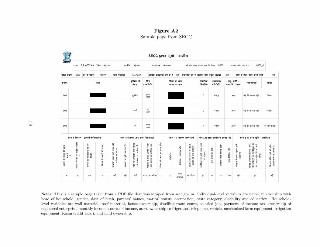
website (http://omms.nic.in), which we scraped in January 2015. Household microdata

comes from the Socioeconomic and Caste Census (SECC) of 2012, which describes every

household and individual in India. This dataset was collected by the Government of India

to determine eligibility for social programs. It was made publicly available on the internet

in a combination of formats; we scraped and processed over two million files covering 825

million rural individuals. After extracting text from the PDF tables, we translated fields

from various languages into English, classified occupations into standardized categories and

matched locations to the 2011 Population Census based on names. This process yielded a

range of variables covering both household characteristics (assets and income) and individual

characteristics (age, gender, occupation, caste, etc). Anonymized microdata from the 2002

Below Poverty Line (BPL) Census, an earlier national asset census, was used to construct

village level controls.

6Source: PMGSY administrative data. This figure describes the total amount disbursed by the end of2015. The cost per village connected is approximately $150,000.

9

To generate a measure of consumption, which is not directly surveyed by the SECC,

we predict consumption in a district-level survey (IHDS-II, 2011-12) that contains the same

asset, income and land data as the SECC. We then impute consumption for each individual in

the sample following the small area estimation methodology of Elbers et al. (2003), allowing

us to test not only for impacts of roads on mean consumption but also for distributional

effects.7 Appendix A contains additional details of this process.

Firm data comes from the Sixth Economic Census (2013). This covers every non-crop

producing economic establishment in India, including public and informal establishments. It

contains detailed information on location (which we match to the 2011 Population Census),

employment, industry and a handful of other firm characteristics, but includes no variables

on wages, inputs or outputs. We trim outliers to eliminate villages where the number of

workers in village nonfarm firms is greater than the total number of workers resident in the

village. Results are not substantively changed by this restriction.

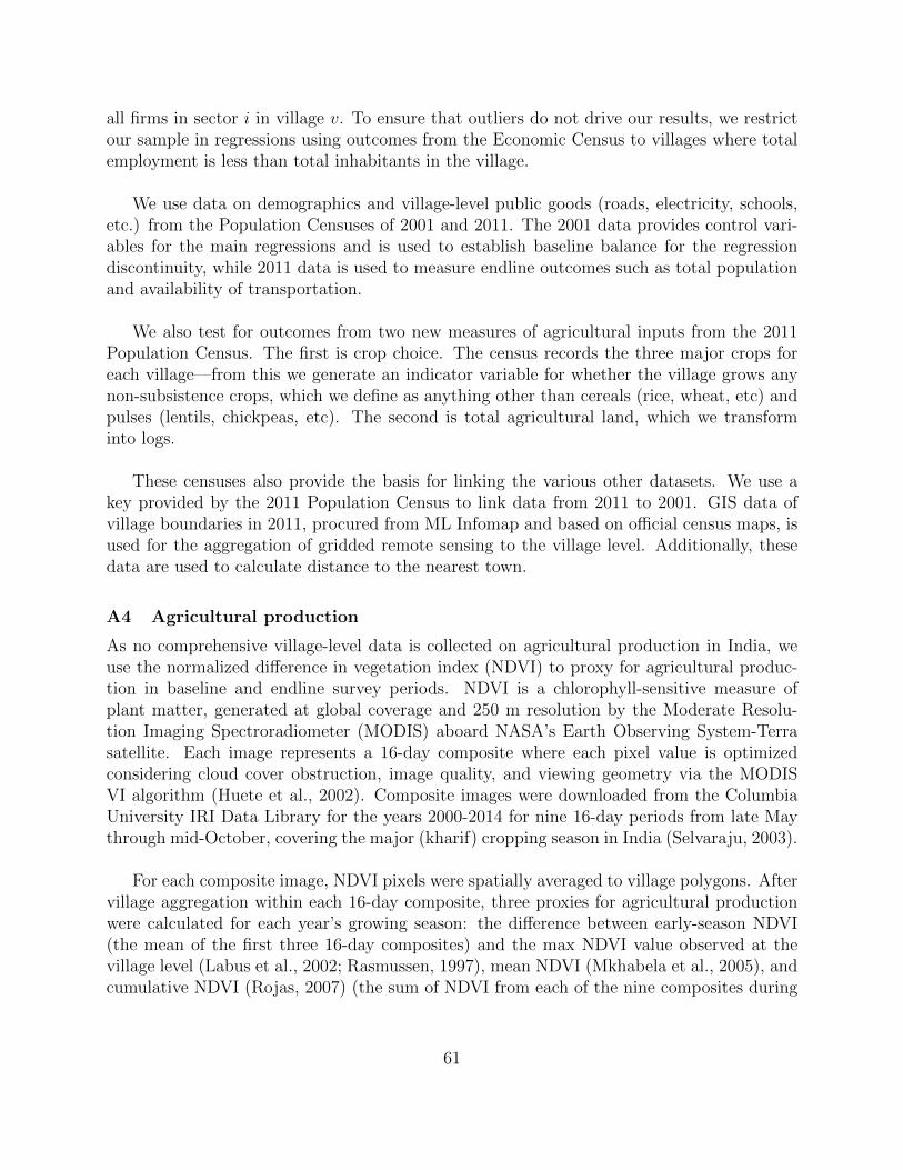
Remote sensing data is used to measure outcomes otherwise unavailable at the village

level. Nights lights provide a proxy for total village output. As no village-level agricultural

output data exists in India, we use a satellite-based vegetative index (NDVI) for the primary

(kharif) growing season (late May - October) to proxy for village-level agricultural produc-

tion. To control for differences in non-crop vegetation, we measure the maximum growing

season vegetation minus early cropping season vegetation.8 We use village boundary poly-

gons purchased from ML Infomap to map gridded remote sensing data to villages and to

determine treatment spillover catchment areas.

The 2001 and 2011 Population Censuses provide village infrastructure, demographics,

transportation services and the running variable for the regression discontinuity design (pop-

7Standard errors for all imputed consumption and poverty regressions are produced using the bootstrap-ping procedure outlined in Elbers et al. (2003).

8Table A1 shows that this measure is highly correlated with two other proxies for agricultural productivityand per capita consumption at the village level, as well as annual agricultural output at the district level.See Appendix A for additional details.

10

ulation in 2001). The 2011 Population Census also describes the three primary crops grown

in each village; we consolidate these into an indicator for whether one out of the three is

something other than a cereal (rice, wheat, etc) or pulse (lentils, chickpeas). The Population

Censuses also provide the basis for linking all other datasets together at the village level.

Figure 1 provides a visual representation of the timing of the major datasets used in this

project, along with year-by-year counts of the number of villages receiving PMGSY roads

for the years of this study. Road construction is negligible before baseline data collection

in 2001, then slowly ramps up to a peak of over 11,000 roads constructed annually in 2008

before slowing down slightly.

The analysis sample is restricted to the 11,474 villages that (i) did not have a paved road

in 2001; (ii) we were able to match across all primary datasets; and (iii) had populations

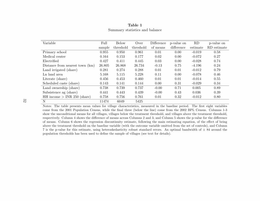
within the optimal bandwidth from a treatment threshold. Column 1 of Table 1 reports the

average characteristics of the villages in the sample; they are very similar to the average

unconnected village in India.9

V Empirical Strategy

The impacts of infrastructure investments are challenging for economists to measure for

several reasons. First, the high cost and large potential returns of such investments mean

that few policymakers are willing to allow random allocation. Political favoritism, economic

potential and pro-poor targeting would lead infrastructure to be correlated with other gov-

ernment programs and economic growth, biasing naive estimates in an unknown direction.

Second, because roads are costly, road construction programs rarely generate large treatment

samples. Sample surveys not directly connected with road construction programs are thus

unlikely to have a sufficient number of treated and control groups; in contrast, analysis at

9Table A2 shows village-level summary statistics for all villages in the 2001 Population Census, separatedinto those with and without roads. Villages without paved roads (which comprise nearly half of of all villages)are less populated (731 vs 1708), have fewer public goods (e.g. 26% electrified vs 55%), have less irrigatedagricultural land and are farther from the nearest urban center than villages with paved roads. The extentto which differences like these are endogenous or causal is the central question of this paper.

11

more aggregate levels is underpowered and faces greater identification concerns. We address

these challenges by combining quasirandom variation from program rules with administrative

census data georeferenced to the village level.

We obtain causal identification from the guidelines by which villages were prioritized to

receive new roads. As previously described, new roads were targeted first to villages with

population greater than 1000, then those greater than 500, and finally greater than 250.

While selection into road treatment may have been partly determined by political or economic

factors, these factors do not change discontinuously at these population thresholds. As long

as these rules were followed to any degree, the likelihood of treatment will discontinuously

increase at these population thresholds, making it possible to estimate the effect of new roads

using a fuzzy regression discontinuity design.

We pool villages according to the population thresholds that were applied in each state,

so the running variable is village population minus the treatment threshold. Very few villages

around the 250-person threshold received roads by 2012, so we limit the sample to villages

with populations close to 500 and 1000. Further, only certain states followed the population

threshold prioritization rules as given by the national guidelines of the PMGSY. We worked

closely with the National Rural Roads Development Agency to identify the state-specific

thresholds that were followed and we define our sample accordingly. Our sample is comprised

of villages from the following states, with the population thresholds used in parentheses:

Chhattisgarh (500, 1000), Gujarat (500), Madhya Pradesh (500, 1000), Maharashtra (500),

Orissa (500), and Rajasthan (500).10

Under the assumption of continuity of all other village characteristics other than road

treatment at the treatment threshold, the fuzzy RD estimator calculates the local average

treatment effect (LATE) of receiving a new road for a village with population equal to the

10These states are concentrated in north India. Southern states generally have far superior infrastructureand thus had few unconnected villages to prioritize. Other states such as Bihar had many unconnectedvillages but did not comply with program guidelines.

12

threshold. Following the recommendations of Imbens and Lemieux (2008) and Gelman and

Imbens (2017), our primary specification uses local linear regression within a given band-

width of the treatment threshold, and controls for the running variable (village population)

on either side of the threshold. We use the following two stage instrumental variables speci-

fication:

Roadv,j = γ0 + γ11{popv,j ≥ T}+ γ2(popv,j − T )+

γ3(popv,j − T ) ∗ 1{popv,j ≥ T}+ νXv,j + µj + υv,j

(1)

Yv,j = β0 + β1Roadv,j+β2(popv,j − T )+

β3(popv,j − T ) ∗ 1{popv,j ≥ T}+ ζXv,j + ηj + εv,j.

(2)

Yv,j is the outcome of interest in village v and group j, T is the population threshold,

popv,j is baseline village population, Xv,j is a vector of village controls measured at baseline,

and ηj and µj are district-threshold fixed effects. Village-level controls include indicators

for presence of village amenities (primary school, medical center and electrification), the

log of total agricultural land area, the share of agricultural land that is irrigated, distance

in km from the closest census town, the share of workers in agriculture, the literacy rate,

the share of inhabitants that belong to a scheduled caste, the share of households owning

agricultural land, the share of households who are subsistence farmers, and the share of

households earning over 250 INR cash per month (approximately 4 USD), all measured at

baseline. District-threshold fixed effects are district fixed effects interacted with an indicator

variable for whether the village is in the 1000-person threshold group. Roadv,j is an indicator

that takes the value one if the village received a new road before the year in which Y is

13

measured, which is 2011, 2012, or 2013 (depending on the data source).11 Village controls and

fixed effects are not necessary for identification but improve the efficiency of the estimation.

The coefficient β1 captures the effect of a new road on the outcome variable. The optimal

bandwidth according to the method of Imbens and Kalyanaraman (2012) is 84.12 We use a

triangular kernel which places the most weight on observations close to the threshold, as in

Dell (2015). Results are highly similar with different fixed effects or controls, a rectangular

kernel, or alternate bandwidths.

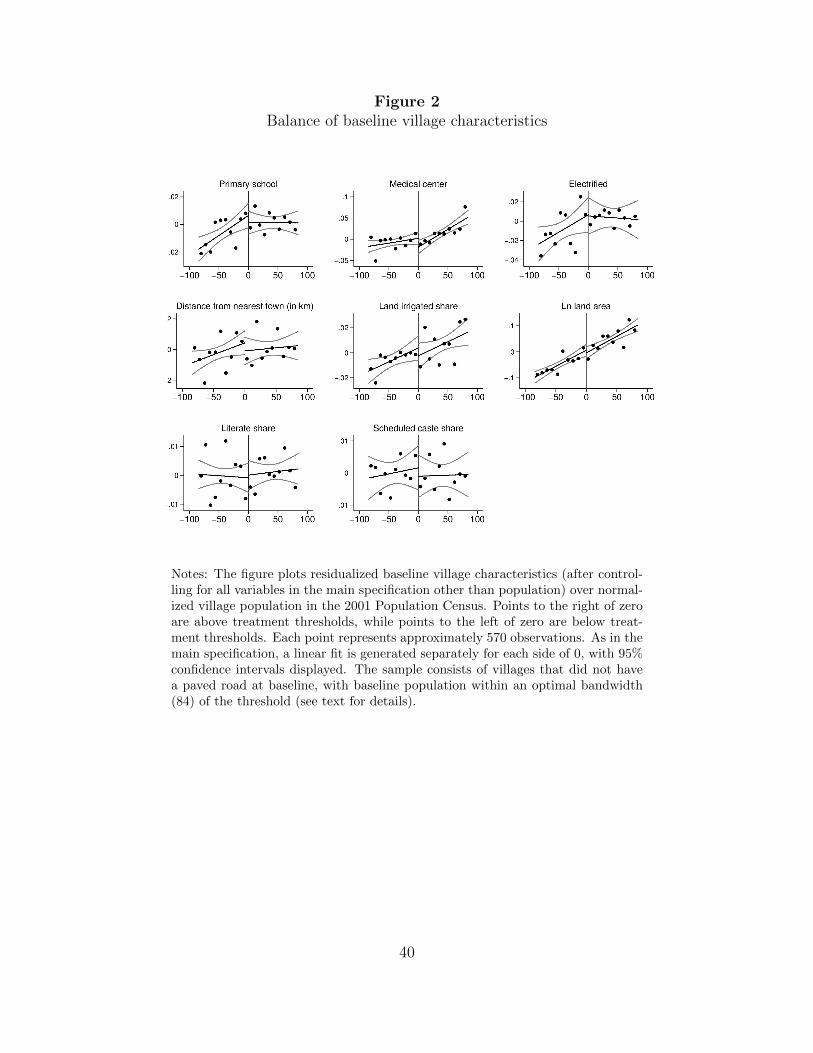
Regression discontinuity estimates can be interpreted causally if baseline covariates and

the density of the running variable are balanced across the treatment threshold. Table 1

presents the mean values for various village baseline characteristics, including the set of

controls that we use in all regressions. While there are average differences between villages

above and below the population threshold (Columns 2 and 3), in part because many village

characteristics are correlated with size, we find no significant differences when we use the

RD specification to test for discontinuous changes at the threshold. Figure 2 shows the

graphical version of the balance test, plotting means of baseline variables in population bins,

residual of fixed effects and controls. Baseline village characteristics are continuous at the

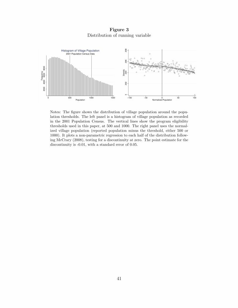
treatment threshold. Figure 3 shows that the density of the village population distribution

is also continuous across the treatment threshold; the McCrary test statistic is -0.01 (s.e.

0.05) (McCrary, 2008).13

11Our primary outcomes are measured in 2011 (Population Census), 2012 (SECC), and 2013 (EconomicCensus). These were not particularly unusual years for the Indian economy. GDP growth these years was6.6%, 5.5% and 6.4%, slightly below the 2008-16 average of 7.1%. Rainfall for the main growing season(June-September) was neither particularly high or low: 901, 824 and 937 mm, compared to the 2000-2014average of 848 mm.

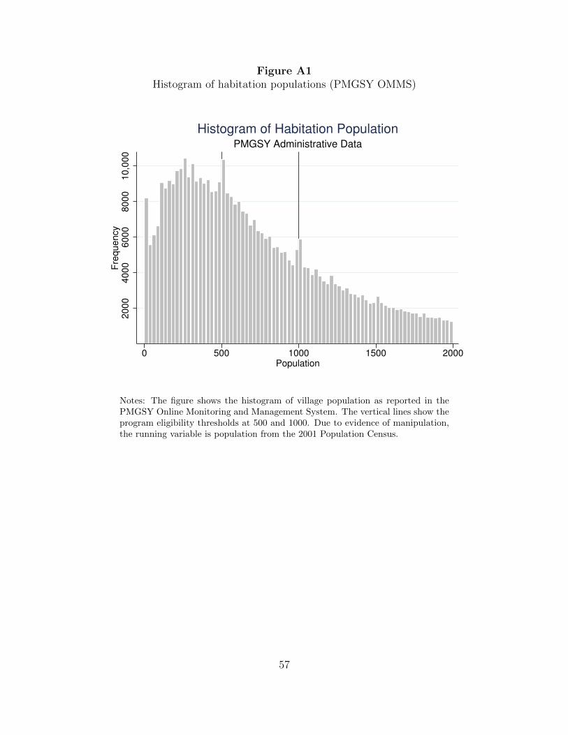
12The optimal bandwidth according to the method of Calonico et al. (2014) is 78.13Note that the density function of habitation population as reported in the internal PMGSY records

exhibits notable discontinuities above the treatment thresholds, indicating that some habitation were ableto misreport population to gain eligibility (Figure A1). For this reason, we use village population fromthe 2001 Population Census as the running variable. The Population Census was collected before PMGSYimplementation began to scale up, and was done so by a government agency considered to be apolitical andimpartial.

14

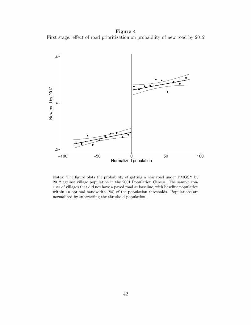
Figure 4 shows the share of villages that received new roads before 2012 in each population

band relative to the treatment threshold; there is a substantial discontinuous increase in the

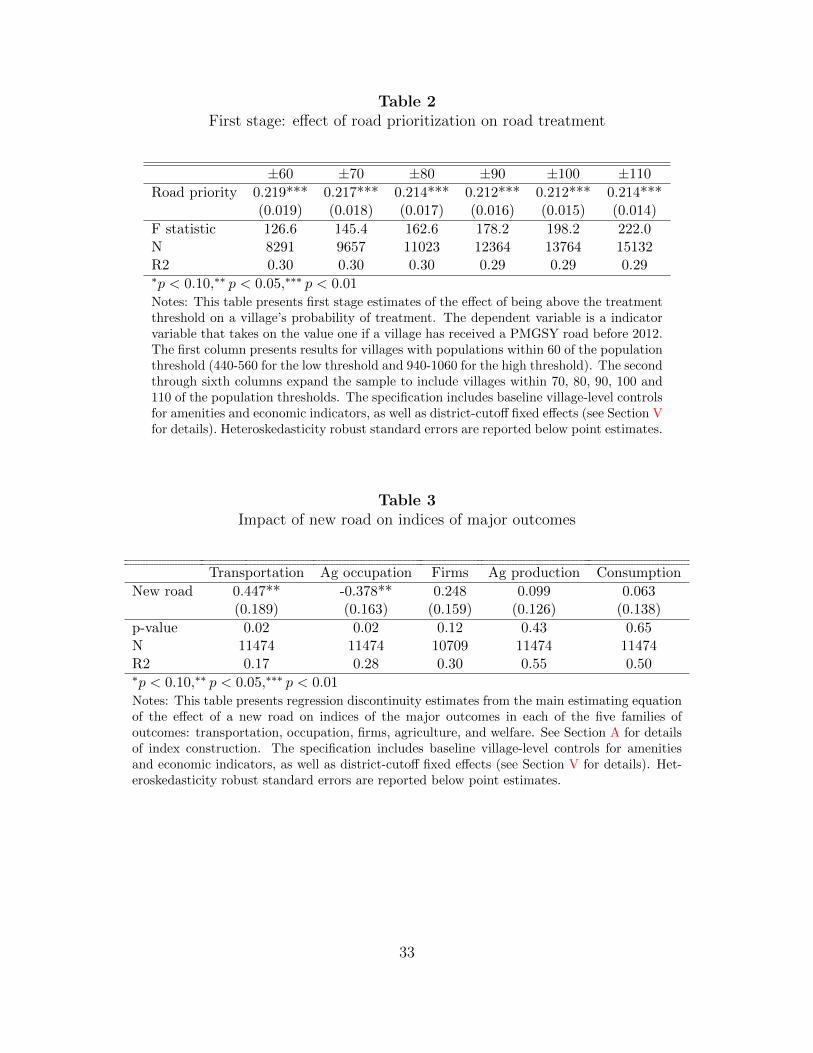
probability of treatment at the threshold. Table 2 presents first stage estimates using the

main estimating equation at various bandwidths. Crossing the treatment threshold raises

the probability of treatment by 21-22 percentage points; as suggested by the figure, the

estimates are very robust to different bandwidth choices.

VI Results

VI.A Main results

To summarize the results, we begin by presenting treatment estimates on five indices of

the major families of outcomes: (i) transportation services; (ii) sectoral allocation of labor;

(iii) employment in nonfarm village firms; (iv) agricultural investment and yields; and (v)

income, assets and consumption. We generate these indices to have a mean of 0 and a

standard deviation of 1, following Anderson (2008); the variables that make up each index

are described in the Data Appendix (Section A7). Table 3 presents the RD estimate of the

impact of roads on each outcome. The first column shows a large positive effect on the

availability of transportation services, and the second shows that roads cause a significant

reallocation of labor out of agriculture. We find an almost significant positive effect (p =

0.12) on employment growth in village firms (Column 3), but small and insignificant positive

effects on agricultural yields/investments and on the consumption index (Columns 4 and 5).

These indices address concerns about multiple hypothesis testing within families of outcomes.

To correct for cross-family multiple hypothesis testing, we follow the step-down procedure of

Benjamini and Hochberg (1995), which allows us to reject the null hypothesis of zero effect

on both transportation and agricultural labor share with a false discovery rate (adjusted

p-value) of 0.05.

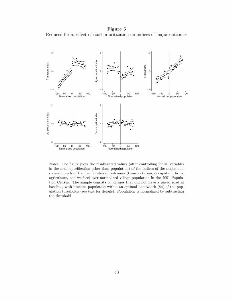
Figure 5 presents graphical representations of each column, showing the average of each

15

index as a function of distance from the treatment threshold. The plots show residuals from

controls and fixed effects, along with linear estimations on each side of the threshold and

95% confidence intervals. The graphs corroborate the tables, showing significant treatment

effects for transportation and labor exit from agriculture, but little clear impact on the

firms, agricultural production and consumption indices. These results broadly summarize

the findings of these paper: rural roads lead to increases in transportation services and

reallocation of labor out of agriculture, but no major changes to village firms, agricultural

production and consumption. The rest of this section examines the components of each

of these indices to explain the impacts of roads in more detail, and presents results on

heterogeneity.

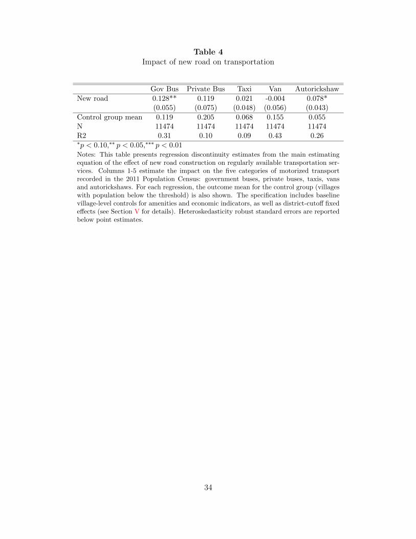
Table 4 shows regression discontinuity estimates of the impact of a new road on an indica-

tor variable for the regular availability at the village level of the five motorized transportation

services that are recorded in the 2011 Population Census. A new road causes a statistically

significant 12.8 percentage point increase in the availability of public bus services, more than

doubling the control group mean of 11.9 percent. The impact on private buses is nearly as

large but measured with less precision. Taxis and vans, which are more expensive forms

of transportation, do not experience significant growth. Availability of auto-rickshaws, the

least expensive private form of motorized transport, increases as well. Given that we are un-

able to observe transportation costs directly, we interpret these results as evidence that the

new roads studied in this paper do meaningfully affect connections between treated villages

and outside markets.14

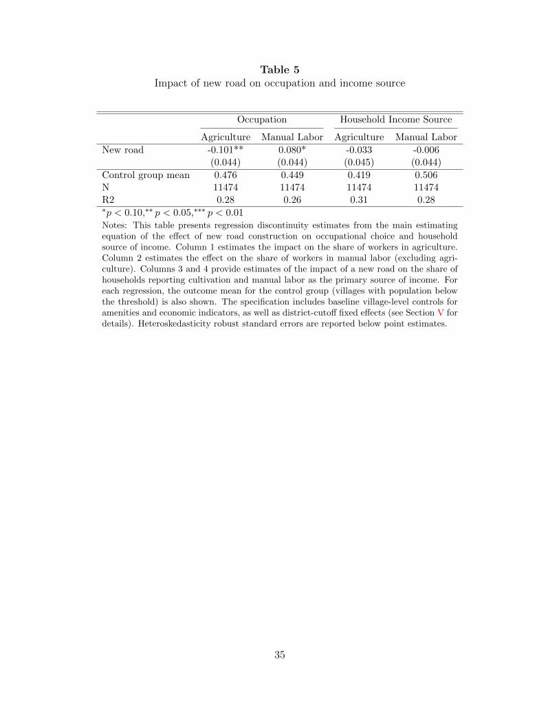
Table 5 presents impacts of new roads on occupational choice, the one domain where

roads appear to substantially change economic behavior. As 92% of workers in sample

villages report their occupation to be either in agriculture or in manual labor, we focus our

14This finding is not a given; Raballand et al. (2011) argue that in remote areas of Malawi, willingnessto pay for transportation services may be so low that roads may not appreciably improve transportationoptions.

16

investigation on these categories. The first two columns show the impact of new roads on the

share of workers (aged 21-60) who work in agriculture, and who work as manual laborers.

New roads cause a 10.1 percentage point reduction in workers in agriculture (representing a

21% decrease from the control group mean) and an 8.0 percentage point increase in workers

in (non-agricultural) manual labor.15 Columns 3 and 4 report estimates on the share of

households deriving their primary source of income from cultivation and manual labor. In

contrast to worker-level estimates, these regressions demonstrate that household income

source does not change significantly, suggesting that many of the workers exiting agriculture

are not the primary earners in the household. This result is also consistent with the finding

that consumption and income do not change dramatically in response to new roads.

Theoretically, we should expect those who exit agriculture in favor of nonfarm labor

market opportunities will be those for whom the losses of agricultural income are smallest

and the labor market gains are largest. By using individual-level census data, we can examine

the distribution of treatment effects across subgroups with different factor endowments. As

land is the major input into agricultural production, land endowments may play a major role

in determining which workers respond most to a rural road. We first examine the impact of

road construction on the landholding distribution in Table A4. We find that a new road does

not significantly change the share of households that are landless, own less than 2 acres, or

have between 2 and 4 acres of agricultural land. However, we do find a 3.4 percentage point

increase in the share of households with over four acres of land (significant at the 10 percent

level). We are hesitant to over-interpret one marginally significant result out of four tests,

but it is possible that there is some land consolidation following the construction of a road.

Regardless, we do not find major changes in the landholding distribution and thus treat

15The SECC does not report manual labor occupations in more detail. Table A3 breaks down the sectoraldistribution of non-agricultural manual laborers using the 68th round of the National Sample Survey (2011-12). By far the most common category of manual labor in India is construction, making it a likely sector formany of these former agricultural workers.

17

ex post observed landholdings as a baseline variable upon which to conduct heterogeneity

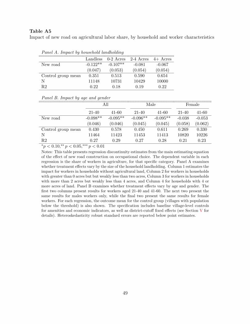
analysis. Panel A of Table A5 presents our main specification, estimating the effect on

agricultural occupation share separately by size of landholdings. We find that movement

out of agriculture is strongest for workers in households without land, and that this effect is

monotonically decreasing in landholding size.16 The decrease in agriculture for those with

no land (12.2 percentage points) is even larger as a percentage of the control group mean:

our estimates suggest that 35% of workers with no land exit agriculture, compared to just

10% in households with more than four acres of land.17 These results are consistent with

recent work finding that the inheritance of land in India can significantly reduce rates of

migration and participation in non-agricultural occupations (Fernando, 2016) and suggest

that the lack of transport infrastructure may be one cause of the inefficiently small size of

many farms in rural India (Foster and Rosenzweig, 2011).18

We next examine the heterogeneity of the treatment effect as a function of age and gender

(Table A5, Panel B). There are no differential results by age: the point estimate for workers

aged 21-40 (a 9.8 percentage point decrease in the share in agriculture) is almost identical

to the effect for workers aged 41-60 (a 9.5 percentage point decrease). While the differences

are not significantly different, we do find that men are more likely to exit agriculture as

compared to women, particularly in the younger cohort (-9.6 percentage point effect for

men compared to -3.8 percentage point for women). These estimates could be the result of

a male physical advantage in non-agricultural work or attitudes against women’s working

far away from home that may prevent reallocation of female labor away from agriculture

16We cannot statistically reject equality between any of these estimates. It is also possible that the observedheterogeneity may be affected by the small shift in the distribution of landholdings.

17It is important to note that productivity in agriculture will only depend on landholdings if there aremarket failures such that it is more productive to work on one’s own land. An extensive literature investigatescommon failures in agricultural land and labor markets in low income countries. See, for example, de Janvryet al. (1991).

18These effects also suggest that new roads may be a progressive investment in that those with the leastagricultural wealth (as proxied by landholding) show the largest labor market effects.

18

(Goldin, 1995). However, as a percentage of the control group mean, the estimates for male

and female workers are much closer.

Table 6 presents results on employment in village firms; Panel A shows estimates in

logs and Panel B in levels. Because the data source is the Economic Census, these counts

include all work in the village, formal and informal, excluding crop production. These

results capture economic activity that takes places in the village, in contrast to Table 5,

which describes economic activities for village residents even if they take place outside the

village. We present estimates for total non-farm village employment (Column 1), as well as

employment in the five largest sectors in the sample (livestock, manufacturing, education,

retail and forestry), which together account for 79% of non-farm employment. We estimate

an insignificant 25 percent increase in employment in non-farm firms. While the two largest

village sectors (livestock and manufacturing) show similarly growth to total employment, the

only statistically significant estimate we find is for retail, which we estimate grows 34 percent

in response to a new road. In levels, we find no significant results overall or in any sector,

with estimates ranging from 1.6 jobs lost in livestock to 2.6 jobs gained in manufacturing.

While the log changes in employment are quite large, the level changes are small because

the typical 500- or 1000-person village has few people engaged in economic activities other

than crop production. We estimate that a new road on average creates 3.7 new jobs in

a village. In contrast, the estimate from Table 5 suggest that 18.5 workers are exiting

agriculture in the average village; only 20% of these workers appear to be finding this non-

agricultural work in the village. These small impacts on firms imply that roads are facilitating

access to external labor markets rather than growth of jobs in village firms. The proportional

changes are the largest in the retail sector, suggesting that non-farm employment growth

in the village may be more a function of new consumption opportunities (perhaps due to

cheaper imports) rather than new productive opportunities. Unfortunately we are aware of

no village-level data that would make it possible to directly test for changes in the availability

19

or prices of consumption goods.

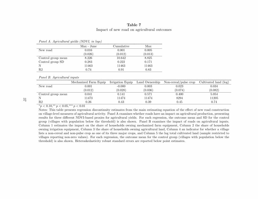
In Table 7, we examine whether new roads increase investments in agriculture or agri-

cultural yields. Panel A presents the impact of roads on the three different remotely sensed

proxies of yield, described in Section IV. Point estimates are very close to zero and the

standard errors are tight. In our preferred measure, we estimate an impact of 1.6% higher

agricultural yield (equivalent to 0.057 SD) and can rule out a 6.7% or a 0.24 standard devi-

ation increase in yield with 95% confidence.

In Panel B, we examine agricultural input usage. We find no evidence for increases in

ownership of mechanized farm or irrigation equipment. There is also no indication of a

movement away from subsistence crops, of land extensification, or of changes in the distribu-

tion of land ownership. In short, we find no evidence of substantial changes in agricultural

production in villages after they receive new roads. Our measures are admittedly incom-

plete and we are not able to measure agricultural output directly, but the zero effects for all

these different correlates of agricultural production suggest that the structure of agricultural

production is not dramatically affected by these new roads.

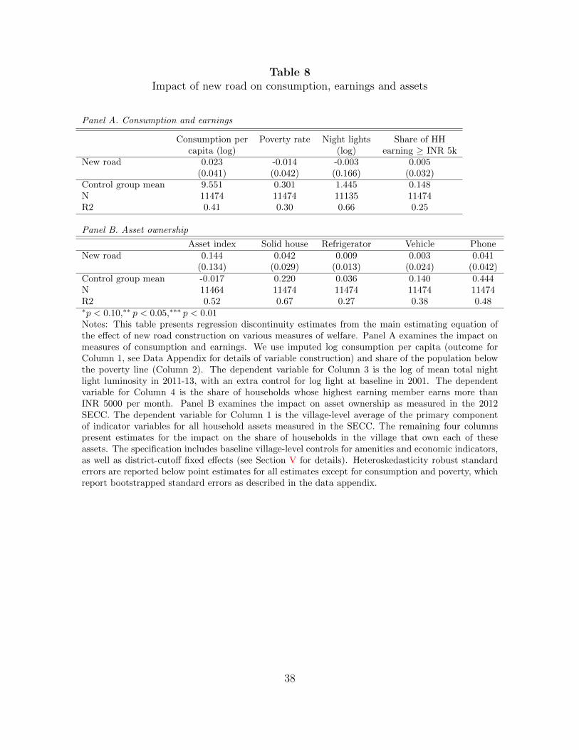
Finally, in Table 8, we examine the impact of roads on consumption, earnings and assets,

which are the best available measures of whether these roads make people appreciably better

off in villages. Panel A reports impacts on various measures of consumption and income. We

estimate that roads cause a statistically insignificant 2% increase in consumption; we can

rule out a 10% increase in consumption with 95% confidence. Because we can calculate the

consumption measure for every individual in every village, we can further estimate changes

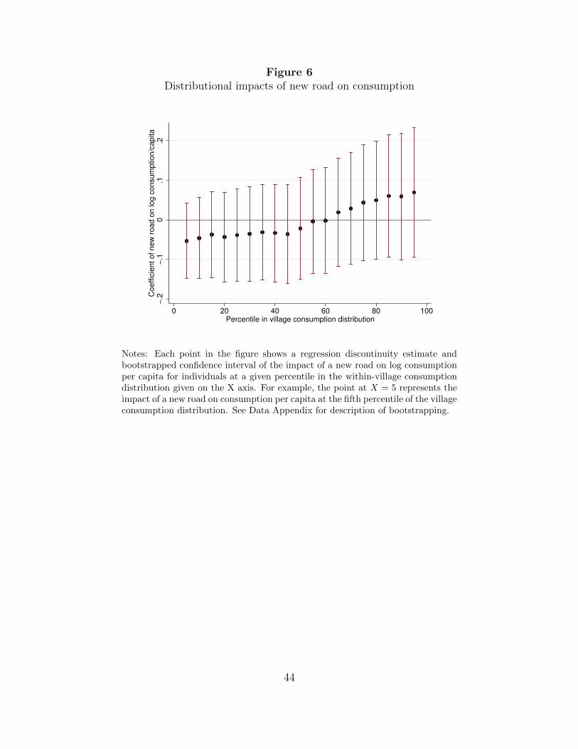
in consumption at any percentile of the village consumption distribution. Figure 6 shows RD

estimates at every ventile of the within-village consumption distribution; effects are weakly

more positive at the top of the consumption distribution, but very small and insignificant

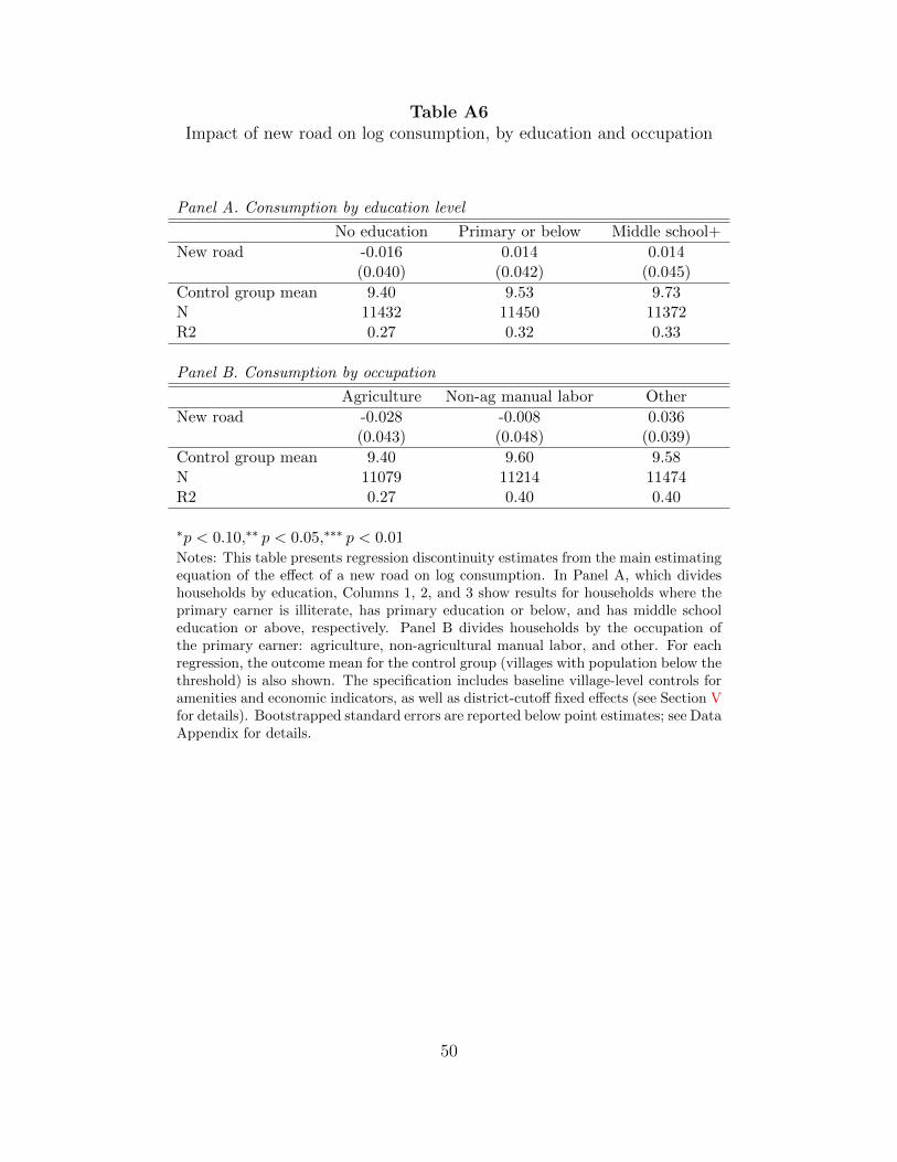
everywhere. Table A6 separates consumption estimates by education and occupation of the

20

household head; there are no significant consumption gains in any of the categories.19

Log night light intensity at the village level (Table 8, Column 3) provides an alternative

measure of consumption (Henderson et al., 2011); we again find a point estimate very close

to zero. Finally, Column 4 shows estimates on the share of households in the village whose

primary earner makes more than 5,000 rupees (approximately $100) per month.20 Once

again, we find no statistically or economically significant effect; the coefficient is comparable

to the consumption proxy.

Panel B of Table 8 estimates the impact of new roads on asset ownership. The normalized

asset index suggests a small and statistically insignificant 0.14 standard deviation increase

in assets. The remaining columns show small and insignificant estimates on ownership of the

assets that make up the index. All evidence suggests that rural roads do not greatly increase

earnings, assets, or consumption, even for relatively inexpensive assets such as mobile phones.

To summarize, new roads do not appear to substantially change either the aggregate

economy or consumption in connected villages. We do observe a substantial shift of workers

out of agricultural work and into wage work, but these individuals tend not to be the primary

household earners, and this occupational change does not lead to substantial changes in

income or consumption. The average treated village has had a road for 4 years at the time

of measurement in 2012. Given the small positive point estimates on the consumption and

agricultural investment indices, it is possible that long-run effects are larger. But the results

do not paint a picture of villages poised to reap large benefits from improved transportation

infrastructure in the medium run.

19Note that we measure occupation of the household head in 2012, so some share of the household headsworking for wages may be doing so as a result of the treatment.

20As noted in Section A, the SECC reports income only in three bins and only for the highest earner ofthe household, so we do not have a more granular measure.

21

VI.B Robustness

In this section we examine the robustness of our results to alternative specifications and

explanations.

First, as a placebo exercise, we estimate the first stage and reduced form estimation on the

family indices for the set of states that did not follow guidelines regarding the population

eligibility threshold. If villages above the PMGSY thresholds are changing in ways other

than through eligibility for roads, we would expect to find similar reduced form effects in

these placebo villages as well. Specifically, we include villages close to the two population

thresholds in states that built many roads but did not follow the rules at all (Andhra Pradesh,

Assam, Bihar, Jharkhand, Karnataka, Uttar Pradesh and Uttarakhand), and villages close to

the 1000 threshold in states that used only the 500-person threshold (Gujarat, Maharashtra,

Orissa and Rajasthan). Table A7 presents the estimates. There is no evidence of either a

first stage or reduced form effect on any outcomes in the placebo sample, suggesting that

our primary estimates can indeed be interpreted as resulting from new roads.

In Table A8, we present the five family index results for bandwidths from 60 to 100, for

both triangular and rectangular kernels. The results are consistent with the those in our

main specification (Table 3).

If rural roads are causing selective migration, as some studies on transport costs have

found (Bryan et al., 2014; Morten and Oliveira, 2017), compositional changes in village pop-

ulation could bias treatment estimates. In Table A9, we examine three proxies for permanent

migration.21 First we test for impacts on village population in 2011 (Panel A). We find no

evidence for significant impacts on total population, either in logs or levels. The limitation

of population growth as an outcome is that any impacts on net migration could be offset by

changes to fertility and mortality. But such offsetting effects would causes changes in village

21Short-term migrants and commuters are considered resident in the village, and thus covered in both thePopulation Censuses and the SECC.

22

demographics, which we can estimate in the comprehensive census data. In Panels B and

C, we show that roads cause no changes to the age distribution or gender ratios in any age

cohort. Taken together, these three pieces of evidence suggest that new roads do not lead to

major changes in out-migration.22 The absence of an impact on migration also allows us to

interpret the observed sectoral reallocation of labor as the result of changes in occupational

choice rather than compositional effects due to selective migration.

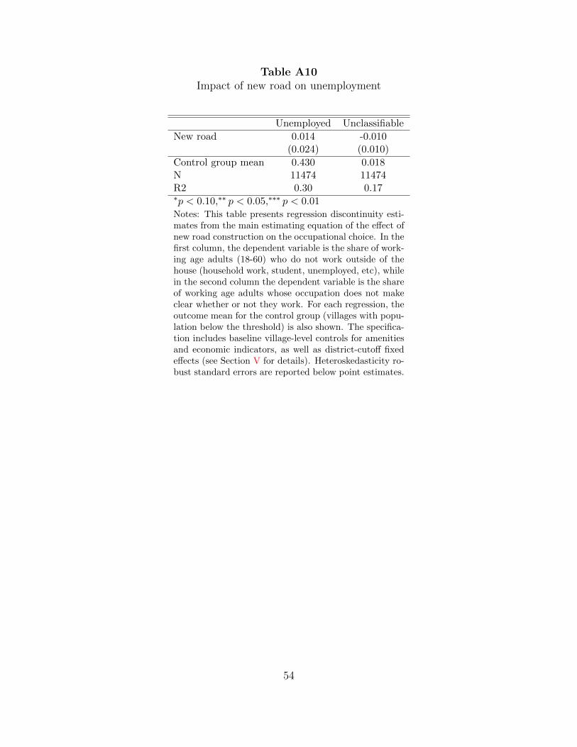
Table A10 addresses the possibility that the workforce has changed, which would make it

difficult to interpret changes in the share of workers in agriculture or non-agricultural wage

work. The table shows that roads do not affect the share of adults who are either not working

or who are in occupations that we are unable to classify, suggesting that this potential bias

is not important.

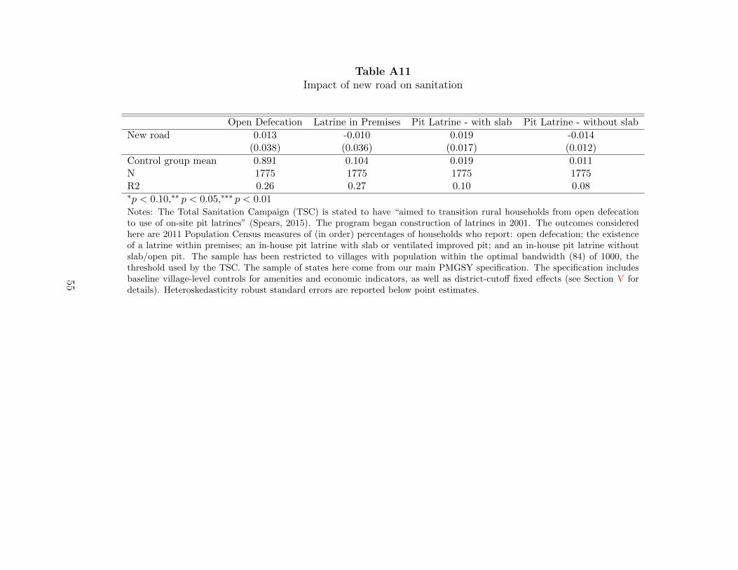
A different threat to our identification could come from any other policy that used the

same thresholds as the PMGSY. In fact, one national government program did prioritize

villages above population 1000: the Total Sanitation Campaign (Spears, 2015), which at-

tempted to reduce open defecation through toilet construction and advocacy. It is unlikely

that this program is spuriously driving our results for two reasons. First, there is little

theoretical reason to believe that investments in sanitation could drive large increases in

transportation services or reallocation of labor away from agriculture. Second, in Table A11

we present regression discontinuity estimates of the impact of road prioritization on four

measures of sanitation. We find no evidence that being above the population threshold is

associated either with open defecation or any measure of access to toilets, suggesting that

there is no discontinuity in the implementation of the program that might affect our results.

Finally, we consider the possibility that roads have spillover effects on nearby villages; if

22This difference with Morten and Oliveira (2017) may be due to the differences between rural feeder roadsand highways. The construction of a paved rural road is unlikely to significantly change the one-time cost ofpermanent migration relative to the lifetime benefits, in contrast to the major changes induced by highwayconstruction.

23

so, our estimates of direct effects could be biased either upwards or downwards relative to

the total effects of new road provision. To do so, we examine outcomes in villages within

a 5 km radius of villages in the main sample, using the standard regression discontinuity

specification. Table A12 presents results of these regressions for the outcome family indices.

We find no evidence of spillovers, and can reject equality with the main point estimates on

the transportation and agricultural occupation measures.

VII Conclusion

A large share of the world’s poor are in rural areas without access to the paved road network.

The resulting high transportation costs potentially inhibit gains from the division of labor,

economies of scale and specialization.

In this paper we estimate the economic impacts of the Pradhan Mantri Gram Sadak

Yojana, a large-scale program in India that seeks to provide universal access to paved “all-

weather” roads in rural India. We exploit discontinuities in the probability of paved road

construction at village population thresholds, finding that rural roads do not substantially

change village economies. In agriculture, the largest sector in rural India, these roads af-

fect neither input usage nor output. We do find that new paved roads lead to increased

transportation services and a large reallocation of labor out of agriculture. But rather than

causing nonfarm growth in rural areas, roads appear to facilitate the access of rural labor to

external employment.

Roads are costly investments: the cost of connecting each village to the paved road

network is approximately $150,000. In contrast to expectations that these roads would

boost income and reduce poverty, we find insignificant and small effects on earnings and

consumption. In our sample, the mean consumption per capita is approximately $267 per

year and the average village has 696 inhabitants. We estimate an increase in consumption of

2.3%, which translates into $6.14 additional annual consumption per person, or only $4274

24

per year for the village as a whole. Even if we use the upper bound of the confidence interval

on consumption, we find small effects relative to the cost of roads. This number appears

even smaller when one considers that roads require costly ongoing maintenance. Worse yet,

the villages in India still lacking paved roads are less populated and more remote than those

in our sample, suggesting that impacts for future rural road investments are likely to be

even smaller. This said, rural roads may have other indirect positive effects that we have

not measured here, such as increasing schooling or access to health services.

Both researchers and policymakers have suggested that roads have the potential to revolu-

tionize economic opportunity in remote, rural areas. In principle, roads could raise farmgate

prices and grow the nonfarm sector through trade with outside markets, boosting wages and

providing jobs. This paper suggests that even in a fast growing economy such as India in the

2000s, rural growth is constrained by more than the poor state of transportation infrastruc-

ture. Given the apparent difficulty of moving production to the hundreds of millions of rural

poor, there may be higher returns to facilitating their access to areas of high productivity

and opportunity.

25

References

Adukia, Anjali, Sam Asher, and Paul Novosad, “Educational Investment Responsesto Economic Opportunity: Evidence from Indian Road Construction,” 2017. Workingpaper.

Aggarwal, Shilpa, “Do Rural Roads Create Pathways out of Poverty? Evidence fromIndia,” 2017. Working Paper.

Ali, Rubaba, “Impact of Rural Road Improvement on High Yield Variety TechnologyAdoption: Evidence from Bangladesh,” 2011. Working paper.

Alkire, Sabina and Suman Seth, “Identifying BPL Households: A Comparison of Meth-ods,” Economic and Political Weekly, 2013, 48 (2), 49–57.

Anderson, Michael L., “Multiple Inference And Gender Differences In The Effects OfEarly Intervention: A Reevaluation Of The Abecedarian, Perry Preschool, And EarlyTraining Projects,” Journal of the American Statistical Association, 2008, 103 (484),1481–1495.

Atkin, David, Azam Chaudhry, Shamyla Chaudry, Amit K. Khandelwal, andEric Verhoogen, “Markup and Cost Dispersion across Firms: Direct Evidence fromProducer Surveys in Pakistan,” The American Economic Review, 2015, 105 (5). Work-ing Paper.

Banerjee, Abhijit, Esther Duflo, and Nancy Qian, “On the Road: Access to Trans-portation Infrastructure and Economic Growth in China,” 2012. NBER Working PaperNo. 17897.

Baum-Snow, Nathaniel, Loren Brandt, J. Vernon Henderson, and Matthew A.Turner, “Roads, Railroads and Decentralization of Chinese Cities,” Review of Eco-nomics and Statistics, 2017.

Benjamini, Yoav and Yosef Hochberg, “Controlling the False Discovery Rate: A Practi-cal and Powerful Approach to Multiple Testing,” Journal of the Royal Statistical Society.Series B (Methodological), 1995, 57 (1), 289–300.

Binswanger, Hans P., Shahidur R. Khandker, and Mark R. Rosenzweig, “HowInfrastructure and Financial Institutions Affect Agricultural Output and Investment inIndia,” Journal of Development Economics, 1993, 41 (2).

Blimpo, M. P., R. Harding, and L. Wantchekon, “Public Investment in Rural In-frastructure: Some Political Economy Considerations,” Journal of African Economies,2013, 22 (AERC Supplement 2).

Brueckner, Markus, “Infrastructure, Anocracy, and Economic Growth: Evidence fromInternational Oil Price Shocks,” 2014. Working paper.

26

Bryan, Gharad and Melanie Morten, “Economic Development and the Spatial Alloca-tion of Labor: Evidence From Indonesia,” 2015. Working paper.

, Shyamal Chowdury, and Ahmed Mushfiq Mobarak, “Underinvestment in aProfitable Technology: The Case of Seasonal Migration in Bangladesh,” Econometrica,2014, 82 (5).

Burgess, Robin and Dave Donaldson, “Railroads and the Demise of Famine in ColonialIndia,” 2012. Working paper.

, Remi Jedwab, Edward Miguel, Ameet Morjaria, and Gerard Padro iMiquel, “The Value of Democracy: Evidence from Road Building in Kenya,” AmericanEconomic Review, 2015, 105 (6).

Bustos, Paula, Bruno Caprettini, and Jacopo Ponticelli, “Agricultural Productiv-ity and Structural Transformation. Evidence from Brazil,” The American EconomicReview, 2016, 106 (6), 1320–1365.

Calonico, Sebastian, Matias D. Cattaneo, and Rocio Titiunik, “Robust Nonpara-metric Confidence Intervals for Regression-Discontinuity Designs,” Econometrica, 2014,82 (6), 2295–2326.

Casaburi, Lorenzo, Rachel Glennerster, and Tavneet Suri, “Rural Roads and Inter-mediated Trade: Regression Discontinuity Evidence from Sierra Leone,” 2013. WorkingPaper.

de Janvry, Alain, Marcel Fafchamps, and Elisabeth Sadoulet, “Peasant HouseholdBehaviour With Missing Markets: Some Paradoxes Explained,” The Economic Journal,1991, 101 (409), 1400–1417.

Dell, Melissa, “Trafficking Networks and the Mexican Drug War,” American EconomicReview, 2015, 105 (6).

Dercon, Stefan, Daniel O. Gilligan, John Hoddinott, and Tassew Woldehanna,“The Impact of Agricultural Extension and Roads on Poverty and Consumption Growthin Fifteen Ethiopian Villages,” American Journal of Agricultural Economics, 2009, 91(4), 1007–1021.

Dinkelman, Taryn, “The Effects of Rural Electrification on Employment: New Evidencefrom South Africa,” American Economic Review, 2011, 101 (7), 3078–3108.

Donaldson, Dave, “Railroads of the Raj: Estimating the Impact of Transportation Infras-tructure,” American Economic Review (forthcoming).

and Richard Hornbeck, “Railroads and American Economic Growth: A ”MarketAccess” Approach,” Quarterly Journal of Economics, 2016, 131 (2).

27

Duflo, Esther and Rohini Pande, “Dams,” Quarterly Journal of Economics, 2007, 122(2), 601–646.

Elbers, Chris, Jean Lanjouw, and Peter Lanjouw, “Micro-level Estimation of Povertyand Inequality,” Econometrica, 2003, 71 (1), 355–364.

Faber, Benjamin, “Trade Integration, Market Size, And Industrialization: Evidence FromChina’s National Trunk Highway System,” Review of Economic Studies, 2014, 81 (3).

Fafchamps, Marcel and Forhad Shilpi, “Cities and Specialisation: Evidence from SouthAsia,” The Economic Journal, 2005, 115 (503), 477–504.

Fan, Shenggen and Peter Hazell, “Returns to Public Investments in the Less-FavoredAreas of India and China,” American Journal of Agricultural Economics, 2001, 83 (5),1217–1222.

Fernando, A. Nilesh, “Shackled to the Soil: The Long-Term Effects of Inherited Land onLabor Mobility and Consumption,” 2016. Working paper.

Foster, Andrew D. and Mark R. Rosenzweig, “Are Indian Farms Too Small? Mecha-nization, Agency Costs, and Farm Efficiency,” 2011. Working paper.

Gelman, Andrew and Guido Imbens, “Why High-order Polynomials Should Not BeUsed in Regression Discontinuity Designs,” Journal of Business & Economic Statistics(accepted), 2017. NBER Working Paper No. 20405.

Ghani, Ejaz, Arti Grover Goswami, and William R. Kerr, “Highway to Success:The Impact of the Golden Quadrilateral Project for the Location and Performance ofIndian Manufacturing,” Economic Journal, 2015.

Gibson, John and Scott Rozelle, “Poverty and Access to Roads in Papua New Guinea,”Economic Development and Cultural Change, 2003, 52 (1), 159–185.

and Susan Olivia, “The Effect of Infrastructure Access and Quality on Non-farmEnterprises in Rural Indonesia,” World Development, 2010, 38 (5), 717–726.

Goldin, Claudia, “The U-shaped Female Labour Force Function in Economic Developmentand Economic History,” in T. Paul Schultz, ed., Investment in Women’s Human Capital,Chicago and London: University of Chicago Press, 1995.

Gollin, Douglas and Richard Rogerson, “Productivity, Transport Costs and SubsistenceAgriculture,” Journal of Development Economics, 2014, 107, 38–48.

, David Lagakos, and Michael E. Waugh, “The Agricultural Productivity Gap,”Quarterly Journal of Economics, 2014, 129 (2), 939–993.

28

Gonzalez-Navarro, Marco and Climent Quintana-Domeque, “Paving Streets forthe Poor: Experimental Analysis of Infrastructure Effects,” Review of Economics andStatistics, 2016, 98 (2), 254–267.

Henderson, Vernon, Adam Storeygard, and David N. Weil, “A Bright Idea forMeasuring Economic Growth,” American Economic Review, 2011, 101 (3).

Hicks, Joan Hamory, Marieke Kleemans, Nicholas Y. Li, and Edward Miguel,“Reevaluating Agricultural Productivity Gaps with Longitudinal Microdata,” 2017.NBER Working Paper No. 23253.

Huete, A., K. Didan, T. Miura, E. P. Rodriguez, X. Gao, and L. G. Ferreira,“Overview of the Radiometric and Biophysical Performance of the MODIS VegetationIndices,” Remote Sensing of Environment, 2002, 83 (1-2), 195–213.

Imbens, Guido and Karthik Kalyanaraman, “Optimal Bandwidth Choice for the Re-gression Discontinuity Estimator,” Review of Economic Studies, 2012, 79 (3).

and Thomas Lemieux, “Regression Discontinuity Designs: a Guide to Practice,”Journal of Econometrics, 2008, 142 (2), 615–635.

Jacoby, Hanan and Bart Minten, “On Measuring the Benefits of Lower TransportCosts,” Journal of Development Economics, 2009, 89, 28–38.

Jacoby, Hanan G., “Access to Markets and the Benefits of Rural Roads,” The EconomicJournal, 2000, 110 (465), 713–737.

Khandker, Shaidur R. and Gayatri B. Koolwal, “Estimating the Long-term Impacts ofRural Roads: A Dynamic Panel Approach,” 2011. World Bank Policy Research PaperNo. 5867.

, Zaid Bakht, and Gayatri B. Koolwal, “The Poverty Impact of Rural Roads:Evidence from Bangladesh,” Economic Development and Cultural Change, 2009, 57(4), 685–722.

Labus, M. P., G. A. Nielsen, R. L. Lawrence, R. Engel, and D. S. Long, “WheatYield Estimates Using Multi-temporal NDVI Satellite Imagery,” International Journalof Remote Sensing, jan 2002, 23 (20), 4169–4180.

Lehne, Jonathan, Jacob Shapiro, and Oliver Vanden Eynde, “Building Connec-tions: Political Corruption and Road Construction in India,” Journal of DevelopmentEconomics, 2018, 131, 62–78. Working paper.

Lipscomb, Molly, Ahmed Mushfiq Mobarak, and Tania Bahram, “DevelopmentEffects of Electrification: Evidence From the Geologic Placement of Hydropower Plantsin Brasil,” American Economic Journal: Applied Economics, 2013, 5 (2), 200–231.

29

McCrary, Justin, “Manipulation of the Running Variable in the Regression DiscontinuityDesign: a Density Test,” Journal of Econometrics, 2008, 142 (2), 698–714.

McMillan, Margaret, Dani Rodrik, and Inigo Verduzco-Gallo, “Globalization,Structural Change, and Productivity Growth, with an Update on Africa,” World De-velopment, 2014, 63, 11–32.

Mkhabela, Manasah S., Milton S. Mkhabela, and Nkosazana N. Mashinini, “EarlyMaize Yield Forecasting in the Four Agro-ecological Regions of Swaziland Using NDVIData Derived From NOAA’s-AVHRR,” Agricultural and Forest Meteorology, 2005, 129(1-2), 1–9.

Morten, Melanie and Jaqueline Oliveira, “The Effects of Roads on Trade and Mi-gration: Evidence from a Planned Capital City,” 2017. NBER Working Paper No.22158.

Mu, Ren and Dominique van de Walle, “Rural Roads and Local Market Developmentin Vietnam,” Journal of Development Studies, 2011, 47 (5).

Mukherjee, Mukta, “Do Better Roads Increase School Enrollment? Evidence from aUnique Road Policy in India,” 2012. Working paper.

Narayanan, K. R., “Address by President of India to Parliament,” 2001.

National Rural Roads Development Agency, “Pradhan Mantri Gram Sadak YojanaOperations Manual,” Technical Report, Ministry of Rural Development, Governmentof India 2005.

Raballand, Gael, Rebecca Thornton, Dean Yang, Jessica Goldberg, Niall Kele-her, and Annika Muller, “Are Rural Road Investments Alone Sufficient to GenerateTransport Flows? Lessons from a Randomized Experiment in Rural Malawi and PolicyImplications,” 2011.

Rasmussen, M. S., “Operational Yield Forecast Using AVHRR NDVI Data: Reduction ofEnvironmental and Inter-annual Variability,” International Journal of Remote Sensing,mar 1997, 18 (5), 1059–1077.

Redding, Stephen J. and Matthew A. Turner, “Transportation Costs and the SpatialOrganization of Economic Activity,” in “Handbook of Regional and Urban Economics,Vol. 5B” 2015, chapter 20.

Roberts, Peter, K. C. Shyam, and Cordula Rastogi, “Rural Access Index: A KeyDevelopment Indicator,” Technical Report, The World Bank 2006.

Rojas, O., “Operational Maize Yield Model Development and Validation Based on Re-mote Sensing and Agro-meteorological Data in Kenya,” International Journal of RemoteSensing, sep 2007, 28 (17), 3775–3793.

30

Selvaraju, R., “Impact of El Nino-southern Oscillation on Indian Foodgrain Production,”International Journal of Climatology, feb 2003, 23 (2), 187–206.

Shamdasani, Yogita, “Rural Road Infrastructure & Agricultural Production: Evidencefrom India,” 2016. Working paper.

Shrestha, Slesh A., “Roads, Participation in Markets, and Benefits to Agricultural House-holds: Evidence from the Topography-based Highway Network in Nepal,” 2017. Work-ing paper.

Sotelo, Sebastian, “Domestic Trade Frictions and Agriculture,” 2016. Working paper.

Spears, Dean, “Effects of Sanitation on Early-life Health: Evidence From a GovernanceIncentive in Rural India,” 2015. Working paper.

Storeygard, Adam, “Farther on Down the Road: Transport Costs, Trade and UrbanGrowth in Sub-saharan Africa,” Review of Economic Studies, 2016, 83 (3).

Wantchekon, Leonard, Marko Klasnja, and Natalija Novta, “Education and HumanCapital Externalities: Evidence from Benin,” The Quarterly Journal of Economics,2015, 130 (2), 703–757.

World Bank Group, “Measuring Rural Access Using new technologies,” 2016, p. 108.

Zhang, Xiaobo and Shenggen Fan, “How Productive is Infrastructure? A New Approachand Evidence from Rural India,” American Journal of Agricultural Economics, 2004,86 (2), 492–501.

31

Table 1Summary statistics and balance

Variable Full Below Over Difference p-value on RD p-value onsample threshold threshold of means difference estimate RD estimate

Primary school 0.955 0.950 0.961 0.01 0.00 -0.019 0.58Medical center 0.164 0.153 0.177 0.02 0.00 -0.072 0.27Electrified 0.427 0.411 0.445 0.03 0.00 -0.028 0.74Distance from nearest town (km) 26.805 26.868 26.734 -0.13 0.75 -4.196 0.24Land irrigated (share) 0.281 0.274 0.288 0.01 0.01 -0.012 0.79Ln land area 5.168 5.115 5.228 0.11 0.00 -0.078 0.46Literate (share) 0.456 0.453 0.460 0.01 0.01 -0.014 0.55Scheduled caste (share) 0.143 0.141 0.144 0.00 0.31 -0.029 0.34

Land ownership (share) 0.738 0.739 0.737 -0.00 0.71 0.005 0.89Subsistence ag (share) 0.441 0.443 0.439 -0.00 0.43 0.036 0.39HH income > INR 250 (share) 0.758 0.756 0.761 0.01 0.32 -0.012 0.80

N 11474 6049 5425

Notes: The table presents mean values for village characteristics, measured in the baseline period. The first eight variablescome from the 2001 Population Census, while the final three (below the line) come from the 2002 BPL Census. Columns 1-3show the unconditional means for all villages, villages below the treatment threshold, and villages above the treatment threshold,respectively. Column 4 shows the difference of means across Columns 2 and 3, and Column 5 shows the p-value for the differenceof means. Column 6 shows the regression discontinuity estimate, following the main estimating equation, of the effect of beingabove the treatment threshold on the baseline variable (with the outcome variable omitted from the set of controls), and Column7 is the p-value for this estimate, using heteroskedasticity robust standard errors. An optimal bandwidth of ± 84 around thepopulation thresholds has been used to define the sample of villages (see text for details).

32

Table 2First stage: effect of road prioritization on road treatment

±60 ±70 ±80 ±90 ±100 ±110

Road priority 0.219*** 0.217*** 0.214*** 0.212*** 0.212*** 0.214***(0.019) (0.018) (0.017) (0.016) (0.015) (0.014)

F statistic 126.6 145.4 162.6 178.2 198.2 222.0N 8291 9657 11023 12364 13764 15132R2 0.30 0.30 0.30 0.29 0.29 0.29∗p < 0.10,∗∗ p < 0.05,∗∗∗ p < 0.01Notes: This table presents first stage estimates of the effect of being above the treatmentthreshold on a village’s probability of treatment. The dependent variable is a indicatorvariable that takes on the value one if a village has received a PMGSY road before 2012.The first column presents results for villages with populations within 60 of the populationthreshold (440-560 for the low threshold and 940-1060 for the high threshold). The secondthrough sixth columns expand the sample to include villages within 70, 80, 90, 100 and110 of the population thresholds. The specification includes baseline village-level controlsfor amenities and economic indicators, as well as district-cutoff fixed effects (see Section Vfor details). Heteroskedasticity robust standard errors are reported below point estimates.

Table 3Impact of new road on indices of major outcomes

Transportation Ag occupation Firms Ag production Consumption

New road 0.447** -0.378** 0.248 0.099 0.063(0.189) (0.163) (0.159) (0.126) (0.138)

p-value 0.02 0.02 0.12 0.43 0.65N 11474 11474 10709 11474 11474R2 0.17 0.28 0.30 0.55 0.50∗p < 0.10,∗∗ p < 0.05,∗∗∗ p < 0.01Notes: This table presents regression discontinuity estimates from the main estimating equationof the effect of a new road on indices of the major outcomes in each of the five families ofoutcomes: transportation, occupation, firms, agriculture, and welfare. See Section A for detailsof index construction. The specification includes baseline village-level controls for amenitiesand economic indicators, as well as district-cutoff fixed effects (see Section V for details). Het-eroskedasticity robust standard errors are reported below point estimates.

33

Table 4Impact of new road on transportation

Gov Bus Private Bus Taxi Van Autorickshaw

New road 0.128** 0.119 0.021 -0.004 0.078*(0.055) (0.075) (0.048) (0.056) (0.043)

Control group mean 0.119 0.205 0.068 0.155 0.055N 11474 11474 11474 11474 11474R2 0.31 0.10 0.09 0.43 0.26∗p < 0.10,∗∗ p < 0.05,∗∗∗ p < 0.01Notes: This table presents regression discontinuity estimates from the main estimatingequation of the effect of new road construction on regularly available transportation ser-vices. Columns 1-5 estimate the impact on the five categories of motorized transportrecorded in the 2011 Population Census: government buses, private buses, taxis, vansand autorickshaws. For each regression, the outcome mean for the control group (villageswith population below the threshold) is also shown. The specification includes baselinevillage-level controls for amenities and economic indicators, as well as district-cutoff fixedeffects (see Section V for details). Heteroskedasticity robust standard errors are reportedbelow point estimates.

34

Table 5Impact of new road on occupation and income source

Occupation Household Income Source

Agriculture Manual Labor Agriculture Manual Labor

New road -0.101** 0.080* -0.033 -0.006(0.044) (0.044) (0.045) (0.044)

Control group mean 0.476 0.449 0.419 0.506N 11474 11474 11474 11474R2 0.28 0.26 0.31 0.28∗p < 0.10,∗∗ p < 0.05,∗∗∗ p < 0.01Notes: This table presents regression discontinuity estimates from the main estimatingequation of the effect of new road construction on occupational choice and householdsource of income. Column 1 estimates the impact on the share of workers in agriculture.Column 2 estimates the effect on the share of workers in manual labor (excluding agri-culture). Columns 3 and 4 provide estimates of the impact of a new road on the share ofhouseholds reporting cultivation and manual labor as the primary source of income. Foreach regression, the outcome mean for the control group (villages with population belowthe threshold) is also shown. The specification includes baseline village-level controls foramenities and economic indicators, as well as district-cutoff fixed effects (see Section V fordetails). Heteroskedasticity robust standard errors are reported below point estimates.

35

Table 6Impact of new road on firms

Panel A. Log employment growth (by sector)

Total Livestock Manufacturing Education Retail ForestryNew road 0.251 0.238 0.251 0.152 0.338** -0.118

(0.161) (0.190) (0.195) (0.144) (0.156) (0.108)N 10709 10709 10709 10709 10709 10709R2 0.30 0.42 0.24 0.18 0.23 0.35

Panel B. Level employment growth (by sector)

Total Livestock Manufacturing Education Retail ForestryNew road 3.704 -1.640 2.628 0.328 1.842 2.307

(7.704) (3.419) (3.831) (0.977) (1.550) (4.072)Mean employment (level) 31.9 6.9 5.7 5.1 4.4 2.7N 10709 10709 10709 10709 10709 10709R2 0.30 0.46 0.18 0.13 0.17 0.36∗p < 0.10,∗∗ p < 0.05,∗∗∗ p < 0.01Notes: This table presents IV discontinuity estimates from the main estimating equation of theeffect of new road construction on employment in in-village nonfarm firms. Panel A examines theimpact on log employment in all nonfarm firms (Column 1) and in the five largest sectors in oursample: livestock, manufacturing, education, retail, and forestry. Panel B presents estimates forthe same regressions, instead specifying the level of employment as the dependent variable. Thespecification includes baseline village-level controls for amenities and economic indicators, as well asdistrict-cutoff fixed effects (see Section V for details). Heteroskedasticity robust standard errors arereported below point estimates.

36

Table 7Impact of new road on agricultural outcomes

Panel A. Agricultural yields (NDVI, in logs)

Max - June Cumulative MaxNew road 0.016 0.001 0.005

(0.026) (0.012) (0.013)Control group mean 8.226 10.642 8.825Control group SD 0.283 0.222 0.171N 11463 11463 11463R2 0.74 0.91 0.83

Panel B. Agricultural inputs

Mechanized Farm Equip Irrigation Equip Land Ownership Non-cereal/pulse crop Cultivated land (log)New road 0.001 -0.000 0.003 0.023 0.034

(0.012) (0.028) (0.036) (0.074) (0.082)Control group mean 0.041 0.141 0.571 0.400 5.054N 11473 11474 11474 8294 11205R2 0.26 0.43 0.39 0.45 0.74∗p < 0.10,∗∗ p < 0.05,∗∗∗ p < 0.01Notes: This table presents regression discontinuity estimates from the main estimating equation of the effect of new road constructionon village-level measures of agricultural activity. Panel A examines whether roads have an impact on agricultural production, presentingresults for three different NDVI-based proxies for agricultural yields. For each regression, the outcome mean and SD for the controlgroup (villages with population below the threshold) is also shown. Panel B examines the impact of roads on agricultural inputs.Column 1 estimates the impact on the share of households owning mechanized farm equipment, Column 2 the share of householdsowning irrigation equipment, Column 3 the share of households owning agricultural land, Column 4 an indicator for whether a villagelists a non-cereal and non-pulse crop as one of its three major crops, and Column 5 the log total cultivated land (sample restricted tovillages reporting non-zero values). For each regression, the outcome mean for the control group (villages with population below thethreshold) is also shown. Heteroskedasticity robust standard errors are reported below point estimates.

37

Table 8Impact of new road on consumption, earnings and assets

Panel A. Consumption and earnings

Consumption per Poverty rate Night lights Share of HHcapita (log) (log) earning ≥ INR 5k

New road 0.023 -0.014 -0.003 0.005(0.041) (0.042) (0.166) (0.032)

Control group mean 9.551 0.301 1.445 0.148N 11474 11474 11135 11474R2 0.41 0.30 0.66 0.25

Panel B. Asset ownership

Asset index Solid house Refrigerator Vehicle PhoneNew road 0.144 0.042 0.009 0.003 0.041

(0.134) (0.029) (0.013) (0.024) (0.042)Control group mean -0.017 0.220 0.036 0.140 0.444N 11464 11474 11474 11474 11474R2 0.52 0.67 0.27 0.38 0.48∗p < 0.10,∗∗ p < 0.05,∗∗∗ p < 0.01Notes: This table presents regression discontinuity estimates from the main estimating equation ofthe effect of new road construction on various measures of welfare. Panel A examines the impact onmeasures of consumption and earnings. We use imputed log consumption per capita (outcome forColumn 1, see Data Appendix for details of variable construction) and share of the population belowthe poverty line (Column 2). The dependent variable for Column 3 is the log of mean total nightlight luminosity in 2011-13, with an extra control for log light at baseline in 2001. The dependentvariable for Column 4 is the share of households whose highest earning member earns more thanINR 5000 per month. Panel B examines the impact on asset ownership as measured in the 2012SECC. The dependent variable for Column 1 is the village-level average of the primary componentof indicator variables for all household assets measured in the SECC. The remaining four columnspresent estimates for the impact on the share of households in the village that own each of theseassets. The specification includes baseline village-level controls for amenities and economic indicators,as well as district-cutoff fixed effects (see Section V for details). Heteroskedasticity robust standarderrors are reported below point estimates for all estimates except for consumption and poverty, whichreport bootstrapped standard errors as described in the data appendix.

38

Figure 1Timeline of data sources, with count of villages receiving new roads

Beginning of PMGSY

Population Census

Below Poverty Line Census

Population Census

Socioeconomic and Caste

Census

Economic Census

6935

8088

51525760 5712

9668

11107 10972 10758

7922

68906424

9333

2000 2001 2002 2003 2004 2005 2006 2007 2008 2009 2010 2011 2012 2013 2014

Notes: The figure shows the timing of the population, economic and poverty cen-suses of India used as principal data sources. Note that while the Socioeconomicand Caste Census (SECC) was intended to be conducted exclusively in 2011, andit is often referred to with this year, it was conducted primarily in 2012. The bargraph above represents the number of villages receiving PMGSY roads in eachyear in our full village-level dataset. Exact counts are also listed.

39

Figure 2Balance of baseline village characteristics

Notes: The figure plots residualized baseline village characteristics (after control-ling for all variables in the main specification other than population) over normal-ized village population in the 2001 Population Census. Points to the right of zeroare above treatment thresholds, while points to the left of zero are below treat-ment thresholds. Each point represents approximately 570 observations. As in themain specification, a linear fit is generated separately for each side of 0, with 95%confidence intervals displayed. The sample consists of villages that did not havea paved road at baseline, with baseline population within an optimal bandwidth(84) of the threshold (see text for details).

40

Figure 3Distribution of running variable

2000

4000

6000

8000

Fre

quency

0 500 1000 1500Population

2001 Population Census Data

Histogram of Village Population

0.0

02

.004

.006

.008

Density

−100 −50 0 50 100Normalized Population

Notes: The figure shows the distribution of village population around the popu-lation thresholds. The left panel is a histogram of village population as recordedin the 2001 Population Census. The vertical lines show the program eligibilitythresholds used in this paper, at 500 and 1000. The right panel uses the normal-ized village population (reported population minus the threshold, either 500 or1000). It plots a non-parametric regression to each half of the distribution follow-ing McCrary (2008), testing for a discontinuity at zero. The point estimate for thediscontinuity is -0.01, with a standard error of 0.05.

41

Figure 4First stage: effect of road prioritization on probability of new road by 2012

.2

.4

.6

Ne

w r

oa

d b

y 2

01

2

−100 −50 0 50 100Normalized population

Notes: The figure plots the probability of getting a new road under PMGSY by2012 against village population in the 2001 Population Census. The sample con-sists of villages that did not have a paved road at baseline, with baseline populationwithin an optimal bandwidth (84) of the population thresholds. Populations arenormalized by subtracting the threshold population.

42

Figure 5Reduced form: effect of road prioritization on indices of major outcomes

−.2

0

.2

Tra

nsport

index

−100 −50 0 50 100Normalized population

−.2

0

.2

Ag o

ccupation index

−100 −50 0 50 100Normalized population

−.2

0

.2

Firm

s index

−100 −50 0 50 100Normalized population

−.2

0

.2

Ag p

roduction index

−100 −50 0 50 100Normalized population

−.2

0

.2

Consum

ption index

−100 −50 0 50 100Normalized population

Notes: The figure plots the residualized values (after controlling for all variablesin the main specification other than population) of the indices of the major out-comes in each of the five families of outcomes (transportation, occupation, firms,agriculture, and welfare) over normalized village population in the 2001 Popula-tion Census. The sample consists of villages that did not have a paved road atbaseline, with baseline population within an optimal bandwidth (84) of the pop-ulation thresholds (see text for details). Population is normalized by subtractingthe threshold.

43

Figure 6Distributional impacts of new road on consumption

−.2

−.1

0.1

.2C

oeffic

ient of new

road o

n log c

onsum

ption/c

apita

0 20 40 60 80 100Percentile in village consumption distribution

Notes: Each point in the figure shows a regression discontinuity estimate andbootstrapped confidence interval of the impact of a new road on log consumptionper capita for individuals at a given percentile in the within-village consumptiondistribution given on the X axis. For example, the point at X = 5 represents theimpact of a new road on consumption per capita at the fifth percentile of the villageconsumption distribution. See Data Appendix for description of bootstrapping.

44

A For Online Publication - Appendix: Additional figures and tables

45

Table A1Correlates of NDVI proxy for agricultural production

Panel A. NDVI on village proxies of agricultural productivity

(1) (2) (3) (4)Crop suitability (log) 0.031*** 0.031***

(0.002) (0.002)

Irrigation (share) 0.022*** 0.015***(0.002) (0.002)

Consumption (log) 0.050*** 0.046***(0.002) (0.002)

N 193276 193276 193276 193276R2 0.53 0.53 0.54 0.54

Panel B. NDVI on district agricultural output

(1) (2) (3) (4)Agricultural output 0.658*** 0.660*** 0.344*** 0.245***

(0.027) (0.027) (0.043) (0.042)Fixed effects State State-Year District District, YearN 2045 2045 2045 2045R2 0.72 0.75 0.95 0.96∗p < 0.10,∗∗ p < 0.05,∗∗∗ p < 0.01Notes: For validation purposes, our favored log-differenced NDVI agri-cultural production proxy is regressed on other likely correlates of yields.Panel A presents village level estimates of NDVI regressed on log cropsuitability, share of village land irrigated, and log consumption per capita,all with district fixed effects. Panel B presents district-level regressions ofNDVI on the value of agricultural output (log) for the years 2000-2006.See Data Appendix for details. The sample has been restricted to statesfrom the primary specification, where states follow PMGSY populationguidelines. Heteroskedasticity robust standard errors are reported belowpoint estimates.

46

Table A2Summary statistics, by paved road at baseline

No Road Paved Road Total

Primary school 0.691 0.866 0.784(0.462) (0.341) (0.412)

Medical center 0.184 0.437 0.318(0.387) (0.496) (0.466)

Electrified 0.257 0.554 0.415(0.437) (0.497) (0.493)

Crop land irrigated share 0.344 0.455 0.404(0.359) (0.381) (0.375)

Literate share 0.427 0.499 0.465(0.184) (0.153) (0.172)

Scheduled caste share 0.157 0.184 0.172(0.215) (0.193) (0.204)

Distance from nearest town (in km) 28.4 20.0 23.9(29.6) (20.7) (25.6)

Population 730.6 1708.2 1249.8(933.3) (2312.9) (1867.6)

Number of villages 276678 313426 590104

Notes: This table presents means and standard deviations of baseline variablesand outcomes for all villages in India. The first column presents summary statis-tics for villages without a paved road in the 2001 Population Census, the secondcolumn for villages with a paved road, and the third column for the pooledsample.

47

Table A3Sectoral distribution of non-agricultural manual laborers

Share of non-agriculturalmanual laborers in sector

Construction 0.60Transport 0.07Retail 0.05Domestic work 0.05Building materials 0.04Other 0.17

Notes: This table shows the share of non-agricultural manual laborers in the five largest in-dustries. The sample is the full rural populationin the 68th round of the National Sample Survey(2011-12).

Table A4Impact of new road on distribution of landholdings

Landless 0-2 Acres 2-4 Acres 4+ Acres

New road -0.009 -0.018 -0.007 0.034*(0.029) (0.027) (0.013) (0.019)

Control group mean 0.433 0.287 0.120 0.160N 11440 11440 11440 11440R2 0.39 0.41 0.22 0.47∗p < 0.10,∗∗ p < 0.05,∗∗∗ p < 0.01Notes: This table presents regression discontinuity estimates from themain estimating equation of the effect of new road construction on theshare of village households with landholdings in a given range. The firstcolumn reports the estimate effect on the share of households reportingno agricultural land, followed by three columns for households owningagricultural land. For each regression, the outcome mean for the con-trol group (villages with population below the threshold) is also shown.The specification includes baseline village-level controls for amenities andeconomic indicators, as well as district-cutoff fixed effects (see Section Vfor details). Heteroskedasticity robust standard errors are reported belowpoint estimates.

48

Table A5Impact of new road on agricultural labor share, by household and worker characteristics

Panel A. Impact by household landholding

Landless 0-2 Acres 2-4 Acres 4+ AcresNew road -0.122** -0.107** -0.081 -0.067

(0.047) (0.053) (0.054) (0.054)Control group mean 0.351 0.513 0.590 0.654N 11148 10731 10429 10000R2 0.22 0.18 0.19 0.22

Panel B. Impact by age and gender

All Male Female

21-40 41-60 21-40 41-60 21-40 41-60

New road -0.098** -0.095** -0.096** -0.095** -0.038 -0.053(0.046) (0.046) (0.045) (0.045) (0.058) (0.062)

Control group mean 0.430 0.578 0.450 0.611 0.269 0.330N 11464 11423 11453 11413 10820 10226R2 0.27 0.29 0.27 0.28 0.21 0.23∗p < 0.10,∗∗ p < 0.05,∗∗∗ p < 0.01Notes: This table presents regression discontinuity estimates from the main estimating equationof the effect of new road construction on occupational choice. The dependent variable in eachregression is the share of workers in agriculture, for that specific category. Panel A examineswhether treatment effects vary by the size of the household landholding. Column 1 estimates theimpact for workers in households without agricultural land, Column 2 for workers in householdswith greater than 0 acres but but weakly less than two acres, Column 3 for workers in householdswith more than 2 acres but weakly less than 4 acres, and Column 4 for households with 4 ormore acres of land. Panel B examines whether treatment effects vary by age and gender. Thefirst two columns present results for workers aged 21-40 and 41-60. The next two present thesame results for males workers only, while the final two present the same results for femaleworkers. For each regression, the outcome mean for the control group (villages with populationbelow the threshold) is also shown. The specification includes baseline village-level controlsfor amenities and economic indicators, as well as district-cutoff fixed effects (see Section V fordetails). Heteroskedasticity robust standard errors are reported below point estimates.

49

Table A6Impact of new road on log consumption, by education and occupation

Panel A. Consumption by education level

No education Primary or below Middle school+

New road -0.016 0.014 0.014(0.040) (0.042) (0.045)

Control group mean 9.40 9.53 9.73N 11432 11450 11372R2 0.27 0.32 0.33

Panel B. Consumption by occupation

Agriculture Non-ag manual labor Other

New road -0.028 -0.008 0.036(0.043) (0.048) (0.039)

Control group mean 9.40 9.60 9.58N 11079 11214 11474R2 0.27 0.40 0.40

∗p < 0.10,∗∗ p < 0.05,∗∗∗ p < 0.01Notes: This table presents regression discontinuity estimates from the main estimatingequation of the effect of a new road on log consumption. In Panel A, which divideshouseholds by education, Columns 1, 2, and 3 show results for households where theprimary earner is illiterate, has primary education or below, and has middle schooleducation or above, respectively. Panel B divides households by the occupation ofthe primary earner: agriculture, non-agricultural manual labor, and other. For eachregression, the outcome mean for the control group (villages with population below thethreshold) is also shown. The specification includes baseline village-level controls foramenities and economic indicators, as well as district-cutoff fixed effects (see Section Vfor details). Bootstrapped standard errors are reported below point estimates; see DataAppendix for details.

50

Table A7First stage and reduced form estimates, main and placebo samples

Panel A. Main sample first stage and reduced form effects

First stage Reduced form

Road by 2012 Transport Occupation (ag share) Firms Ag production Consumption

Road priority 0.212*** 0.095** -0.080** 0.054 0.021 0.013(0.017) (0.040) (0.034) (0.035) (0.027) (0.030)

Control group mean 0.25 -0.00 0.00 -0.00 0.00 0.00N 11474 11474 11474 10709 11474 11474R2 0.30 0.19 0.30 0.31 0.55 0.50

Panel B. Placebo sample first stage and reduced form effects

First stage Reduced form

Road by 2012 Transport Occupation (ag share) Firms Ag production Consumption

Road priority 0.003 0.004 -0.025 -0.002 -0.021 0.004(0.018) (0.061) (0.040) (0.042) (0.033) (0.044)

Control group mean 0.27 0.47 -0.20 0.28 -0.24 0.35N 8800 8800 8743 8084 8800 8800R2 0.34 0.31 0.41 0.49 0.52 0.39∗p < 0.10,∗∗ p < 0.05,∗∗∗ p < 0.01Notes: This table presents a comparison of estimates of the effect of PMGSY prioritization on a village’s probability of treatment(first stage) and reduced form estimates of the effect of PMGSY prioritization on indices of the five major families of outcomes,for both the main sample (Panel A) and a placebo sample of villages close to the thresholds that were not followed (Panel B).For each regression, the outcome mean for the control group (villages with population below the threshold) is also shown. Thespecification includes baseline village-level controls for amenities and economic indicators, as well as district-cutoff fixed effects(see Section V for details). Heteroskedasticity robust standard errors are reported below point estimates.

51

Table A8Impact of new road on indices of major outcomes, by kernel and bandwidth

Triangular Rectangular

60 80 100 60 80 100

Transport 0.466** 0.450** 0.419** 0.465** 0.439** 0.300**(0.212) (0.190) (0.172) (0.208) (0.182) (0.153)[0.03] [0.02] [0.01] [0.03] [0.02] [0.05]

Ag occupation -0.313* -0.372** -0.367** -0.377** -0.405** -0.292**(0.186) (0.165) (0.149) (0.179) (0.158) (0.133)[0.09] [0.02] [0.01] [0.04] [0.01] [0.03]

Firms 0.392** 0.262 0.214 0.244 0.135 0.143(0.181) (0.160) (0.145) (0.174) (0.154) (0.131)[0.03] [0.10] [0.14] [0.16] [0.38] [0.27]

Ag production 0.164 0.108 0.082 0.103 0.102 0.046(0.143) (0.127) (0.115) (0.138) (0.121) (0.103)[0.25] [0.39] [0.48] [0.46] [0.40] [0.65]

Consumption 0.144 0.093 0.058 0.133 0.050 -0.001(0.157) (0.139) (0.126) (0.151) (0.132) (0.112)[0.36] [0.51] [0.64] [0.38] [0.71] [0.99]

N [8291] [11023] [13764] [8291] [11023] [13764]∗p < 0.10,∗∗ p < 0.05,∗∗∗ p < 0.01Notes: This table presents regression discontinuity estimates from the main estimatingequation of the effect of a new road on indices of the major outcomes in each of the fivefamilies of outcomes: transportation, occupation, firms, agriculture and welfare. Weshow robustness to three different bandwidth choices (60, 80, 100) and two differentkernel weighting choices (rectangular and triangular). See Section A for details of indexconstruction. The specification includes baseline village-level controls for amenities andeconomic indicators, as well as district-cutoff fixed effects (see Section V for details).Coefficients are presented for each regression with standard errors in parentheses andp-values in brackets.

52

Table A9Impact of new road on population growth, age distribution and gender ratios

Panel A. Population growth (2001-2011)

Log LevelNew road -0.027 -13.539

(0.030) (20.627)Control group mean 6.43 652.79N 11474 11474R2 0.78 0.83

Panel B. Age group share

11-20 21-30 31-40 41-50 51-60

New road -0.003 -0.005 0.004 -0.002 0.002(0.005) (0.005) (0.004) (0.004) (0.003)

Control group mean 0.24 0.19 0.15 0.11 0.07N 11474 11474 11474 11474 11474R2 0.22 0.19 0.26 0.38 0.40

Panel C. Male share by age group

11-20 21-30 31-40 41-50 51-60

New road -0.010 0.002 0.004 -0.004 0.018(0.009) (0.008) (0.008) (0.010) (0.013)

Control group mean 0.52 0.52 0.51 0.52 0.51N 11474 11474 11474 11474 11474R2 0.13 0.20 0.10 0.08 0.06∗p < 0.10,∗∗ p < 0.05,∗∗∗ p < 0.01Notes: This table presents regression discontinuity estimates from the mainestimating equation of the effect of PMGSY treatment on village demograph-ics. Panel A presents results on 2011 village population, both in log and level.Panel B presents results on the share of the village population in ten-yearage bins. Panel C presents results on the share of the population in eachage bin that is male. Dependent variables in Panels B and C are generatedfrom the SECC microdata. For each regression, the outcome mean for thecontrol group (villages with population below the threshold) is also shown.The specification includes baseline village-level controls for amenities andeconomic indicators, as well as district-cutoff fixed effects (see Section V fordetails). Heteroskedasticity robust standard errors are reported below pointestimates.

53

Table A10Impact of new road on unemployment

Unemployed Unclassifiable

New road 0.014 -0.010(0.024) (0.010)

Control group mean 0.430 0.018N 11474 11474R2 0.30 0.17∗p < 0.10,∗∗ p < 0.05,∗∗∗ p < 0.01Notes: This table presents regression discontinuity esti-mates from the main estimating equation of the effect ofnew road construction on the occupational choice. In thefirst column, the dependent variable is the share of work-ing age adults (18-60) who do not work outside of thehouse (household work, student, unemployed, etc), whilein the second column the dependent variable is the shareof working age adults whose occupation does not makeclear whether or not they work. For each regression, theoutcome mean for the control group (villages with popu-lation below the threshold) is also shown. The specifica-tion includes baseline village-level controls for amenitiesand economic indicators, as well as district-cutoff fixedeffects (see Section V for details). Heteroskedasticity ro-bust standard errors are reported below point estimates.

54

Table A11Impact of new road on sanitation

Open Defecation Latrine in Premises Pit Latrine - with slab Pit Latrine - without slab

New road 0.013 -0.010 0.019 -0.014(0.038) (0.036) (0.017) (0.012)

Control group mean 0.891 0.104 0.019 0.011N 1775 1775 1775 1775R2 0.26 0.27 0.10 0.08∗p < 0.10,∗∗ p < 0.05,∗∗∗ p < 0.01Notes: The Total Sanitation Campaign (TSC) is stated to have “aimed to transition rural households from open defecationto use of on-site pit latrines” (Spears, 2015). The program began construction of latrines in 2001. The outcomes consideredhere are 2011 Population Census measures of (in order) percentages of households who report: open defecation; the existenceof a latrine within premises; an in-house pit latrine with slab or ventilated improved pit; and an in-house pit latrine withoutslab/open pit. The sample has been restricted to villages with population within the optimal bandwidth (84) of 1000, thethreshold used by the TSC. The sample of states here come from our main PMGSY specification. The specification includesbaseline village-level controls for amenities and economic indicators, as well as district-cutoff fixed effects (see Section V fordetails). Heteroskedasticity robust standard errors are reported below point estimates.

55

Table A12Spillovers: impact of new road on nearby villages

Transportation Ag occupation Firms Ag production Consumption

New road -0.044 -0.013 -0.104 0.018 0.078(0.136) (0.136) (0.142) (0.102) (0.116)

p-value 0.75 0.92 0.46 0.86 0.50N 11407 11407 11407 11407 11407R2 0.50 0.51 0.46 0.71 0.64∗p < 0.10,∗∗ p < 0.05,∗∗∗ p < 0.01Notes: This table presents regression discontinuity estimates from the main estimating equationof the effect of a new road on outcomes in nearby villages. Dependent variables are indices ofthe five families of outcomes: transportation, occupation, firms, agriculture, and welfare. Acatchment area for a PMGSY sample village is defined as other villages within 5 km. Outcomesare aggregated across spillover villages. Otherwise the specification is identical to the mainregression specification for estimating direct effects. See Section A for details of index con-struction. The specification includes baseline village-level controls for amenities and economicindicators, as well as district-cutoff fixed effects (see Section V for details). Heteroskedasticityrobust standard errors are reported below point estimates.

56

Figure A1Histogram of habitation populations (PMGSY OMMS)

20

00

40

00

60

00

80

00

10

,00

0F

req

ue

ncy

0 500 1000 1500 2000Population

PMGSY Administrative Data

Histogram of Habitation Population

Notes: The figure shows the histogram of village population as reported in thePMGSY Online Monitoring and Management System. The vertical lines show theprogram eligibility thresholds at 500 and 1000. Due to evidence of manipulation,the running variable is population from the 2001 Population Census.

57

Figure A2Sample page from SECC

राजय RAJASTHAN िजला Ajmer तहसील Ajmer Ajaysar 0000 0158_0

घरल सखया : 0003 घर क पकार गाम पचायत :-AJAYSAR आिदम जनजाित वगर स ह वधािनक रप स छडाया गया बधवा मजदर हाथ स मला साफ करन वाल

सखया नाम िवकलागता िशका

001 म‍िखया 2 मजदर अनय कोई िनःशकता नही िनरकर

002 प‍तनी 2 मजदर अनय कोई िनःशकता नही िनरकर

003 पत 1 मजदर अनय कोई िनःशकता नही पवर माधयिमक

िनवास क

कमरो क

ी सखया

आयकर या वित

कर दाता ह

रिफिज

रटर

कल अ

िसिच

त भ

िम

अनय

िसिच

त भ

िम

6 6 सवय 4 नही नही नही 1 हा दो पिहया हा 1.0 3.0 1.0 नही हा नही

SECC डाफट सची - गामीण

: : : शहर/गाम : वाडर कोड नबर (कवल शहर क िलए) : गणन बलॉक -उप खड :

: साधारण : नही : नही : नही

मिखया स

सबध

िलग

जनमितिथ

िपता का नाम

माता का नाम

ववािहक

िसथित#

वयवसाय/

गितिविध

अन. जाित /

जनजाित / अनय

परष1953

सी1955

परष1989

भाग 1 िववरण : आवासीय/िनवासीय भाग 3 रोजगार और आय िवशषताओ भाग 4 : िववरण समपितया भाग5 अ : भिम सवािमतव (एकड म) भाग 5 ब : अनय भिम सवािमतव

मकान क

दीवार क

ी पम

ख

सामगी

#

मकान क

ी छत क

ी पम

ख स

ामगी

#

मकान क

ा मािल

काना हक

की

िसथित

िनयिम

त व

तन प

ान व

ाला कॊई

पिरव

ार क

ा सदस

य

सवय क

ी /सचिल

त ऐ

सी ससथ

ा

जो शासन द

ारा पज

ीकत ह

पिरव

ार क

सबस

अिधक क

मान

वाल स

दसय क

ा मािस

क आ

य

पिरव

ार क

ी आ

य क

ा मखय स

ोत

टलीफ

ोन /

मोबाईल फ

ोन

दो/तीन

/चार प

िहया या मछली

पकडन

की नाव प

जीक

त

सवािम

तव क

ी भिम

( वास भ

िम

को छोडकर)

2 फ

सलो वाली िस

चाई भ

िम

यतीकत त

ीन/चार वहीलर किष

उपकरण

िसचाई उ

पकरण

(नलकप

. बोर

.

डीजल

/िमटट

ी क त

ल/िव

दत प

प

सट.

फवव

ारा/िडप

िसचाई आ

िद

समत

)

िकसान क

िडट

काडर क

ी सीमा

50000 रपए

या अिध

क ह

।

10,000 या अिधककवल

मोबाइल

Ver:4.0.5a DB: 070 Signature_____________09 Mar 2014 06:06:02 PM Page 5 of 200

Notes: This is a sample page taken from a PDF file that was scraped from secc.gov.in. Individual-level variables are name, relationship withhead of household, gender, date of birth, parents’ names, marital status, occupation, caste category, disability and education. Household-level variables are wall material, roof material, house ownership, dwelling room count, salaried job, payment of income tax, ownership ofregistered enterprise, monthly income, source of income, asset ownership (refrigerator, telephone, vehicle, mechanized farm equipment, irrigationequipment, Kisan credit card), and land ownership.

58

A Data Appendix

Section IV gives an overview of the data used in this paper. This data appendix providesmore detail on the data sources and construction of the main variables.

A1 Administrative Data on Road Construction

Data on road construction come from the administrative software designed for the manage-ment of the program. The data include road sanctioning and completion dates, cost andtime overruns, contractor names, and quality monitoring reports.

PMGSY data are posted online (http://omms.nic.in) at either the habitation or theroad level; the data for this paper were all scraped in January 2015. There is a many-to-manycorrespondence between habitations and roads: roads serve multiple habitations, and habi-tations may be connected to multiple roads. A census village typically comprises betweenone and three habitations; approximately 200,000 villages, one third of the total, consist ofonly a single habitation. For the purposes of this paper, all variables are aggregated to thelevel of the census village, the geographic unit at which we measure outcomes. We considera village to be treated by the road program if at least one habitation in the village receiveda completed road by the year before outcome data were collected.

We matched the administrative road data to economic, population and poverty cen-sus data at the village level. In order to generate a village correspondence across multipledatasets, we conducted a fuzzy matching of location names, along with manual cleaning andquality verification.23 We successfully match over 85% of habitations listed in the PMGSYto their corresponding population census villages.

A2 Socioeconomic censuses

Data on occupation, earnings and assets come from individual- and household-level micro-data from a national socioeconomic census. Beginning in 1992, the Government of Indiahas conducted multiple household censuses in order to determine eligibility for various gov-ernment programs (Alkire and Seth, 2013). In 1992, 1997 and 2002, these were referredto as Below Poverty Line (BPL) censuses. We obtained the anonymized microdata to the2002 BPL Census from the Ministry of Rural Development. This dataset contains individualdemographic variables such as age, gender, and caste group, as well as various measures ofhousehold economic activity and assets, which we use to construct baseline control variables.

The fourth such census, the Socioeconomic and Caste Census (SECC), was launched in2011 but primarily conducted in 2012.24 To increase the likelihood of collecting data on all

23For fuzzy matching, we used a combination of the reclink program in Stata, and a custom fuzzy matchingscript based on the Levenshtein algorithm but modified for the languages used in India. The fuzzy matchingalgorithm can be downloaded from the corresponding author’s web site.

24It is often referred to as the 2011 SECC, as the initial plan was for the survey to be conducted between

59

individuals and households, it was based on the National Population Register (NPR) fromthe 2011 Population Census. The Government of India made the SECC publicly availableon the internet in a mix of PDF and Excel formats. See Figure A2 for a de-identified samplepage for a single household. We scraped over two million files, parsed the files into textdata, and translated these from twelve different Indian languages into English. At the in-dividual level, these data contain variables describing age, gender, occupation, caste group,disability and marital status. Data on occupations are written free-form in the SECC; aftertranslation, we cleaned and matched these descriptions to the 2004 National Classificationof Occupations (NCO). Our main occupational variables (share of workers in agriculture andshare of workers in non-agricultural manual labor) are based on this classification: agricul-tural workers are those with NCO single digit code 6 (skilled agricultural workers) or NCO 2digit 92 (agricultural laborers), while non-agricultural manual laborers are those with NCOsingle digit code 9 (elementary occupations) excluding those in agriculture (code 92).

At the household level, this dataset contains variables describing housing, landholdings,agricultural assets, household assets and sources of income.

We geocoded and matched these data to our other datasets at the village level. Thisdataset is unique in describing the economic conditions of every person and household inrural India, at a spatial resolution unavailable from comparable sample surveys.

A3 Economic and population censuses

The Indian Ministry of Statistics and Programme Implementation (MoSPI) conducted the6th Economic Census in 2013. The Economic Census is a complete enumeration of alleconomic establishments except those engaged in crop production, defense and governmentadministration. Establishments are any location, commercial or residential, where an eco-nomic activity is carried out. There is no minimum firm size, and both formal and informalestablishments are enumerated, including people working out of their houses. We obtainedthe location directory for the Economic Census, and then used a series of fuzzy matchingalgorithms to match villages and towns by name to the population census of 2011. Em-ployment is defined as the number of workers at the firm on the work day prior to theenumerator’s visit, including casual wage laborers. We aggregate the microdata to the vil-lage level to obtain a measure of employment in village nonfarm firms. We use the sumof employment in all firms reported in the 2013 Economic Census to produce an endlinemeasure of nonfarm employment. The Economic Census also reports the sector of the firm,which we use to test for heterogeneous effects across the five largest sectors in our sample(livestock, forestry, manufacturing, retail and education), which together account for 79%of employment in in-village nonfarm firms. For all regressions using this data, we define theoutcome variable as log(employmenti,v +1), where employment is the sum of employment in

June and December 2011. However, various delays meant that the majority of the surveying was conductedin 2012, with urban surveys continuing to undergo verification at the time of writing. We therefore use 2012as the relevant year for the SECC.

60

all firms in sector i in village v. To ensure that outliers do not drive our results, we restrictour sample in regressions using outcomes from the Economic Census to villages where totalemployment is less than total inhabitants in the village.

We use data on demographics and village-level public goods (roads, electricity, schools,etc.) from the Population Censuses of 2001 and 2011. The 2001 data provides control vari-ables for the main regressions and is used to establish baseline balance for the regressiondiscontinuity, while 2011 data is used to measure endline outcomes such as total populationand availability of transportation.

We also test for outcomes from two new measures of agricultural inputs from the 2011Population Census. The first is crop choice. The census records the three major crops foreach village—from this we generate an indicator variable for whether the village grows anynon-subsistence crops, which we define as anything other than cereals (rice, wheat, etc) andpulses (lentils, chickpeas, etc). The second is total agricultural land, which we transforminto logs.

These censuses also provide the basis for linking the various other datasets. We use akey provided by the 2011 Population Census to link data from 2011 to 2001. GIS data ofvillage boundaries in 2011, procured from ML Infomap and based on official census maps, isused for the aggregation of gridded remote sensing to the village level. Additionally, thesedata are used to calculate distance to the nearest town.

A4 Agricultural production

As no comprehensive village-level data is collected on agricultural production in India, weuse the normalized difference in vegetation index (NDVI) to proxy for agricultural produc-tion in baseline and endline survey periods. NDVI is a chlorophyll-sensitive measure ofplant matter, generated at global coverage and 250 m resolution by the Moderate Resolu-tion Imaging Spectroradiometer (MODIS) aboard NASA’s Earth Observing System-Terrasatellite. Each image represents a 16-day composite where each pixel value is optimizedconsidering cloud cover obstruction, image quality, and viewing geometry via the MODISVI algorithm (Huete et al., 2002). Composite images were downloaded from the ColumbiaUniversity IRI Data Library for the years 2000-2014 for nine 16-day periods from late Maythrough mid-October, covering the major (kharif) cropping season in India (Selvaraju, 2003).

For each composite image, NDVI pixels were spatially averaged to village polygons. Aftervillage aggregation within each 16-day composite, three proxies for agricultural productionwere calculated for each year’s growing season: the difference between early-season NDVI(the mean of the first three 16-day composites) and the max NDVI value observed at thevillage level (Labus et al., 2002; Rasmussen, 1997), mean NDVI (Mkhabela et al., 2005), andcumulative NDVI (Rojas, 2007) (the sum of NDVI from each of the nine composites during

61

the growing season).25 All NDVI measures are then log transformed for the regressions toallow for an interpretable effect. We prefer the differenced measure because it effectivelycontrols for non-crop vegetation (such as forest cover) by measuring the change in greennessfrom the planting period (when land is fallow) to the point in the season where crops arethe most green.

We use additional likely correlates of agricultural production to validate the use ofgrowing-season NDVI measures as a proxy for agricultural output at the village level (Ta-ble A1). Cross-sectional regressions with state fixed effects were run using log endline year(2011-2013 average) growing season change in NDVI (as described above) as the dependentvariable. At the village level, these correlates are: cereal crop potential production measure(low input usage) from the FAO Global Agro-Ecological Zones (GAEZ) aggregated to thevillage level (log); share of village land area under any type of irrigation; and per capitaannual consumption (described above). Additionally, panel NDVI data was regressed atthe district level on agricultural output from the Planning Commission’s series of districtdomestic product data, across a consistent sample of districts.

A5 Consumption

We combine data from 2012 SECC and the concurrent IHDS-II (2011-12) to impute village-level consumption measures following the methodology in Elbers et al. (2003). To do this,using IHDS data, we regress total household consumption on dummy variables that areequivalent to all asset and earnings information contained in the SECC.26 We then use thecoefficients to predict household-level consumption in the SECC microdata. This is used togenerate consumption per capita at the individual level, which is in turn used to producevillage level statistics for mean consumption per capita, per capita consumption at differentvillage percentiles, and share of the population below the poverty line.27 For the purposeof regressions, consumption variables are winsorized at the 1st and 99th percentiles, andlog transformed. As outlined in Elbers et al. (2003), in order to get correct standard errorsand p-values, we perform a double bootstrap, first in the IHDS regressions to generate 1000different asset coefficient vectors, and then over villages in our main sample.

The only earnings variable available at the village level comes from the SECC. It recordsmonthly earnings of the highest earning member of the household, censored into three bins:0 to 4,999 rupees, 5,000 to 9,999 rupees and 10,000+ rupees. As 85% of households report

25To reduce noise, we define our endline measure as the average of the measures for 2011, 2012 and 2013,and our baseline measures as the average of the measure for 2000, 2001 and 2002.

26These variables are roof material (grass, tile, slate, plastic, GI metal, brick, stone, and concrete), wallmaterial (grass, mud, plastic, wood, brick, GI sheets, stone, and concrete), number of rooms, phone ownership(landline only, mobile only, and both landline and mobile), house ownership (owned), vehicle ownership (twowheeler and four wheeler), land ownership, kisan credit card, refrigerator, and highest individual income inhousehold (between 5,000 and 10,000 rupees and more than 10,000 rupees).

27We use the official rural poverty line of INR 27/day from the Tendulkar Committee Report (Governmentof India, 2014).

62

being in the lowest bin, we define our earnings variable to be the share of households in thetop two bins (with the highest earner earning 5,000 rupees or more).

For an alternative way of aggregating information across assets, we create an index atthe village level by taking the primary component of the indicator variables described abovein the SECC microdata, normalized to have a mean of 0 and standard deviation of 1 withinour sample.

We generate another consumption proxy using lights at night, as measured by satellites.Night lights are a proxy for consumption that have the advantage of high resolution andobjective measurement over a 20+ year period (Henderson et al., 2011). We match griddeddata to village polygons, sum over all pixels in the village and then take the log of the valueplus 1 in order to not drop observations that take the value 0. To increase precision, wedefine our dependent variable as the log of the mean value from 2011, 2012 and 2013 (plus1), and include a control for log mean baseline light (plus 1) in 2000-2002.

A6 Spillovers

Spillover effects of PMGSY road construction on nearby villages are assessed using 2001Population Census GIS data purchased from ML InfoMap. Catchment areas with radii of 5km were constructed by measuring distances from the centroids of villages in the sample tothe centroids of all other villages. Outcomes were then aggregated across all villages withinthese catchment areas, constructed in the same manner as for the non-spillover regressions.On average, there are 15 villages per 5 km catchment area. 55 percent of non-sample villageswithin a catchment appear in more than one catchment at 5km. These villages are doublecounted, but should not bias the estimates due to the exogeneity of road construction in ourregression discontinuity sample.

A7 Family-wise indices

In order to address concerns of multiple hypothesis testing, we follow Anderson (2008) ingenerating five indices for our main families of outcomes: transportation, labor market,firms, agriculture and consumption. Each of these is generated by demeaning its componentoutcomes and converting to effect sizes through dividing by control group standard deviation;demeaned values are then combined by weighting according to the inverse of the covariancematrix. The transportation index is comprised of five indicator variables for availability ofmotorized transit: public buses, private buses, vans, taxis and auto-rickshaws. The labormarket index is comprised of the share of workers in agriculture and the opposite of theshare of workers in manual labor (so that their covariance is positive). The firms indexis comprised of log of employment plus 1 in all nonfarm firms; it does not include theother firm outcomes as they are simply disaggregations of total employment by sector. Theagriculture index is comprised of our favored measure of agricultural yields (differencedNDVI, described above) and each of the measures of agricultural inputs: share of householdsowning mechanized farm equipment, share of households owning irrigation equipment, share

63

of households owning land, log total cultivated acres and an indicator for non-cereal/pulse(subsistence) crops among the primary three crops in the village. Finally, the consumptionindex is comprised of log consumption per capita, the primary component asset index, lognight light luminosity and the share of households with the primary earner making morethan 5,000 INR per month.

64