Volatility derivatives in (rough) forward variance models S. De Marco CMAP, Ecole Polytechnique Stochastic Analysis and its Applications, Oaxaca, Mai 2018 Volatility derivatives & forward variance models S. De Marco 0
Transcript
Volatility derivatives in (rough) forward variance models
S. De Marco
CMAP, Ecole Polytechnique
Stochastic Analysis and its Applications, Oaxaca, Mai 2018
Volatility derivatives & forward variance models S. De Marco 0
Reminders on forward variances
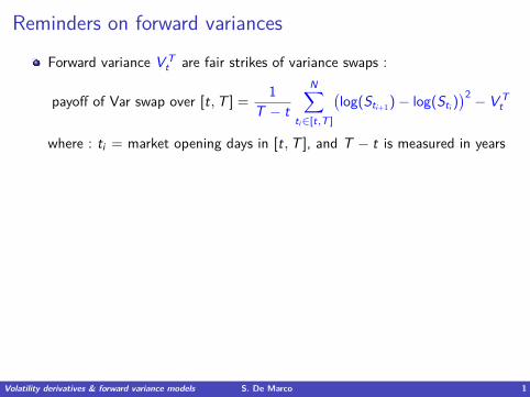
Forward variance V Tt are fair strikes of variance swaps :
payoff of Var swap over [t,T ] = 1T − t
N∑ti∈[t,T ]
(log(Sti+1 )− log(Sti )
)2 − V Tt
where : ti = market opening days in [t,T ], and T − t is measured in years
The value of V Tt is set so that
pricet(var swap) = 0.Take T2 > T1. By combining positions in var swaps over [t,T2] and [t,T1],we construct the payoff
1T2 − T1
∑ti∈[T1,T2]
(log(Sti+1 )− log(Sti )
)2 − V T1,T2t
whereV T1,T2
t = (T2 − t)V T2t − (T1 − t)V T1
tT2 − T1
is the forward variance over [T1,T2].
Volatility derivatives & forward variance models S. De Marco 1
Reminders on forward variances
Forward variance V Tt are fair strikes of variance swaps :
payoff of Var swap over [t,T ] = 1T − t
N∑ti∈[t,T ]
(log(Sti+1 )− log(Sti )
)2 − V Tt
where : ti = market opening days in [t,T ], and T − t is measured in yearsThe value of V T
t is set so thatpricet(var swap) = 0.
Take T2 > T1. By combining positions in var swaps over [t,T2] and [t,T1],we construct the payoff
1T2 − T1
∑ti∈[T1,T2]
(log(Sti+1 )− log(Sti )
)2 − V T1,T2t
whereV T1,T2
t = (T2 − t)V T2t − (T1 − t)V T1
tT2 − T1
is the forward variance over [T1,T2].
Volatility derivatives & forward variance models S. De Marco 1
Forward variances can be traded
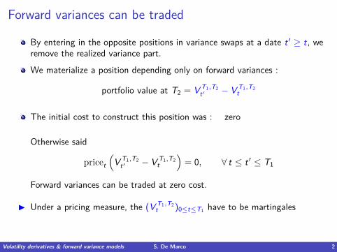
By entering in the opposite positions in variance swaps at a date t ′ ≥ t, weremove the realized variance part.
We materialize a position depending only on forward variances :
portfolio value at T2 = V T1,T2t′ − V T1,T2
t
The initial cost to construct this position was : zero
Otherwise said
pricet
(V T1,T2
t′ − V T1,T2t
)= 0, ∀ t ≤ t ′ ≤ T1
Forward variances can be traded at zero cost.
I Under a pricing measure, the (V T1,T2t )0≤t≤T1 have to be martingales
Volatility derivatives & forward variance models S. De Marco 2
Forward variances can be traded
By entering in the opposite positions in variance swaps at a date t ′ ≥ t, weremove the realized variance part.
We materialize a position depending only on forward variances :
portfolio value at T2 = V T1,T2t′ − V T1,T2
t
The initial cost to construct this position was : zero
Otherwise said
pricet
(V T1,T2
t′ − V T1,T2t
)= 0, ∀ t ≤ t ′ ≤ T1
Forward variances can be traded at zero cost.
I Under a pricing measure, the (V T1,T2t )0≤t≤T1 have to be martingales
Volatility derivatives & forward variance models S. De Marco 2
Instantaneous forward variance ξTt
Define instantaneous forward variance by
ξTt = d
dT((T − t)V T
t), t < T
so thatV T
t = 1T − t
∫ T
tξu
t du, t < T
andV T1,T2
t = 1T2 − T1
∫ T2
T1
ξut du, t < T1 < T2.
Note that if ∆ is small, then
V T ,T +∆t ≈ ξT
t
Volatility derivatives & forward variance models S. De Marco 3
A class of models based on Gaussian processes
ξTt = ξT
0 exp(∫ t
0K (T − s) · dWs −
12
∫ t
0K (T − s) · ρK (T − s)ds
)t ≤ T
I (ξT0 )T≥0 is the initial forward variance curve – a market parameter.
I W is a Brownian motion in Rn with correlation matrix ρ, and∫ t
0K (T − s) · dWs =
n∑i=1
∫ t
0Ki (T − s)dW i
s∫ t
0K (T − s) · ρK (T − s)ds =
n∑i,j=1
∫ t
0Ki (T − s)ρi,jKj(T − s)ds
I Deterministic kernels Ki ∈ L2loc(R+,R∗+).
Volatility derivatives & forward variance models S. De Marco 4
A class of models based on Gaussian processes
ξTt = ξT
0 exp(∫ t
0K (T − s) · dWs −
12
∫ t
0K (T − s) · ρK (T − s)ds
)t ≤ T
For every T , (ξTt )t≤T is the solution of the SDE
ξTt = ξT
t K (T − t) · dWt , t ≤ T
Does not belong to the affine family.
Interest for simulation/calibration : only Gaussian r.v. are involved.
Choice of kernels in practice : τ 7→ K (τ) decreasing.
Volatility derivatives & forward variance models S. De Marco 5
Parametric examples (I)
Bergomi’s model [Bergomi 05], [Dupire 93] with n = 1 factorK (τ) = ω e−kτ
with ω, k > 0.
ξTt = ξT
0 E(ω
∫ t
0e−k(T−s)dWs
)= ξT
0 E(ω e−k(T−t)
∫ t
0e−k(t−s)dWs
)= ξT
0 exp(
K (T − t)Xt −12
∫ t
0K (T − s)2ds
)where X is the OU process dXt = −k Xt + dWt .
I For every t, ξTt = Φ(T − t,Xt) : the forward variance curve ξT
· is a functionof one single Markov factor X .
Bergomi’s n-factor model [Bergomi 05] is the n-dim extension :Ki (τ) = ωi e−kiτ
Volatility derivatives & forward variance models S. De Marco 6
Parametric examples (I)
Bergomi’s model [Bergomi 05], [Dupire 93] with n = 1 factorK (τ) = ω e−kτ
with ω, k > 0.
ξTt = ξT
0 E(ω
∫ t
0e−k(T−s)dWs
)= ξT
0 E(ω e−k(T−t)
∫ t
0e−k(t−s)dWs
)= ξT
0 exp(
K (T − t)Xt −12
∫ t
0K (T − s)2ds
)where X is the OU process dXt = −k Xt + dWt .
I For every t, ξTt = Φ(T − t,Xt) : the forward variance curve ξT
· is a functionof one single Markov factor X .Bergomi’s n-factor model [Bergomi 05] is the n-dim extension :
Ki (τ) = ωi e−kiτ
Volatility derivatives & forward variance models S. De Marco 6
Parametric examples (II)
The rough Bergomi model of [Bayer, Friz, Gatheral 2016] :
K (τ) = ω
τ12−H
, H ∈ (0, 1/2)
so that
ξTt = ξT
0 exp(ω
∫ t
0
1(T − s) 1
2−HdWs −
12ω
2∫ t
0
1(T − s)1−2H ds
)
I Do not have a low-dimensional Markovian representation of the curve
T 7→ (ξTt )T≥t
For the moment (in this presentation), nothing in this model is rough.
For every T , the processes
(ξTt )t≤T are martingales
Volatility derivatives & forward variance models S. De Marco 7
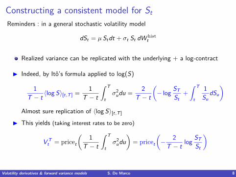
Constructing a consistent model for StReminders : in a general stochastic volatility model
dSt = µStdt + σt St dW histt
Realized variance can be replicated with the underlying + a log-contract
I Indeed, by Ito’s formula applied to log(S)
1T − t 〈log S〉[t,T ] = 1
T − t
∫ T
tσ2
udu = 2T − t
(− log ST
St+∫ T
t
1Su
dSu
)Almost sure replication of 〈log S〉[t,T ]
I This yields (taking interest rates to be zero)
V Tt = pricet
(1
T − t
∫ T
tσ2
udu)
= pricet
(− 2
T − t log STSt
)
Volatility derivatives & forward variance models S. De Marco 8
A consistent model for StGiven instantaneous forward variances ξT
t
The modeldSt = St
√ξt
t dZt
where Z is a Brownian motion, is consistent with the given ξTt
In the sense : the price of the log-contract in this model is
pricet
(−2
T − t log STSt
)= E
[1
T − t
∫ T
tξu
u du∣∣∣Ft
]= 1
T − t
∫ T
tE [ξu
u |Ft ]du = 1T − t
∫ T
tξu
t du
where Ft = FW ,Zt
I Hedging of European options on S with underlying + forward variances
Volatility derivatives & forward variance models S. De Marco 9
Rough Bergomi model, again
To see what is rough in rough Bergomi
we have to look at the consistent model for S :
dSt = St√ξt
t dZt
The instantaneous volatility ξtt of S is rough because
ξtt = exp
(ω x t
t −12ω
2∫ t
0
1(t − s)1−2H ds
)and
x tt =
∫ t
0
1(t − s) 1
2−HdWs
is a Volterra process which admits a β-Holder modification for β < H
Volatility derivatives & forward variance models S. De Marco 10
The VIX index
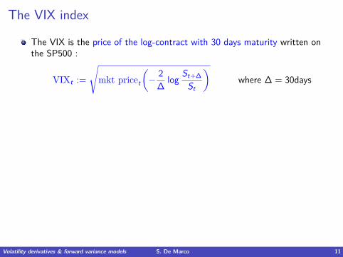
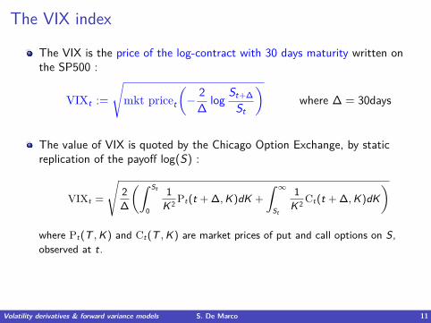
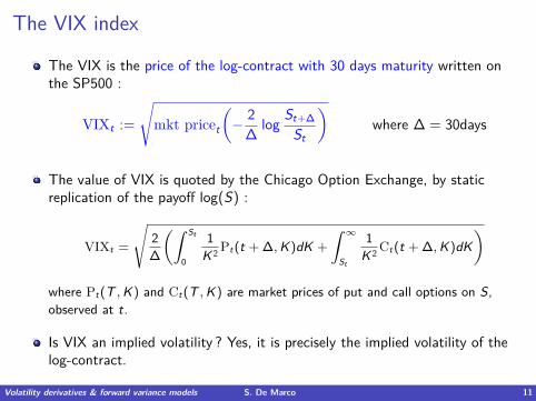
The VIX is the price of the log-contract with 30 days maturity written onthe SP500 :
VIXt :=
√mkt pricet
(− 2
∆ log St+∆St
)where ∆ = 30days
The value of VIX is quoted by the Chicago Option Exchange, by staticreplication of the payoff log(S) :
VIXt =
√2∆
(∫ St
0
1K 2 Pt(t + ∆,K)dK +
∫ ∞St
1K 2 Ct(t + ∆,K)dK
)where Pt(T ,K) and Ct(T ,K) are market prices of put and call options on S,observed at t.
Is VIX an implied volatility ? Yes, it is precisely the implied volatility of thelog-contract.
Volatility derivatives & forward variance models S. De Marco 11
The VIX index
The VIX is the price of the log-contract with 30 days maturity written onthe SP500 :
VIXt :=
√mkt pricet
(− 2
∆ log St+∆St
)where ∆ = 30days
The value of VIX is quoted by the Chicago Option Exchange, by staticreplication of the payoff log(S) :
VIXt =
√2∆
(∫ St
0
1K 2 Pt(t + ∆,K)dK +
∫ ∞St
1K 2 Ct(t + ∆,K)dK
)where Pt(T ,K) and Ct(T ,K) are market prices of put and call options on S,observed at t.
Is VIX an implied volatility ?
Yes, it is precisely the implied volatility of thelog-contract.
Volatility derivatives & forward variance models S. De Marco 11
The VIX index
The VIX is the price of the log-contract with 30 days maturity written onthe SP500 :
VIXt :=
√mkt pricet
(− 2
∆ log St+∆St
)where ∆ = 30days
The value of VIX is quoted by the Chicago Option Exchange, by staticreplication of the payoff log(S) :
VIXt =
√2∆
(∫ St
0
1K 2 Pt(t + ∆,K)dK +
∫ ∞St
1K 2 Ct(t + ∆,K)dK
)where Pt(T ,K) and Ct(T ,K) are market prices of put and call options on S,observed at t.
Is VIX an implied volatility ? Yes, it is precisely the implied volatility of thelog-contract.
Volatility derivatives & forward variance models S. De Marco 11
History of VIX (2006-2011)
Volatility derivatives & forward variance models S. De Marco 12
VIX in a stochastic volatility model
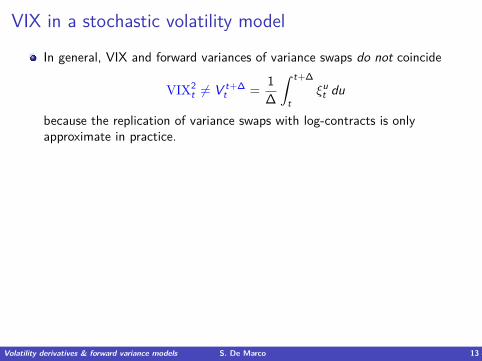
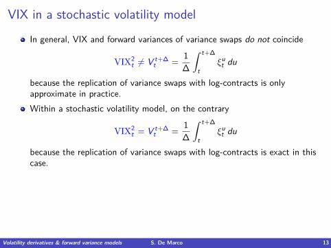
In general, VIX and forward variances of variance swaps do not coincide
VIX2t 6= V t+∆
t = 1∆
∫ t+∆
tξu
t du
because the replication of variance swaps with log-contracts is onlyapproximate in practice.
Within a stochastic volatility model, on the contrary
VIX2t = V t+∆
t = 1∆
∫ t+∆
tξu
t du
because the replication of variance swaps with log-contracts is exact in thiscase.Consequence : in general, we will be able to calibrate a forward variancemodel (St , ξ
·t) to at most 2 of the 3 different markets :
I VIX marketI SP500 options marketI Variance swap market on SP500
Volatility derivatives & forward variance models S. De Marco 13
VIX in a stochastic volatility model
In general, VIX and forward variances of variance swaps do not coincide
VIX2t 6= V t+∆
t = 1∆
∫ t+∆
tξu
t du
because the replication of variance swaps with log-contracts is onlyapproximate in practice.Within a stochastic volatility model, on the contrary
VIX2t = V t+∆
t = 1∆
∫ t+∆
tξu
t du
because the replication of variance swaps with log-contracts is exact in thiscase.
Consequence : in general, we will be able to calibrate a forward variancemodel (St , ξ
·t) to at most 2 of the 3 different markets :
I VIX marketI SP500 options marketI Variance swap market on SP500
Volatility derivatives & forward variance models S. De Marco 13
VIX in a stochastic volatility model
In general, VIX and forward variances of variance swaps do not coincide
VIX2t 6= V t+∆
t = 1∆
∫ t+∆
tξu
t du
because the replication of variance swaps with log-contracts is onlyapproximate in practice.Within a stochastic volatility model, on the contrary
VIX2t = V t+∆
t = 1∆
∫ t+∆
tξu
t du
because the replication of variance swaps with log-contracts is exact in thiscase.Consequence : in general, we will be able to calibrate a forward variancemodel (St , ξ
·t) to at most 2 of the 3 different markets :
I VIX marketI SP500 options marketI Variance swap market on SP500
Volatility derivatives & forward variance models S. De Marco 13
Pricing of VIX derivatives at t = 0The price at t = 0 of a VIX option with payoff ϕ is
E [ϕ(VIXT)] = E[ϕ
(√V T +∆
T
)]= Ψ(0, ξ·0)
where
Ψ(0, x ·) = E
[ϕ
((1∆
∫ T +∆
Txu e
∫ T
0K(u−s)·dWs − 1
2 h(0,T ,u)du)1/2)]
and h(t,T , u) =∫ T
t K (u − s) · ρK (u − s)ds.
If Markov repr (e.g. classical Bergomi),∫ T
0 K (u − s) · dWs = K (u − T ) XT
Otherwise : finite point (ui )i=1,...,N quadrature formula + simulation of thecorrelated Gaussian vector(∫ T
0K (u1, s) · dWs , . . . ,
∫ T
0K (uN , s) · dWs
); see A. Jacquier’s talk for rates of convergence.
Volatility derivatives & forward variance models S. De Marco 14
Term structure of volatility of volatilityI Denote
σ(t,T )
the at-the-money implied volatility of an option on the forward volatility√
V Tt .
Proposition (ATM implied volatility of forward volatility)The following asymptotics hold : for every T
σ(t,T ) −→t→0
σ(0,T ) := 12∫ T
0 ξu0 du
√∫ T
0ξu
0 K (u) · ρ∫ T
0ξu′
0 K (u′)du′
By choosing the kernels K , we can reach a prescribed target behavior ofσ(0,T )
Volatility derivatives & forward variance models S. De Marco 15
Term structure of volatility of volatility
I Black dots : target behavior for σ(0,T ), as a function of T (months).
I Very well described by a power law 1T α , α ≈ 0.4− 0.5
Volatility derivatives & forward variance models S. De Marco 16
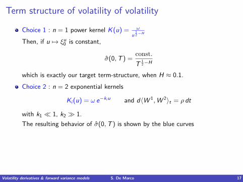
Term structure of volatility of volatility
Choice 1 : n = 1 power kernel K (u) = ω
u12−H
Then, if u 7→ ξu0 is constant,
σ(0,T ) = const.T 1
2−H
which is exactly our target term-structure, when H ≈ 0.1.
Choice 2 : n = 2 exponential kernels
Ki (u) = ω e−ki u and d〈W 1,W 2〉t = ρ dt
with k1 � 1, k2 � 1.The resulting behavior of σ(0,T ) is shown by the blue curves
I A model with fractional kernel reaches the target behavior with n = 1 factorand two parameters ω,H.
I A classical Bergomi model does this with n = 2 factors and four parametersk1, k2, ρ, ω.
Volatility derivatives & forward variance models S. De Marco 17
An extended class of forward variance modelsAs mentioned by Antoine, in the class of models above
The ξTt are log-normal. Forward variances 1
∆∫ T +∆
T ξuT du are close to
log-normal.
Incapability of generate a reasonable smile for VIX options.
I Inspired by [Bergomi 2008], we set
ξTt = ξT
0 f T (t, xTt )
where xTt denotes our Gaussian factor
xTt =
∫ t
0K (T − s) · dWs
and the f T (·, ·) are smooth functions to be determined.
Volatility derivatives & forward variance models S. De Marco 18
An extended class of forward variance models
I We need to impose some conditions on f T :
f T (t, x) ≥ 0
Initial condition ξT0 ⇒ = f T (0, 0) = 1, ∀T
(ξTt )0≤t≤T needs to be martingale :
dξTt =
(∂t f T (t, xT
t ) + 12K · ρK ∂xx f T (t, xT
t ))
dt + ∂x f T (t, xTt )dxT
t
Therefore, we require that the f T (·) solve the family of PDE
∂t f T (t, x) + 12K (T − t) · ρK (T − t)∂xx f (t, x) = 0, ∀(t, x) ∈ [0,T ]×R.
Volatility derivatives & forward variance models S. De Marco 19
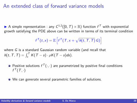
An extended class of forward variance models
I A simple representation : any C1,2([0,T )× R) function f T with exponentialgrowth satisfying the PDE above can be written in terms of its terminal condition
f T (t, x) = E[f T (T , x +
√h(t,T ,T ) G)
]where G is a standard Gaussian random variable (and recall thath(t,T ,T ) =
∫ Tt K (T − s) · ρK (T − s)ds).
Positive solutions f T (·, ·) are parametrized by positive final conditionsf T (T , ·)
We can generate several parametric families of solutions.
Volatility derivatives & forward variance models S. De Marco 20
Parametric choice 1 : polynomials
The terminal condition :f T (T , y) = a(T )y2 + b(T )y + c(T )
leads to a quadratic Gaussian model
ξTt = ξT
0 f T (t, xTt ) = ξT
0
(a(T )
[(xT
t )2 − h(t,T )]
+ b(T )xTt + 1
)where h(t,T ) =
∫ t0 K (T − s) · ρK (T − s)ds
I We are free to choose a(T ), b(T ) s.t. 1− a(T )h(T ,T )− b(T )2
t has a χ2 distribution.The more general terminal condition :
f T (T , y) =n∑
k=0aT
k y2k
leads to polynomial functions x 7→ f T (t, x).Volatility derivatives & forward variance models S. De Marco 21
Parametric choice 2 : exponentials
The terminal condition :
f T (T , y) =m∑
k=1γk e ωk y where
m∑k=1
γk = 1, m ∈ N
leads to a linear combination of Laplace transforms of a Gaussian r.v.
f T (t, x) =m∑
k=1γk e ωk x − 1
2 (ωk )2h(t,T )
I The class of models we started from corresponds to m = 1.
With this choice, forward variancesξT
t = f T (t, xTt )
are sums of log-normals which can be made very different from a singlelog-normalWe have expressions and numerical methods for VIX derivatives similar tothe previous case (where m = 1).
Volatility derivatives & forward variance models S. De Marco 22
A simple version of the rough model where forwardvariances are not log-normalRough model (n = 1,m = 2) : n = 1 gaussian factor, and m = 2 basis functions
f T (t, x) = (1− γT ) exp(ωT
1 x−12 (ωT
1 )2h(t,T ))
+ γT exp(ωT
2 x−12 (ωT
2 )2h(t,T ))
ξTt = ξT
0 f T (t, xTt )
xTt =
∫ t
0K (T − s)dWs , K (T − s) = 1
(T − s) 12−H
I This model depends on the global parameter
H
and on the four term-structure parameters
ξT0 , γ
T , ωT1 , ω
T2
which we can use to fit an initial term-structure of VIX Futures and the smiles ofVIX options.
Volatility derivatives & forward variance models S. De Marco 23
Calibration to VIX market (m = 2 exponential fcts)
VIX Futures (left) and VIX implied volatilities (right) on 22 Nov 2017, T = 20 Dec