S Evaluation Language Modelling for R - MIT OpenCourseWare · PDF fileLanguage Model R...

Language Modelling for Speech Recognition

• Introduction

• n-gram language models

• Probability estimation

• Evaluation

• Beyond n-grams

6.345 Automatic Speech Recognition Language Modelling 1

rahkuma

Lecture # 11-12 Session 2003

�

Language Modelling for Speech Recognition

ˆ • Speech recognizers seek the word sequence W which is most likely to be produced from acoustic evidence A

P(W |A) = max P(W |A) ∝ max P(A|W )P(W ) W W

• Speech recognition involves acoustic processing, acoustic modelling, language modelling, and search

• Language models (LMs) assign a probability estimate P(W ) to word sequences W = {w1, . . . , wn} subject to

P(W ) = 1 W

• Language models help guide and constrain the search among alternative word hypotheses during recognition


Language Model Requirements

�

Coverage

� Constraint

�

Understanding

NLP

�

�

�


Finite-State Networks (FSN)

show me all the flights

give restaurants

display

• Language space defined by a word network or graph

• Describable by a regular phrase structure grammar

A =⇒ aB | a

• Finite coverage can present difficulties for ASR

• Graph arcs or rules can be augmented with probabilities


Context-Free Grammars (CFGs)

VP

NP

V D N

display the flights

• Language space defined by context-free rewrite rules

e.g., A =⇒ BC | a

• More powerful representation than FSNs

• Stochastic CFG rules have associated probabilities which can be learned automatically from a corpus

• Finite coverage can present difficulties for ASR6.345 Automatic Speech Recognition Language Modelling 5

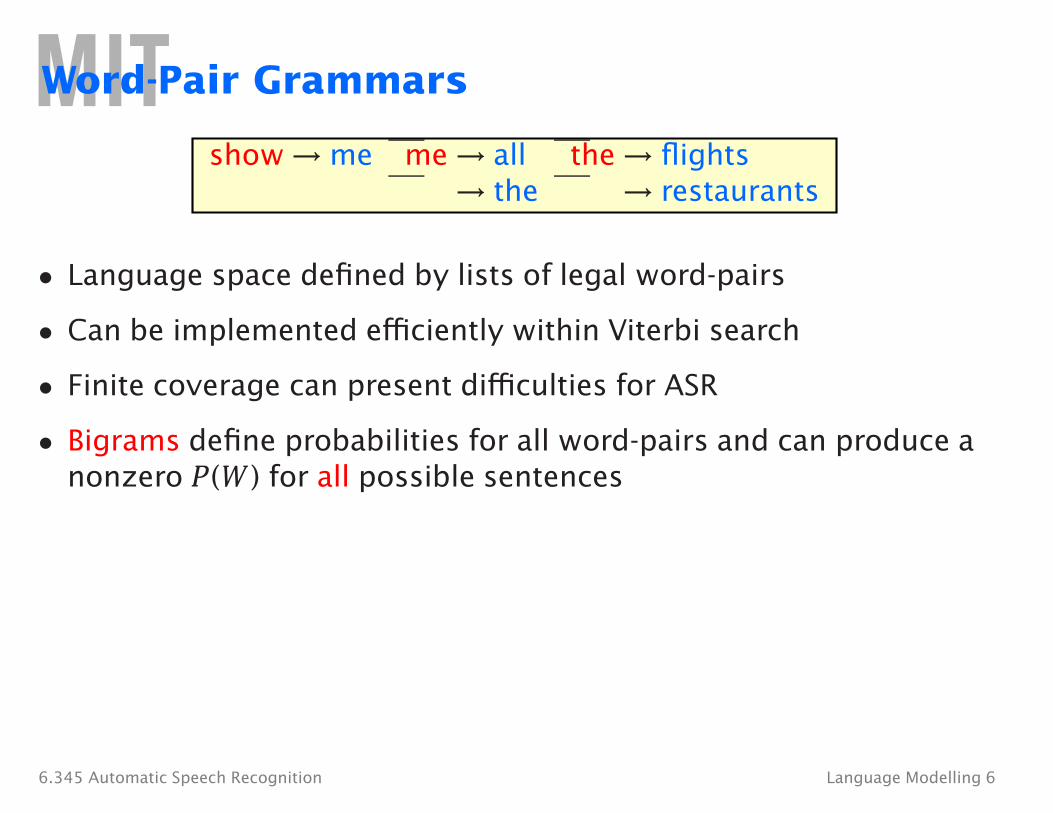
Word-Pair Grammars

show → me me → all the → flights → the → restaurants

• Language space defined by lists of legal word-pairs

• Can be implemented efficiently within Viterbi search

• Finite coverage can present difficulties for ASR

• Bigrams define probabilities for all word-pairs and can produce a nonzero P(W ) for all possible sentences


Example of LM Impact (Lee, 1988)

• Resource Management domain

• Speaker-independent, continuous-speech corpus

• Sentences generated from a finite state network

• 997 word vocabulary

• Word-pair perplexity ∼ 60, Bigram ∼ 20

• Error includes substitutions, deletions, and insertions

No LM Word-Pair Bigram % Word Error Rate 29.4 6.3 4.2


� ) =

�

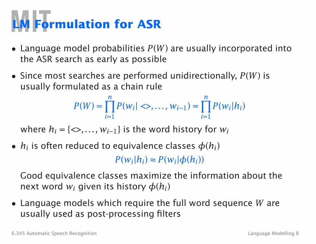
LM Formulation for ASR

• Language model probabilities P(W ) are usually incorporated into the ASR search as early as possible

• Since most searches are performed unidirectionally, P(W ) is usually formulated as a chain rule

P(W ) = n

i=1

P(wi | <>, . . . , wi−1

n

i=1

P(wi |hi )

where hi = {<>, . . . , wi−1} is the word history for wi

• hi is often reduced to equivalence classes φ(hi )

P(wi |hi ) ≈ P(wi |φ(hi ))

Good equivalence classes maximize the information about the next word wi given its history φ(hi )

• Language models which require the full word sequence W are usually used as post-processing filters


1 2 3

1 2

�

n-gram Language Models

• n-gram models use the previous n − 1 words to represent the history φ(hi ) = {wi−1 , . . . , wi−(n−1)}

• Probabilities are based on frequencies and counts

c(w w w ) e.g., f (w 3|w 1 w 2) =

c(w w )

• Due to sparse data problems, n-grams are typically smoothed with lower order frequencies subject to

P(w|φ(hi )) = 1 w

• Bigrams are easily incorporated in Viterbi search

• Trigrams used for large vocabulary recognition in mid-1970’s and remain the dominant language model


123456789

IBM Trigram Example (Jelinek, 1997)

The are to know the issues This will have this problems One the understand these the Two would doA also getThree do thePlease need useIn provideWe insert

• •• •

96 write 97 me 98 resolve

••

163916401641

problemsanyaproblemthemall

necessarydatainformationaboveothertimepeopleoperatorstools••jobs MVS old ••reception shop important


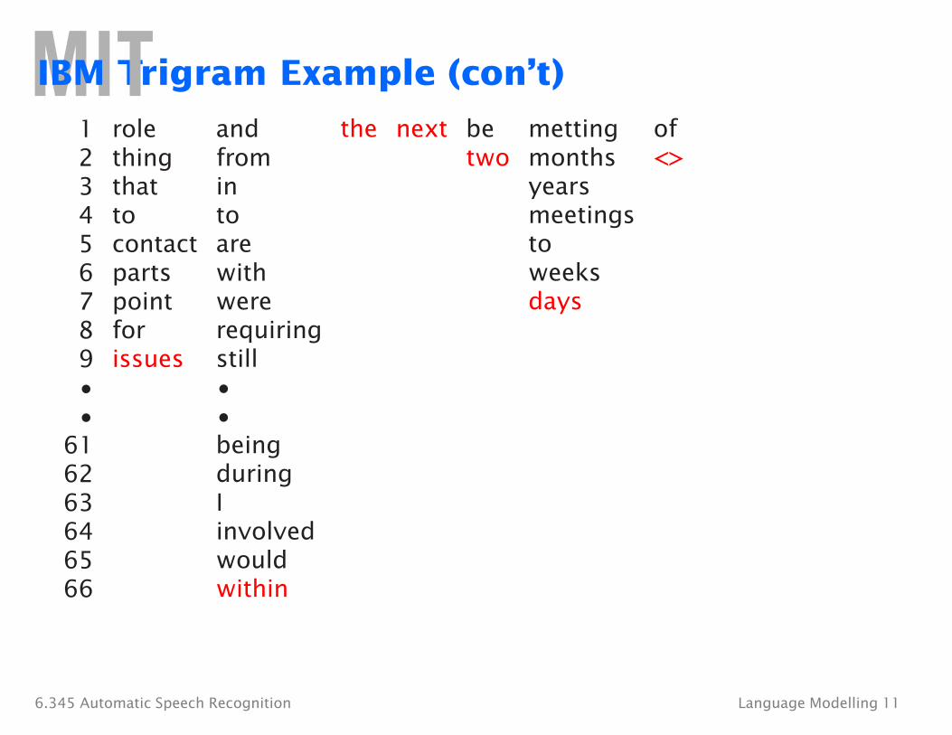
123456789

IBM Trigram Example (con’t)

••

61 62 63 64 65 66

rolethingthattocontactpartspointforissues

and the next befrom twointoarewithwererequiringstill••beingduringIinvolvedwouldwithin

metting ofmonths <>yearsmeetingstoweeksdays


n

n-gram Issues: Sparse Data (Jelinek, 1985)

• Text corpus of IBM patent descriptions

• 1.5 million words for training

• 300,000 words used to test models

• Vocabulary restricted to 1,000 most frequent words

• 23% of trigrams occurring in test corpus were absent from training corpus!

• In general, a vocabulary of size V will have V n-grams (e.g., 20,000 words will have 400 million bigrams, and 8 trillion trigrams!)


�

j

λ j �

j

λ j

V

n-gram Interpolation

• Probabilities are a linear combination of frequencies

P(wi |hi ) = f (wi |φj (hi )) = 1

1e.g., P(w2|w1) = λ2f (w2|w1) + λ1f (w2) + λ0

• λ’s computed with EM algorithm on held-out data

• Different λ’s can be used for different histories hi

c(w1)c(w1) + k

• Simplistic formulation of λ’s can be used λ =

• Estimates can be solved recursively:

P(w3|w1w2) = λ3f (w3|w1w2) + (1 − λ3)P(w3|w2)

P(w3|w2) = λ2f (w3|w2) + (1 − λ2)P(w3)


V

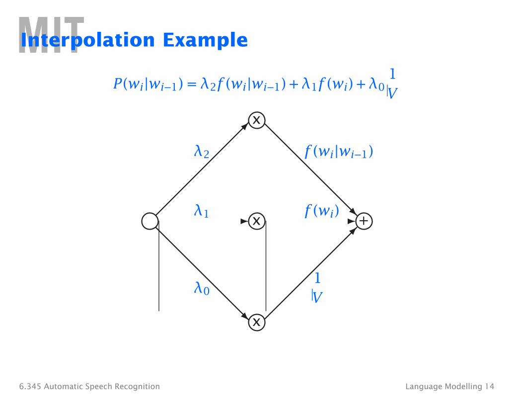
Interpolation Example

1P(wi |wi−1) = λ2f (wi |wi−1) + λ1f (wi ) + λ0

�

�

�

�

�

� x

x

x

+

λ2

λ1

λ0 1 V

f (w i )

f (w i |w i−1)


j �

j n i i

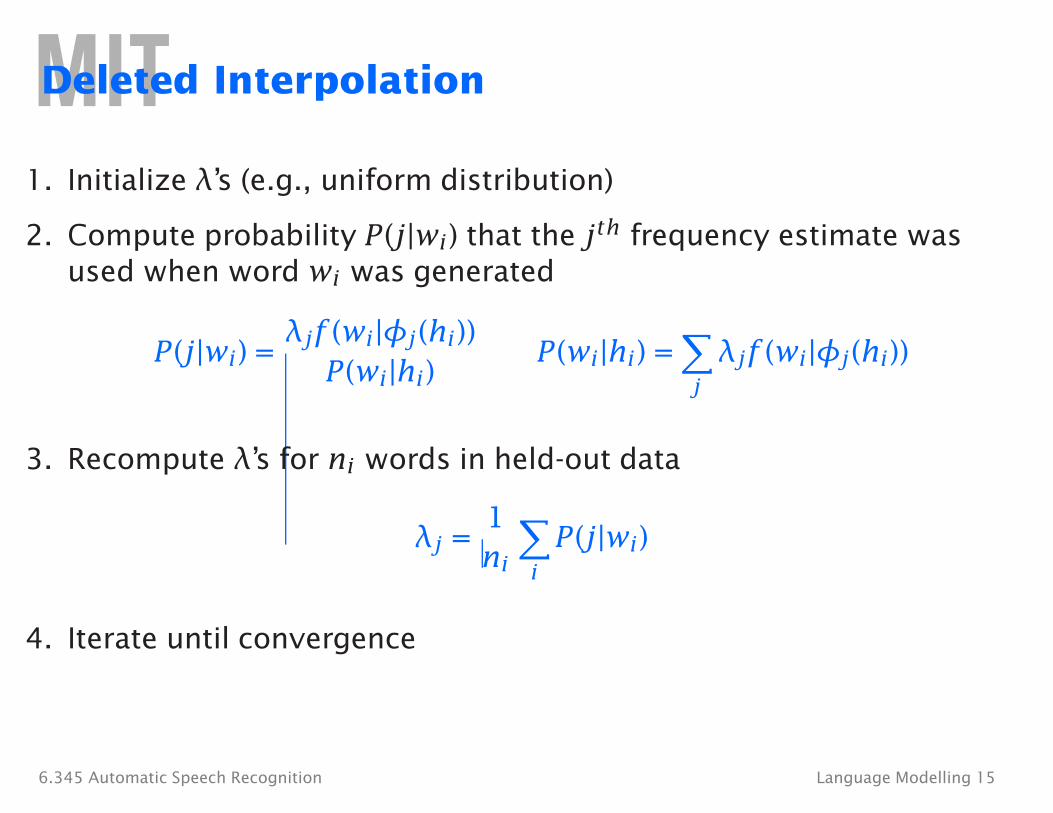
Deleted Interpolation

1. Initialize λ’s (e.g., uniform distribution)

2. Compute probability P(j|wi ) that the jth frequency estimate was used when word wi was generated

λ f (wi |φj (hi )) P(wi |hi ) = λjf (wi |φj (hi ))P(j|wi ) =

P(wi |hi ) j

3. Recompute λ’s for ni words in held-out data

1 � λ = P(j|wi )

4. Iterate until convergence


�

w

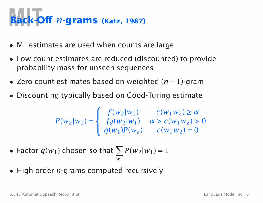
Back-Off n-grams (Katz, 1987)

• ML estimates are used when counts are large

• Low count estimates are reduced (discounted) to provide probability mass for unseen sequences

• Zero count estimates based on weighted (n − 1)-gram

• Discounting typically based on Good-Turing estimate f (w2|w1) c(w1w2) ≥ α P(w2|w1) = fd (w2|w1) α > c(w1w2) > 0 q(w1)P(w2) c(w1w2) = 0

• Factor q(w1) chosen so that P(w2|w1) = 1 2

• High order n-grams computed recursively


N

� N r

�

n N

n N

r r N

n n r

Good-Turing Estimate

• Probability a word will occur r times out of N , given θ

p (r|θ) = θr (1 − θ)N−r

• Probability a word will occur r + 1 times out of N + 1

N + 1 pN+1(r + 1|θ) =

r + 1 θpN (r|θ)

• Assume nr words occuring r times have same value of θ

r r+1 pN (r|θ) ≈ pN+1(r + 1|θ) ≈

∗ • Assuming large N , we can solve for θ or discounted r ∗ ∗ r+1

θ = P = r = (r + 1)


P r r N

r n n r

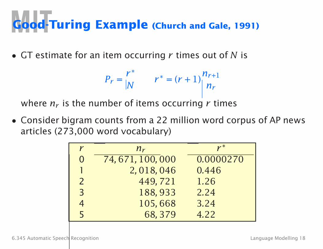
Good-Turing Example (Church and Gale, 1991)

• GT estimate for an item occurring r times out of N is

∗ ∗ r+1= (r + 1)=

where nr is the number of items occurring r times

• Consider bigram counts from a 22 million word corpus of AP news articles (273,000 word vocabulary)

r n r r ∗

0 1 2 3 4 5

74, 671, 100, 000 2, 018, 046

449, 721 188, 933 105, 668 68, 379

0.0000270 0.446 1.26 2.24 3.24 4.22


Integration into Viterbi Search

Preceding Following Words Words

Bigrams can be efficiently incorporated into Viterbi search using an intermediate node between words

• Interpolated: Q (wi ) = (1 − λi )

• Back-off: Q (wi ) = q(wi )


P(wj)

P(wj|wi)

Q(wi)

Evaluating Language Models

• Recognition accuracy

• Qualitative assessment

– Random sentence generation

– Sentence reordering

• Information-theoretic measures


Random Sentence Generation: Air Travel Domain Bigram

Show me the flight earliest flight from DenverHow many flights that flight leaves around is the Eastern DenverI want a first classShow me a reservation the last flight from Baltimore for the firstI would like to fly from DallasI get from PittsburghWhich just smallIn Denver on OctoberI would like to San FranciscoIs flight flyingWhat flights from Boston to San FranciscoHow long can you book a hundred dollarsI would like to Denver to Boston and BostonMake ground transportation is the cheapestAre the next week on AA eleven tenFirst classHow many airlines from Boston on May thirtiethWhat is the city of three PMWhat about twelve and Baltimore


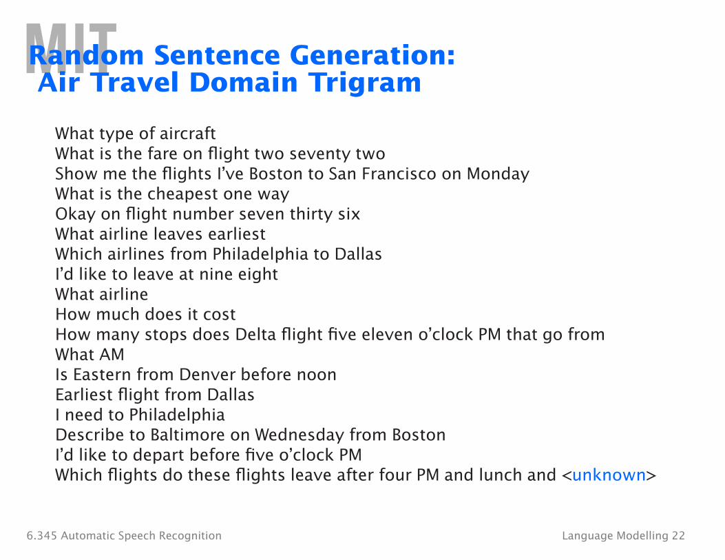
Random Sentence Generation: Air Travel Domain Trigram

What type of aircraftWhat is the fare on flight two seventy twoShow me the flights I’ve Boston to San Francisco on MondayWhat is the cheapest one wayOkay on flight number seven thirty sixWhat airline leaves earliestWhich airlines from Philadelphia to DallasI’d like to leave at nine eightWhat airlineHow much does it costHow many stops does Delta flight five eleven o’clock PM that go fromWhat AMIs Eastern from Denver before noonEarliest flight from DallasI need to PhiladelphiaDescribe to Baltimore on Wednesday from BostonI’d like to depart before five o’clock PMWhich flights do these flights leave after four PM and lunch and <unknown>


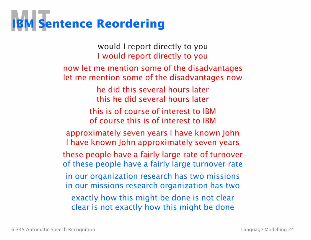
Sentence Reordering (Jelinek, 1991)

• Scramble words of a sentence

• Find most probable order with language model

• Results with trigram LM

– Short sentences from spontaneous dictation

– 63% of reordered sentences identical

– 86% have same meaning


IBM Sentence Reordering

would I report directly to you I would report directly to you

now let me mention some of the disadvantages let me mention some of the disadvantages now

he did this several hours later this he did several hours later

this is of course of interest to IBM of course this is of interest to IBM

approximately seven years I have known John I have known John approximately seven years

these people have a fairly large rate of turnover of these people have a fairly large turnover rate

in our organization research has two missions in our missions research organization has two

exactly how this might be done is not clear clear is not exactly how this might be done


Quantifying LM Complexity

• One LM is better than another if it can predict an n word test corpus W with a higher probability P(W )

• For LMs representable by the chain rule, comparisons are usually based on the average per word logprob, LP

1 ˆ 1 � ˆLP = − log2 P(W ) = − log2 P(wi |φ(hi ))

n n i

• A more intuitive representation of LP is the perplexity

PP = 2LP

(a uniform LM will have PP equal to vocabulary size)

• PP is often interpreted as an average branching factor


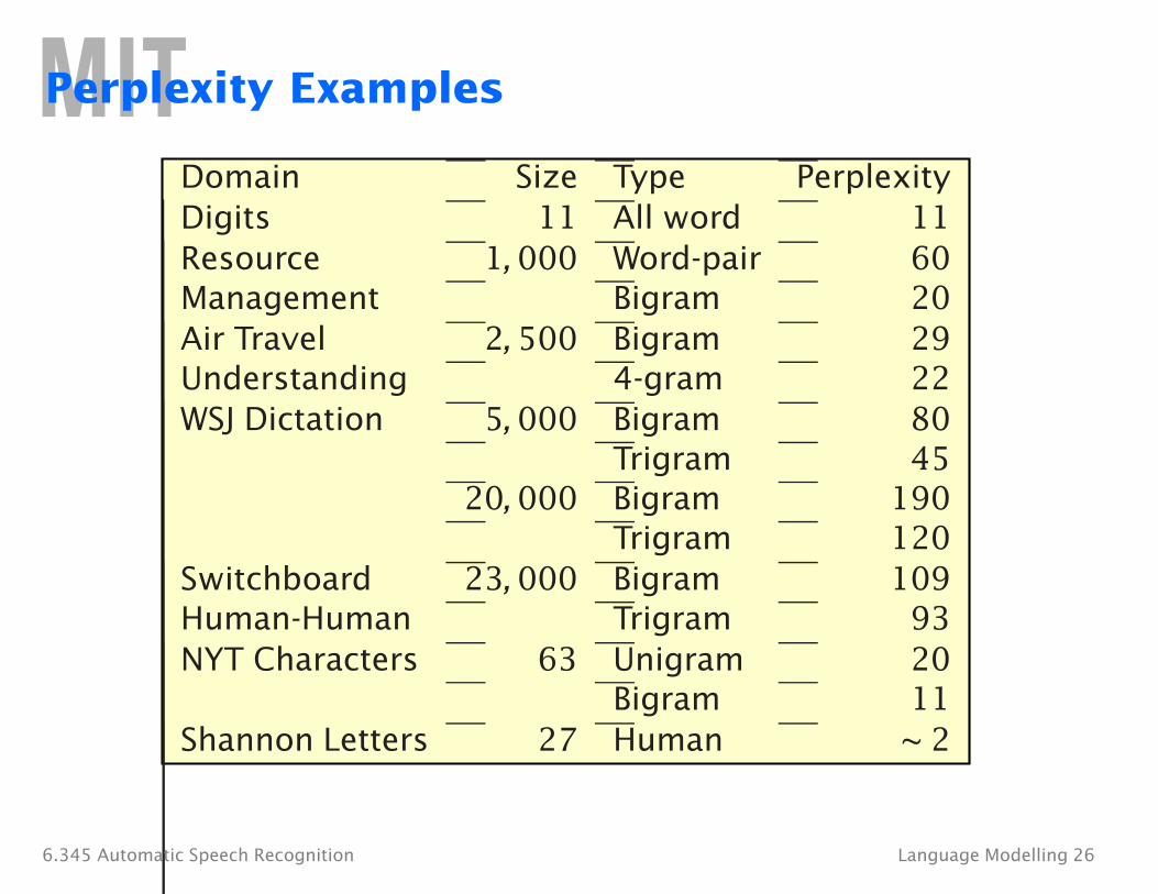
Perplexity Examples

Domain Size Type Perplexity Digits 11 All word 11 Resource 1, 000 Word-pair 60 Management Bigram 20 Air Travel 2, 500 Bigram 29 Understanding 4-gram 22 WSJ Dictation 5, 000 Bigram 80

Trigram 45 20, 000 Bigram 190

Trigram 120 Switchboard 23, 000 Bigram 109 Human-Human Trigram 93 NYT Characters 63 Unigram 20

Bigram 11 Shannon Letters 27 Human ∼ 2


Language Entropy

• The average logprob LP is related to the overall uncertainty of the language, quantified by its entropy

1 � H = − lim P(W ) log2 P(W )

n→∞ n W

• If W is obtained from a well-behaved source (ergodic), P(W ) will converge to the expected value and H is

1 1 H = − lim log2 P(W ) ≈ − log2 P(W ) n >> 1

n→∞ n n

• The entropy H is a theoretical lower bound on LP

1 � 1 � ˆ− lim P(W ) log2 P(W ) ≤ − lim P(W ) log2 P(W )

n→∞ n n→∞ nW W


�

Human Language Entropy (Shannon, 1951)

• An attempt to estimate language entropy of humans

• Involved guessing next words in order to measure subjects probability distribution

• Letters were used to simplify experiments

T H E R E I S N O R E V E R S E 1 1 1 5 1 1 2 1 1 2 1 1 15 1 17 1 1 1 2

O N A M O T O R C Y C L E A . . . 1 3 2 1 2 2 7 1 1 1 1 4 1 1 1 1 1 3 . . .

ˆ ˆ ˆ ˆ 24 ˆ 6 ˆ 2• H = − P(i) log2 P(i) P(1) = 37 P(2) = 37 P(3) = 37

ˆ • Shannon estimated H ≈ 1 bit/letter


Why do n-grams work so well?

• Probabilities are based on data (the more the better)

• Parameters determined automatically from corpora

• Incorporate local syntax, semantics, and pragmatics

• Many languages have a strong tendency toward standard word order and are thus substantially local

• Relatively easy to integrate into forward search methods such as Viterbi (bigram) or A∗


Problems with n-grams

• Unable to incorporate long-distance constraints

• Not well suited for flexible word order languages

• Cannot easily accommodate

– New vocabulary items

– Alternative domains

– Dynamic changes (e.g., discourse)

• Not as good as humans at tasks of

– Identifying and correcting recognizer errors

– Predicting following words (or letters)

• Do not capture meaning for speech understanding


Clustering words

• Many words have similar statistical behavior

– e.g., days of the week, months, cities, etc.

• n-gram performance can be improved by clustering words

– Hard clustering puts a word into a single cluster

– Soft clustering allows a word to belong to multiple clusters

• Clusters can be created manually, or automatically

– Manually created clusters have worked well for small domains

– Automatic clusters have been created bottom-up or top-down


Bottom-Up Word Clustering (Brown et al., 1992)

• Word clusters can be created automatically by forming clusters in a stepwise-optimal or greedy fashion

• Bottom-up clusters created by considering impact on metric of merging words wa and wb to form new cluster wab

• Example metrics for a bigram language model:

– Minimum decrease in average mutual information

� I = P(wiwj ) log2

P(wj |wi )

i,j P(wj )

– Minimum increase in training set conditional entropy � H = − P(wiwj ) log2 P(wj |wi )

i,j


Example of Word Clustering

A A

_M

AF

TE

RN

OO

N

AM

ER

ICA

N

AN

AN

Y

AU

GU

ST

AV

AIL

AB

LE

BE

BO

OK

BO

ST

ON

CIT

Y

CLA

SS

CO

AC

H

CO

NT

INE

NT

AL

CO

ST

DA

Y

DE

LTA

DO

LLA

RS

DO

WN

TO

WN

EA

ST

ER

N

EC

ON

OM

Y

EIG

HT

EIG

HT

Y

EV

EN

ING

FA

RE

F

AR

ES

FIF

TE

EN

FIF

TY

FIR

ST

_CLA

SS

FIV

E FLY

FO

RT

Y

FO

UR

FR

IDA

Y

GE

T

GIV

E

GO

GR

OU

ND

HU

ND

RE

D

INF

OR

MA

TIO

N

IT

JULY

KN

OW

LEA

ST

MA

KE

MA

Y

ME

AL

ME

ALS

MO

ND

AY

MO

RN

ING

NIN

E

NIN

ET

Y

NO

NS

TO

P

NO

VE

MB

ER

O+

CLO

CK

OH

ON

E

ON

E_W

AY

P_M

PLA

NE

RE

TU

RN

RO

UN

D_T

RIP

SA

TU

RD

AY

SC

EN

AR

IO

SE

RV

ED

SE

RV

ICE

SE

VE

N

SE

VE

NT

Y

SIX

SIX

TY

ST

OP

OV

ER

SU

ND

AY

TA

KE

TE

LL

TH

ER

E

TH

IRT

Y

TH

IS

TH

RE

E

TH

UR

SD

AY

TIC

KE

T

TIM

E

TIM

ES

TR

AN

SP

OR

TA

TIO

N

TR

AV

EL

TU

ES

DA

Y

TW

EN

TY

TW

O

U_S

_AIR

UN

ITE

D

US

ED

W

ILL

ZE

RO

NIL

46

02

DA

LLA

S_F

OR

T_W

OR

TH

WE

DN

ES

DA

Y

WA

SH

ING

TO

N

FIN

D

AIR

CR

AF

T

AIR

PLA

NE

LOW

ES

T

CH

EA

PE

ST

TH

ES

E

TH

OS

E

WO

ULD

N

EE

D

OA

KLA

ND

B

ALT

IMO

RE

KIN

D

TY

PE

EA

RLI

ES

T

LAT

ES

T

WA

NT

MO

ST

SA

N_F

RA

NC

ISC

O

PIT

TS

BU

RG

H

DA

LLA

S

PH

ILA

DE

LPH

IA

AT

LAN

TA

DE

NV

ER


�

Word Class n-gram models

• Word class n-grams cluster words into equivalence classes

W = {w1, . . . , wn} → {c1, . . . , cn}

• If clusters are non-overlapping, P(W ) is approximated by

n

P(W ) ≈ P(wi |ci )P(ci | <>, . . . , ci−1) i=1

• Fewer parameters than word n-grams

• Relatively easy to add new words to existing clusters

• Can be linearly combined with word n-grams if desired


Predictive Clustering (Goodman, 2000)

• For word class n-grams : P(wi |hi ) ≈ P(wi |ci )P(ci |ci−1 . . .)

• Predictive clustering is exact: P(wi |hi ) = P(wi |hici )P(ci |hi )

• History, hi , can be clustered differently for the two terms

• This model can be larger than the n-gram , but has been shown to produce good results when combined with pruning


Phrase Class n-grams (PCNG) (McCandless, 1994)

• Probabilistic context-free rules parse phrases

W = {w1, . . . , wn} → {u1, . . . , um }

• n-gram produces probability of resulting units

• P(W ) is product of parsing and n-gram probabilities

P(W ) = Pr (W )Pn(U )

• Intermediate representation between word-based n-grams and stochastic context-free grammars

• Context-free rules can be learned automatically


�

PCNG Example

NT2 NT4

NT1 NT3 NT0 NT0

Please show me the cheapest flight from Boston to Denver

NT2 the NT3 from NT0 NT4


PCNG Experiments

• Air-Travel Information Service (ATIS) domain

• Spontaneous, spoken language understanding

• 21,000 train, 2,500 development, 2,500 test sentences

• 1,956 word vocabulary

Language Model # Rules # Params Perplexity Word Bigram 0 18430 21.87 + Compound Words 654 20539 20.23 + Word Classes 1440 16430 19.93 + Phrases 2165 16739 15.87

PCNG Trigram 2165 38232 14.53 PCNG 4-gram 2165 51012 14.40


Decision Tree Language Models (Bahl et al., 1989)

• Equivalence classes represented in a decision tree

– Branch nodes contain questions for history hi

– Leaf nodes contain equivalence classes

• Word n-gram formulation fits decision tree model

• Minimum entropy criterion used for construction

• Significant computation required to produce trees


�

�

Exponential Language Models

• P(wi |hi ) modelled as product of weighted features fj (wihi )

j

λjfj (wihi )1

P(wi |hi ) = Z(hi )

e

where λ’s are parameters, and Z(hi ) is a normalization factor

• Binary-valued features can express arbitrary relationships

e.g., fj (wihi ) = 1 wi = A & wi−1 = B 0 else

• When E(f (wh)) corresponds to empirical expected value, ML estimates for λ’s correspond to maximum entropy distribution

• ML solutions are iterative, and can be extremely slow

• Demonstrated perplexity and WER gains on large vocabulary tasks


Adaptive Language Models

• Cache-based language models incorporate statistics of recently used words with a static language model

P(wi |hi ) = λPc (wi |hi ) + (1 − λ)Ps (wi |hi )

• Trigger-based language models increase word probabilities when key words observed in history hi

– Self triggers provide significant information

– Information metrics used to find triggers

– Incorporated into maximum entropy formulation


Trigger Examples (Lau, 1994)

• Triggers determined automatically from WSJ corpus (37 million words) using average mutual information

• Top seven triggers per word used in language model

Word Triggers

stocks stocks index investors market dow average industrial

political political party presidential politics election president campaign

foreign currency dollar japanese domestic exchange japan trade

bonds bonds bond yield treasury municipal treasury’s yields


Language Model Pruning

• n-gram language models can get very large (e.g., 6B/n-gram )

• Simple techniques can reduce parameter size

– Prune n-grams with too few occurrences

– Prune n-grams that have small impact on model entropy

• Trigram count-based pruning example:

– Broadcast news transcription (e.g., TV, radio broadcasts)

– 25K vocabulary; 166M training words (∼ 1GB), 25K test words

Count Bigrams Trigrams States Arcs Size Perplexity 0 6.4M 35.1M 6.4M 48M 360MB 157.4 1 3.2M 11.4M 2.2M 17M 125MB 169.4 2 2.2M 6.3M 1.2M 10M 72MB 178.1 3 1.7M 4.4M 0.9M 7M 52MB 185.1 4 1.4M 3.4M 0.7M 5M 41MB 191.9


�

Entropy-based Pruning (Stolcke, 1998)

• Uses KL distance to prune n-grams with low impact on entropy

D(P � P �) = P(wi |hj )

P(wi |hj ) log P �(wi |hj )i,j

PP � − PPPP

= eD(P�P �) − 1

1. Select pruning threshold θ

2. Compute perplexity increase from pruning each n-gram

3. Remove n-grams below θ, and recompute backoff weights

• Example: resorting Broadcast News N -best lists with 4-grams

θ Bigrams Trigrams 4-grams Perplexity % WER 0 11.1M 14.9M 0 172.5 32.9 0 11.1M 14.9M 3.3M 163.0 32.6

10−9 7.8M 9.6M 1.9M 163.9 32.6 10−8 3.2M 3.7M 0.7M 172.3 32.6 10−7 0.8M 0.5M 0.1M 202.3 33.9


Perplexity vs. Error Rate (Rosenfeld et al., 1995)

• Switchboard human-human telephone conversations

• 2.1 million words for training, 10,000 words for testing

• 23,000 word vocabulary, bigram perplexity of 109

• Bigram-generated word-lattice search (10% word error)

Trigram Condition Perplexity % Word Error Trained on Train Set 92.8 49.5 Trained on Train & Test Set 30.4 38.7 Trained on Test Set 17.9 32.9 No Parameter Smoothing 3.2 31.0

Perfect Lattice 3.2 6.3 Other Lattice 3.2 44.5


References

• X. Huang, A. Acero, and H. -W. Hon, Spoken Language Processing, Prentice-Hall, 2001.

• K. Church & W. Gale, A Comparison of the Enhanced Good-Turing and Deleted Estimation Methods for Estimating Probabilities of English Bigrams, Computer Speech & Language, 1991.

• F. Jelinek, Statistical Methods for Speech Recognition, MIT Press, 1997.

• S. Katz, Estimation of Probabilities from Sparse Data for the Language Model Component of a Speech Recognizer. IEEE Trans. ASSP-35, 1987.

• K. F. Lee, The CMU SPHINX System, Ph.D. Thesis, CMU, 1988.

• R. Rosenfeld, Two Decades of Statistical Language Modeling: Where Do We Go from Here?, IEEE Proceedings, 88(8), 2000.

• C. Shannon, Prediction and Entropy of Printed English, BSTJ, 1951. 6.345 Automatic Speech Recognition Language Modelling 46

More References

• L. Bahl et al., A Tree-Based Statistical Language Model for Natural Language Speech Recognition, IEEE Trans. ASSP-37, 1989.

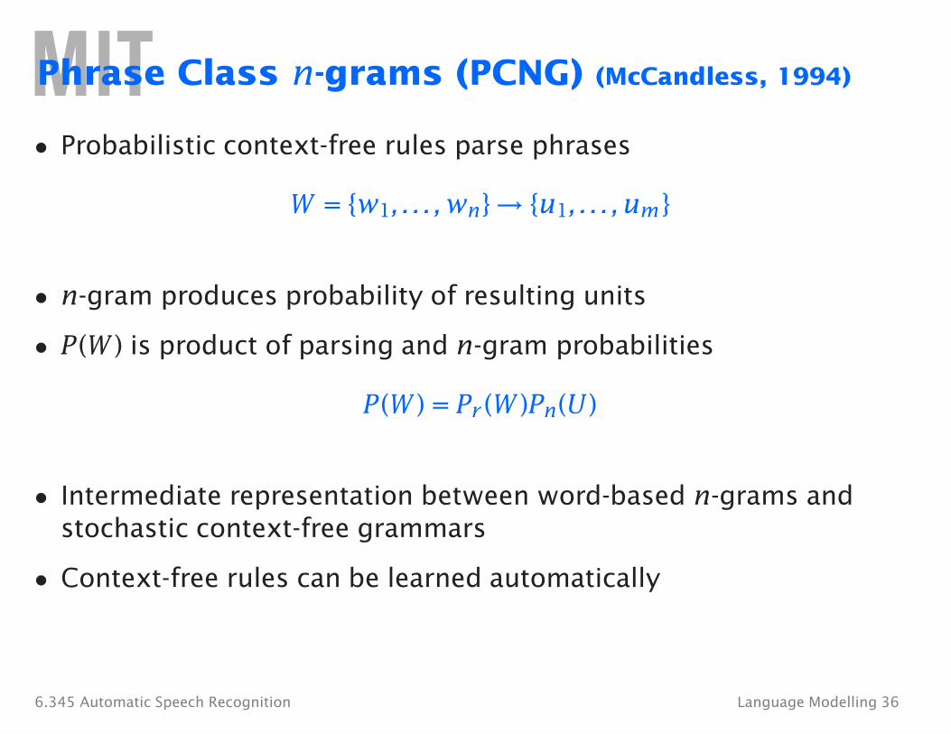
• P. Brown et al., Class-based n-gram models of natural language, Computational Linguistics, 1992.

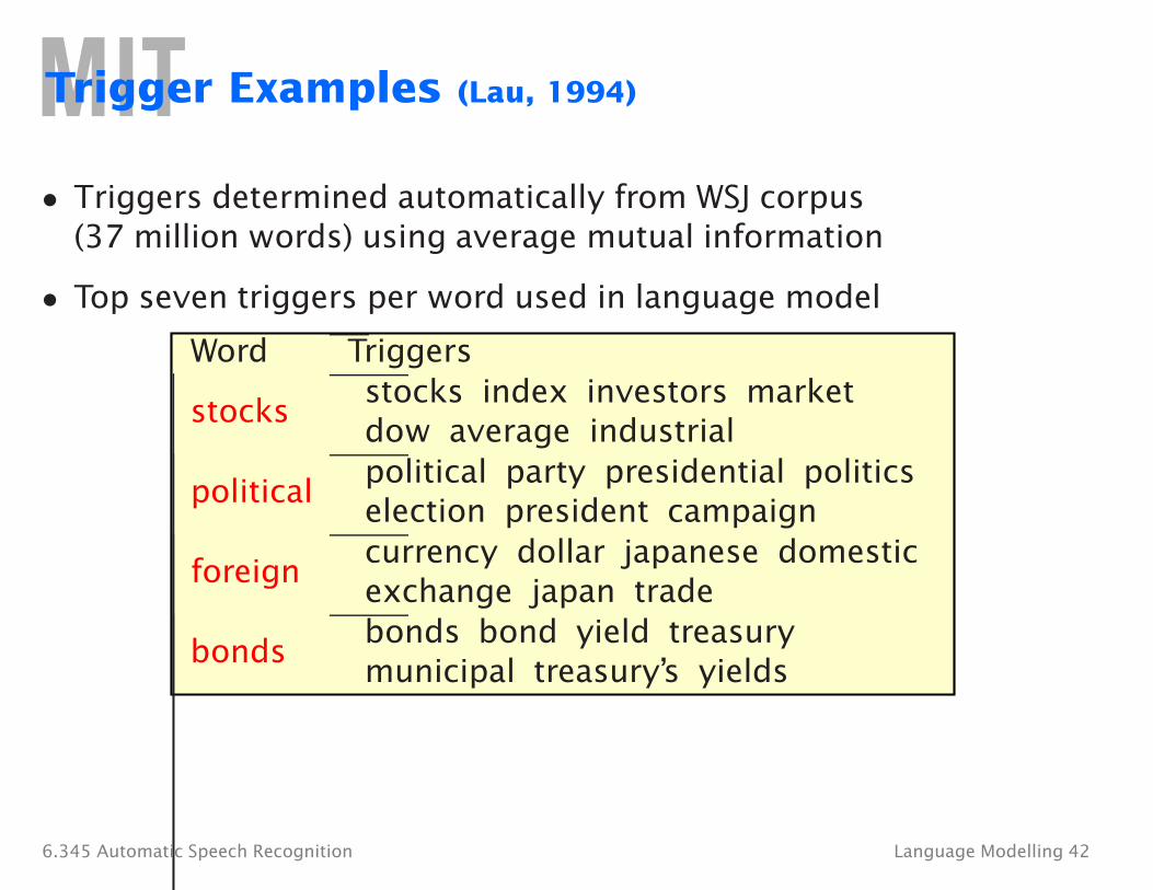
• R. Lau, Adaptive Statistical Language Modelling, S.M. Thesis, MIT, 1994.

• M. McCandless, Automatic Acquisition of Language Models for Speech Recognition, S.M. Thesis, MIT, 1994.

• R. Rosenfeld et al., Language Modelling for Spontaneous Speech, Johns Hopkins Workshop, 1995.

• A. Stolcke, Entropy-based Pruning of Backoff Language Models, http://www.nist.gov/speech/publications/darpa98/html/lm20/lm20.htm, 1998.


Date post:	18-Mar-2018
Category:	Documents
Upload:	vankien
View:	216 times
Download:	2 times

S Evaluation Language Modelling for R - MIT OpenCourseWare · PDF fileLanguage Model R...

Documents