S-wave Velocity Structure of Mexico City Obtained from Three-component

Microtremor Measurements and Microtremor Array Measurements

Koichi Hayashi*, Geometrics Atsushi Nozu, Port and Airport Research Institute,

Masanori Tanaka, Port and Airport Research Institute Haruhiko Suzuki, OYO Corporation

Efraín Ovando Shelley, Universidad Nacional Autonoma de Mexico

1

Outline • Introduction

• Investigation site

• Data acquisition Equipment H/V spectrum Dispersion curve

• Analysis results

• Comparison with United States

• Conclusions

2

Introduction • The earthquake that struck Mexico on 19 September

1985 caused severe damage in Mexico City although the city is located 400km away from the epicenter.

• The main reason for this damage is that the city is located on a basin filled with very soft sediments.

• Distribution of these soft sediments has been delineated by drillings and microtremor measurements.

• A small number of attempts have been made to image the S-wave velocity structure of the basin using downhole seismic loggings.

• In order to delineate S-wave velocity structure of the basin down to depth of approximately 200m, we have performed three-component micro-tremor measurements and microtremor array measurements.

3

1985 Mexico Earthquake

4

Mexico City

Mw=8.3

400km

1985 Mexico Earthquake • Mw=8.3

• Most-often cited number of deaths is an estimated 10,000 people but experts agreed that it could be up to 40,000.

• Damage area corresponds to the western part of the lake zone within 2 to 4 kilometers of the Alameda Central.

• 6 to 15 story buildings are mainly damaged in the city due to a frequency range of 0.25 to 0.5Hz (period of 2 to 4seconds)

5

> 2sec

Natural Period (H/V) of Mexico Basin

6

Lermo and Chavez-Garcia (1994)

Central Mexico City

Airport

Damage Area

> 4sec

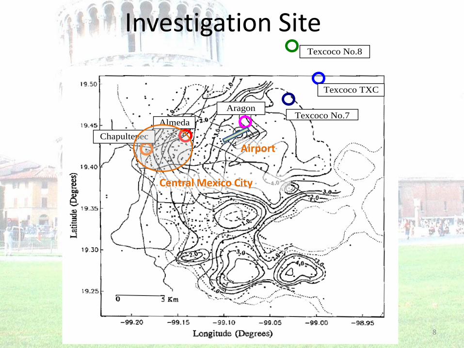
Investigation Site

• Investigation site is placed at the downtown of Mexico City.

• 30km length survey line crosses the basin with a west-southwest to east-northeast direction.

• 3 component microtremor measurements were performed at more than 10 sites on the line.

• Microtremor array measurements were performed at 6 sites on the line.

• Microtremor array measurements used 25 to 650m equilateral triangular arrays.

7

Chapultepec

Aragon Texcoco No.7

Almeda

Texcoco No.8

Texcoco TXC

Investigation Site

Central Mexico City

Airport

8

Example of Array Configuration

19.422938 -99.182564

19.423838 99.184163

19.423818 99.180783

19.42138 99.182296

330m

19.462283 99.067562

19.463962 99.066875

19.4629 99.063903

19.464731 99.069911

19.461818 99.06931

19.460988 99.066317

19.459238 99.068806

650m

Chapultepec Aragon

9

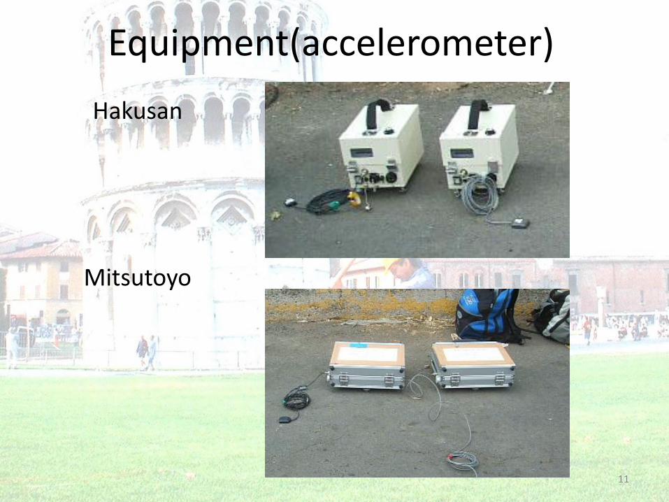
Data Acquisition • Data acquisition was carried out during the daytime in

December 2008 and December 2009. • Microtremor measurement systems (JU210) made by

Hakusan Corporation and data loggers (GPL-6A3P) made by Mitsutoyo Corporation were mainly used for data acquisition.

• Both systems use accelerometers for the sensors. • In order to verify applicability of the accelerometers, servo-

type velocity meters made by Katsujima Corporation (SD-110) and Tokyo Sokushin Corporation (VSE11F, VSE12F) were also used in the 3 component microtremor measurements.

• H/V spectra obtained through the accelerometers and the velocity meters were compared.

• 30 min. to 1 hour of microtremors were recorded for each three component measurement or array measurement.

10

Equipment(accelerometer)

11

Hakusan

Mitsutoyo

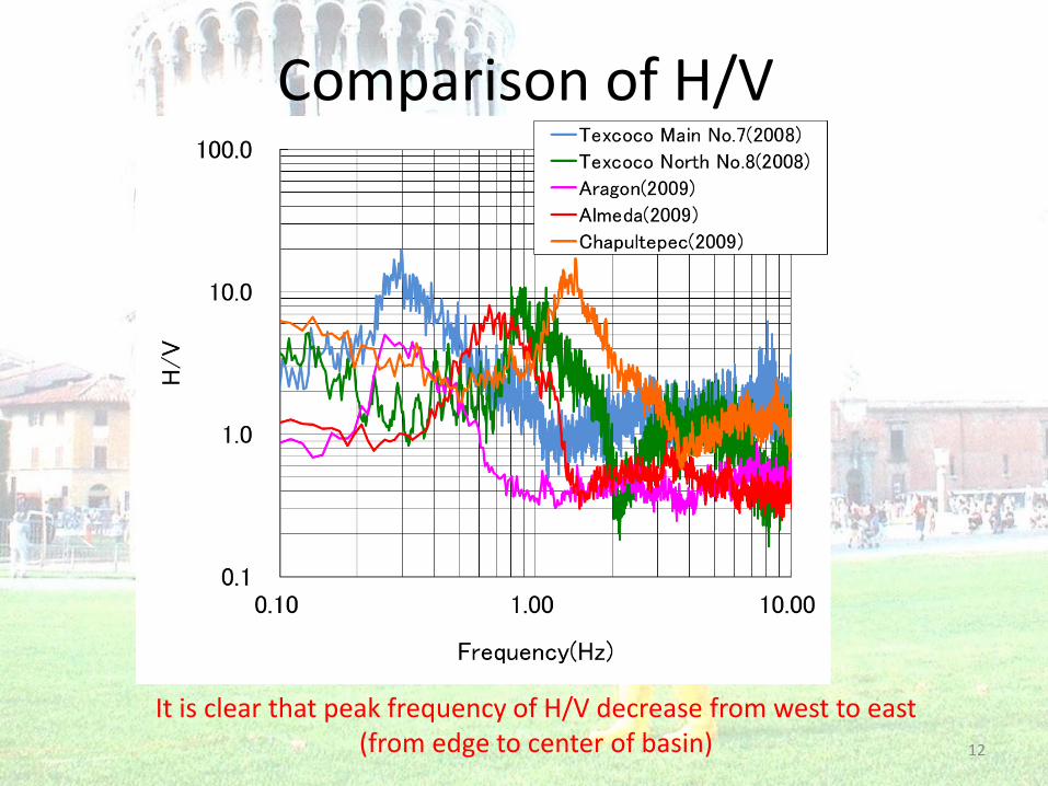
Comparison of H/V

It is clear that peak frequency of H/V decrease from west to east (from edge to center of basin) 12

Comparison of Dispersion Curve

Sites where the peak frequency of H/V spectra is higher, the phase velocity of the dispersion curve is also higher 13

Analysis (1) • A joint inversion was applied to the observed

H/V spectra and dispersion curves, and S-wave velocity models were analyzed for six sites.

• In the inversion, phase velocities of the dispersion curves and peak frequencies of the H/V spectra were used as the observation data.

• Unknown parameters were layer thickness and S-wave velocity.

• A Genetic algorithm was used for optimization.

14

Analysis (2) • Initial models were created by a simple

wavelength transformation in which wavelength calculated from phase velocity and frequency is divided by three and plotted at depth.

• Theoretical H/V spectra and phase velocities are generated by calculating the weighted average of the fundamental mode and higher modes (up to the 4th modes) based on medium response.

• Rayleigh-Love ratio (R/L) is fixed as 0.7 15

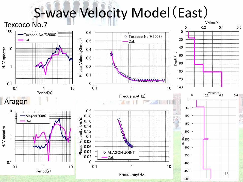
Texcoco No.7 S-wave Velocity Model（East）

Aragon 0

50

100

150

200

250

300

350

400

450

500

0 0.2 0.4 0.6Vs(km/s)

Depth(m)

16

S-wave Velocity Model（West） Almeda

Chapultepec

17

Chapultepec

Aragon Texcoco No.7

Almeda

Texcoco No.8

Texcoco TXC

Peak Frequency of H/V and S-wave Velocity Model

0.7s

90m/s

1.5s

80m/s

3.9s

60m/s

3.3s

30m/s

1.1s

60m/s

＞400m/s 450m

<100m/s

≒200m/s

18

Comparison with United States H/V Spectra Dispersion Curve S-wave Velocity Model

S-wave velocity of Mexico is extremely low compare with San Jose and Redwood City.

Mexico City San Jose (William St. Park), CA Redwood City, CA

19

0

50

100

150

200

250

300

350

0.1 1 10 100

Phas

e-vel

oci

ty(m

/sec

)

Frequency(Hz)

Mexico

San Jose

Redwood City

0.1

1

10

0.1 1 10

H/V

spec

tra

Period(sec)

Mexico

San Jose

Redwood City

0

20

40

60

80

100

120

140

160

0 100 200 300 400 500

Dep

th (

m)

S-wave velocity (m/sec)

Mexico

San Jose

Redwood City

Conclusions • We have performed the three-component

microtremor measurements and microtremor array measurements in the Mexico basin and estimated the S-wave velocity models down to a depth of 200m.

• S-wave velocity in the middle of the Mexico basin is lower than 150m/s to a depth of 70m and much lower than typical alluvial plains in Japan and United States.

• Peak frequencies of the H/V spectra in Mexico City vary from 0.25 to 1Hz and it seems that these peak frequencies are mainly due to the low-velocity layer shallower than a depth of 100m.

20