Acknowledgement Many helpful hands have contributed to this study. Thanks go to William Hurst for the technical help with the equipment installation, maintenance, and collection and storage of the wind data; Bob Eldridge and Terence Lennie for collecting the wind data at the site in Sachs Harbour, and many others for facilitating the wind monitoring effort. Acknowledgement is also given to Annika Trimble and Pippa Seccombe-Hett for editing the report. This study was carried out with contributions from Environment and Natural Resources, and the Aurora College.
Executive Summary The Hamlet of Sachs Harbour has a population of about 120 people and is located at the southwest coast of Banks Island in the Amundsen Gulf. The diesel-electric power plant in Sachs Harbour, as well as the distribution system, is owned and operated by the Northwest Territories Power Corporation. The plant supplies 907 MWh/year of electricity with an average load of about 104 kW. The maximum and minimum loads are 209 kW and 68 kW, respectively.
In July 2005, two wind monitoring stations were installed in the community: one was set up 6.5 km west of the centre of the hamlet; and for the other a set of heated sensors was installed at the site where an AOC 50 wind turbine (now EW50) used to operate. The wind data analysis shows a long-term annual mean wind speed of 5.4 and 6.6 m/s at 10- and 37 m above ground level (AGL) at the heated site (by the original wind turbine foundation). The tallest tower available for a small scale wind development suitable for this community is 37 m tall, such as the EW50 turbine by Entegrity, which is used for the economic analysis in this study.
Accordingly, the wind analysis and modelling is focused towards estimating winds at 37 m above ground level. Three sites are considered for this study: the original wind turbine site, and new proposed Sites #1 and #2 which are both east of the hamlet and along the edge of the bluff overlooking Amundsen Gulf to the south. Based on the wind analysis and numerical modeling, the long-term annual mean wind speeds for these proposed sites are 6.6, 6.5, and 6.6 m/s, respectively.
Developing a wind project at the former AOC site with a new turbine on a 25 metre tower (at which the wind speed is estimated to be 6.2 m/s) on the existing foundation would cost $382,000, or $5,877 per kW. With a 37 metre tower the former AOC site with new turbine on a new foundation would cost $464,500, or $7,146 per kW. Both the 25m and 37m AGL scenarios were run and were calculated to produce power at $0.464 per kWh. Compared to a fuel cost of $0.469 per kWh, this means that the wind turbine is feasible without any subsidies.
Site # 1 was estimated to cost $786,500 or $12,100 per kW to develop and the cost to produce power is $0.731 per kWh, about 56% more expensive than the avoided cost of diesel. Site #2 will cost about $704,500 or $10,838 per kW to develop with an estimated cost to produce power at $0.645 per kWh which is still about 38% more expensive than the avoided cost of diesel.
Reducing the interest cost (cost of capital) from 8% to 4% would reduce the cost of wind generated electricity at the original AOC turbine site (and from incremental turbines at the other two sites) to about $0.37 - $0.39 per kWh - essentially the same as the cost of diesel generated power indicated in NTPC’s wind power request for proposals ($0.37 per kWh).
With its excellent wind resource and high cost of electricity production, Sachs Harbour is an excellent candidate for developing a wind project. The hamlet leadership should seriously consider developing one at the original AOC site or else seek subsidies to develop power lines to the other sites proposed.
Background JP Pinard, P.Eng., Ph.D. and John Maissan, P.Eng. of Leading Edge Projects Inc. (the authors) have been retained by the Aurora Research Institute to conduct a pre-feasibility study for wind energy generation in Sachs Harbour. This study examines wind data from the airport stations, wind monitoring stations, maps, satellite images and makes use of a computer windflow model to identify potential wind monitoring sites around the community. This study provides the information listed below:
1) An analysis of wind data to estimate long-term mean wind speed and direction; 2) Estimates of the wind speeds around the hamlet generated with computer models; 3) A list of potential sites for location of wind equipment; 4) A description of the power system in the hamlet which includes the size, capacity and
condition of present system; 5) An analysis of different scenarios of power demands for the hamlet; 6) Preliminary estimates of the cost of wind generation for the hamlet; 7) Estimates of power production and fuel displacement through integration of wind power; 8) An outline of next steps needed to pursue the integration of wind power in the hamlet.
Acronyms AGL – above ground level
ASL – above sea level
CS – Climate station, refers to the 24-hour Auto station at the airport
GHG – greenhouse gas
NTPC – Northwest Territories Power Corporation
NTCL – Northern Transportation Company Limited
MCP – Measure-Correlate-Predict, a method for projecting short-term wind measurements to long-term using nearby long-term weather stations such as those at the airport.
WM – wind monitoring site, refers to the site where the wind measurements for wind energy purposes are made.
Introduction The Hamlet of Sachs Harbour has a population of about 120 people and is located at the southwest coast of Banks Island in the Amundsen Gulf (see Figure 1). The Inuvialuit community is 1150 km northwest of Yellowknife and is accessible by air and by barge.
A diesel-electric generating plant that is owned and operated by the Northwest Territories Power Corporation (NTPC) supplies the electrical energy for Sachs Harbour. There has been interest expressed in displacing the diesel energy with renewable energy.
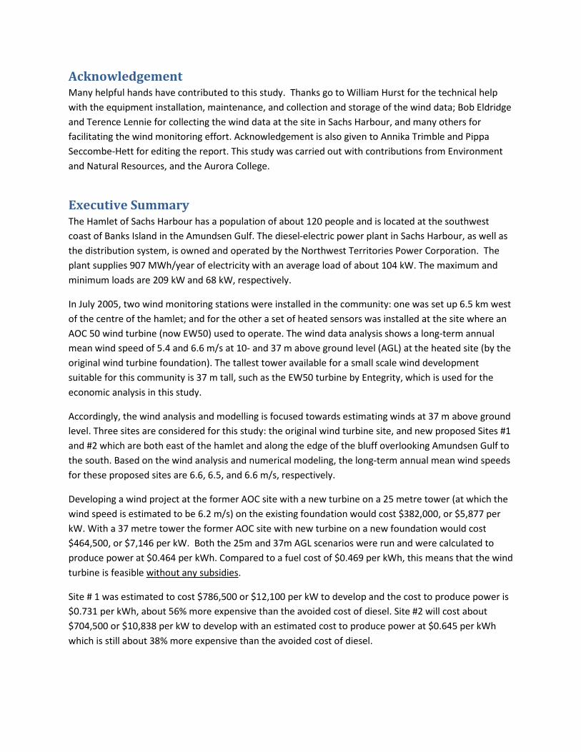
In July 2005, two wind monitoring stations were installed around the community: one was set up 6.5 km west of the centre of the hamlet; and for the other a set of heated sensors was installed at the site where an AOC 50 wind turbine used to operate (Figure 2). A progress report (Pinard, 2007) was produced to evaluate the mean wind climate of the area, and the mean annual wind speed at the site in the hamlet revealed very promising winds at 7.6 m/s (projected to 30 m above the surface).
The purpose of this report is to examine the potential for wind power generation by providing a selection of potential sites, estimating the mean annual wind speed and estimating the economics of building a wind installation near the hamlet. The focus of this study is also to determine the best possible sites within one km of the hamlet power grid. While the western wind monitoring station provides good information such as vertical profiles, it is too far from the community. Thus, the focus will remain with the heated station and the auto station at the airport.
Figure 1: The location of Sachs Harbour in relation to the rest of Canada.
Sachs Harbour
The Wind Data Collecting Stations There are two wind monitoring stations that were set up in Sachs Harbour. The first is a 30 m tower with 3 wind speed sensors, or anemometers, set at 10-, 20-, and 30 m AGL on the tower. The booms (1.1 m long) attaching each anemometer to the tower, point to the east-southeast. A wind vane is installed at the tower top on a boom pointing west-southwest. A temperature sensor is at the bottom. This wind monitoring station is located at the west end of the hamlet near the dump and has been running since June 24, 2005. Data from this station was used in this study up to January 2009.
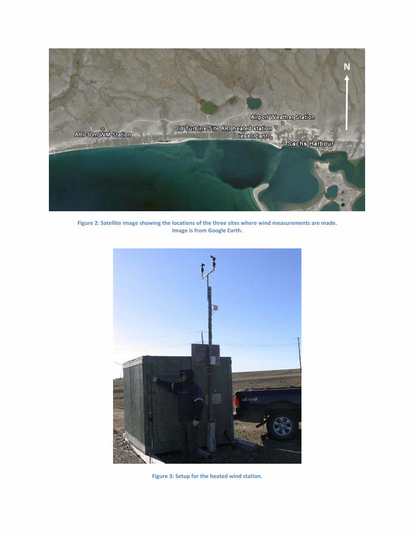
The second station which was set up consists of heated sensors (see Figure 3) at the top of a pipe attached to a hut. The sensors are NRG IceFreeII models and rest at 4.2 m AGL. They are connected to the local grid via the hut’s power line, which was originally used for connecting the AOC wind turbine that was formerly installed at this site. It has been found in a study by Landberg (2000) that wind speed sensors placed over the top of the hut may be affected by localized overspeeding because the hut’s dimensions act as a hill. This is addressed in a proceeding section, and will require adjusting (reducing) the measured wind speed at the heated station.
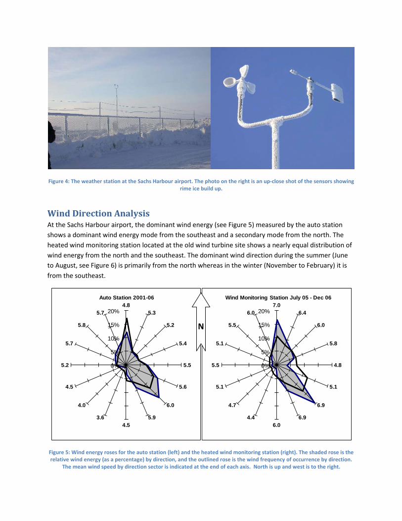
At the airport there are apparently two stations that measure the wind speed at 10 m AGL. Only one station, however, was found and it is shown in Figure 4. The weather data for both stations are stored at Environment Canada’s website. The automated station, or “auto” station (also called CS: climate station), at 87.5 m ASL has monitored weather conditions 24 hours a day since 1994 and stores the data directly to a data logger. The other airport station (86 m ASL), designated with the letter A, is typically monitored during office hours and its data is recorded at the top of each hour. The airport A station has collected data since 1955.The hourly wind data from the stations at the airports that are used for this analysis originate from monthly files, which have been downloaded from the Environment Canada’s website.
The locations of the three measurement stations are shown in Figure 2.
Figure 2: Satellite image showing the locations of the three sites where wind measurements are made. Image is from Google Earth.
Figure 3: Setup for the heated wind station.
N
Figure 4: The weather station at the Sachs Harbour airport. The photo on the right is an up-close shot of the sensors showing rime ice build up.
Wind Direction Analysis At the Sachs Harbour airport, the dominant wind energy (see Figure 5) measured by the auto station shows a dominant wind energy mode from the southeast and a secondary mode from the north. The heated wind monitoring station located at the old wind turbine site shows a nearly equal distribution of wind energy from the north and the southeast. The dominant wind direction during the summer (June to August, see Figure 6) is primarily from the north whereas in the winter (November to February) it is from the southeast.
0%
5%
10%
15%
20%4.8
5.3
5.2
5.4
5.5
5.6
6.0
5.94.5
3.6
4.0
4.5
5.2
5.7
5.8
5.7
Auto Station 2001-06
0%
5%
10%
15%
20%7.0
6.4
6.0
5.8
4.8
5.1
6.9
6.96.0
4.4
4.7
5.1
5.5
5.1
5.5
6.0
Wind Monitoring Station July 05 - Dec 06
Figure 5: Wind energy roses for the auto station (left) and the heated wind monitoring station (right). The shaded rose is the relative wind energy (as a percentage) by direction, and the outlined rose is the wind frequency of occurrence by direction.
The mean wind speed by direction sector is indicated at the end of each axis. North is up and west is to the right.
N
Jul0°
30°
60°
90°
120°
150°180°
210°
240°
270°
300°
330°
10%
20%
30%
Feb0°
30°
60°
90°
120°
150°180°
210°
240°
270°
300°
330°
10%
20%
30%
Figure 6: Wind energy roses for the heated wind monitoring station shows the dominant wind direction tendencies in the summer (July) and the winter (February).
Wind Speed Analysis
Defining the Long-term Mean in Sachs Harbour The airport A and the auto station are compared to each other for the period 2001-06. During this period the auto station had an annual mean wind speed of 5.36 m/s and the airport A station was 5.23 m/s (approximately 2% less).
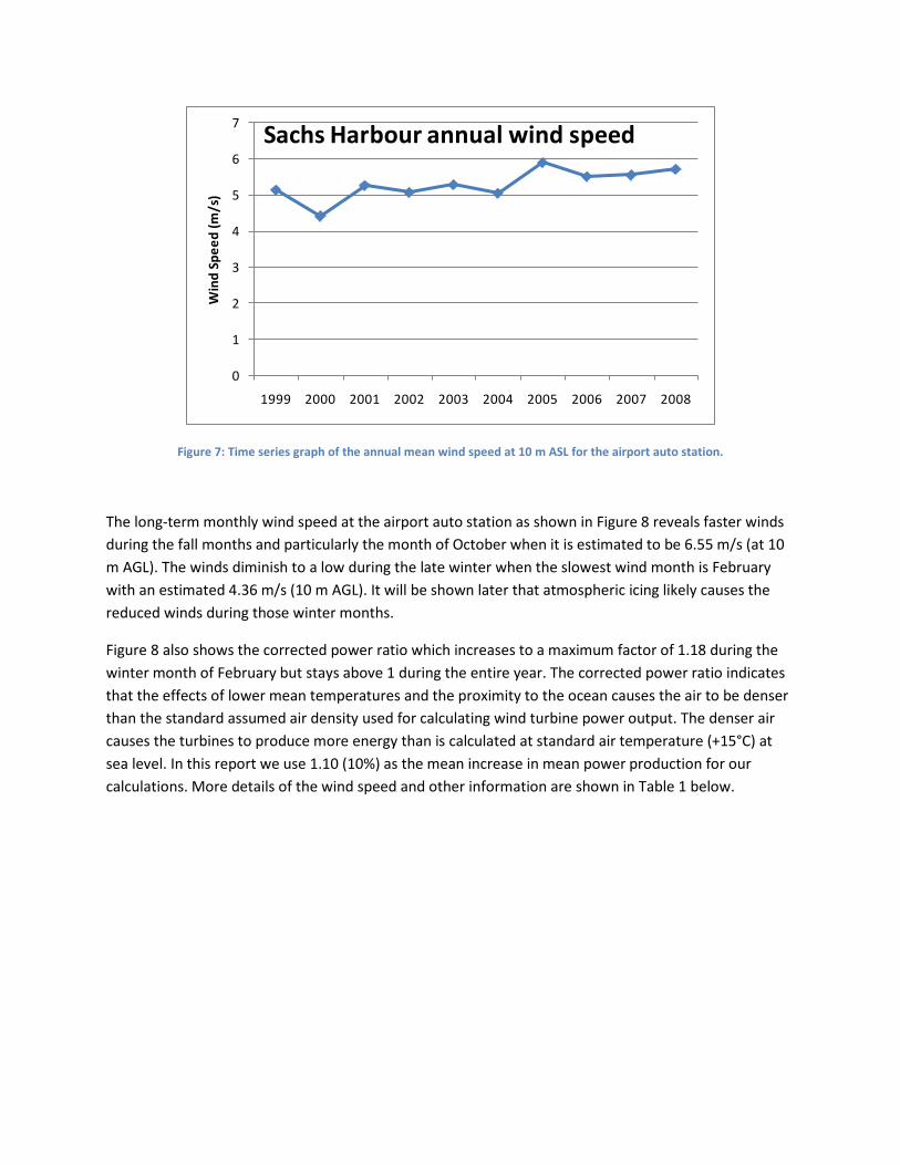
The auto station recorded the most recent 5-year (2004-08) mean wind speed of 5.55 m/s, and a ten-year (1999-2008) mean wind speed of 5.29 m/s. The standard deviation of the mean annual wind speed about the 10-year mean is 0.42 m/s. Figure 7 shows a time series of the annual mean speeds for the last ten-years. Although it shows a trend of increasing wind speed there may other longer term variabilities such as those due to ocean water temperature oscillations like the Arctic Decadal Oscillation (see Bond, 2009) at play. For the purpose of this study, using the ten-year mean should provide a conservative estimate of the mean wind speed for the area. Because of its 24-hour availability, the auto station wind data is used for the comparative analysis with the wind monitoring data.
N
0
1
2
3
4
5
6
7
1999 2000 2001 2002 2003 2004 2005 2006 2007 2008
Win
d Sp
eed
(m/s
)
Sachs Harbour annual wind speed
Figure 7: Time series graph of the annual mean wind speed at 10 m ASL for the airport auto station.
The long-term monthly wind speed at the airport auto station as shown in Figure 8 reveals faster winds during the fall months and particularly the month of October when it is estimated to be 6.55 m/s (at 10 m AGL). The winds diminish to a low during the late winter when the slowest wind month is February with an estimated 4.36 m/s (10 m AGL). It will be shown later that atmospheric icing likely causes the reduced winds during those winter months.
Figure 8 also shows the corrected power ratio which increases to a maximum factor of 1.18 during the winter month of February but stays above 1 during the entire year. The corrected power ratio indicates that the effects of lower mean temperatures and the proximity to the ocean causes the air to be denser than the standard assumed air density used for calculating wind turbine power output. The denser air causes the turbines to produce more energy than is calculated at standard air temperature (+15°C) at sea level. In this report we use 1.10 (10%) as the mean increase in mean power production for our calculations. More details of the wind speed and other information are shown in Table 1 below.
0.90
0.95
1.00
1.05
1.10
1.15
1.20
2.0
2.5
3.0
3.5
4.0
4.5
5.0
5.5
6.0
6.5
7.0
Jan Feb Mar Apr May Jun Jul Aug Sep Oct Nov Dec
Corr
ecte
d Po
wer
Rat
io
Win
d Sp
eed
(m/s
)
Airport(10m)
Corrected Power Ratio
Figure 8: Long-term monthly means of the corrected power ratio and wind speed based on the ten-year (1999-2008) airport auto station data measured at 10 m AGL. The wind speed is referenced to the left side and the air density to the right.
Table 1: Monthly mean values based on airport auto station measurements for the period 2001-2008. The wind speeds are measured at 10 m above ground level (AGL).
Wind Speed Temperature Pressure Density Corrected (m/s) (°C) (kPa) (kg/m3) Pow er Ratio
Comparing the Wind Speed from the Auto and Wind Monitoring Stations The period chosen for the comparative study is approximately 3.5 years, from 8 July, 2005 to January 2009.
The wind speed correlation between the measurements from the 30 m unheated wind monitoring site and the auto station was (Pearson) R= 0.87 when comparing the 30 m wind sensor to the auto 10 m
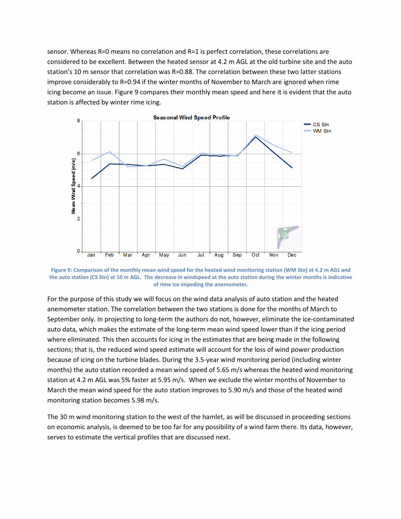
sensor. Whereas R=0 means no correlation and R=1 is perfect correlation, these correlations are considered to be excellent. Between the heated sensor at 4.2 m AGL at the old turbine site and the auto station’s 10 m sensor that correlation was R=0.88. The correlation between these two latter stations improve considerably to R=0.94 if the winter months of November to March are ignored when rime icing become an issue. Figure 9 compares their monthly mean speed and here it is evident that the auto station is affected by winter rime icing.
Figure 9: Comparison of the monthly mean wind speed for the heated wind monitoring station (WM Stn) at 4.2 m AGL and the auto station (CS Stn) at 10 m AGL. The decrease in windspeed at the auto station during the winter months is indicative
of rime ice impeding the anemometer.
For the purpose of this study we will focus on the wind data analysis of auto station and the heated anemometer station. The correlation between the two stations is done for the months of March to September only. In projecting to long-term the authors do not, however, eliminate the ice-contaminated auto data, which makes the estimate of the long-term mean wind speed lower than if the icing period where eliminated. This then accounts for icing in the estimates that are being made in the following sections; that is, the reduced wind speed estimate will account for the loss of wind power production because of icing on the turbine blades. During the 3.5-year wind monitoring period (including winter months) the auto station recorded a mean wind speed of 5.65 m/s whereas the heated wind monitoring station at 4.2 m AGL was 5% faster at 5.95 m/s. When we exclude the winter months of November to March the mean wind speed for the auto station improves to 5.90 m/s and those of the heated wind monitoring station becomes 5.98 m/s.
The 30 m wind monitoring station to the west of the hamlet, as will be discussed in proceeding sections on economic analysis, is deemed to be too far for any possibility of a wind farm there. Its data, however, serves to estimate the vertical profiles that are discussed next.
Projecting to Higher Levels Turbulent air flow over rough surfaces tend to generate a vertical profile of horizontal winds that are fairly predictable and are dependent on neutral, well-mixed air conditions and the roughness of the ground surface. This vertical profile is defined by:
where u1 is the known wind speed at z1 (typically at 10 m AGL), and is projected to u2 at the height z2. The surface roughness is defined by zo which as a rule of thumb is 1/10 the height of the grass or brush surrounding the site where the measurements are made. The extent of the influence of the surface roughness and the log equation is typically up to approximately 100m. If we know the wind speeds at two heights of say 10 and 30 m then we can also find the value of zo and compare that to roughness charts to confirm that measurements are reasonable.
In the Sachs Harbour area the land surface is typically tundra, with slightly undulating terrain and depressions that fill with snow during the winter (hence smoothing the surface and reducing zo). The surface roughness is expected to be between 0.01 m (1 cm), which is the equivalent of an airport runway area, to 0.1 m (10 cm), which represents a roughly open area with a few obstacles. A previous report (Pinard, 2007) the surface roughness zo was calculated to be 0.005 m (0.5 cm) which is considered to be the smoothness of a snow-covered flat field. With the longer set of measurements, the new calculations of the surface roughness result in zo = 0.02 m. Using this value for zo we can calculate the log profile that is shown in Figure 10 as “U (log)” and which is superimposed over the measurements “U (msd)” that were made by the 30 m station to the west.
Projecting to a Longer Term As is noticeable from Figure 7, the annual mean wind speed in the last few years has been rather high compared to the last 10 years. From the 3.5-year period in 2005-08 to the longer 10-year period the auto station’s mean wind speed decreases to 90% of its short-term values. This means that we must adjust the wind monitoring measurements down as well. A simple way to do this is multiply the value by, in this case, 0.90. A slightly more complicated, however more elegant, method is in the following text.
The vertical profile U(log) shown in Figure 10 is adjusted to an eight-year mean “U (long-term)” using the MCP method of measuring, correlating, and predicting the long-term mean winds. The formula is:
,
where Es is the estimated long term wind speed at the site of the wind monitoring station, µs is the measured wind speed at the site, µr is the measure reference wind speed, and Er is the measured long-term mean wind speed at the reference station. The other variables in the equation are the correlation
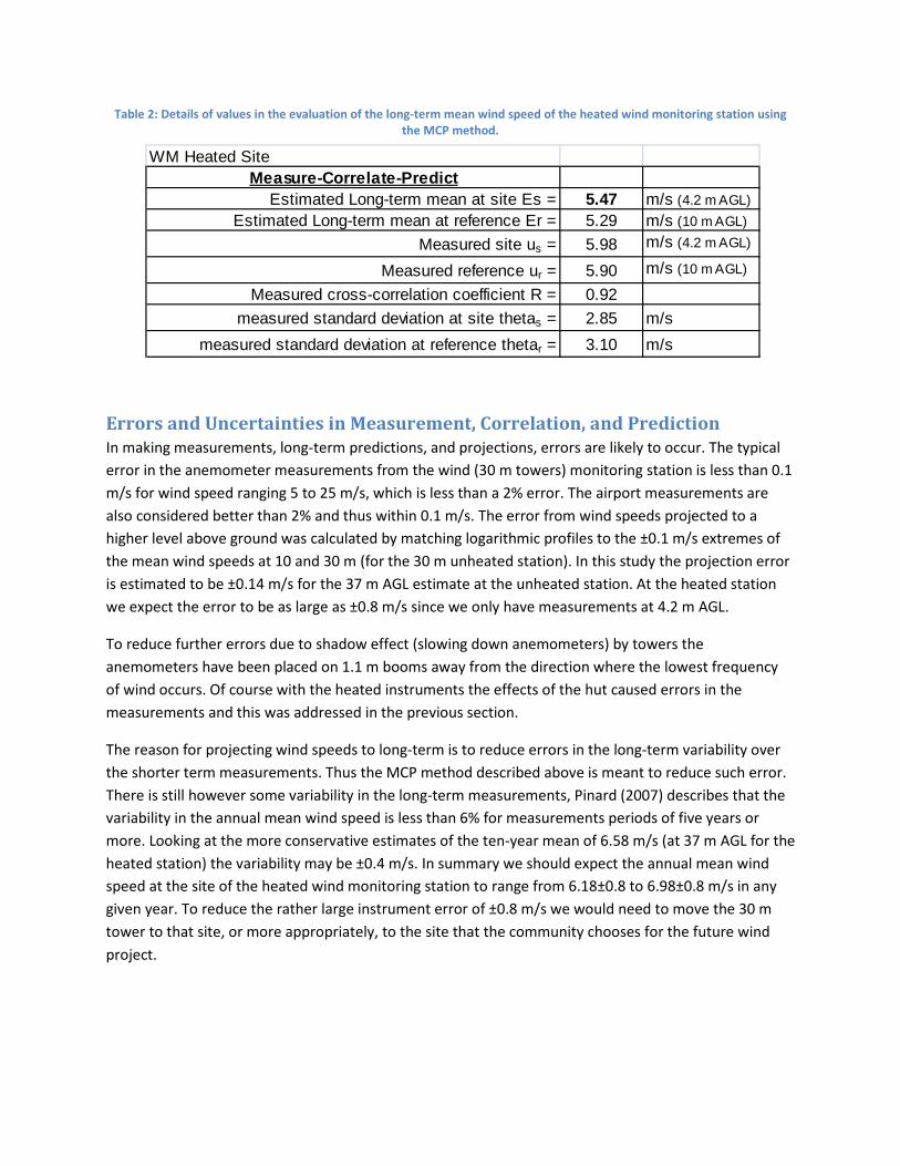
coefficient R and the standard deviation for the reference station, σr, and the wind monitoring site, σs. The values are listed in Table 2 and so from the equation above, the estimated long-term mean annual wind speed at the heated wind monitoring station is 5.47 m/s at 4.2 m AGL.
0
10
20
30
40
50
60
70
0 1 2 3 4 5 6 7
Hei
ght
abov
e gr
ound
leve
l (m
)
Mean Wind Speed (m/s)
U (log)
U (msd)
U(unhtd) 10-yr
U(htd) 10-yr
Figure 10: Vertical profiles of the horizontal mean wind speed at the unheated 30 m and heated wind monitoring sites. The vertical profile “U (log)” is fitted to the measurements “U (msd)” of the unheated 30 m station and then adjusted to the long-term 10 year [U (unhtd) 10-yr] projections. Black whiskers associated with “U (msd)” indicate possible errors of ±0.1 m/s due
to sensor inaccuracies. U (htd) 10-yr indicates long-term mean wind speed projections made at the heated station for different heights AGL.
As stated earlier we must consider the effect of the building on the wind speed measurements of the heated sensor. The hut is a cube of about 2 m dimension and the wind sensor is 2.2 m above the building. Using the measurements made in Landsberg (2000), the mean wind speed-up caused by the building on the tower that is one building height above it is estimated to be about 1.17 or 17% of the mean wind speed without the building. The measured wind speed of 5.47 m/s is divided by 1.17 to obtain 4.68 m/s. If we project this value to 10 m AGL using a multiplier of 1.162 (obtained from the 30 m wind monitoring data discussed below) this brings the wind speed up to 5.43 m/s, which is about 3% higher than the 10-year mean of 5.29 m/s measured at the airport at the same level AGL.
From the above two formulae, the 10-year (1999-2008) projected mean of the heated site at 37 m AGL is 6.58 m/s. The vertical profiles of estimated long-term means for the both the heated and unheated wind monitoring sites are shown in Figure 10 and listed in Table 3.
Table 2: Details of values in the evaluation of the long-term mean wind speed of the heated wind monitoring station using the MCP method.
WM Heated SiteMeasure-Correlate-Predict
Estimated Long-term mean at site Es = 5.47 m/s (4.2 m AGL)Estimated Long-term mean at reference Er = 5.29 m/s (10 m AGL)
Measured site us = 5.98 m/s (4.2 m AGL)
Measured reference ur = 5.90 m/s (10 m AGL)
Measured cross-correlation coefficient R = 0.92measured standard deviation at site thetas = 2.85 m/s
measured standard deviation at reference thetar = 3.10 m/s
Errors and Uncertainties in Measurement, Correlation, and Prediction In making measurements, long-term predictions, and projections, errors are likely to occur. The typical error in the anemometer measurements from the wind (30 m towers) monitoring station is less than 0.1 m/s for wind speed ranging 5 to 25 m/s, which is less than a 2% error. The airport measurements are also considered better than 2% and thus within 0.1 m/s. The error from wind speeds projected to a higher level above ground was calculated by matching logarithmic profiles to the ±0.1 m/s extremes of the mean wind speeds at 10 and 30 m (for the 30 m unheated station). In this study the projection error is estimated to be ±0.14 m/s for the 37 m AGL estimate at the unheated station. At the heated station we expect the error to be as large as ±0.8 m/s since we only have measurements at 4.2 m AGL.
To reduce further errors due to shadow effect (slowing down anemometers) by towers the anemometers have been placed on 1.1 m booms away from the direction where the lowest frequency of wind occurs. Of course with the heated instruments the effects of the hut caused errors in the measurements and this was addressed in the previous section.
The reason for projecting wind speeds to long-term is to reduce errors in the long-term variability over the shorter term measurements. Thus the MCP method described above is meant to reduce such error. There is still however some variability in the long-term measurements, Pinard (2007) describes that the variability in the annual mean wind speed is less than 6% for measurements periods of five years or more. Looking at the more conservative estimates of the ten-year mean of 6.58 m/s (at 37 m AGL for the heated station) the variability may be ±0.4 m/s. In summary we should expect the annual mean wind speed at the site of the heated wind monitoring station to range from 6.18±0.8 to 6.98±0.8 m/s in any given year. To reduce the rather large instrument error of ±0.8 m/s we would need to move the 30 m tower to that site, or more appropriately, to the site that the community chooses for the future wind project.
Table 3: Details of measurements and their projection to long-term and to higher elevations. Bold values indicate the estimated long-term (1999-2008) mean wind speed for the unheated 30-m and heated wind monitoring stations. These
values are also shown in Figure 10 above as “U (unhtd) 10-yr” and “U (htd) 10-yr”.
Location and measurement period Height Wind speedSachs Harbour Auto 8 July 05 to Sept 08 10 m AGL 5.60 m/sSachs unheated WM 8 July 05 to Sept 08 10 m AGL 5.00 m/s
20 m AGL 5.42 m/s30 m AGL 5.75 m/s
Auto station mean compared to heated 10 m AGL 5.90 m/sSachs Heated WM 8 July 05 to Sept 08 4.2 m AGL 5.98 m/s
Sachs Harbour Auto 10-year 1999-2008 average 10 m AGL 5.29 m/sRatio of 2005-08 to ten-year mean 0.90
Sachs H. WM wind projected to ten-years at 10 m AGL 4.64 m/sBased on unheated 30-m tower sensors 20 m AGL 5.16 m/s
30 m AGL 5.47 m/s37 m AGL 5.62 m/s40 m AGL 5.68 m/s50 m AGL 5.85 m/s60 m AGL 5.98 m/s
Sachs H. WM wind projected to ten-years at 4.2 m AGL 5.47 m/sadjusted for building 4.2 m AGL 4.68 m/sBased on the heated sensors at 4.2 m 10 m AGL 5.43 m/s
20 m AGL 6.04 m/s30 m AGL 6.39 m/s37 m AGL 6.58 m/s40 m AGL 6.65 m/s50 m AGL 6.84 m/s60 m AGL 7.00 m/s
Possible Locations for a Wind Farm in Sachs Harbour As noted earlier, the wind monitoring station that is approximately 6.5 km west of the hamlet is too far simply because the cost of power lines as will be shown later. The focus for a wind farm location is at least within one km of power line, and the closer the better. The restriction, however, is that the wind farm must not interfere with the safety and the communication systems of the airport. The wind farm must also be a reasonable distance away from the community residences. One site other than that of the old wind turbine was proposed by local authorities and it is in a gravel quarry just east of the community. That site is illustrated as Site #1 in Figure 11. To find out whether this or any other site would be suitable for a wind farm we use numerical modeling validated by the measurements.
Numerical Modeling with MS-Micro Since we only have two locations in the hamlet area where wind speeds are measured we need other tools to help estimate the mean wind speed at other locations. To achieve this we use a numerical wind modeling tool called MS-Micro. Originally based on boundary-layer wind field theories of Jackson and Hunt (1975), it was modified and made into a useable computer wind modeling tool by Walmsley et al. (1986). The theory of MS-Micro has been used widely in the wind energy industry under the cloaks of WaSP and Anemoscope.
MS-Micro is run for the Sachs Harbour area using data elevations of ~20 m resolution from the Geobase.ca centre. The surface roughness values were estimated with lakes being zo = 0.00001 m (ice surface) and the ground surface being zo = 0.02 m. The model domain has an area that is 4 by 4 km with an inner domain that is 2 by 2 km where the wind results are produced. The model’s surface (elevation) resolution is about 55 m horizontally (128 by 128 grid points), whereas the model grid for wind calculations is about 30 m (grid of 256 by 256). The winds that are used in the model simulation are normalised, arbitrary wind speeds, and two main wind directions are applied to the model: those being 0 (northerly) and 135 (southeasterly) degrees which are the two dominant wind direction as measured by the wind monitoring stations. The model is run twice, once for each direction, and the resulting wind speed outputs are blended into a single output using a scaling based on the wind energy rose of the wind monitoring station. The blended output is still a normalised wind output whose contours are scaled up based on the estimated wind speed of 6.58 m/s (at 37 m AGL) at the heated wind monitoring site. The results of the MS-Micro modeling are shown in Figure 11 below.
The model results suggest that the winds at the airport should be just under 6.4 m/s at 37 m AGL. From the auto station (long-term) measurements of 5.29 m/s at 10 m AGL, the wind speed projected to 37 m is 6.41 m/s which is essentially identical to the MS-Micro results and this gives us much confidence in the model.
So from the MS-Micro output the long-term mean wind speed can be confidently estimated at other locations. One proposed location is shown as Site #1 in Figure 11 and its estimated wind speed is about 6.5 m/s. Another site, #2, is identified as having a wind speed of 6.6 m/s and is closer to power lines. These values are used for the economic analysis in the following sections. Based on the model there are other sites in the area that show up as having strong wind potential and they are along the edge of the bluff.
Figure 11: Mean wind speed contours based on the numerical model MS-Micro. The wind speeds are modeled at 37 m AGL. The contour interval is 0.05 m/s. The sites are labelled with wind speeds estimated from the model. Image is from Google Earth.
N
Power Requirements and Costs The diesel-electric power plant in Sachs Harbour, as well as the distribution system, is owned and operated by NTPC. According to NTPC’s 2006/07 and 2007/08 General Rate Application (GRA) filed in late 2006 (see Appendix A) the forecasted energy requirement for 2007/08 was 907 MWh and the forecasted peak load was 209 kW. Referring to the excerpt of the general rate application in Appendix A, this energy requirement has declined by 15% since 2002 and seems to be on a downward trend. The forecasted energy requirement indicates an average load of about 104 kW, and the graphical information provided by NTPC in response to questions on their wind energy RFP indicates that the recorded minimum and the real minimum load would be about 68 kW (see Appendix B).
The power plant consists of two CAT diesel-electric generators, one of which is 175 kW and the other of which is 300kW, and one Detroit Diesel of 320 kW capacity. The electrical distribution system consists of single- and three-phase above ground power lines. The power line to the site of the former AOC wind turbine is a three phase line. The power line along the residential street east of the community core appears to be three phase up to the point at which the street turns north toward the airport.
According to the most recent GRA (Appendix A) the forecasted fuel cost was $1.075 per litre or about $0.336 per kWh at the indicated fuel efficiency of 3.2 kWh per litre. However, since the GRA was filed fuel prices went up significantly to the summer of 2008 refuelling, to about $1.50 per litre in Sachs Harbour, or about $0.469 per kWh (author’s estimates). Prices have come down again since the summer of 2008. There is considerable uncertainty about future oil prices, except that they are likely to be higher than forecast in the GRA. The NTPC wind power request for proposals (RFP) indicated that the diesel fuel cost was about $1.167 per litre or about $0.37 per kWh. Appendix C contains a table of electricity costs as a function of fuel price.
Wind Power Project
Wind Turbines For the purposes of this study only one model of wind turbine was considered, the Entegrity EW50 (formerly called the EW15). This is a nominal 50kW capacity wind turbine with a peak output of about 65 kW, and has a rotor diameter of 15 meters. It is available with a tilt up (hinged) 37 meter tower, which is the tower proposed in this report. This turbine was chosen for this study because recent work on a potential power project in Tuktoyaktuk by the authors, and others, selected the EW50 as the leading candidate turbine. Although larger than NTPC’s stated maximum turbine size of 40 kW (and a maximum wind capacity of 60 kW) for this community in their 2008 RFP for wind power, this turbine more closely meets the requirements than the other turbine most seriously considered for Tuktoyaktuk (the Northern Power Systems’ NorthWind 100 which has a capacity of 100 kW). Information on the EW50 is provided in Appendix D. There are few wind turbines in the 25 kW to 50 kW size range and none with any track record in the northern climates.
Entegrity has indicated recently that they are developing a larger diameter rotor for this turbine to make it more suitable for lower wind speed regimes. The higher energy production in moderate wind regimes from a larger rotor is expected to reduce the average cost of electricity produced. Entegrity expects the new rotor will be available in 2011.
In order to examine the economies of scale for a project in Sachs Harbour estimates were also made regarding the incremental increase in cost of a project consisting of two EW50 wind turbines – a nominal capacity of 100kW, or 130kW peak. This is significantly greater than NTPC’s stated maximum total allowable wind capacity of 60 kW. However, the results will illustrate the benefits of economies of scale.
Energy Production The expected annual energy produced by the Entegrity wind turbine as a function of annual average wind speeds and height above sea level is detailed in a table provided by Entegrity (see Appendix D). This table was used as a starting point to estimate the annual energy production at each of the three potential wind development sites. The authors call the expected annual energy from this table the “theoretical energy” produced, as various adjustments need to be made to these numbers to arrive at a realistic expectation of annual energy produced. This process is described in the following paragraph.
The theoretical energy is first increased by 10% for the higher air density of the cold climate of Sachs Harbour. Then the energy produced is reduced by 10% for turbine downtime allowance. This is a higher downtime allowance than would be used in more accessible areas of Canada as the authors believe that this remote cold climate location will result in a higher percentage of down time. Then a further reduction of 10% is applied to account for losses for various reasons including icing losses, low temperature start-up losses, and electrical losses (power lines and transformers). The resulting number(s) is an estimate of the energy actually available to displace diesel generated electricity. As noted in earlier sections of the report, the known underestimation of the wind speed by the Environment Canada station during the winter months (relative to the heated wind instruments located at the site of the former AOC wind turbine) is accepted as part of the icing related losses that will be experienced by wind turbines located in or near the community. It should be noted that it is not possible to accurately estimate icing related losses, so there will remain a measure of uncertainty about the wind energy generated. Appendix E provides the spreadsheet of these calculations for the wind speeds relevant to Sachs Harbour.
Capital Costs The capital cost estimates developed for Sachs Harbour were based on the detailed capital cost estimates prepared for the Tuktoyaktuk wind energy project in the report Technical Aspects of a Wind Project for Tuktoyaktuk, NWT (Maissan, 2008). Adjustments were made in some components to reflect the increased remoteness of Sachs Harbour and the scale of the project as outlined below.
Upgrading of existing lower quality roads was estimated at $40,000 per km, however since all three sites examined were very near an existing road only a nominal amount was allocated for this requirement. New overhead power line was estimated to cost $300,000 per km based on an NTPC estimate of $250,000 per km for Gameti two years ago. Upgrading of existing single phase power lines to three
phase lines was estimated at $150,000 per km. The former AOC turbine site has a three phase connection at the location, but the proposed alternate Sites #1 and #2 (see Figure 10) both require some new power line, and alternate Site #1 also requires some power line upgrading. In this study it was assumed that the turbines could be connected to any existing three phase power line.
Turbine shipping costs were based on a trucking cost estimate of $20,000 per turbine to Hay River (a cost estimate of $19,000 was provided in 2008), plus the NTCL published cost (for 2008 but rounded up a bit) for two containers from Hay River to Sachs Harbour for each turbine. A reduction of $5,000 was applied to the second turbine on the basis of the volume being shipped. Foundations were estimated to be about $60,000 each for one and a reduction of $10,000 was applied for doing two at the same time. Finally, owner’s costs were adjusted slightly (relative to Tuktoyaktuk estimates) to reflect the likely need for more complex negotiations with NTPC as the turbine size exceeds NTPC’s stated limits. Since the wind project will be subjected to icing, steps to mitigate the icing losses must be made. It has been assumed that the turbine selected for Sachs Harbour would have a black ice-phobic or hydro-phobic coating applied to the blades as a minimum.
The former AOC wind turbine site had two sub-options which were considered: first, a replacement of the turbine with an EW50 with a 25 meter tower on the same foundation, and second, the installation of a new foundation and the installation of an EW50 on a 37 meter tower.
The capital cost estimates for a one turbine project at each of the three identified sites are as follows (details are presented in Appendix F):
1. Former AOC site with a new turbine on a 25 meter tower on the existing foundation: $382,000 or $5,877 per kW (calculated using the nominal peak output of 65kW),
2. Former AOC site with new turbine on a new foundation and 37 meter tower: $464,500 or $7,146 per kW,
3. Alternate proposed site 1: $786,500 or $12,100 per kW (65 kW); and
4. Alternate proposed site 2: $704,500 or $10,838 per kW.
The location of the present 30 meter monitoring tower about 6.5 km west of the airport, and 5.6 km distant from power lines, would make this site very expensive compared to any of the other three sites. It was thus not considered in this study.
The former AOC turbine site is adjacent to the road about half way between the community core and the airport. There is a three phase power line to the site, and the original turbine foundations, control shed, and transformers are still in place and appear to be serviceable. It is believed that the original wind turbine was mounted on a 25 meter tower. The installation of a replacement EW50 turbine on a 25 meter tower utilizing the existing foundation was estimated to cost $382,000 or $5,877 per kW.
The reuse of the former site but with a new foundation to accept a 37 meter tower, to access higher wind speeds, was also evaluated. This option was estimated to cost $464,000 or $7,146 per kW. The incremental cost for the taller tower is thus $1,269 per kW.
Alternate proposed Site #1 is located in a gravel quarry east of the community and roughly ENE of the community core. The site has existing road access but no power lines so a new power line straight to the nearest residential distribution line (0.7 km) was included in the capital cost along with the upgrading of the distribution line to the nearest three phase line (0.3 km). The cost was estimated to be $786,500 or $12,100 per kW.
Alternate proposed Site #2 is located on the eastern end of the east side of the loop road to the airport (and gravel quarry which is site 1). This site requires about 0.6 km of new power line to the neatest three phase power line. The capital cost estimate for this option is $704,500 or $10,838 per kW.
The capital cost estimate for an increase in project size from one to two EW50 wind turbines at either alternate Site #1 or #2 was prepared and is $471,500 or $7,254 per kW (the former AOC turbine site would also have a similar incremental cost).
The authors have put their best efforts into preparing realistic capital cost estimates but are still concerned about their ability (or inability) to be accurate on a number of line items. In particular, costs for roads, power lines, foundations, and owner’s costs are significant contributors to the overall project costs yet these are not based on practical experience. Without the benefit of one or more project installations and a significant effort on minimizing costs, it is hard to have a high level of confidence in these particular cost numbers.
The authors also believe that it would make economic sense to design, plan, and install a number of community projects in a coordinated fashion (although not necessarily all in one year). This would allow a number of cost components to be shared among projects rather than be replicated in each one. Costs components such as project design, project management, negotiation of agreements, and environmental assessments could be decreased for all projects involved. Such an approach would also allow some economies of scale in the purchasing of equipment, the shipping of equipment, the installation of projects, and the commissioning and testing.
Annual Costs Annual costs, as estimated in this report, have two main components. The largest by far is the repayment of the capital costs of the projects. Three different interest rates (costs of capital) were examined: 8% (which is approximately the commercial cost of capital), 6%, and 4%. The latter two numbers effectively indicate project subsidies. Repayment was assumed to take place over 20 years in a mortgage type of approach (equal payments in each of the 20 years).
Three different levels of operating and maintenance costs (not including the repayment of capital) were considered: $10,000, $15,000, and $20,000 per year per turbine. The $15,000 per year per turbine figure is the expected annual cost with $10,000 and $20,000 per year being low and high operating cost variations. These figures are $5,000 per year higher than estimated for Tuktoyaktuk due to the fact that
there is only a single turbine involved and the more remote nature of the community. A detailed table of annual costs as a function of capital costs, interest costs, and operating costs is presented in Appendix G.
Cost of Wind Energy and Economic Analyses For the following discussion an interest rate (cost of capital) of 8% and an operating cost of $15,000 per turbine are assumed. For the purposes of calculating the total cost of energy per kWh it is also assumed that all power produced will displace diesel generation.
At the original AOC wind turbine site the annual average wind speed at 25 meters AGL was estimated to be about 6.2 m/s and about 6.6 m/s at 37 meters AGL. Both the replacement turbine harvesting the lower wind speed at lower capital cost, and the new wind turbine at higher capital cost but harvesting a higher wind speed were calculated to produce power at $0.464 per kWh. This is virtually identical to the authors’ estimate of present fuel cost of $0.469 per kWh based on diesel fuel at $1.50 per litre. This means that without any subsidies the wind project would be viable compared to diesel generated power with diesel fuel at $1.50 per litre. A second wind turbine at this site would produce power at $0.469 per kWh.
The alternative proposed Site #1 with its higher capital costs due to the requirement for power line construction (but similarly minimal road work is required), and a slightly lower wind speed of 6.5 m/s would result in a total cost of $0.731 per kWh for wind generated electricity. This is equivalent to diesel generated power with fuel costing $2.34 per litre. On the margin, a second wind turbine installed at the site would generate power at about $0.486 per kWh equivalent to diesel generated power from fuel at $1.555 per litre. The marginal cost of additional wind capacity is thus close to the present estimated cost of diesel power.
Alternative Site #2 is somewhat closer to power lines and has a slightly higher wind speed of 6.6 m/s, according to the modeling. This results in wind power costing an estimated $0.645 per kWh, equivalent to diesel generated power at a fuel cost of $2.06 per litre. Due to the slightly higher wind speed at this location, the estimated cost of power from an incremental wind generator would be $0.469, equivalent to diesel generated power with fuel at $1.50 per litre.
Reducing the interest cost (cost of capital) to 4% from 8% would reduce the cost of wind generated electricity at the original AOC turbine site (and from incremental turbines at the other two sites) to about $0.37 to $0.39 per kWh, essentially the same as the cost of diesel generated power indicated in NTPC’s wind power RFP ($0.37). Reducing the operating cost by $5,000 per year per turbine reduces the cost of electricity by close to $0.05 per kWh. It would thus seem that wind generated electricity at prices competitive with diesel generation is within reach, particularly if energy output could be increased (see the following section).
Appendix H presents detailed spreadsheets that show the total cost of power as a function of capital costs, interest costs, operating costs, and wind speeds. The importance of constructing projects at minimum capital cost and operating them at minimum possible cost becomes readily apparent from an examination of these numbers.
Discussion on Turbine Tower and Rotor The authors have been interested in taller towers and increased rotor diameters for wind generators to increase energy production in small remote communities. The wind profile information in Sachs Harbour indicates that at 50 meters AGL the wind speed would be about 0.25 m/s higher than at 37 meters AGL (the specified EW50 tower height). This higher wind speed would be expected to increase energy production by about 8% (a wind speed increase from 6.6 to about 6.85 m/s increases production by about 12,000 kWh per year per turbine). This increase in energy production could cover an increase in capital costs of over $50,000 per turbine without increasing the per kWh costs. To put it another way, if the installed cost of the 50 meter tower was $50,000 per turbine or less, there would be a decrease in the total cost of the energy produced.
The energy output of a turbine is proportional to its rotor diameter, so if the EW50 rotor diameter were increased by 1 meter from 15 meters to 16 meters the rotor area and energy production would increase by about 13.7%. Such an increase in energy production would result in lower energy costs than the present options identified in this study if the installed cost of the larger rotor EW50 were about $85,000 per turbine or less.
Given that the cost of the EW50 with a 37 meter tower is about $160,000 at present, both the taller tower and the larger diameter rotor options would appear to be within economic reach.
Discussion on Distance to Wind Project Location Projects such as the one examined in this study, often are presented with options on location. So the question is, how far can one go to justify access to a higher wind resource? If the authors’ assumptions on power line and road costs are accurate, the increased cost for one kilometre of distance in new road and power line is about $400,000, or over $6,150 per kW, for a project composed of one EW50 turbine (nominal peak output of 65kW). This compares to about $7,700 per kW for such a one turbine project prior to the road or powerline costs. To produce wind energy at the same cost as a project without road or power line cost, a site 1 kilometre further away would need to produce about 80% more energy to be cost equal. For the EW50 this would require an increase in wind speed from 6.6 m/s to about 8.8 m/s. This calculation shows the challenge of the distance to project sites for very small community projects, and the desirability of choosing sites adjacent to existing three phase power lines.
Greenhouse Gas Reductions
For the purposes of this report it has been assumed that all of the electrical energy available to reduce diesel generation does in fact reduce diesel generation. While it may be a bit optimistic it is a reasonable first approximation.
The diesel fuel and greenhouse gas (GHG) reductions that would be achieved by a single EW50 65 kW project at various annual average wind speeds are shown in Table 4 below. The calculations are based
on a diesel plant efficiency of 3.2 kWh per litre, and GHG emissions of 3.0 kg CO2 equivalent per litre of diesel fuel consumed.
Table 4: Annual GHG reductions from a 65 kW wind project by wind speed.
Wind speed, m/s Diesel electricity displaced, kWh
Diesel fuel saved, litres
GHG reductions,
kg CO2 equivalent
6.2 114,048 35,640 106,920
6.4 122,958 38,424 115,273
6.5 127,413 39,817 119,450
6.6 131,868 41,209 123,626
Conclusions
1. The analysis of 3.5 years of wind monitoring correlated with ten years of airport measurements and combined with numerical wind climate modeling provides a reasonable estimate of long-term wind speed for several key locations for wind turbine development in the Sachs Harbour area.
2. Redeveloping the original AOC wind turbine site either with an Entegrity EW50 on a 25 meter tower (long-term mean wind speed of 6.2 m/s) using the existing foundation, or with an EW50 on a 37 meter tower (6.6 m/s) with a new foundation would produce power at a (total) cost of about $0.464 per kWh (unsubsidized) compared to the authors’ estimate of $0.469 as the present cost for diesel generated power. These costs are equivalent to diesel fuel costs at $1.48 and $1.50 per litre respectively.
3. The capital cost for a project (of one EW50 turbine) at the original AOC turbine site was estimated to be $382,000 or $5,877 per kW for a 25 meter tower on the existing foundation. For an EW50 on a 37 meter tower and new foundation the capital cost was estimated at $464,500.
4. The capital cost of a one turbine project on proposed Site #1 (6.5 m/s at 37 m AGL) was estimated to be $786,500 or $12,100 per kW and such a project would produce power at a total cost of about $0.731 per kWh, equivalent to diesel fuel at $2.34 per litre.
5. The capital cost of a project at proposed Site #2 (6.6 m/s at 37 m AGL) was estimated to be $704,500 or $10,838 per kW. The total cost of energy would be about $0.645 per kWh, equivalent to diesel fuel at $2.06 per litre.
6. There is potential to generate power from wind in Sachs Harbour at costs competitive with diesel generation with minimal or no subsidies by redeveloping the original AOC wind tower site.
7. Power losses due to the rime icing in Sachs Harbour have been allowed for but it is not possible to predict such losses with certainty and mitigation features will be required.
8. There is potential for lower total cost of wind energy if taller towers and/or larger diameter rotors become available for the EW50 wind turbine.
9. Without the experience of installing and operating some wind-diesel projects in remote communities it will be difficult to develop more accurate capital and operating cost estimates.
10. The capital costs of power lines and roads make it uneconomical to install projects outside the immediate vicinity of the existing power lines and roads.
11. A wind energy project at a new site in Sachs Harbour will require financial subsidization in order to bring it to fruition.
Next Steps
The next steps that would be required to bring a wind project in Sachs Harbour to fruition are as follows:
1. A project proponent needs to come forward or be identified.
2. Project proponents should explore with Entegrity the possibilities of reusing the foundations of the former AOC wind turbine for a new EW50 wind turbine.
3. Explore the possibility of coordinating wind projects in the various Beaufort communities in order to reduce the capital costs by taking advantage of economies of scale in the design of projects, the purchasing of equipment, the installation of wind projects, the management of projects, and in negotiating agreements with parties such as NTPC.
4. It would be helpful to discuss with NTPC technical staff issues such as exploring the technical requirement for the integration of a 65 kW wind turbine into the power system (which exceeds the limit for a single wind turbine set out in the NTPC RFP) as proposed in this study.
5. Identify sources of funding assistance that could reduce wind energy costs. This would be particularly important if the original AOC wind turbine site could not be redeveloped and either Site #1 or #2 would need to be utilized.
6. The 30 m wind monitoring station should be moved to the selected site for continued monitoring of the wind climate and the eventual performance monitoring of the wind turbines.
References
Bond, N., J. Overland, and N. Soreide, 2009. Why and how do scientists study climate change in the Arctic? What are the Arctic climate indices? Website: www.arctic.noaa.gov/essay_bond.html
Jackson, P. S. and J. C. R. Hunt, 1975. Turbulent wind flow over a low hill. Quart. J. R. Meteor. Soc., 101:929–955.
Pinard, J.P., 2007. Executive Progress Report for Wind Energy monitoring in Six Communities in the NWT. Prepared for Aurora Research Institute, Inuvik, NWT.
Landberg, L. 2000. The Mast on the House. Wind Energy, 3:113-119.
Maissan, J.F., 2008. Technical Aspects of a Wind Project for Tuktoyaktuk, NWT. Prepared for Aurora Research Institute, Inuvik, NWT.
Walmsley, J., P. Taylor, and T. Keith, 1986. A simple model of neutrally stratified boundary-layer flow over complex terrain with surface roughness modulations (MS3DJH/3R). Boundary-Layer Meteorology, 36:157–186.