1

Online Distributed ADMM on Networks:Social Regret, Network Effect, and Condition Measures

Saghar Hosseini, Airlie Chapman, and Mehran Mesbahi

Abstract

This paper examines online distributed Alternating Direction Method of Multipliers (ADMM). The goal is to distributively

optimize a global objective function over a network of decision makers under linear constraints. The global objective function

is composed of convex cost functions associated with each agent. The local cost functions, on the other hand, are assumed to

have been decomposed into two distinct convex functions, one of which is revealed to the decision makers over time and one

known a priori. In addition, the agents must achieve consensus on the global variable that relates to the private local variables

via linear constraints. In this work, we extend online ADMM to a distributed setting based on dual-averaging and distributed

gradient descent. We then propose a performance metric for such online distributed algorithms and explore the performance of

the sequence of decisions generated by the algorithm as compared with the best fixed decision in hindsight. This performance

metric is called the social regret. A sub-linear upper bound on the social regret of the proposed algorithm is then obtained that

underscores the role of the underlying network topology and certain condition measures associated with the linear constraints.

The online distributed ADMM algorithm is then applied to a formation acquisition problem demonstrating the application of

the proposed setup in distributed robotics.

Index Terms

Online Optimization; Distributed Algorithms; ADMM; Dual-averaging; Distributed Gradient Descent; Formation Acquisi-

tion

I. INTRODUCTION

Distributed convex optimization over networks arises in diverse application domains, including multi-agent coordination,

distributed estimation in sensor networks, decentralized tracking, and event localization [2], [3]. A subclass of these problems

can be posed as optimization problems consisting of a composite convex objective function subject to local linear constraints.

This paper examines two extensions of the well known Alternating Direction Method of Multipliers (ADMM) algorithm [4]

for solving this class of problems. The first extension involves proposing two effective means for distributed implementation

of the ADMM algorithm. The second extension pertains to addressing the situation where part of the cost function has

an online feature, representing uncertainties in the cost incurred by each decision-maker prior to committing to a decision.

ADMM is an appealing approach that blends the benefits of augmented Lagrangian and dual decomposition methods to

solve the optimization problem of the form,

minx∈χ,y∈Y

f(x) + φ(y), s.t. Ax+By = c, (1)

A preliminary version of this work has appeared in the 2014 IEEE Conference on Decision and Control [1].

The research of the authors was supported by the ONR grant N00014-12-1-1002 and AFOSR grant FA9550-12-1-0203-DEF. The authors are with the

Department of Aeronautics and Astronautics, University of Washington, WA 98105. Emails: saghar, airliec, mesbahi@uw.edu.

October 5, 2015 DRAFT

arX

iv:1

412.

7116

v2 [

mat

h.O

C]

2 O

ct 2

015

2

where f : Rdx → R and φ : Rdy → R are convex functions, and χ ⊆ Rdx and Y ⊆ Rdy are convex sets; dx and dy

represent, respectively, the dimensions of the underlying Euclidean spaces for the variables x and y. ADMM has been

extended to the scenarios where the cost function is not known a priori. In other words, when the relevant decisions are

made, one part of the cost function might be varying with time, or poorly characterized by a probability distribution, for

example due to uncertainties in the environment. In this case, the time varying nature of this cost function is often signified

by the notation ft. Such problem formulations fall under the class of online optimization problems [5]. Stochastic and online

ADMM (O-ADMM) have consequently been proposed to address this scenario in the context of the following optimization

problem at time T > 0:

minx∈χ,y∈Y

T∑t=1

(ft(x) + φ(y)), s.t. Ax+By = c. (2)

In this direction, stochastic ADMM has been introduced by Ouyang et al. [6], where an identical and independent distribution

for the uncertainties in the functions ft have been considered and a convergence rate of O(1/√T ) for convex functions has

been shown. The O-ADMM algorithms proposed in [7], [8] also provide similar convergence rates without assumptions on

the distribution of uncertainties.

On the other hand, ADMM has been considered in the setting of distributed convex optimization, particularly in the

context of the consensus problem [9], where agreement is required on each agent’s local variable yi. In this case, the

problem considered is of the form,

minx∈χ,y1,...,yn∈Y

n∑i=1

φi(yi), s.t. x = yi, for i = 1, 2, . . . , n. (3)

In this consensus ADMM problem formulation, the local variables yi’s are required to reach consensus through the global

variable x; thus the linear constraint that ties the local variables to the global variable is an equality. The consensus constraint

set can also be enforced through a network, where each agent coordinates on satisfying the equality constraint with its

neighboring agents. An important distinction between the consensus ADMM and the problem of interest in our work is that

the objective functional in the former problem setup does not explicitly have a term dictated by the global variable. a natural

extension of (3) for the solution of distributed ADMM considered in this paper (by replacing the global variable by its local

copies and enforcing consensus) does not naturally lead to a distributed solution strategy without resorting to a sequential

update [10] or inclusion of a fusion center [9]. works in distributed consensus ADMM include those based on stochastic

asynchronous edge based ADMM [11], [12] and distributed gradient descent [13], [14], [15], [16], where under the global

objective (2) and the local objective (3), the rate of convergence of O(1/√T ) and O(1/T ) can be achieved, respectively.

From an algorithmic perspective, the approach proposed in this work is also distinct from the stochastic asynchronous edge

based ADMM proposed in [12], [11]. In particular, the embedding of dual averaging in the distributed algorithm offers a

privacy preserving feature for the agents in the network. is, in the approach proposed in the present work, the local variables

remain private for each agent and only the dual variables are communicated throughout the network. In applications such

as cloud computing, the privacy preserving feature of the proposed algorithm might be of great interest for the security and

reliability of the overall system.

Distributed ADMM has also been adopted for implementation on sensor networks [17]. For example, Schizas et al. have

proposed an algorithm that combines ADMM and block coordinate descent that guarantees the sensors collectively converge

to the maximum likelihood estimate. The approach adopted by Schizas et al. is similar to one examined in [9], and as such,

requires an averaging step at each iteration and exchanging the primal variables among the sensors.

October 5, 2015 DRAFT

3

ADMM has been examined in the context of optimization over certain types of graphs. For example, Mota et al. [18]

have studied the ADMM consensus problem for connected bipartite graphs. In particular, in [18] it is shown that distributed

ADMM algorithm requires less communication between agents compared with other algorithms for a given accuracy of the

solution. Other works in this area include that of Deng et al. [19] which has proposed a proximal Jacobian ADMM suitable

for parallel computation. However, this method requires an all-to-all communication over a complete graph in each iteration.

The main contribution of this work is twofold. First, we show that both dual averaging and distributed gradient descent

can seamlessly be integrated in the ADMM setup, providing effective means for its distributed implementation, or when

the local variables are naturally associated with decision-makers operating over a network. Second, we show how network-

level regret for such distributed ADMM can be derived, highlighting the effect of the underlying network structure on the

performance of the algorithm and certain condition measures for the linear constraints, when part of the cost structure has

an online character and is only revealed to the decision-makers over time. As such, the paper extends and unifies some of

the aforementioned results on online and distributed ADMM. In the meantime, the paper does not claim novelty in relation

to developing a new class of ADMM algorithms and instead builds on, and extends the existing ADMM iterations for the

purpose of its discussion. The paper considers the extension of the optimization problem (2) of the form,

minx ∈ X , y1, . . . yn ∈ Y

1

n

T∑t=1

[n∑i=1

fi,t(x) + φi(yi)

], (4)

s.t. Aix+Biyi = ci for i = 1, 2, . . . , n,

involving a network of n agents, each cooperatively solving for the global optimal variable x and the respective local variables

y1, . . . yn. Here, the functions that compose problem (4) are distributed, specifically only agent i has access to functions

fi,t, φi, and its privately known local linear constraint. of this problem include balancing sensing and communication in

sensor networks, analyzing large data sets in cloud computing, and cooperative mission planning for a group of autonomous

vehicles. The formulation of cooperative forest firefighting using the optimization model (4) and online distributed ADMM

for its solution are discussed in §V.

The outline of the paper is as follows. In §II, the notation and a brief background on graphs and the regret framework

are presented. The optimization problem formulation and the network-level measure of performance are introduced in §III

followed by the description of the OD-ADMM algorithm and the corresponding regret analysis in §IV. Then in §V, the

distributed formation acquisition problem is solved based on the proposed algorithm, and simulation results are presented

to support the analysis. Finally, concluding remarks are provided in §VI.

II. BACKGROUND AND PRELIMINARIES

In this section, we review basic concepts from graph theory and online algorithms, as well as the relevant assumptions

for our analysis.

The notation vi or [v]i denotes the ith element of a column vector v ∈ Rp. A unit vector ei denotes the column vector

which contains all zero entries except [ei]i = 1. The vector of all ones will be denoted by 1. For a matrix M ∈ Rp×q ,

[M ]ij denotes the element in its ith row and jth column. A doubly stochastic matrix P is a non-negative matrix with∑ni=1 Pij =

∑nj=1 Pij = 1. For any positive integer n, the set 1, 2, ..., n is denoted by [n]. The 2-norm,1-norm and

October 5, 2015 DRAFT

4

infinity norm are denoted by ||.||, ||.||1, and ||.||∞, respectively; the dual norm of a vector u in the normed space with the

norm ‖.‖ is defined as ||u||∗ = sup||v||=1

〈u, v〉 = ||u||, where 〈·,·〉 denotes the underlying inner product.

We denote the largest, second largest, and smallest singular values of Q ∈ Rn×n by σ1(Q), σ2(Q) and σn(Q), respectively.

A function f : χ→ R is called L-Lipschitz continuous if there exists a positive constant L for which

|f(u)− f(v)| ≤ L‖u− v‖ for all u, v ∈ χ. (5)

Although the dual of the 2-norm is the 2-norm itself, we derive some of the bounds in our subsequent analysis using the

notion of the dual norm. The main reason is the connection between the Lipschitz continuity of a function (in the native

norm) and the boundedness of its subgradient (by the Lipschitz constant) in the dual norm.

A graph is an abstraction for representing the interactions among decision-makers, e.g., sensors and mobile robots. A

weighted graph G = (V,E,W ) is defined by the node set V , where the number of nodes in the graph is |V | = n.

Nodes represent the decision-makers in the network, and the edge set E represents the agents’ interactions, that is, agent

i communicates with agent j if there is an edge from i to j, i.e., (i, j) ∈ E. In addition, a weight wji ∈W can be

associated with every edge (i, j) ∈ E through the function W : E → R. The neighborhood set of node i is defined as

N(i) = j ∈ V |(i, j) ∈ E. One way to represent G is through the adjacency matrix A(G) where [A(G)]ji = wji for

(i, j) ∈ E and [A(G)]ji = 0, otherwise. For a graph G, di is the weighted in-degree of i defined as di =∑j|(j,i)∈E wij .

Another matrix representation of G is the weighted graph Laplacian defined as L(G) = ∆(G) − A(G), where ∆(G) is the

diagonal matrix of node in-degree’s di. If there exists a directed path between every pair of distinct vertices, the graph G is

referred to as strongly connected. In this work, we assume that the inter agent communication between the agents constitute

a strongly connected graph, ensuring information flow amongst the agents.

In online optimization, an online algorithm generates a sequence of decisions xt. At iteration t, the convex cost function

lt remains unknown prior to committing to xt. The feedback available to the algorithm is the loss lt(xt) and its gradient.

We capture the performance of online algorithms by a standard measure called regret. Regret measures how competitive the

algorithm is with respect to the best fixed solution. This best fixed decision, denoted as x∗, is chosen with the benefit of

hindsight. Formally, the regret is defined as the difference between the incurred cost lt(xt) and the cost of the best fixed

decision lt(x∗) after T iterations, i.e.,

RT =

T∑t=1

lt(xt)− lt(x∗) . (6)

An online algorithm performs well if its regret grows sub-linearly with respect to the number of iterations, i.e.,

limT→∞

RT /T = 0.

This implies that the average loss of the algorithm tends to the average loss of the best fixed strategy in hindsight independent

of the uncertainties associated with the global cost.1 We refer to [20], [21], [22], [23] for further discussions on online

algorithms and their regret analysis.

1The notion of regret is often received with a degree of skepticism upon initial encounter. The basic idea is that if there is a positive lower bound

between the cost incurred by the algorithm and the best fixed decision in hindsight, then the regret will grow linearly. A sublinear regret implies that the

algorithm has learned to match the performance of the best fixed decision in hindsight.

October 5, 2015 DRAFT

5

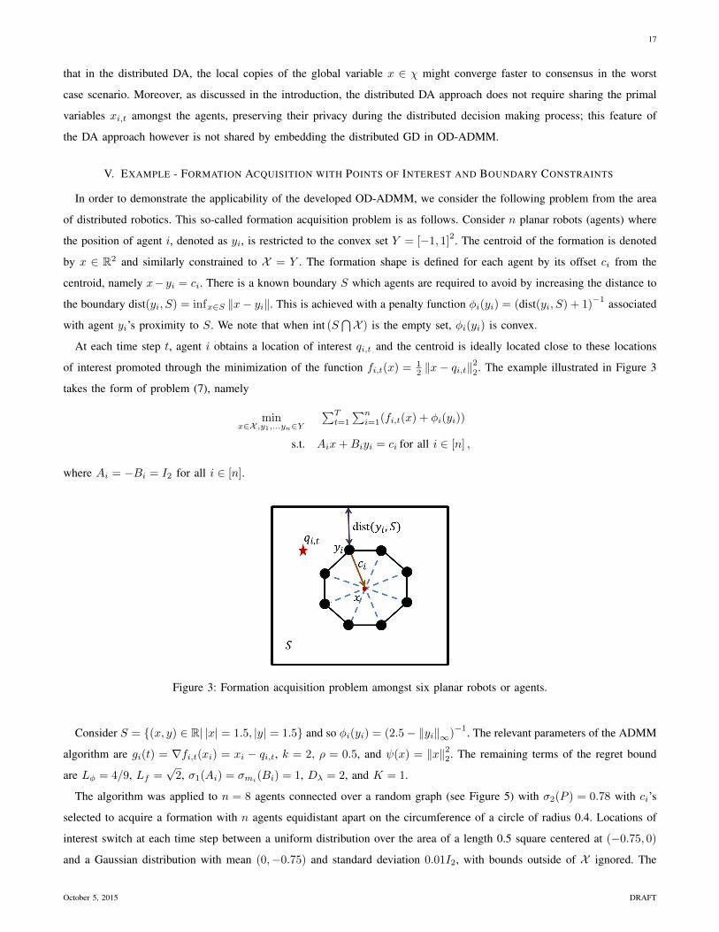
Figure 1: Distributed ADMM problem over a network; each agent operates based of the local objective fi,t(x) +φi(yi) and

the local linear constraint Aix+Biyi = ci.

III. PROBLEM STATEMENT

In this section, we consider a large scale network of agents cooperatively optimizing a global objective function. Let the

communication geometry amongst the n decision-makers or agents, be denoted by the graph G = (V,E). Each node i ∈ V

is an agent that communicates with its neighbor j ∈ N(i) through the edge (i, j) ∈ E. An equivalent online distributed

convex optimization problem to (4) is as follows,

min

x ∈ χ, y1, . . . , yn ∈ Y

T∑t=1

Ft(x, y) :=

T∑t=1

ft(x) +1

n

n∑i=1

φi(yi) (7)

subject to

ri(x, yi) := Aix+Biyi − ci = 0 for all i ∈ [n], (8)

where ft(x) = 1n

∑ni=1 fi,t(x), and fi,t : Rdx → R and φi : Rdy → R are convex for each i. The matrices in the local linear

constraints are denoted as Ai ∈ Rmi×dx , Bi ∈ Rmi×dy , and ci ∈ Rmi at node i ∈ [n] . We assume that BTi is left invertible,

i.e., σmi(BiBTi ) is non-zero, for all i ∈ [n]. The functions fi,t and φi are further assumed to be Lipschitz continuous with

Lipschitz constants Lf and Lφ, respectively, that is,

|fi,t(u)− fi,t(v)| ≤ Lf‖u− v‖ for all u, v ∈ χ,

|φi(u′)− φi(v′)| ≤ Lφ‖u′ − v′‖ for all u′, v′ ∈ Y.

The distributed nature of the optimization is illustrated in Figure 1. assume that the Slater condition holds, namely that there

exists (x, y1, · · · , yn) in the interior of χ× Y . . .× Y that (8) is satisfied. This assumption is naturally used in the analysis

of the duality gap for deriving bounds on the social regret. Moreover, we assume that the set of optimal solutions of (7)

nonempty and the finite optimum value is P∗. diameter of the set χ, defined as diam(χ) = supx,x′∈χ ||x− x′||, is assumed

to be finite and denoted by Dχ.

The local decisions made by agent i is represented by the optimization variables xi ∈ X and yi ∈ Y ; note that we allow

the agents to have a local (not necessary exact) version of the global variable x, namely xi. In addition, we assume that

October 5, 2015 DRAFT

6

subgradients ∂fi,t(x) can be computed for every x ∈ χ. In the online setting, based on the available local information, each

decision maker i selects a global variable xi,t ∈ χ and local variable yi,t ∈ Y , at time t. The cost fi,t(xi,t) is then revealed

to this agent after its local decision xi,t has been committed to at time t.

A. Regret for Constrained Optimization

We now examine a measure for evaluating the performance of OD-ADMM based on variational inequalities. measure is

inspired by the convergence analysis of Douglas-Rachford ADMM presented in [24].

Consider the Lagrangian for the constrained optimization problem (7) as

LT (x, y, λ) =

T∑t=1

ft(x) +

1

n

n∑i=1

(φi(yi) + 〈λi, ri(x, yi)〉)

, (9)

where x ∈ X and yi ∈ Y , as well as assuming λi ∈ Rmi , for all i ∈ [n]. Then, the Lagrange dual function is defined as

D(λ) = infx∈χ,yi∈Y

LT (x, y, λ), (10)

implying that D(λ) is concave and yields a lower bound on the optimal value of (7) [9]. Hence, the dual function D(λ) is

maximized with respect to the variable λ ∈ Rmi×n,

D∗ = maxλ∈Zn

D(λ) = maxλ∈Zn

LT (x∗, y∗, λ); (11)

we note that Zn ⊆ Rmi×n. Slater condition guarantees zero duality gap and the existence of a dual optimal solution λ∗ ∈ Zn.

When (x∗, y∗1 , · · · , y∗n) ∈ χ×Y n solves the primal problem (7)-(8), the primal and dual optimal vectors form a saddle-point

for the Lagrangian LT [25]. Thus, based on the saddle point theorem, if w∗ = (x∗, y∗1 , · · · , y∗n, λ∗1, · · · , λ∗n) ∈ Ω is a saddle

point for LT , then for all w = (x, y1, · · · , yn, λ1, · · · , λn) ∈ χ× Y n × Rmi×n = Ω, we have

LT (x∗, y∗, λ) ≤ LT (x∗, y∗, λ∗) ≤ LT (x, y, λ∗). (12)

Moreover, the Slater condition implies that the dual optimal set is bounded; hence ‖λ∗i ‖ ≤ Dλ for all i ∈ [n] for some finite

Dλ (see Lemma 3 in [26]). A consequence of inequality (12) is that w =(x, y, λ

)∈ Ω approximately solves the primal

problem with accuracy εPT ≥ 0 if it satisfies,

0 ≤ LT (x, y, λ∗)− LT (x∗, y∗, λ∗) ≤ εPT ,

that is,

0 ≤ LT (x, y, λ∗)− P∗ ≤ εPT . (13)

Based on (10), the inequality (13) can also be referred as dual feasibility. In addition, w =(x, y, λ

)∈ Ω approximately

solves the dual problem with accuracy εDT ≥ 0 if

0 ≤ LT (x∗, y∗, λ∗)− LT (x∗, y∗, λ) ≤ εDT ,

that is,

0 ≤ D∗ −D(λ) ≤ εDT , (14)

October 5, 2015 DRAFT

7

Figure 2: This figure illustrates the duality gap at w = (x, y, λ) ∈ Ω.

which represents the dual sub-optimality. The conditions in (13)-(14) can be combined to represent the duality gap asT∑t=1

f∆t (w, w∗) +

1

n(

n∑i=1

φ∆i (w, w∗) +H∆

i (w, w∗)) ≤ εT .

where

f∆t (w,w∗) = ft(x)− ft(x∗)

φ∆i (w,w∗) = φi(yi)− φi(y∗i )

H∆i (w,w∗) = h∆

1i(w,w∗) + h∆

2i(w,w∗)

h∆1i(w,w

∗) =⟨x− x∗, ATi λ∗i

⟩+ 〈λi − λ∗i ,−ri(x∗, y∗i )〉

h∆2i(w,w

∗) =⟨yi − y∗i , BTi λ∗i

⟩,

and εT = εPT + εDT ≥ 0. This gap is illustrated in Figure 2.

Analogous to the regret definition for O-ADMM algorithm [27], we can consider a sequence of decisions wt, where

wt ∈ Ω for each t, instead of a fixed decision w. Consequently, the sequence wt approximately solves (7) and (8) with

accuracy εT ifT∑t=1

f∆t (wt, w

∗) +1

n

n∑i=1

φ∆i (wt, w

∗) +H∆i (wt, w

∗)

≤ εT , (15)

for the optimal solution w∗ ∈ Ω, referred to as fixed case solutions to distinguish them from the time-varying online solution

sequence wt. Moreover, the mapping H∆i (w,w∗) can be expressed as

H∆i (w,w∗) = 〈wi(x)− w∗i (x), Hi(w

∗)〉 ,

where wi(x) =[x yi λi

]T, w∗i (x) =

[x y∗i λ∗i

]T, and

Hi(w) =

0 0 ATi

0 0 BTi

−Ai −Bi 0

wi(x) +

0

0

ci

.

October 5, 2015 DRAFT

8

Since, the mapping Hi(w) is affine in wi(x) and is defined through a skew symmetric matrix, it is monotone, and consequently

[28]

〈wi(x)− w∗i (x), Hi(w)−Hi(w∗)〉 ≥ 0

〈wi(x)− w∗i (x), Hi(w)〉 ≥ 〈wi(x)− w∗i (x), Hi(w∗)〉 . (16)

Therefore, the inequalityT∑t=1

f∆t (wt, w

∗) +1

n

n∑i=1

(φ∆i (wt, w

∗) + 〈wi,t(x)− w∗i (x), Hi(wt)〉)≤ εT (17)

is a sufficient condition for (15).

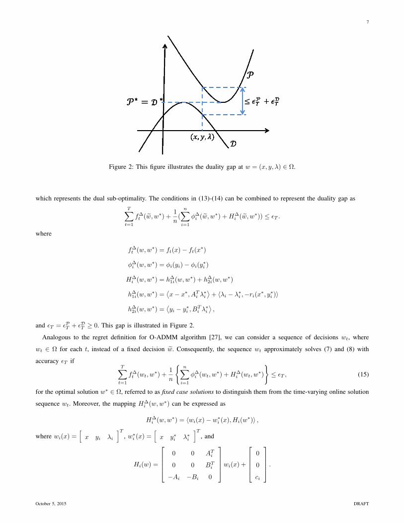
Finally, motivated by the inclusion of regularization terms in the augmented Lagrangian method [25], the term on the left

hand side of (17) is supplemented with terms of the form ρ2 ||ri(xi,t, yi,t)||

2, where ρ > 0, to promote agents satisfy the local

primal feasibility constraints. In our setting, the sequence wi,t is constructed from the distributed algorithm adopted by each

agent i, specifically wt(xi,t) = (xj,t, yt, λt+1) ∈ Ω at time t, where yt = (y1,t, · · · , yn,t) and λt+1 = (λ1,t+1, · · · , λn,t+1).

The social regret is thus defined as,2

RT = maxj∈[n]

Rj,T ,

where

Rj,T =

T∑t=1

f∆t (wt(xj,t), w

∗) +1

n

n∑i=1

φ∆i (wt(xj,t), w

∗) + 〈wi,t(xj,t)− w∗i (xj,t), Hi(wt(xj,t))〉+ρ

2||ri(xi,t, yi,t)||2

.

(18)

Based on (17) we say that the sequence wi,t approximately solves (7) and (8) with accuracy εT if it satisfies RT ≤ εT .

Therefore, if the social regret is sub-linear with time, the online algorithm performs as well as the best fixed case decision

provided with the complete sequence of cost functions a priori. In addition, the sub-linearity of the social regret ensures that

the local linear constraints will be satisfied asymptotically.

IV. MAIN RESULT

The main contribution of this paper is extending O-ADMM [8] via Nesterov’s Dual Averaging (DA) algorithm [29] and

distributed subgradients (descent) method discussed in [13], [30], [31], [32], to provide a distributed decision-making process

for the optimization problem discussed in §III with a sub-linear social regret; we refer to this procedure as online distributed

ADMM (OD-ADMM). The main challenge for the seamless integration of ADMM with dual averaging and distributed

gradient descent for OD-ADMM is deriving and utilizing bounds on the network effect and the sub-optimality of the local

decisions on the quality of the agent’s decisions on the social regret. This objective is achieved by building on the existing

results reported in [13], [14], [15] regarding the network contribution in distributed optimization, as well as extensions of

results discussed in [7], [8], [1]. basic idea behind our convergence analysis is as follows.3 First, in Lemmas 6 and 7, we

derive the gap between the local decisions and the average decision over the network. Then, we provide the sub-optimality

gap in Lemmas 8 and 9. Finally, building on previous results, bounds on the social regret are presented in Theorems 1 and

2.

2Note that this form of regret penalizes the deviation of each agent’s local copy of the global variable from the best fixed global decision in hindsight.3All referenced lemmas are discussed in the Appendix.

October 5, 2015 DRAFT

9

The proposed algorithm updates the vector (xi, yi, zi, λi) for each agent i ∈ [n] by alternately minimizing the Lagrangian

and augmented Lagrangian. In addition, the Lagrangian is linearized based on network-level update, leading to a subgradient

descent method followed by a projection step onto the constraint set χ. Specifically, in the DA method, we let

zt+1 = zt + gt,

where gt = ∇Lt(xt), followed by

xt+1 =

ψ∏χ

(zt+1, αt) ; (19)

in this case, the parameter αt is a non-increasing sequence of positive functions and∏ψχ(·) is the projection operator onto

χ defined asψ∏χ

(zt+1, αt) ≡ arg minx∈χ

〈zt+1, x〉+

1

αtψ(x)

; (20)

the proximal function ψ(x) : χ → R is continuously differentiable and strongly convex . The inclusion of the proximal

function in the DA method as a regularizer prevents oscillations in the projection step. to be strongly convex with respect

to ‖.‖, ψ ≥ 0, and ψ(0) = 0.

On the other hand, in the subgradient descent (GD) method, the aforementioned steps in DA are replaced by

ht+1 = xt − αtgt,

followed by

xt+1 =∏χ

ht+1 ≡ arg minx∈χ||x− ht+1||. (21)

Finally, the proposed online algorithm minimizes the augmented Lagrangian over y as

yt+1 = arg miny∈Y

Lt(xt+1, y, λt+1) +

ρ

2||r(xt+1, y)||2

,

and update the dual variable λ as4

λt+2 = λt+1 + ρ(Axt+1 +Byt+1 − c).

The distributed algorithm can be considered as an approximate ADMM by an agent i via a convex combination of

information provided by its neighbors N(i). Specifically, the global update step (19) and (21) can be reformulated with

a distributed method. The underlying communication network can be represented compactly as a doubly stochastic matrix

P ∈ Rn×n which preserves the zero structure of the Laplacian matrix L(G). For agents to have access to information

contained in the subgradients gi,t = ∇Li,t(xi,t) there must be information flow amongst the agents; as such, in our

subsequent analysis it will be assumed that the graph G is strongly connected. A method to construct a doubly stochastic

matrix P of the required form from the Laplacian of the network is provided in Proposition 3.

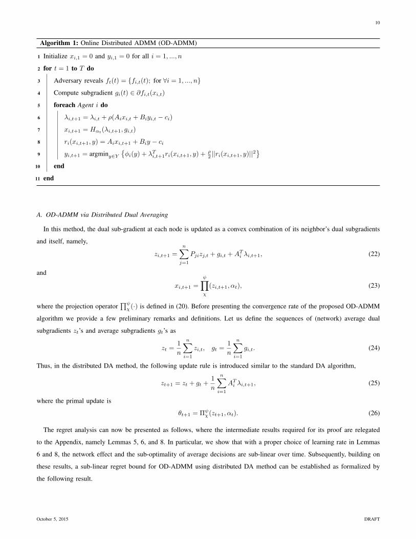
The online distributed ADMM (OD-ADMM) is presented in Algorithm 1.

The function Hαt(λi,t+1, gi,t) referred to on line 8 of the algorithm represents a distributed update on the primal variable.

this paper, we consider two alternatives for this update.

4Note that the index for the dual variable is one time step ahead of the primal variables.

October 5, 2015 DRAFT

10

Algorithm 1: Online Distributed ADMM (OD-ADMM)

1 Initialize xi,1 = 0 and yi,1 = 0 for all i = 1, ..., n

2 for t = 1 to T do

3 Adversary reveals ft(t) = fi,t(t); for ∀i = 1, ..., n

4 Compute subgradient gi(t) ∈ ∂fi,t(xi,t)

5 foreach Agent i do

6 λi,t+1 = λi,t + ρ(Aixi,t +Biyi,t − ci)

7 xi,t+1 = Hαt(λi,t+1, gi,t)

8 ri(xi,t+1, y) = Aixi,t+1 +Biy − ci9 yi,t+1 = argminy∈Y

φi(y) + λTi,t+1ri(xi,t+1, y) + ρ

2 ||ri(xi,t+1, y)||2

10 end

11 end

A. OD-ADMM via Distributed Dual Averaging

In this method, the dual sub-gradient at each node is updated as a convex combination of its neighbor’s dual subgradients

and itself, namely,

zi,t+1 =

n∑j=1

Pjizj,t + gi,t +ATi λi,t+1, (22)

and

xi,t+1 =

ψ∏χ

(zi,t+1, αt), (23)

where the projection operator∏ψχ(·) is defined in (20). Before presenting the convergence rate of the proposed OD-ADMM

algorithm we provide a few preliminary remarks and definitions. Let us define the sequences of (network) average dual

subgradients zt’s and average subgradients gt’s as

zt =1

n

n∑i=1

zi,t, gt =1

n

n∑i=1

gi,t. (24)

Thus, in the distributed DA method, the following update rule is introduced similar to the standard DA algorithm,

zt+1 = zt + gt +1

n

n∑i=1

ATi λi,t+1, (25)

where the primal update is

θt+1 = Πψχ(zt+1, αt). (26)

The regret analysis can now be presented as follows, where the intermediate results required for its proof are relegated

to the Appendix, namely Lemmas 5, 6, and 8. In particular, we show that with a proper choice of learning rate in Lemmas

6 and 8, the network effect and the sub-optimality of average decisions are sub-linear over time. Subsequently, building on

these results, a sub-linear regret bound for OD-ADMM using distributed DA method can be established as formalized by

the following result.

October 5, 2015 DRAFT

11

Theorem 1. Given the sequence wi,t generated by Algorithm 1 where line 7 applies distributed dual-averaging method with

ψ(x∗) ≤ Ψ2 and α(t) = k/√t, we have

RT ≤ J1 + J2k√T , (27)

where

J1 =Dλ

ρn

n∑i=1

ζiσ1(Ai)

,

J2 = 2Q(Lf + ζmax)(2

n

∑i

(Dλσ1(Ai) + 2ζi)),

with

ζ =1

n

n∑i=1

ζi, ζmax = max

iζi,

ζi =√miLφ

σ1(Ai)

σmi(BTi ), and Q =

√n

1− σ2(P ).

Proof: Based on the definition of ft we have

f∆t (wt(xj,t), w

∗) =1

n

n∑i=1

f∆i,t(wt(xj,t), w

∗),

where wt(xj,t) = (xj,t, yt, λt+1) ∈ Ω and thus

Rj,T =1

n

∑i,t

f∆i,t(wt(xj,t), w

∗) + φ∆i (wt(xj,t), w

∗) +H∆i (wt(xj,t), w

∗) +ρ

2||ri(xi,t, yi,t)||2.

In the meantime as ft is L-Lipschitz and convex, we have

f∆t (wt(xj,t), w

∗) = ft(xj,t)− ft(θt) + ft(θt)− ft(x∗)

≤ Lf ‖xj,t − θt‖+ 〈gt, θt − x∗〉 . (28)

The first term in (28) represents the network effect in the regret bound, i.e., the deviation of local primal variable at each

node from the average primal variable. Lemma 6 in the Appendix on the other hand, provides a bound on the network effect

using the DA method. Therefore, replacing line 7 of Algorithm 1 with the distributed DA method implies that

‖θt − xj,t‖ ≤ αt−1

√n (Lf + ζmax)

1− σ2(P ). (29)

Moreover, from the integral test with αt = k/√t it follows that5

T∑t=1

αt−1 ≤ 2k√T . (30)

Hence, from (29) and (30) it follows thatT∑t=1

‖xj,t − θt‖ ≤ 2k√TQ(Lf + ζmax). (31)

5Note that 1√t

is a non increasing positive function and the integral test leads to∑T

t=11√t≤ 2√T − 1.

October 5, 2015 DRAFT

12

The second term in (28) represents the sub-optimality of the procedure due to using the subgradient method. Applying

Lemma 8 (Appendix) with (25) and (26) implies thatT∑t=1

〈gt, θt − x∗〉 ≤T∑t=1

[αt2‖ gt+1 +

1

n

n∑i=1

ATi λi,t+2 ‖2∗

+1

n

n∑i=1

〈λi,t+1, Ai(x∗ − θt)〉] +

1

αTψ (x∗) . (32)

The first term on the the right hand side of (32) represents the sub-optimality of Lagrangian function, defined in (9), with

respect to the global variable x and is bounded as6

T∑t=1

αt2‖ gt+1 +

1

n

n∑i=1

ATi λi,t+2 ‖2∗ ≤ (maxt‖gt+1‖∗ +

1

n

n∑i=1

σ1(Ai) maxt‖λi,t‖∗)

2T∑t=1

αt2. (33)

We now proceed to bound the individual terms in (33). By optimality of line 9 in Algorithm 1 and applying line 6, we

have

∇yφi(yi,t) = −BTi (λi,t + ρri(xi,t, yi,t)) = −BTi λi,t+1,

for all i ∈ [n] and t ∈ [T ]. Moreover, since ||∇yφi(yi,t)|| ≤ Lφ, we have ||BTi λi,t+1|| ≤ Lφ. Thus, λi,t is bounded as

||λi,t|| ≤ ||(BiBTi )−1Bi||F ||BTi λi|| ≤ Lφ(

mi∑j=1

1

σ2j (BTi )

)1/2 ≤√miLφ

σmi(BTi )

, (34)

which implies that ||ATi λi,t|| ≤√miLφσ1(Ai)/σmi

(BTi ). Based on Lipschitz continuity of ft, we have that ‖gt+1‖∗ ≤ Lf ,

and subsequently (33) is bounded asT∑t=1

αt2‖ gt+1 +

1

n

n∑i=1

ATi λi,t+2 ‖2∗ ≤ (Lf + ζ)2k√T . (35)

The second term in the inequality (32) represents the sub-optimality of centralized decision θ with respect to the linear

constraints. In order to analyze this term, it is first expanded into two terms representing the sub-optimality of local decision

xi,t and the network effect, respectively, i.e.,

〈λi,t+1, Ai(x∗ − θt)〉

= 〈λi,t+1, Ai(x∗ − xj,t)〉+ 〈λi,t+1, Ai(xj,t − θt)〉

= 〈λi,t+1, Ai(x∗ − xj,t)〉+ 〈λ∗i − λi,t+1,−ri(xj,t, yi,t)〉

+ 〈λi,t+1, Ai(xj,t − θt)〉+ 〈λ∗i − λi,t+1, ri(xj,t, yi,t)〉

= −h∆1i(wt(xj,t), w

∗) + 〈λi,t+1, Ai(xj,t − θt)〉+ 〈λ∗i − λi,t+1, ri(xj,t, yi,t)〉 . (36)

Based on the network effect introduced in (29), we have

〈λi,t+1, Ai(xj,t − θt)〉 ≤ σ1(Ai)||λi,t+1|| ‖xj,t − θt‖. (37)

Moreover, applying (31) and (34) to (37), it follows thatT∑t=1

〈λi,t+1, Ai(xj,t − θt)〉 ≤ 2k√TζiQ(Lf + ζmax). (38)

6Note that ‖Qx‖ ≤ σ1(Q)||x|| for any matrix Q ∈ Rm×n and vector x ∈ Rn.

October 5, 2015 DRAFT

13

The final term in (36) represents the first order necessary condition for optimality of the dual problem at λi,t+1. By applying

line 7 of the algorithm and an inner product equality, we obtain7

〈λ∗i − λi,t+1, ri(xj,t, yi,t)〉 =1

ρ〈λ∗i − λi,t+1, λi,t+1 − λi,t〉+ 〈λ∗i − λi,t+1, Ai(xj,t − xi,t)〉

=1

2ρ(−‖λi,t+1 − λi,t‖2 + ‖λ∗i − λi,t‖

2 − ‖λ∗i − λi,t+1‖2)

+ 〈λ∗i − λi,t+1, Ai(xj,t − xi,t)〉

=1

2ρ(‖λ∗i − λi,t‖

2 − ‖λ∗i − λi,t+1‖2)− ρ

2‖ri(xi,t, yi,t)‖2

+ 〈λ∗i − λi,t+1, Ai(xj,t − xi,t)〉 . (39)

Resolving the telescoping sumT∑t=1

‖λ∗i − λi,t‖2 − ‖λ∗i − λi,t+1‖2 ,

using the fact λi,1 = 0, it now follows that

T∑t=1

〈λ∗i − λi,t+1, ri(xi,t, yi,t)〉 ≤1

2ρ(‖λ∗i ‖

2 − ‖λ∗i − λi,T+1‖2)− ρ

2

T∑t=1

‖ri(xi,t, yi,t)‖2

≤ 1

2ρ(2 ‖λ∗i ‖ ‖λi,T+1‖)−

ρ

2

T∑t=1

‖ri(xi,t, yi,t)‖2 .

Applying (34) in conjunction with the assumption ‖λ∗i ‖ ≤ Dλ,

T∑t=1

〈λ∗i − λi,t+1, ri(xi,t, yi,t)〉 ≤Dλζiρσ1(Ai)

− ρ

2

T∑t=1

‖ri(xi,t, yi,t)‖2 . (40)

The last term in (39) can also be bounded as

〈λ∗i − λi,t+1, Ai(xj,t − xi,t)〉 ≤ (Dλσ1(Ai) + ζi)‖xj,t − θt‖‖xi,t − θt‖

≤ 2αt−1Q(Lf + ζmax)(Dλσ1(Ai) + ζi) (41)

Substituting (38), (40), and (41) into (36),

1

n

n∑i=1

T∑t=1

〈λi,t+1, Ai (x∗ − θt)〉 ≤ J1 −1

n

∑i,t

h∆

1i(wt(xj,t), w∗) +

ρ

2||ri(xi,t, yi,t)||2

+4k√TQ(Lf + ζmax)(

1

n

n∑i=1

Dλσ1(Ai) + ζ). (42)

Applying ψ (x∗) ≤ Ψ2, αT = k/√T , and substituting (35), (42) into (32) and simplifying, the sub-optimality of the primal

problem at the global decision θt can now be represented asT∑t=1

〈gt, θt − x∗〉 ≤ J1 −1

n

∑i,t

h∆

1i(wt(xj,t), w∗) +

ρ

2||ri(xi,t, yi,t)||2

+k√T × (2Q(Lf + ζmax)(

2

n

∑i

(Dλσ1(Ai) + 2ζi)). (43)

7Namely, using the identity 〈v1 − v2, v3 + v4〉 = 12(||v4 − v2||2 − ||v4 − v1||2 + ||v3 + v1||2 − ||v3 + v2||2.

October 5, 2015 DRAFT

14

Based on our assumption of convexity of φi(·), we have

φ∆i (wi,t, w

∗) ≤ 〈∇yφi(yi,t), yi,t − y∗i 〉

≤ −⟨BTi λi,t+1, yi,t − y∗i

⟩= −h∆

2i(wt(xj,t), w∗). (44)

Combining (43) and (31) into (28) and adding (44), the regret can thereby be bounded as

Rj,T ≤ J1 + J2k√T

for all j ∈ [n] and thus the social regret is bounded as RT ≤ J1 + J2k√T . Note that the social regret represents the worst

case regret amongst the agents in the network.

The above theorem validates the “good” performance of OD-ADMM via dual averaging by demonstrating a sub-linear

social regret. In addition, this social regret highlights the importance of the underlying interaction topology through σ2(P )

and certain condition measure of local linear constraints through σ1(Ai) and σmi(Bi). A well known measure of network

connectivity is the second smallest eigenvalue of the graph Laplacian L(G) denoted by Λ2(G). Since the communication

matrix P is formed as proposed in Proposition 3, 1−σ2(P ) is proportional to Λ2(G) implying that high network connectivity

promotes good performance of the proposed OD-ADMM algorithm with the embedded distributed implementation of dual

averaging.

B. OD-ADMM via Distributed Gradient Descent

In this section, the local primal variable is updated using distributed GD method. In this method xi,t is updated as a

convex combination of its neighbor’s local primal variables and itself, moving in the direction of decreasing the Lagrangian

function,

hi,t+1 =

n∑j=1

Pjixj,t − αt(gi,t +ATi λi,t+1), (45)

followed by the projection onto the convex set χ,

xi,t+1 =∏χ

hi,t+1. (46)

In the distributed GD method, we first define the (network) average primal variable as

θt =1

n

n∑i=1

xi,t. (47)

The regret analysis for the OD-ADMM via the GD method can now be presented as follows, where the intermediate

results required for its proof are relegated to the Appendix, namely Proposition 4, and Lemmas 7 and 9. In particular, with

a proper choice of the learning rate in Lemmas 7 and 9, we can show that the network effect and sub-optimality of the

average decision are sub-linear over time. Then, building on these results, a sub-linear social regret bound for OD-ADMM

using distributed GD method can be obtained; this is formalized in the following theorem.

Theorem 2. Given the sequence wi,t generated by Algorithm 1, where line 7 applies the distributed GD method with

α(t) = k/√t, we have

RT ≤ J1 + J2k√T , (48)

October 5, 2015 DRAFT

15

where

J1 =Dλ

ρn

n∑i=1

ζiσ1(Ai)

+D2χ

2k,

J2 = 4Q(Lf + ζmax)(1

n

n∑i=1

Dλσ1(Ai) + 2ζ) + 2(Lf + ζ)2 + 8LfQ(Lf + ζ),

with

ζ =1

n

n∑i=1

ζi, ζmax = max

iζi,

ζi =√miLφ

σ1(Ai)

σmi(BTi )

, and Q =

√n

1− σ2(P ).

Proof: Based on the definition of ft we have

f∆t (wt(xj,t), w

∗) =1

n

n∑i=1

f∆i,t(wt(xj,t), w

∗),

where wt(xj,t) = (xj,t, yt, λt+1) ∈ Ω and thus

Rj,T =1

n

∑i,t

f∆i,t(wt(xj,t), w

∗) + φ∆i (wt(xj,t), w

∗) +H∆i (wt(xj,t), w

∗) +ρ

2||ri(xi,t, yi,t)||2.

As ft is L-Lipschitz and convex, we have

f∆t (wt(xj,t), w

∗) = ft(xj,t)− ft(θt) + ft(θt)− ft(x∗)

≤ Lf ‖xj,t − θt‖+ 〈gt, θt − x∗〉 . (49)

The first term in (49) represents the network effect in the regret bound, i.e., the deviation of local primal variable at each

node from the average primal variable. In the meantime, Lemmas 6 and 7 in the Appendix provide bounds on the network

effect when the DA and GD methods are used in line 7 of Algorithm 1, respectively. Therefore, replacing line 7 of Algorithm

1 with the distributed DA method implies

‖θt − xj,t‖ ≤ αt−1

√n(Lf + ζmax)

1− σ2(P ), (50)

and with the distributed GD,

‖θt − xj,t‖ ≤ 2√n(Lf + ζmax)

t−1∑k=1

αt−kσ2(P )k−1. (51)

Moreover, from (50) (and (30)) it follows thatT∑t=1

‖xj,t − θt‖ ≤ 4k√T (Q(Lf + ζmax). (52)

Note that the upper bound in (52) is more conservative than the distributed DA method by a factor of 2.

The second term in (49) represents the sub-optimality due to using sub-gradient method. Applying Lemma 9 with (45)-

(47) then leads toT∑t=1

〈gt, θt − x∗〉 ≤2

n2

T∑t=1

αt(

n∑i=1

||gi,t +ATj λi,t+1||)2 +

T∑t=1

(4Lf

t−1∑k=0

αt−kσ2(P )k)1

n

n∑i=1

||(gi,t +ATi λi,t+1||

+1

n

T∑t=1

n∑i=1

⟨ATi λi,t+1, x

∗ − θt⟩

+1

2α1D2χ. (53)

October 5, 2015 DRAFT

16

The first term on the right hand side of (53) is bounded as

2

n2

T∑t=1

αt(

n∑i=1

||gi,t +ATi λi,t+1||)2

≤ 2(1

n

n∑i=1

maxt‖gt+1‖+

1

n

n∑i=1

σ1(Ai) maxt‖λi,t‖)2

T∑t=1

T∑t=1

αt

≤ 2(Lf + ζ)2k√T . (54)

Similarly, the second term on the right hand side of (53) is bounded asT∑t=1

(4Lf

t−1∑k=0

αt−kσ2(P )k)1

n

n∑i=1

||(gi,t +ATi λi,t+1||

≤ 8Lfk√TQ(Lf + ζ). (55)

We now proceed to bound the third term in (53) and from (36) we have

〈λi,t+1, Ai(x∗ − θt)〉 = −h∆

1i(wt(xj,t), w∗) + 〈λi,t+1, Ai(xj,t − θt)〉+ 〈λ∗i − λi,t+1, ri(xj,t, yi,t)〉 . (56)

Analogous to the proof of Theorem 1, the second term of (56) is bounded asT∑t=1

〈λi,t+1, Ai(xj,t − θt)〉 ≤ 4k√TζiQ(Lf + ζmax). (57)

Based on (40) and (41), we haveT∑t=1

〈λ∗i − λi,t+1, ri(xj,t, yi,t)〉 ≤Dλζiρσ1(Ai)

− ρ

2

T∑t=1

‖ri(xi,t, yi,t)‖2 + 4k√TQ(Lf + ζmax)(Dλσ1(Ai) + ζi). (58)

Substituting (57) and (58) into (56),

1

n

n∑i=1

T∑t=1

〈λi,t+1, Ai (x∗ − θt)〉 ≤ −1

n

∑i,t

[h∆1i(wt(xj,t), w

∗) +ρ

2||ri(xi,t, yi,t)||2]

+ 4k√TQ(Lf + ζmax)(

1

n

n∑i=1

Dλσ1(Ai) + 2ζ) +Dλ

ρn

n∑i=1

ζiσ1(Ai)

. (59)

From (54), (55), and (59), the bound on (53) for αt = k/√t is simplified to

T∑t=1

T∑t=1

〈gt, θt − x∗〉 ≤J1 −1

n

∑i,t

[h∆1i(wt(xj,t), w

∗) +ρ

2||ri(xi,t, yi,t)||2]

+ 2k√T (Q(Lf + ζmax)(

2

n

n∑i=1

Dλσ1(Ai) + 4ζ) + (Lf + ζ)2 + 4LfQ(Lf + ζ)). (60)

In the meantime, based on the convexity of φi,

φ∆i (wt, w

∗) ≤ −h∆2i(wt(xj,t), w

∗). (61)

Combining (60) and (52) into (49) and adding (61) we obtain,

Rj,T ≤ J1 + J2k√T .

for all j ∈ [n] and thus RT ≤ J1 + J2k√T .

Theorems 1 and 2 and their proofs provide a basis for comparing two effective methods for evaluating OD-ADMM.

The bounds provided in (31) and (52) for the distributed DA and GD, respectively, although conservative, hint at the fact

October 5, 2015 DRAFT

17

that in the distributed DA, the local copies of the global variable x ∈ χ might converge faster to consensus in the worst

case scenario. Moreover, as discussed in the introduction, the distributed DA approach does not require sharing the primal

variables xi,t amongst the agents, preserving their privacy during the distributed decision making process; this feature of

the DA approach however is not shared by embedding the distributed GD in OD-ADMM.

V. EXAMPLE - FORMATION ACQUISITION WITH POINTS OF INTEREST AND BOUNDARY CONSTRAINTS

In order to demonstrate the applicability of the developed OD-ADMM, we consider the following problem from the area

of distributed robotics. This so-called formation acquisition problem is as follows. Consider n planar robots (agents) where

the position of agent i, denoted as yi, is restricted to the convex set Y = [−1, 1]2. The centroid of the formation is denoted

by x ∈ R2 and similarly constrained to X = Y . The formation shape is defined for each agent by its offset ci from the

centroid, namely x−yi = ci. There is a known boundary S which agents are required to avoid by increasing the distance to

the boundary dist(yi, S) = infx∈S ‖x− yi‖. This is achieved with a penalty function φi(yi) = (dist(yi, S) + 1)−1 associated

with agent yi’s proximity to S. We note that when int (S⋂X ) is the empty set, φi(yi) is convex.

At each time step t, agent i obtains a location of interest qi,t and the centroid is ideally located close to these locations

of interest promoted through the minimization of the function fi,t(x) = 12 ‖x− qi,t‖

22. The example illustrated in Figure 3

takes the form of problem (7), namely

minx∈X ,y1,...yn∈Y

∑Tt=1

∑ni=1(fi,t(x) + φi(yi))

s.t. Aix+Biyi = ci for all i ∈ [n] ,

where Ai = −Bi = I2 for all i ∈ [n].

Figure 3: Formation acquisition problem amongst six planar robots or agents.

Consider S = (x, y) ∈ R| |x| = 1.5, |y| = 1.5 and so φi(yi) = (2.5− ‖yi‖∞)−1. The relevant parameters of the ADMM

algorithm are gi(t) = ∇fi,t(xi) = xi − qi,t, k = 2, ρ = 0.5, and ψ(x) = ‖x‖22. The remaining terms of the regret bound

are Lφ = 4/9, Lf =√

2, σ1(Ai) = σmi(Bi) = 1, Dλ = 2, and K = 1.

The algorithm was applied to n = 8 agents connected over a random graph (see Figure 5) with σ2(P ) = 0.78 with ci’s

selected to acquire a formation with n agents equidistant apart on the circumference of a circle of radius 0.4. Locations of

interest switch at each time step between a uniform distribution over the area of a length 0.5 square centered at (−0.75, 0)

and a Gaussian distribution with mean (0,−0.75) and standard deviation 0.01I2, with bounds outside of X ignored. The

October 5, 2015 DRAFT

18

0.2 0.4 0.6 0.8 1 1.2 1.4 1.6 1.8 2

x 104

10−4

10−3

10−2

10−1

100

Tmax

t∈[T

−t w

,T]g(t)

g(t) = std[xi,t]1g(t) = std[xi,t]2g(t) = 1

n

∑ni=1 ||ri(xi,t,yi,t)||

(a) Distributed Dual Averaging

0.2 0.4 0.6 0.8 1 1.2 1.4 1.6 1.8 2

x 104

10−4

10−3

10−2

10−1

100

T

max

t∈[T

−t w

,T]g(t)

g(t) = std[xi,t]1g(t) = std[xi,t]2g(t) = 1

n

∑ni=1 ||ri(xi,t,yi,t)||

(b) Distributed Gradient Descent

Figure 4: The standard deviation of the global variable xi and the average residue for each agent over times smoothed by

taking the maximum over a tw = 1000 sliding window.

convergence of the global variables xi,t to agreement as well as the reduction of the residue over time are displayed in

Figure 4. Note that the local copies of the global variable converge faster to consensus using the distributed DA as compared

with embedding the distributed GD for OD-ADMM.

The performance of the algorithm was compared for different graph topologies, namely path, star, cycle, random, cube and

complete graphs. These graph topologies are displayed in Figure 5. The matrix P was formed as proposed in Proposition

3, with ε = dmax + 1, as such σ2(P ) = 1 − 1εΛ2(L(G)). Under the same locations of interest as described previously,

the performance of the regret per time RT /T for each graph topology is compared in Figure 6. The performance strongly

correlates with σ2(P ), as predicted in Theorem 2, with smaller σ2(P ) exhibiting improved performance.

VI. CONCLUSION

In this work, online distributed ADMM has been introduced and analyzed, where a network of decision-makers or agents

cooperatively optimize an objective that decomposes to global and local objectives, and is partially online. Moreover, the

local variables and the global variable are linearly constraint (specific to each agent). This problem setup has a wide range

of applications in networked systems, such as in distributed robotics and computer networks. A distributed algorithm allows

October 5, 2015 DRAFT

19

path

star

cycle

random

cube

complete

Figure 5: Topologies of the six different graph types considered for the formation acquisition problem.

Figure 6: The social regret per time RT /T performance of six different graph types, specifically a path, star, cycle, random,

cube and complete graph with σ2(P ) of 0.95, 0.88, 0.80, 0.78, 0.50, 0.00, respectively. The trajectories are smoothed by

taking the average over a tw = 1000 sliding window.

us to make decisions across the network based on local data and information exchange with neighboring agents.

The online distributed algorithm developed in this paper, achieves a sub-linear social regret of O(√T ), that simultaneously

captures sub-optimality of the objective function and the violations in the linear local constraints. In particular, this algorithm

is competitive with respect to the best fixed decision performance in hindsight. Moreover, we have highlighted the role of the

underlying network topology in achieving a “good” social regret, i.e., the regret bound improves with increased connectivity

in the network. The proposed algorithm was then applied to a formation acquisition problem.

Future work of particular interest includes exploring social regret over a time varying network, and investigating favorable

network characteristics for the proposed online distributed ADMM algorithm.

October 5, 2015 DRAFT

20

VII. APPENDIX

The following results can be found in [14], [15], [33]; as such they are presented here with no or abridged proofs.

Proposition 3. If graph G is strongly connected then the matrix P = I − 1ε diag (v)L(G) is doubly stochastic, where

vTL (G) = 0 with positive vector v = [v1, v2, . . . , vn]T and ε ∈ (maxi∈V (vidi),∞). If graph G is balanced then the matrix

P = I − 1εL(G) is doubly stochastic, where ε ∈ (dmax,∞).

Proposition 4. For any u ∈ Rm, v ∈ χ, and orthogonal projection operator∏χ onto χ we have⟨

u−∏χ

(u), u− v

⟩≥ 0.

Lemma 5. For any u, v ∈ Rm, and under the conditions stated for the proximal function ψ and step size α, we have

‖ψ∏χ

(u, α)−ψ∏χ

(v, α)‖ ≤ α‖u− v‖∗.

Lemma 6. For sequences zi,t and xi,t generated by Algorithm 1, using the distributed DA method where,

zi,t+1 =

n∑j=1

Pjizj,t + gi,t +ATi λi,t+1

and xi,t+1 =∏ψχ(zi,t+1, αt), we have

‖θt − xi,t‖∗ ≤ αt−1

√n(Lf + ζmax)

1− σ2(P )

for all i ∈ [n] and t ∈ [T ], where the sequence θt is generated by (26), ζi = Lφσ1(Ai)/σ1(Bi), and ζmax = maxi ζi.

Proof: Based on the definition of zi,t we have

zi,t =

n∑j=1

[P t−1

]jizj,1 +

t−1∑k=1

n∑j=1

[P k−1

]ji

(gj,t−k +ATj λj,t−k+1

).

In addition, zt evolves as

zt = z1 +

t−1∑k=1

n∑j=1

1

n(gj,t−k +ATj λj,t−k+1). (62)

Assuming zi,1 = 0 for all i ∈ [n] and based on (62) we have

zt − zi,t =

t−1∑k=1

n∑j=1

(1

n−[P k−1

]ji

)(gj,t−k +ATj λj,t−k+1) (63)

Thus, the dual norm of zt − zi,t can be bounded as

‖zt − zi,t‖∗ ≤t−1∑k=1

n∑j=1

∥∥gj,t−k +ATj λj,t−k+1

∥∥∗ |

1

n−[P k−1

]ji|

≤t−1∑k=1

maxj

∥∥gj,t−k +ATj λj,t−k+1

∥∥∗ ‖P

k−1ei −1

n‖1. (64)

Since ‖gi,t‖∗ ≤ Lf and ||ATi λi,t||∗ ≤ ζi ≤ ζmax, the dual norm of zt − zi,t is further bounded as 8

‖zt − zi,t‖∗ ≤√n(Lf + ζmax)

t−1∑k=1

σ2(P )k−1. (65)

8Note that ‖P tx − 1n‖1 ≤ σ2(P )t

√n, where the vector x belongs to x ∈ Rn|x ≥ 0,

∑ni=1 xi = 1; this property of stochastic matrices was

similarly used by Duchi et al. [14].

October 5, 2015 DRAFT

21

In addition, as P is a doubly stochastic matrix, σ2(P ) ≤ 1 [34]. Thus, the inequality (65) is bounded as

‖zt − zi,t‖∗ ≤√n(Lf + ζmax)

1− σ2(P ),

Since θt =∏ψχ(zt, αt−1) and xi,t =

∏ψχ(zi,t, αt−1), the statement of the lemma follows from Lemma 5.

Lemma 7. For sequences xi,t and hi,t generated by Algorithm 1 using distributed GD method, where

hi,t =

n∑j=1

Pjixj,t−1 − αt−1(gi,t−1 +ATi λi,t)

and xi,t =∏χ hi,t, we have

‖θt − xi,t‖ ≤ 2√n(Lf + ζmax)

t−1∑k=1

αt−kσ2(P )k−1

for all i ∈ [n] and t ∈ [T ], where the sequence θt is generated by

θt =1

n

n∑i=1

xi,t,

ζi = Lφσ1(Ai)/σ1(Bi), and ζmax = maxi ζi.

Proof: Denote ri,t = xi,t − hi,t; thus based on the definition of hi,t we have

xi,t = hi,t + ri,t =

n∑j=1

Pjixj,t−1 − αt−1(gi,t−1 +ATi λi,t) + ri,t (66)

Subsequently, we can represent xi,t as

xi,t =

n∑j=1

[P t−1

]jixj,1 −

t−1∑k=1

n∑j=1

[P k−1

]ji

(αt−k(gj,t−k +ATj λj,t−k+1

)− rj,t−k+1).

In addition, based on (66), the average primal variable θt evolves as

θt = θ1 −t−1∑k=1

n∑j=1

1

n(αt−k(gj,t−k +ATj λj,t−k+1)− rj,t−k+1). (67)

Assuming xi,1 = 0 for all i ∈ [n] and based on (67), we can represent the network effect, that is the difference between the

average primal variable over the network and individual primal variables, as

θt − xi,t =t−1∑k=1

n∑j=1

(1

n−[P k−1

]ji

)(rj,t−k+1 − αt−k(gj,t−k +ATj λj,t−k+1)). (68)

Thus, the network effect (68) can be bounded as

‖θt − xi,t‖ ≤t−1∑k=1

n∑j=1

∥∥rj,t−k+1 − αt−k(gj,t−k +ATj λj,t−k+1)∥∥ | 1n−[P k−1

]ji|

≤t−2∑k=1

maxj

∥∥rj,t−k+1 − αt−k(gj,t−k +ATj λj,t−k+1)∥∥ ‖P k−1ei −

1

n1‖1 (69)

Moreover, the difference between hi,t and its projection onto χ is bounded as

||ri,t|| = ||∏χ

hi,t − hi,t|| ≤ ||n∑j=1

Pjixj,t−1 − hi,t||

≤ αt−1||gi,t−1 +ATi λi,t||.

October 5, 2015 DRAFT

22

Since ‖gi,t‖∗ ≤ Lf and ||ATi λi,t|| ≤ ζi ≤ ζmax, the network effect is further bounded as

‖θt − xi,t‖ ≤ 2√n(Lf + ζmax)

t−1∑k=1

αt−kσ2(P )k−1. (70)

Lemma 8. For any positive and non-increasing sequence α(t) and x∗ ∈ χT∑t=1

〈gt, θt − x∗〉 ≤T∑t=1

1

n

n∑i=1

⟨ATi λi,t+1, x

∗ − θt⟩

+1

αTψ(x∗) +

T∑t=2

αt−1

2||gt +

1

n

n∑i=1

ATi λi,t+1||2∗,

where the sequence θt is generated by (25)-(26).

Proof: Based on Lemma 3 in [14], we haveT∑t=1

⟨gt +

1

n

n∑i=1

ATi λi,t+1, θt − x∗⟩≤ 1

αTψ(x∗) +

T∑t=2

αt−1

2||gt +

1

n

n∑i=1

ATi λi,t+1||2∗,

and the statement of the lemma follows.

Lemma 9. For any positive and non-increasing sequence α(t) and x∗ ∈ χT∑t=1

〈gt, θt − x∗〉 ≤1

n

T∑t=1

n∑j=1

⟨ATj λj,t+1, x

∗ − θt⟩

+2

n2

T∑t=1

αt(

n∑j=1

||gj,t +ATj λj,t+1||)2

+1

2α1D2χ +

T∑t=1

(4Lf

t−1∑k=0

αt−kσ2(P )k)1

n

n∑j=1

||(gj,t +ATj λj,t+1||,

where the sequence of θt is generated by (45), (46), and (47).

Proof: Denote ri,t = xi,t − hi,t; thus based on the definition of hi,t, we have

xi,t+1 = hi,t+1 + ri,t+1

=

n∑j=1

Pjixj,t − αt(gi,t +ATi λi,t+1) + ri,t+1. (71)

Subsequently, based on (47), the average primal variable θt evolves as

θt+1 = θt −1

n

n∑j=1

(αt(gj,t +ATj λj,t+1)− rj,t+1). (72)

Now, we can represent the deviation of average primal variable θt from x∗ as

||θt+1 − x∗||2 =||θt − x∗||2 +1

n2||

n∑j=1

(αt(gj,t +ATj λj,t+1)− rj,t+1)||2

− 2αtn

n∑j=1

⟨(gj,t +ATj λj,t+1), θt − x∗

⟩+

2

n

n∑j=1

〈rj,t+1, θt − x∗〉 . (73)

Note that

||n∑j=1

(αt(gj,t +ATj λj,t+1)− rj,t+1)||2 ≤

n∑j=1

||αt(gj,t +ATj λj,t+1||+ ||rj,t+1||

2

≤ 4α2t (

n∑j=1

||gj,t +ATj λj,t+1||)2,

October 5, 2015 DRAFT

23

and from Proposition 4 we have

〈rj,t+1, θt − x∗〉 ≤ 〈rj,t+1, θt − hj,t+1〉+

⟨∏χ

hj,t+1 − hj,t+1, hj,t+1 − x∗⟩

≤ 〈rj,t+1, θt − hj,t+1〉 ≤ αt||(gj,t +ATj λj,t+1||||θt − hj,t+1||.

Based on Lemma 8 in [13], we have

〈rj,t+1, θt − x∗〉 ≤ 4Lfαt||(gj,t +ATj λj,t+1||t−1∑k=0

αt−kσ2(P )k.

Thus, by rearranging the terms in (73), we haveT∑t=1

〈gt, θt − x∗〉 ≤1

2α1||θ1 − x∗||2 −

1

2αT+1||θT+1 − x∗||2 +

2

n2

T∑t=1

αt(

n∑j=1

||gj,t +ATj λj,t+1||)2

+1

n

T∑t=1

n∑j=1

⟨ATj λj,t+1, x

∗ − θt⟩

+

T∑t=1

(4Lf

t−1∑k=0

αt−kσ2(P )k)1

n

n∑j=1

||(gj,t +ATj λj,t+1||. (74)

Since the diameter of χ is bounded by Dχ, we have ||θ1 − x∗||2 ≤ D2χ and the statement of the lemma follows.

REFERENCES

[1] S. Hosseini, A. Chapman, and M. Mesbahi, “Online distributed ADMM via dual averaging,” in IEEE Conference on Decision and Control, 2014,

pp. 904–909.

[2] I. Necoara, V. Nedelcu, and I. Dumitrache, “Parallel and distributed optimization methods for estimation and control in networks,” Journal of Process

Control, vol. 21, no. 5, pp. 756 – 766, 2011.

[3] A. Dominguez Garcia, S. Cady, and C. Hadjicostis, “Decentralized optimal dispatch of distributed energy resources,” in IEEE Conference on Decision

and Control, 2012, pp. 3688–3693.

[4] P. Lions and B. Mercier, “Splitting algorithms for the sum of two nonlinear operators,” SIAM Journal on Numerical Analysis, vol. 16, no. 6, pp.

964–979, 1979.

[5] M. Zinkevich, “Online convex programming and generalized infinitesimal gradient ascent,” in International Conference on Machine Learning, 2003,

pp. 421–422.

[6] H. Ouyang, N. He, and A. Gray, “Stochastic ADMM for nonsmooth optimization,” arXiv preprint arXiv:1211.0632, pp. 1–11, 2012.

[7] H. Wang and A. Banerjee, “Online alternating direction method,” in International Conference on Machine Learning, no. 1, 2012, pp. 1119–1126.

[8] T. Suzuki, “Dual averaging and proximal gradient descent for online alternating direction multiplier method,” in International Conference on Machine

Learning, vol. 28, 2013, pp. 392–400.

[9] S. Boyd, “Distributed optimization and statistical learning via the alternating direction method of multipliers,” Foundations and Trends in Machine

Learning, vol. 3, no. 1, pp. 1–122, 2010.

[10] E. Wei and A. Ozdaglar, “Distributed alternating direction method of multipliers,” in IEEE Conference on Decision and Control, 2012, pp. 5445–5450.

[11] F. Iutzeler and P. Bianchi, “Asynchronous distributed optimization using a randomized alternating direction method of multipliers,” in IEEE Conference

on Decision and Control, 2013, pp. 3671–3676.

[12] E. Wei and A. Ozdaglar, “On the O(1/k) convergence of asynchronous distributed alternating direction method of multipliers,” in IEEE Global

Conference on Signal and Information Processing, 2013, pp. 551–554.

[13] F. Yan, S. Sundaram, S. V. N. Vishwanathan, and Y. Qi, “Distributed autonomous online learning: Regrets and intrinsic privacy-preserving properties,”

IEEE Transactions on Knowledge and Data Engineering, vol. 25, pp. 1041–4347, 2013.

[14] J. C. Duchi, A. Agarwal, and M. J. Wainwright, “Dual averaging for distributed optimization: convergence analysis and network scaling,” IEEE

Transactions on Automatic Control, vol. 57, no. 3, pp. 592–606, 2012.

[15] S. Hosseini, A. Chapman, and M. Mesbahi, “Online distributed optimization via dual averaging,” in IEEE Conference on Decision and Control, 2013,

pp. 1484–1489.

[16] A. Koppel, F. Jakubiec, and A. Ribeiro, “A saddle point algorithm for networked online convex optimization,” in IEEE International Conference on

Acoustics, Speech and Signal Processing, 2014, pp. 8292–8296.

October 5, 2015 DRAFT

24

[17] A. G. G. B. Schizas, Ioannis D. Ribeiro, “Consensus in ad hoc WSNs with noisy links - Part I: Distributed estimation of deterministic signals,” IEEE

Transactions on Signal Processing, vol. 56, pp. 350–364, 2008.

[18] J. Mota, J. Xavier, P. Aguiar, and M. Puschel, “D-ADMM: A communication-efficient distributed algorithm for separable optimization,” IEEE

Transactions on Signal Processing, vol. 61, no. 10, pp. 2718–2723, 2013.

[19] W. Deng, M. Lai, and W. Yin, “On the O(1/k) convergence and parallelization of the alternating direction method of multipliers,” arXiv preprint

arXiv:1312.3040, pp. 1–23, 2013.

[20] S. Shalev-Shwartz, “Online learning and online convex optimization,” Foundations and Trends in Machine Learning, vol. 4, pp. 107–194, 2012.

[21] S. Bubeck, “Introduction to online optimization,” Lecture Notes, 2011.

[22] E. Hazan, The Convex Optimization Approach to Regret Minimization. MIT Press, 2012, ch. 10, pp. 287–294.

[23] E. Hazan, A. Agarwal, and S. Kale, “Logarithmic regret algorithms for online convex optimization,” Machine Learning, vol. 69, pp. 169–192, 2007.

[24] B. He and X. Yuan, “On the O(1/n) Convergence Rate of the Douglas-Rachford Alternating Direction Method,” SIAM Journal on Numerical

Analysis, vol. 50, no. 2, pp. 700–709, 2012.

[25] D. Bertsekas, Nonlinear programming. Athena Scientific, 1999.

[26] A. Nedic and A. Ozdaglar, “Subgradient methods for saddle-point problems,” Journal of Optimization Theory and Applications, vol. 142, no. 1, pp.

205–228, 2009.

[27] T. Suzuki, “Stochastic dual coordinate ascent with alternating direction multiplier method,” in International Conference on Machine Learning, 2014,

pp. 736–744.

[28] F. Facchinei and J.-S. Pang, Finite-dimensional variational inequalities and complementarity problems. Springer New York, 2003, vol. 1.

[29] Y. Nesterov, “Primal-dual subgradient methods for convex problems,” Mathematical Programming, vol. 120, no. 1, pp. 221–259, 2007.

[30] A. Nedic and A. Ozdaglar, “Distributed subgradient methods for multi-agent optimization,” IEEE Transactions on Automatic Control, vol. 54, pp.

48–61, 2009.

[31] S. Sundhar Ram, A. Nedic, and V. V. Veeravalli, “Distributed stochastic subgradient projection algorithms for convex optimization,” Journal of

Optimization Theory and Applications, vol. 147, no. 3, pp. 516–545, 2010.

[32] I. Lobel and A. Ozdaglar, “Distributed subgradient methods for convex optimization over random networks,” IEEE Transactions on Automatic Control,

pp. 1291–1306, 2011.

[33] D. Bertsekas, “Incremental proximal methods for large scale convex optimization,” Mathematical Programming, vol. 129, no. 2, pp. 163–195, 2011.

[34] A. Berman and R. J. Plemmons, Nonnegative Matrices in the Mathematical Sciences. Academic Press, 1979.

October 5, 2015 DRAFT