Salihu Mohammed - University of Ghana

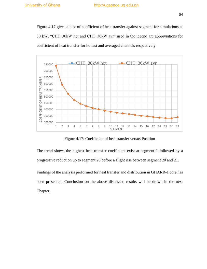
i

Investigation of Heat Transfer and Distribution in the Core of Ghana

Research Reactor-1 (GHARR-1) using STAR-CCM+ CFD Code

Salihu Mohammed

DEPARTMENT OF NUCLEAR ENGINEERING GRADUATE SCHOOL OF

NUCLEAR AND ALLIED SCIENCES COLLEGE OF BASIC AND APPLIED

SCIENCES UNIVERSITY OF GHANA

M.Phil

July, 2015

University of Ghana http://ugspace.ug.edu.gh

ii

Investigation of Heat Transfer and Distribution in the core of Ghana

Research Reactor-1 (GHARR-1) using STAR-CCM+ CFD Code

This thesis is submitted to the:

Department of NUCLEAR ENGINNERING COLLEGE OF BASIC AND APPLIED

SCIENCES, UNIVERSITY OF GHANA

By

(Salihu Mohammed, 10391561)

BSc (Nigeria), 2005

In partial fulfilment of the requirements for the award of the degree of

MASTER OF PHILOSOPHY

In

NUCLEAR ENGINEERING

July, 2015


iii

DECLARATION

This thesis is the result of work undertaken by Salihu Mohammed towards the award of

Master of Philosophy in the Department of Nuclear Engineering, School of Nuclear and

Allied Sciences, University of Ghana, under the Supervision of Dr. Vincent Yao

Agbodemegbe and Dr. S. K. Debrah.

_ _ _ _ _ _ _ _ _ _ _ _ _ _ _ _

Salihu Mohammed

Date:

_ _ _ _ _ _ _ _ _ _ _ _ _ _ _ _ _ _ _ _ _ _ _ _ _ _ _ _ _ _ _ _ _ _

Vincent Yao Agbodemegbe, Ph.D. Seth Kofi Debrah, Ph.D.

(Principal Supervisor) (Co-Supervisor)

Date: Date:


iv

DEDICATION

To my truest love; Salmah Salihu Mohammed, Her Aunty; Talatu Salihu Galadima and

her Grandmother; Ummulkhair Salihu Galadima.


v

ACKNOWLEDGEMENTS

First, I acknowledge Allah (S.W.T) for seeing me through the numerous hurdles that

characterized my academic pursuit. I acknowledge the contributions of my supervisors Dr.

S. K. Debrah and Dr. Vincent Yao Agbodemegbe. I also wish to specially acknowledge

Emeritus Prof. E.H.K. Akaho and Dr. Emmanuel Ampomah-Amoako for their guidance

throughout the programme. My acknowledgement also goes to the Staff of Nuclear

Engineering Department, School of Nuclear and Allied Sciences (SNAS), Staff of Ghana

Atomic Energy Commission (GAEC) especially Ghana Research Reactor-1 (GHARR-1)

facility Engineer, Mr. Edward Oscar Amponsah-Abu, my friends and housemates at SNAS

hostel especially Francis Siaw Nkansah and Lucky Woko for providing a power back-up

used for the research simulations.

I wish to express my profound gratitude to the Chairperson, Niger State Polytechnic Board

of Governing Council -Hajiya Dije Bala for helping me in getting the initial funding for

this programme. I also owe a special acknowledgement to the sitting Rector of the

Polytechnic at the time of my release for this study; Dr. Garba Kamaye Mohammed, the

then Head of Basic and Applied Sciences Department; Late Mal. A. U. Abdulrashid. I also

acknowledge my dear brother Adamu Salihu Rijau for always been there for me as a

brother and a friend throughout my stay in Ghana. Garba Attah, Jamilu Umar Babuga,

Aisha Mohammed Garo, Fatima Ogah, Tukur Mohammed Basey, Awwal Ibrahim

Wushishi, Mal. Yahaya Zakari and Mal. Kasim I. Mohammed are also acknowledged.

I am also indebted to the following Organizations; Niger State Polytechnic, SNAS

University of Ghana, Ghana Atomic Energy Commission, Rijau LGA Community and

Developers of STAR-CCM+ (CD-ADAPCO).


vi

TABLE OF CONTENTS

Declaration i

Dedication ii

Acknowledgements iii

Table of Contents iv

List of Tables vii

List of Figures viii

Nomenclature x

Abstract 1

CHAPTER 1: INTRODUCTION 2

1. Background 2

1.1 Description of Ghana Research Reactor-1 (GHARR-1) 2

1.1.1 Natural Convection 5

1.1.2 GHARR-1 Thermal Hydraulic Associated With heat Removal 6

1.1.3 GHARR-1 Heat Transfer Distribution 7

1.2 Problem Statement 8

1.3 Justification for Research 8

1.4 Research Objectives 9

1.5 Scope of Research 10

1.6 Organization of Thesis 10


vii

CHAPTER 2: LITERATURE REVIEW 11

2.1 Introduction 11

2.2 Computational Fluid Dynamic Tool – STAR-CCM+ 11

2.2.1 STAR-CCM+ Models 14

2.2.1.1 Physics Models 14

2.2.1.2 Continuity Equation 14

2.2.1.3 Momentum Equations 14

2.2.1.4 Energy Equation 15

2.2.1.5 K-Epsilon Turbulence Models 15

2.2.1.6 Wall Y+ 16

2.2.1.7 Segregated Flow Model 16

2.2.1.8 Three-Dimensional Model 17

2.3 Thermal Hydraulic Studies 17

2.4 Heat Transfer and Distribution Parameters 20

CHAPTER 3: METHODOLOGY

3.1 Experimental 22

3.2 STAR-CCM+ Simulation 24

3.2.1 Geometry Modelling 24

3.2.2 Mesh Generation 25

3.2.3 Setting-up Physics 26

3.3 Power Peaking Factors Calculation 30

3.4 Heat Flux Calculation for the Modified Geometry 31


viii

CHAPTER 4 - RESULTS AND DISCUSSION 32

4.1 Introduction 32

4.2 Validation of Simulation Data 33

4.3 Distribution of Wall Y+ In the Domain 39

4.4 Surface average Temperature 40

4.5 Bulk average Temperature 42

4.6 Surface and Bulk Temperature comparison 44

4.7 Bulk average Turbulent Intensity 46

4.8 Channel Centerline Pressure 48

4.9 Contour Plots for Hottest Channel Simulation at 30 Kw 50

4.10 Coefficient of Heat Transfer 52

CHAPTER FIVE -CONCLUSION AND RECOMMENDATION

5.1 Conclusion 55

5.2 Recommendations 56

References 58

Appendix 61


ix

LIST OF TABLES

1.1: Technical Specification for GHARR-1 5

1.2: Physics Specification for GHARR-1 5

3.1: Meshing Models 25

3.2: Physics Model 26

3.3: Power Peaking Factors for GHARR-1 Core 30

4.1: Effect of mass flow rate on outlet temperature at 30 kW 37

4.2: Power level trends for difference for surface average temperature 41

4.3: Mass flow rate and pressure drop for 30 kW power 50


x

LIST OF FIGURES

1.1: GHARR-1 fuel cage showing 344 fuel pins, 4 tie rods, 6 dummy rods, and control

rod 3

1.2: heat transfer mechanism in GHARR-1 4

2.1: STAR-CCM+ User Interface 11

3.1: GHARR-1 core coolant modified geometry 24

3.2: Mesh scene 26

3.3: cylindrical flow channel showing imposed boundary conditions 28

3.4: channel temperature development with time 29

4.1: position of constrained planes in the geometry 32

4.2: position of line probes in the geometry 32

4.3a: Graph of Outlet Temperature versus Power for Hottest Channel 33

4.3b: Graph of Outlet Temperature versus Power for Averaged Channel 34


4.4b: Graph of Outlet Temperature versus Power for Averaged Channel 35


4.5b: Graph of Outlet Temperature versus Power for Averaged 36

4.6: Wall y+ distribution over the domain 39

4.7a: Surface Average Temperature versus Position for Hottest channel 40

4.7b: Surface Average Temperature versus Position for Averaged channel 41

4.8a: Bulk Average Temperature versus Position for Hottest channel 43

4.8b: Bulk Average Temperature versus Position for Averaged channel 43

4.9: Surface and Bulk Temperature for Hottest Channel versus Position for 15kW 44


xi

4.10: Temperature distribution trend 45

4.11a: Bulk Average Turbulent Intensity versus Position for Hottest Channel 47

4.11b: Turbulent Intensity versus Position for Averaged channel 47

4.12a: Fluid Centerline Pressure versus position for hottest channel 49

4.12b: Fluid Centerline Pressure versus position for Averaged channel 49

4.13: Inlet segment temperature distribution 40

4.14: Temperature distribution for segment 21 51

4.15: outlet segment temperature distribution 51

4.16: Surface temperature distribution 52

4.17: Coefficient of heat transfer versus segment 53


xii

NOMENCLATURE

Roman letters

x, y and z direction of coordinates

D dimension (s)

t time

U, V and W momentum components in x, y and z directions

P Pressure

S source term

G productivity buoyancy

A flow area

W Inlet mass flow rate

K turbulent kinetic energy

U, V and W mass flow rates in x, y and z directions

A, B, C…. fuel rod positions

T temperature

D, d diameter

v velocity

G mass flux

Re. Reynold’s

h height

f power peaking factor

Q total power

q segmental power


xiii

Greek Letters

ρ density

ɛ dissipation rate

τ turbulent dissipation time-scale

Ʃ summation

μ dynamic viscosity

ϕ heat flux

Subscripts

x, y, and z direction components

b buoyancy

in inlet

s surface

H hydraulic

ith position number

T total

Abbreviations

STAR-CCM+ Simulation of Turbulent flow in Arbitrary Regions

Computational Continuum Mechanics C++ based

MNSR Miniature Neutron Source Reactors

CFD Computational Fluid Dynamics

CAD Computer-aided Design

CAE Computer-aided Engineering

MATLAB Matrix Laboratory

MAC Marker and cell

COMSOL Computer Solution

TRIGA IPR-R1 Training, Research, Isotopes, General Atomic.


xiv

NIST National Institute of Standards and Technology

Exp. Experimental

Sim. Simulation

Avr. Averaged

Out. Outlet

Temp. Temperature

Hot. Hottest

Tke Turbulent Kinetic Energy

Tdr Turbulent Dissipation Rate

SAT Surface Average Temperature

BAT Bulk Average Temperature

BAD Bulk Average Density

BADV Bulk Average Dynamic Viscosity

BATC Bulk Average Thermal Conductivity

BATKE Bulk Average Turbulent Kinetic Energy

BAV Bulk Average Velocity

Pres. Pressure

No. Number

CHT Coefficient of Heat Transfer

TI Turbulence Intensity


http://www.nist.gov/

1

ABSTRACT

In the present work, STAR-CCM+ CFD code was used to investigate steady state thermal

hydraulic parameters in the core of Ghana Research Reactor-1 (GHARR-1). The core was

segmented into 21 axial segments. 3D-CAD parametric solid modeler embedded in STAR-

CCM+ was used to model the geometry. The geometry was discretized by the use of

appropriate meshing models. GHARR-1 operating conditions were set as boundary

conditions for the STAR-CCM+ simulation conducted. Heat flux specific to individual

axial segment computed based on segment power peaking factors and surface area was

applied at the wall of the flow channel. For each power level, mass flow rate and

temperature were imposed as boundary conditions at the inlet. Standard k-ɛ turbulence

model was adopted for the solution of the transported variables namely turbulent kinetic

energy and its dissipation rate. The results obtained were validated with experimental data

from GHARR-1 operation and observed to be in appreciable agreement. The plots of the

evaluated flow parameters show that the heat applied at the surface of the flow channel is

efficiently transferred to the bulk of the fluid. In addition, effective distribution of

temperature in the domain was observed. With effective heat transfer coupled with uniform

heat distribution, it could be stated that cooling of GHARR-1 fuel which is needed for

safety operation of the facility is assured.


2

CHAPTER 1

INTRODUCTION

This chapter presents the problem statement and provides justification for the research. It

also gives a background for the present study and the scope of work.

1. BACKGROUND

For a normal operation of a nuclear reactor, all the heat released in the system must be

removed very effectively by the coolant. In a nuclear reactor system, liquid or gaseous

coolant pass through the core and through other regions where heat is generated. The

effectiveness of the coolant system is one of the most important considerations in safe

operation and design considerations. For an efficient natural cooling process, it is necessary

to fully understand the mechanism of heat dissipation under different operating conditions

[1].

In the present study, the type of system considered is a single phase flow system as present

in GHARR-1. The cooling process in GHARR-1 is by natural convection.

1.1 DESCRIPTION OF GHANA RESEARCH REACTOR-1 (GHARR-1)

GHARR-1 is a tank-in-pool type, low power research reactor, which is under-moderated

with 10 irradiation sites (5 inside and 5 outside the beryllium annulus reflector) [2, 3].

GHARR-1 uses 90.2 % enriched U-Al alloy as fuel. The diameter of the fuel meat is 4.3

mm and the thickness of the aluminum cladding material is 0.6 mm. The total length of the

element is 248 mm and the active length is 230 mm. The percentage of U in the UAl4

dispersed in Al is 27.5 % and the loading of U-235 in the core with 344 fuel element is

990.72 g [4]


3

The reactor is designed to be compact and safe. It is used mainly for neutron activation

analysis, production of short-lived radioisotopes and for education and training. The

maximum thermal neutron flux at its inner irradiation site is 1×1012 n.cm-2.s-1 . It is cooled

and moderated with light water, and light water and beryllium act as reflectors. The fuel

cage consists of 344 fuel pins, 4 tie and 6 dummy rods, a central control rod guide tube,

upper and lower grid plates as presented in Figure 1.1.

Figure 1.1: GHARR-1 fuel cage showing 344 fuel pins, 4 tie rods, 6 dummy rods and

control rod

The fuel pins, tie and dummy rods are concentrically arranged in 10 rings of the fuel cage.

The core has a central guide tube through which a cadmium control rod cladded in stainless

steel moves to cover the active length of 230 mm of the core. The single control rod is used

for regulation of power, compensation of reactivity and for reactor shutdown during normal

and abnormal operations. The fuel cage is placed on a 50 mm thick beryllium reflector of

diameter 290 mm and it is surrounded by another 100 mm thick metallic beryllium reflector

of height 238.5 mm [4, 5, and 6].


4

The core is cooled by natural convection and under normal operating conditions, the flow

regime is single phase but nucleate boiling is expected under abnormal condition when

power excursion occurs due to large reactivity insertion. There are two pairs of NiCr-NiAl

thermocouples, which are fixed in the inlet and outlet of the core coolant for measuring the

temperature difference between the inlet and the outlet of the coolant. A platinum

resistance thermometer is used for measuring the inlet temperature of the coolant [4, 5, and

6]. The coolant flow in the core is at the transient phase from laminar flow to turbulent

flow. The flow transition will occur when there is an increase in power. The closer to the

upper part of elements, the stronger the turbulence becomes [5]. A diagrammatic

representation of the heat transfer mechanism is presented in Figure 1.2.

Figure 1.2: heat transfer mechanism in GHARR-1 [7]


5

Table 1.1 and Table 1.2 provides the technical and physical specifications for GHARR-1

respectively.

Table 1.1: Technical Specifications for GHARR-1

S/No Geometries Dimensions

1 Core Shape Cylinder

2 Core height 23 cm

3 Core diameter 23 cm

4 Number of fuel elements 344

5 Fuel rod diameter (external) 5.5 mm

6 Fuel rod diameter (external) 4.3 mm

7 Number of dummy rods 6

8 Dummy rod diameter 5.5 mm

9 Number of tie rods 4

10 Tie rod diameter 5.5

11 Total lattice position 356

12 Number of control rods 1

13 Control rod diameter 5 mm

14 Guide tube thickness 3 mm

15 Guide tube diameter 6 mm

16 Number of Segmentation 21

17 Segment Length 10.95 mm

Table 1.2: Physics Specification for GHARR-1

S/No Initial Conditions Magnitude

1 Pressure at inlet 1 bar

2 Flow rate 400L/h (0.111 kg/s)

3 Density of water 999.7 kg/ m3

4 Initial temperature used 307.15 K

5 Power 15 KW

6 Velocity 0.002 m/s

1.1.1 Natural Convection

In GHARR-1, the water in the reactor core is not pressurized and it relies upon natural

convection [8]. Natural Convection Processes are driven by body forces exerted directly

within the fluid as a result of heating or cooling [9]. Natural convection is a mechanism, or


6

type of heat transport, in which the fluid motion is not generated by any external source

(like a pump, fan, suction device, etc.) but only by density differences in the fluid occurring

due to temperature gradients. In natural convection, fluid surrounding a heat source

receives heat, becomes less dense and rises. The surrounding, cooler fluid then moves to

replace it. This cooler fluid is then heated and the process continues, forming a convection

current; this process transfers heat energy from the bottom of the convection cell to top.

The driving force for natural convection is buoyancy, a result of differences in fluid density

[10].

Single phase flow is the flow of a material, as a gas, single-phase liquid, or a solid, but

not in any combination of the three [11]. In GHARR-1 the flow regime is single phase

deionized water.

1.1.2 GHARR-1 thermal hydraulic associated with heat removal

For safety analysis of MNSR’s, a detailed understanding of the reactor heat transfer and

distribution is necessary. The core region of GHARR-1 is located 4.7 m under water close

to the bottom of a watertight reactor vessel. The quantity of water is 1.5 m3 in the vessel,

which serves the purpose of radiation shielding, moderation and as primary heat transfer

medium. In addition, heat can be extracted from the water in the vessel by means of a

water-cooling coil located near the top of the vessel. The water-filled reactor vessel is in

turn immersed in a water-filled pool of 30 m3. Cold water is drawn through the inlet orifice

by natural convection. The water flows past the hot fuel elements and comes out through

the core outlet orifice. The hot water rises to mix with the large volume of water in the

reactor vessel and to the cooling coil. Heat passes through the walls of the container to the


https://en.wikipedia.org/wiki/Heat_transport

https://en.wikipedia.org/wiki/Temperature_gradient

7

pool water. The reactor core is immersed in a large reactor vessel containing deionized

water, which possesses a considerable heat capacity. Even under accident conditions,

removal of heat is by natural circulation to this large heat sink. The core inlet flow orifice

impedes the natural circulation of water through the core. Its area is fixed during assembly

of the reactor and it is deliberately chosen such that the highest power achieved during the

design basis self-limiting power excursion can cause no damage to the core or present any

hazard to staff about the reactor. From thermal-hydraulic tests and calculations, especially

from the transient experiment, it has been found that the reactor has negative feedback

effect. Hence, when the temperature difference between the inlet and outlet coolant of the

reactor increases, the buoyancy and circulating head will increase to make the flow velocity

rise and in turn, limit the increase in power [8].

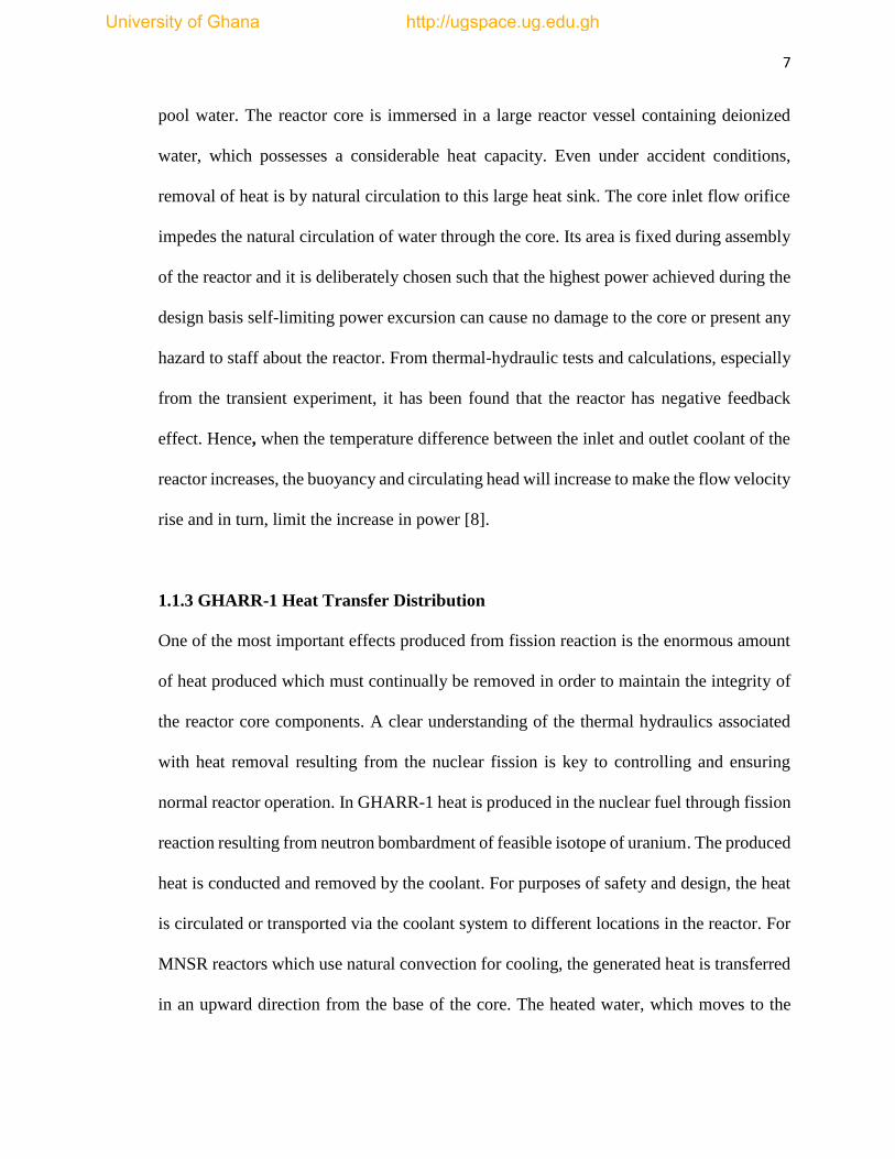
1.1.3 GHARR-1 Heat Transfer Distribution

One of the most important effects produced from fission reaction is the enormous amount

of heat produced which must continually be removed in order to maintain the integrity of

the reactor core components. A clear understanding of the thermal hydraulics associated

with heat removal resulting from the nuclear fission is key to controlling and ensuring

normal reactor operation. In GHARR-1 heat is produced in the nuclear fuel through fission

reaction resulting from neutron bombardment of feasible isotope of uranium. The produced

heat is conducted and removed by the coolant. For purposes of safety and design, the heat

is circulated or transported via the coolant system to different locations in the reactor. For

MNSR reactors which use natural convection for cooling, the generated heat is transferred

in an upward direction from the base of the core. The heated water, which moves to the


8

upper section of the reactor tank, is transferred to the pool water via conduction through

the reactor vessel [7, 8]. The core is cooled by natural convection and under normal

operational conditions, the flow regime is single phase but nucleate boiling is expected

under abnormal condition when power excursion occurs due to large reactivity insertions.

A platinum resistance thermometer is used for measuring the inlet temperature of the

coolant [7].

1.2 PROBLEM STATEMENT

Reactor design and operation is limited by heat transfer consideration and not neutronic

[12]. This is because the reactor core can withstand a neutron flux of any magnitude as

long as the heat generated as a result of the fission reaction can be efficiently removed. It

is on the basis of safety guided by thermal consideration that fuel, coolant and other

structural materials are selected during design.

Previous research [7, 13] conducted on heat transfer for GHARR-1 were performed using

1-D codes namely PARET and PLTEMP thermal hydraulic codes. However, these 1-D

codes do not provide detailed information on the variation of the trends of flow field

parameters at specific locations within the core. The mass flow rate of the coolant at which

effective heat transfer removal from the fuel is obtained is unknown. Also, previous studies

offers no explanation on turbulent intensity of GHARR-1 core coolant.

1.4 JUSTIFICATION FOR RESEARCH

In GHARR-1 core, heat generated in the fuel is removed by natural convection. Ineffective

heat transfer in the reactor core will lead to degradation of the fuel element, reactor vessel,


9

or both. The knowledge of heat transfer and distribution in GHARR-1 will help inform its

safe operation and optimization of the heat transfer processes.

Previous research on GHARR-1 -core heat transfer were done with 1-D generated codes

and results obtained provided limited information. However with the application of the

STAR-CCM+ it is deemed that improved analysis will be conducted to produce more

reliable and detailed results. In addition STAR-CCM+ has the advantage of 3-D

visualization and hence offer improved appreciation of the results.

1.4 RESEARCH OBJECTIVES

The present research aims to analyze heat transfer and distribution in the core of GHARR-

1 using STAR-CCM+ code at different power levels. The specific objectives to be attained

are,

1. To model a simplified GHARR-1 core that mimics the thermal hydraulics of the

full GHARR-1 geometry using 3-D CAD model available in STAR-CCM+.

2. To generate a suitable mesh for the modelled geometry. Using the STAR-CCM+

Code.

3. To select appropriate physics models for the case under study

4. Perform simulation at various reactor power level at a step increase of 5 kW for 5-

30 kW.

5. Analyse the generated data for steady state thermal-hydraulic performance of

GHARR-1.


10

1.5 SCOPE OF RESEARCH

In the present work, STAR-CCM+ Code is used to analyze thermal hydraulic parameters

of a simplified GHARR-1 core for the range 5-30 kW power levels. The work is limited to

a steady state single phase flow without kinetics considerations.

This research is reported in five chapters. The next section discusses the outline of write-

up presentation.

1.6 ORGANIZATION OF THESIS

Chapter 2 discusses general review of literature on heat transfer for research reactors with

emphasis on low power research reactors of the MNSR type. And it also provides a review

of the Reynolds Average Navier Stoke’s (RANS) turbulence model used in STAR-CCM+

code. In Chapter 3, the method of solution and experimental procedure are presented.

Chapter 4 provides validation of the simulated results and discusses result of the research

findings. Chapter 5 is the concluding chapter where conclusions and deductions are made

for each of the results discussed in chapter 4. This chapter also presents suggestion for

possible areas of further studies.

In this chapter the research problem has been stated and justified and a background of the

study provided. The next chapter presents review of related literature for the current study.

It also provides some review on the capabilities of STAR-CCM+ used for the simulation.


11

CHAPTER 2

LITERATURE REVIEW

The present chapter presents review of related literature for the present study. It also

provides some review on the capabilities of STAR-CCM+ CFD code used for the

simulation.

2.1 INTRODUCTION

Interest in safety issues of nuclear research reactors is increasing due to increased

application of neutrons for several types of scientific and social purposes in addition to

power generation. To ensure safe utilization of such installations several codes have been

used with special attention to research reactors. A combination of codes for thermal

hydraulic analysis, for assessment of probabilistic risk, fuel investigation and reactor

physics studies are fundamental tools for an appropriate reactor behavior definition [14].

Research reactor types include Siemens Unterrichtsreaktor, Argonaut reactor, Slowpoke

reactor, the miniature neutron source reactor, TRIGA reactors, Material testing reactors

and High flux reactors [15]. One of such codes used in nuclear industries is the STAR-

CCM+ CFD code which is employed for the present study. The features of this code are

presented in section 2.2.

2.2 COMPUTATIONAL FLUID DYNAMIC (CFD) TOOL

CFD codes comprise of pre-processor, solver and post-processor phases. The

preprocessing is concerned with the geometry modelling, definition of material properties,

mesh generation and physics definition [16]. The CFD codes solver section deals with the


12

solver type specification and analysis runs. It solves the transport equations on every node

defined during the mesh generation step and any additional models specified in the physics

set up [17]. For post processing, CFD codes allow for setting different plots and scenes

either before, during or after running the simulation. These plots and scenes are then

analyzed on attainment of convergence of the solution.

For the present work, STAR-CCM+ CFD code is considered for investigation of heat

transfer and distribution. STAR-CCM+ is a comprehensive engineering simulation tool

used to solve problems involving fluid flow, heat transfer, condensation and stability

analysis just to mention a few [18]. STAR-CCM+ is a CFD code structured around

numerical algorithms that can tackle fluid flow problems accounting for turbulence effects

[19, 20] as it employs the Finite Volume Approach to address a wide variety of modeling

needs. STAR-CCM+ is equipped with the following;

• 3D-CAD modeler

• Surface preparation tools

• Automatic meshing technology

• Physics modeling options

• Turbulence modeling options

• Post-processing and monitors

The object-oriented nature of STAR-CCM+ code can be seen in the user interface

presented in Figure 2.1.


13

Figure 2.1: STAR-CCM+ user Interface

Geometry window allows for modeling of studied dimensions using the 3D-CAD within

STAR-CCM+. This also allows for exporting geometry from 3D-CAD and ascending the

modelled geometry in the simulation. Continua window is concerned with physics and the

mesh continuum. This allows the user to input the properties of materials and also give the

properties of the mesh. It also allow users to specify boundary conditions to be imposed on

various parts. Solvers window works with chosen meshing and physics models to attain

solutions and communicate them to the user. The user-specified models provide the

required transport equations to be solved by the solver. Derived parts window allow user

to set up probes and constraint planes at any point within or outside the geometry. The

available windows are used to specify model properties by utilizing the STAR-CCM+

models described in section 2.2.1.


14

2.2.1 STAR-CCM+ Models

2.2.1.1 Physics Models

The governing equations used for command execution by STAR-CCM+ solver are the

conservation of mass, momentum and the energy equations given in equations 2.1 to 2.5.

2.2.1.2 Continuity Equation

𝜕𝜌

𝜕𝑡+

𝜕(𝜌𝑢)

𝜕𝑥+

𝜕(𝜌𝑣)

𝜕𝑦+

𝜕(𝜌𝑤)

𝜕𝑧= 0 (2.1)

where ρ is the density, t is time (s), x, y and z are components of momentum in x, y and z

planes respectively, u, v and w are components of velocity corresponding to x, y and z

planes respectively.

2.2.1.3 Momentum Equations

U- Momentum

𝜕(𝜌𝑈)

𝜕𝑡+

𝜕

𝜕𝑥(𝜌𝑈2 − 𝜇𝑒

𝜕𝑈

𝜕𝑥) +

𝜕

𝜕𝑦(𝜌𝑈𝑉 − 𝜇𝑒

𝜕𝑈

𝜕𝑦) +

𝜕

𝜕𝑧(𝜌𝑈𝑊 − 𝜇𝑒

𝜕𝑈

𝜕𝑧) = −

𝜕𝑝

𝜕𝑥+ 𝜌𝑔𝑥 (2.2)

V- Momentum

𝜕(𝜌𝑈)

𝜕𝑡+

𝜕

𝜕𝑥(𝜌𝑈𝑉 − 𝜇𝑒

𝜕𝑈

𝜕𝑥) +

𝜕

𝜕𝑦(𝜌𝑉2 − 𝜇𝑒

𝜕𝑈

𝜕𝑦) +

𝜕

𝜕𝑧(𝜌𝑉𝑊 − 𝜇𝑒

𝜕𝑉

𝜕𝑧) = −

𝜕𝑝

𝜕𝑦+ 𝜌𝑔𝑦 (2.3)

W-Momentum

𝜕(𝜌𝑊)

𝜕𝑡+

𝜕

𝜕𝑥(𝜌𝑈𝑊 − 𝜇𝑒

𝜕𝑊

𝜕𝑥) +

𝜕

𝜕𝑦(𝜌𝑉𝑊 − 𝜇𝑒

𝜕𝑊

𝜕𝑦) +

𝜕

𝜕𝑧(𝜌𝑊2 − 𝜇𝑒

𝜕𝑊

𝜕𝑧) = −

𝜕𝑝

𝜕𝑧+ 𝜌𝑔𝑧 (2.4)

where, ρ is the density of the fluid, P is the pressure, and τ is the viscous stress


15

2.2.1.4 Energy Equation

𝜌𝐷𝐸

𝐷𝑡= −𝑑𝑖𝑣(𝑝𝑢) + [

𝜕(𝑢𝜏𝑥𝑥

𝜕𝑥+

𝜕(𝑢𝜏𝑦𝑥)

𝜕𝑦+

𝜕(𝑢𝜏𝑧𝑥)

𝜕𝑧+

𝜕(𝑣𝜏𝑥𝑦)

𝜕𝑥+

𝜕(𝑣𝜏𝑦𝑦)

𝜕𝑦+

𝜕(𝑣𝜏𝑧𝑦)

𝜕𝑧+

𝜕(𝑤𝜏𝑥𝑧)

𝜕𝑥+

𝜕(𝑤𝜏𝑦𝑧)

𝜕𝑦+

𝜕(𝑤𝜏𝑧𝑧)

𝜕𝑧+ 𝑑𝑖𝑣(𝑘𝑔𝑟𝑎𝑑𝑇) + 𝑆𝐸] (2.5)

2.2.1.5 K-Epsilon Turbulence Models

A k-Epsilon turbulence model is a two-equation model in which transport equations are

solved for the turbulent kinetic energy and its dissipation rate [15].

𝑑

𝑑𝑡∫ 𝜌𝑘𝑑𝑉 + ∫ 𝜌𝑘(𝑣 − 𝑣𝑔). 𝑑𝑎

𝐴𝑉

= ∫ (𝜇 +𝜇𝑡

𝜎𝑘) ∇𝑘. 𝑑𝑎 + ∫[𝐺𝑘 + 𝐺𝑏 − 𝜌((ɛ − ɛ𝑜) + ϒ𝑚) + 𝑆𝑘]𝑑𝑉 (2.6)

𝑉𝐴

𝑑

𝑑𝑡∫ 𝜌ɛ𝑑𝑉 + ∫ 𝜌ɛ(𝑣 − 𝑣𝑔). 𝑑𝑎 = ∫(𝜇 +

𝜇𝑡

𝜎ɛ𝐴𝐴𝑉

)∇ɛ. 𝑑𝑎

+ ∫1

𝑇[𝐶ɛ1(𝐺𝑘 + 𝐺𝑛𝑙 + 𝐶ɛ3𝐺𝑏) − 𝐶ɛ2𝜌 ((ɛ − ɛ𝑜) + 𝜌ϒ𝑦) + 𝑆ɛ] 𝑑𝑉 (2.7)

𝑉

where 𝑆𝑘 and 𝑆ɛ are the user-specified source terms. ɛ𝑜 is the ambience turbulence value

in source terms that counteract turbulence decay[21 , 16]

The turbulence production rate 𝐺𝑘 is evaluated as:

𝐺𝑘 = 𝜇𝑡𝑆2 −2

3𝜌𝑘∇. 𝑉 −

2

3𝜌(𝜇𝑡∇. 𝑉)2 (2.8)

The production due to buoyancy 𝐺𝑏 is evaluated as:

𝐺𝑏 = 𝛽𝜇𝑡

𝜎𝑡

(∇𝑇. 𝑔) (2.9)


16

where 𝛽 is the coefficient of thermal expansion is, 𝑔 is the gravitational vector, ∇𝑇 is the

temperature gradient vector and 𝜎𝑡 is the turbulent Prandtl number.

.By default 𝐶ɛ3 it is computed as [22, 16]:

𝐶ɛ3 = 𝑡𝑎𝑛ℎ|𝑣𝑏|

|𝑢𝑏| (2.10)

Where 𝑣𝑏 the velocity vector component is parallel to 𝑔, and 𝑢𝑏 is the velocity vector

component perpendicular to 𝑔.

For compressibility modification, the dilation dissipation ϒ𝑚 is modelled according to

Sarkar as:

ϒ𝑚 =𝐶𝑀𝑘ɛ

𝑐2 (2.11)

Where 𝑐 is the speed of sound and 𝐶𝑀 = 2

The turbulent viscosity is computed as:

𝜇𝑡 = 𝜌𝐶𝜇𝑘𝑇 (2.12)

The model coeficients are presnted tin equation 2.9.

𝐶ɛ1 = 1.44, 𝐶ɛ2 = 1.92, 𝐶𝜇 0.09, 𝜎𝑘 = 1.0,

𝜎ɛ = 1.3, 𝐶𝑡 = 1 (2.13)[16]

The turbulence models are executed using the specified meshing and physics models. The

meshing and physics models are described in section 2.2.2 and 2.2.3.

2.2.1.6 Wall Y+

In STAR-CCM+, each turbulence model has a set of near-wall modeling assumptions

known as wall treatment. Three wall treatment types exist namely; all y+, low y+ and high

y+. The all y+ wall treatment is a hybrid treatment that emulates the high y+ wall treatment

for coarse meshes and the low y+ wall treatment for fine meshes [16]. The meshing model


17

are selected to suit the intended physics models to be employed for the solution. The

physics models are described in section 2.2.3.

2.2.1.7 Segregated Flow Model

Segregated flow model was applied to the studied liquid material model to solve the flow

equations (one for each component of velocity, and one for pressure) in an uncoupled

manner. The linkage between the momentum and continuity equations is achieved with a

predictor-corrector approach [16].

2.2.1.8 Three-Dimensional Model

The Three-Dimensional model is designed to work on three-dimensional meshes [16], and

is activated for the three-dimensional mesh chosen for the present work. In addition to the

use of thermal CFD codes, there exist other methods of thermal hydraulics studies.

Previous research done in this aspect are reviewed in section 2.3.

2.3 THERMAL HYDRAULIC STUDIES

Thermal Hydraulic Behavior of Research Reactor during Natural Convection Cooling

Mode was studied Talha [1] using experimental apparatus designed and constructed to

simulate the cooling process through the channel in the core of research reactor during

natural cooling. The measurements included the effect of the pool temperature, heat flux

and the height of the chimney (extension ratio), on the coolant velocity, heat transfer

coefficient, coolant temperature and surface temperature. The cooling channel was made

from two heated vertical parallel plates of aluminum alloy acting as a vertical rectangular

channel where water was used as a cooling fluid. Experiment was carried out under the

atmospheric conditions. The measurements were done for free convection from vertical


18

iso-flux and parallel walled channels to explore the heat transfer enhancement due to

adding the adiabatic extensions of different heights (15, 35 and 55 cm) to the heated

channel. The coolant velocity and the heat transfer coefficient increased with increase in

the heat flux at constant coolant inlet temperature. For constant heat flux the coolant

velocity increased and the heat transfer coefficient is enhanced by the increase of the

coolant inlet temperature [1]. The present work considers the effect of coolant inlet

temperature on heat transfer and distribution at different positions of a flow channel for a

natural convection cooling process.

In a previous work performed by Annafi [2], development of a mathematical model to

study the transient heat distribution within Ghana Research Reactor -1 (GHARR-1) fuel

element and related shutdown heat generation rates. The shutdown heats considered were

residual fission and fission product decay heat. A finite difference scheme for the

discretization by implicit method was used. Solution algorithms were developed and

MATLAB program implemented to determine the temperature distributions within the fuel

element after shutdown due to reactivity insertion accident. The simulations showed a

steady state temperature of about 341.3 K which deviated from that reported in the

GHARR-1 Safety Analysis report by 2 % error margin. The average temperature obtained

under transient condition was found to be approximately 444 K which was lower than the

melting point of 913 K for the Aluminum cladding. The present work however will not

employ MATLAB but rather use a more sophisticated CFD tool to address similar issues

that were the focus in the work of Annafi [2]. But by contrast the present work utilizes heat

flux imposed at the wall surface for steady state heat transfer and distribution analysis

under normal operation of GHARR-1.


19

Another research performed by Okon [23] employed an analytical approach of the general

heat conduction differential equation in cylindrical coordinate to solve the temperature

distribution and heat flux for the nuclear fuel element. They were able to show the transient

temperature behavior by solving analytically the heat transfer equation using Green’s

functions and also developed from first principle the transient temperature equations for

the fuel element. Results obtained showed that, the transient temperature distribution

decreased from the center of the fuel to the surface of the cladding and followed a parabolic

decay pattern after increase in time. As in the described Okon [23], the present work will

also seek to study the heat distribution from the surface of a cylindrical fuel clad into the

coolant at varying reactor powers. Similarly, in the present work a cylindrical core is

considered for analyzing temperature distribution but in the core coolant of GHARR-1.

A previous work performed by Ganesh [24] determined the velocity profile of coolant flow

in the Ghana Research Reactor-1 (GHARR-1). Finite difference scheme for the

discretization by Marker and Cell (MAC) method was used in the model. Solution

algorithms were developed and MATLAB program implemented to simulate the velocity

distribution of coolant flow at a 30 kW nominal power. The fluid dynamics module of the

Navier-Stokes Equations (NSEs) in COMSOL Multiphysics v 3.4 was used to verify and

validate the results obtained. The results showed a velocity distributions range of 0.9 m/s

to 1.9 m/s. Reynolds number values ranging from 460 to 970 were also obtained indicating

a laminar flow of coolant. The present work considers the analysis of turbulent intensity

determined from the coolant mean velocity and turbulent kinetic energy.

The fluid dynamics module of the NSEs in COMSOL Multiphysics was used to validate

the results. The models considered for the present work utilizes Navier-Stokes equation for


20

energy, continuity and momentum for the simulation which will be validated with

experimental data.

Analysis of flow stability in nuclear reactor sub-channels with water at supercritical

pressures presented results of analysis by CFD models of flow stability in fuel bundle slices

with upward, horizontal and downward flow orientations had been reported by Ampomah-

Amoako [7]. Square and triangular lattice slices were both studied, basing on previous

work that demonstrated the feasibility of such analyses. A non-uniform heat flux is applied

to the slice walls without addressing the internal structure of the rod. The present work will

not consider the coolant subchannel but the cylindrical flow channel. The present work

however considers the application STAR-CCM+ code on the more general circular flow

channel for GHARR-1 with a non-uniform heat flux imposed on the wall surface. Thermal

hydraulic studies are done to determine heat transfer parameters of interest. Section 2.4

discusses heat transfer and distribution parameters.

2.4 HEAT TRANSFER AND PARAMETERS

Heat flux density is the heat rate per unit area. In SI units, heat flux density is measured in

[W/m2] [26]. Heat flux is quantified mathematically by equation 2.14.

𝛷 =𝑃

𝐴 (2.14)

Where Φ is the heat flux, P is power and A is the area.


https://en.wikipedia.org/wiki/SI

https://en.wikipedia.org/wiki/Watt

21

The heat transfer coefficient is proportionality coefficient between the heat flux and the

thermodynamic driving force for the flow of heat (i.e., the temperature difference, ΔT). The

coefficient of heat transfer is described by equations 2.15 and 2.16.

ℎ =𝑞

𝐴∆𝑇 (2.15)

∆𝑇 = 𝑇𝑠 − 𝑇𝑏 (2.16)

where: A is area, q is power, Ts is surface temperature Tb is bulk Temperature

Turbulence or turbulent flow is a flow regime characterized by chaotic property changes.

This includes low momentum diffusion, high momentum convection, and rapid variation

of pressure and flow velocity in space and time. Turbulence kinetic energy (TKE) is the

mean kinetic energy per unit mass associated with eddies in turbulent flow. Physically, the

turbulence kinetic energy is characterized by measured root-mean-square (RMS) velocity

fluctuations. Turbulence is concerned with fluctuations in fluid flow. A steady fluid flow

would have low turbulence. An unsteady fluid flow would have higher turbulence.

Turbulence Intensity is that measurement scale for expressing the degree of turbulence. It

is given by equation 2.15 and 2.16.

𝐼 =ύ

ṽ (2.15)

where ṽ is the mean flow fluid bulk average velocity and

ύ = √2

3𝑘 (2.16)

where k is the fluid bulk turbulence kinetic energy


https://en.wikipedia.org/wiki/Proportional_%28mathematics%29

https://en.wikipedia.org/wiki/Heat_flux

https://en.wikipedia.org/wiki/Chaos_theory

https://en.wikipedia.org/wiki/Momentum_diffusion

https://en.wikipedia.org/wiki/Convection

https://en.wikipedia.org/wiki/Pressure

https://en.wikipedia.org/wiki/Flow_velocity

https://en.wikipedia.org/wiki/Kinetic_energy

https://en.wikipedia.org/wiki/Eddy_%28fluid_dynamics%29

https://en.wikipedia.org/wiki/Turbulent_flow

https://en.wikipedia.org/wiki/Root-mean-square

22

From the above review, it is established that there is need for thermal hydraulic studies

using a code that has the ability to precisely analyze a wide range of thermal hydraulic

parameters. Details of methodology employed for studying the heat transfer parameters

using STAR-CCM+ is presented in the next chapter.


23

CHAPTER 3

METHODOLOGY

This chapter presents the methodology adopted to achieve the objective specified in section

1.4 of chapter 1. This include detailed procedure of experimentation performed to obtain

data for validation of the simulation work.

3.1 Experimental

The experimental data to be used for validation of simulation results were obtained using

the Ghana Research Reactor-1 at Ghana Atomic Energy Commission Research Reactor

facility Centre. The experiment was conducted for normal operating conditions at different

power levels (5 kW to 30kW at interval of 5 kW). Six readings were taken at an average

of 30 minutes interval for each power level and the inlet and outlet temperatures were

noted.

For 15 kW power, the flux monitor recorded a constant flux of 4.68×1011 n/cm2s even as

the control rod position varied between a minimum of 129 mm to a maximum of 143 mm

at inconsistent interval of 1-5 mm. The mean inlet and outlet temperatures were found to

be 313.42 K and 323.59 K respectively. For 20 kW power, Inlet and outlet temperatures

were obtained using a pre-set neutron flux of 6.67×1011 n/cm2s. The control rod position

was varied from a minimum of 152 mm to a maximum of 169 mm to obtain five inlet and

outlet temperatures at an interval of 10 minutes. The mean inlet and outlet temperatures

were found to be 316.65 K and 327.91 K respectively. Reactor power of 25 kW was

obtained at a pre-set neutron flux of 8.33×1011 n/cm2s with control rod position varied from


24

a minimum of 160 mm to a maximum of 182 mm. Mean inlet and outlet temperatures

obtained are 314.39K and 328.25 K respectively.

Reactor power of 30 kW was attained at a pre-set flux of 1.0×1012 n/cm2s was used to

obtain seven set of inlet and outlet temperatures with a minimum and maximum control

rod position of 165 mm to 185 mm at an interval of between 2 mm and 5 mm. The mean

inlet and outlet temperatures were 316.32 k and 331.26 K respectively.

For lower powers (5kW and 10 kW), a flux less than 4.68×1011 n/cm2s and control rod

position greater than 129 mm was used with inlet and outlet temperature of 38.5 and 38.75

for 5 kW power and 42.85 and 46.5 for 10 kW power respectively. The inlet and outlet

temperatures were measured using the two pairs of NiCr-NiAl thermocouples, which are

fixed in the inlet and outlet of the reactor core for measuring the temperature difference

placed at T1 and T2 in figure 1.2.

The power released in a reactor is related to flux by equation 3.1

𝑃 =𝛷𝑡ℎƩ𝑓𝑉

3.12 × 1010 𝑓𝑖𝑠𝑠𝑖𝑜𝑛𝑠𝑤𝑎𝑡𝑡 − 𝑠𝑒𝑐

(3.1)

where:

P = power (watts)

𝛷𝑡ℎ= thermal neutron flux (neutrons/cm2 -sec)

Ʃ𝑓= macroscopic cross section for fission (cm-1)

V = volume of core (cm3)


25

3.2 STAR-CCM+ SIMULATION

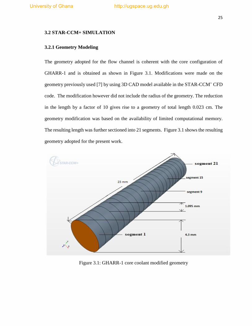
3.2.1 Geometry Modeling

The geometry adopted for the flow channel is coherent with the core configuration of

GHARR-1 and is obtained as shown in Figure 3.1. Modifications were made on the

geometry previously used [7] by using 3D CAD model available in the STAR-CCM+ CFD

code. The modification however did not include the radius of the geometry. The reduction

in the length by a factor of 10 gives rise to a geometry of total length 0.023 cm. The

geometry modification was based on the availability of limited computational memory.

The resulting length was further sectioned into 21 segments. Figure 3.1 shows the resulting

geometry adopted for the present work.

Figure 3.1: GHARR-1 core coolant modified geometry


26

3.2.2 Mesh Generation

The mesh generation pipeline consisted of surface remesher, polyhedral mesher and prism

layer mesher. The surface remesher is chosen to re-triangulate the existing surface in order

to improve the overall quality of the surface and optimize it for the volume mesh models.

The polyhedral meshing model was utilized with the prism layer mesh in order to generate

orthogonal prismatic cells next to the wall boundaries. This layer of cells is necessary to

improve the accuracy of the flow solution. The choice of the polyhedral mesh is to take

advantage of its short turnaround time in building the mesh with solution accuracy and

convergence rate. The properties of the meshing models adopted are shown in Table 3.1.

Table 3.1: Meshing Models

S/No Mesh Models Specification

1 Base Size 0.12mm

2 Prism Layer Stretching 1.11

3 Prism Layer Thickness 0.5 mm

4 Number of Mesh cells 553928

5 Surface growth rate 1.3

6 Number of Prism Layers 20

The resulting mesh generated after applying the above mesh models for the modified

geometry is presented in Figure 3.2.


27

Figure 3.2: Mesh scene

3.2.3 Setting-up Physics

Physics models and boundary conditions employed for the present work are shown in table

3.2 below.

Table 3.2: Physics Model

S/No Physics Model Specification

1 Space Model Three Dimensional

2 Time Model Steady State

3 Material Model Water

4 Flow Model Segregated Flow

5 Energy Model Segregated Fluid Isothermal

6 Viscous Regime Model Turbulent

7 Turbulent Model K-Epsilon

8 K-E Model Standard K-E Turbulence

9 Wall Function All Y+ Wall Treatment

10 Convection Scheme 2nd Order

Boundary Condition Specification

11 Inlet Mass Flow Inlet

inlet Temperature

13 Interface Free Stream

14 Outlet Pressure outlet

15 wall Surface heat Flux


28

Segregated Flow model which is a suitable flow model for liquid material model was

chosen in order to solve the required flow equations in an uncoupled manner. The linkage

between the momentum and continuity equations is achieved with a predictor-corrector

approach. This model has its roots in constant-density flows adequate for the steady state

system presently studied. It is capable of handling mildly compressible flows and low

Raleigh number natural convection. Unlike coupled flow which needs more resources like

memory and computational time as it solves coupled equations for pressure and velocities.

The segregated flow model choice for the present study was due to memory availability

limitation. The model is suitable for the studied material model whose density. The

segregated fluid isothermal model was applied as the energy model to provide constant

temperature field for all models that required temperature. In order to work with the three

dimensional mesh, a three-Dimensional model was selected. The Steady model is selected

because the system under study is a steady state system. When this model is activated, the

concept of a physical time-step is meaningless. Second order Convection scheme was

chosen for accuracy and stability of the solution. The all y+ wall treatment was selected

because it is a hybrid treatment that attempts to emulate the high y+ wall treatment for

coarse meshes and the low y+ wall treatment for fine meshes.

Thermometric input parameters (temperature, density, viscosity, and thermal conductivity)

needed as boundary conditions were computed using the NIST online database. The

computed thermometric properties are presented in Appendix A. The parameters were

imposed at both the inlet and outlet and also on the surface boundaries. Figure 3.3 shows

the boundary conditions adopted for the STAR-CCM+ simulation.


29

Figure 3.3: cylindrical flow channel showing imposed boundary conditions

For each power level mass flow rate and temperature were imposed as boundary conditions

at the inlet. On the wall surface, a varying heat flux was imposed. The varying heat flux

takes into consideration the power peaking factor for each segment. Pressure was imposed

at the outlet.

Standard k-ɛ turbulence model available in the STAR-CCM+ code was adopted for the

present study. The k-ɛ turbulence model is a two-equation model in which the equations

for turbulent kinetic energy and its dissipation are solved. The modelled equations for k

and ɛ and their coefficients are given in equations 2.6 and 2.7 respectively.

The governing equations of flow namely; continuity equation, energy equation and

momentum equations given in equations 2.1 - 2.5 are solved over the domain. The solution

were monitored to converge by assessing the residuals (Appendix F) and the trend of the

outlet temperature. Figure 3.4 depicts contour plots of the fluid temperature development.

After set-up, the simulation iterate for about 20 seconds before the onset of fluid


30

development. Hence at 0-19 s given by Figure 3.4a the temperature scene is equal to the

inlet temperature. Figure 3.4b shows the wall surface temperature distribution after 20 s.

This temperature contour is influenced by the pattern of the imposed wall surface heat flux.

Almost immediately, the temperature from the imposed heat flux is distributed marking the

onset of temperature development within the fluid. In figure 3.4c after 3800 s the

temperature can be seen building up from the inlet to the outlet. Fluid at higher temperature

can be seen moving towards the outlet as presented in Figure 3.4d after 4500 s.

Figure 3.4: channel temperature development with time

It can be seen from Figure 3.4e and 3.4f that as the simulation progresses, the temperature

distribution varies from inlet to outlet over time until it stabilizes after 5160 s when there

is no significant difference in the temperature distribution on the wall surface. Figure 3.4f

shows the temperature contour after 5400 s.


31

3.3 POWER PEAKING FACTORS CALCULATION

Computation of GHARR-1 power peaking factors was done by dividing each of the 344

fuel pins in the GHARR-1 core into 21 axial segments [7]. The temperature for each of

these segments was calculated using MCNP neutronic code. The maximum temperature

for each of the 21 axial segments was used to represent the temperature of the hottest

channel. An average of the temperature for the 344 fuel pins was taken as the temperature

of the averaged channel. The total calculated temperatures (344 × 21) were averaged to

get the core average temperature. To calculate the power peaking factor, each of the 21

temperature values for hottest and averaged pins was divided over the core average. Table

3.3 gives the resulting power peaking factors for hottest and averaged channels.

Table 3.3: Power Peaking Factors for GHARR-1 Core [7].

Axial

segment

Hottest

Channel

Averaged

channel

1 1.20363754 1.017745586

2 1.122930233 0.941616129

3 1.133713187 0.954228422

4 1.171182012 0.986920571

5 1.225387689 1.024269794

6 1.265911039 1.059170889

7 1.304844097 1.087226271

8 1.323840326 1.108510771

9 1.341304445 1.121339658

10 1.339559002 1.124731595

11 1.323064574 1.118235095

12 1.308936189 1.104893912

13 1.281755775 1.079923035

14 1.245305124 1.046968555

15 1.183962528 1.005700206

16 1.126624752 0.955673981

17 1.061025217 0.902197271

18 0.986058474 0.846280419

19 0.940349222 0.800489936

20 0.933006729 0.791342411

21 1.052918607 0.911237107


32

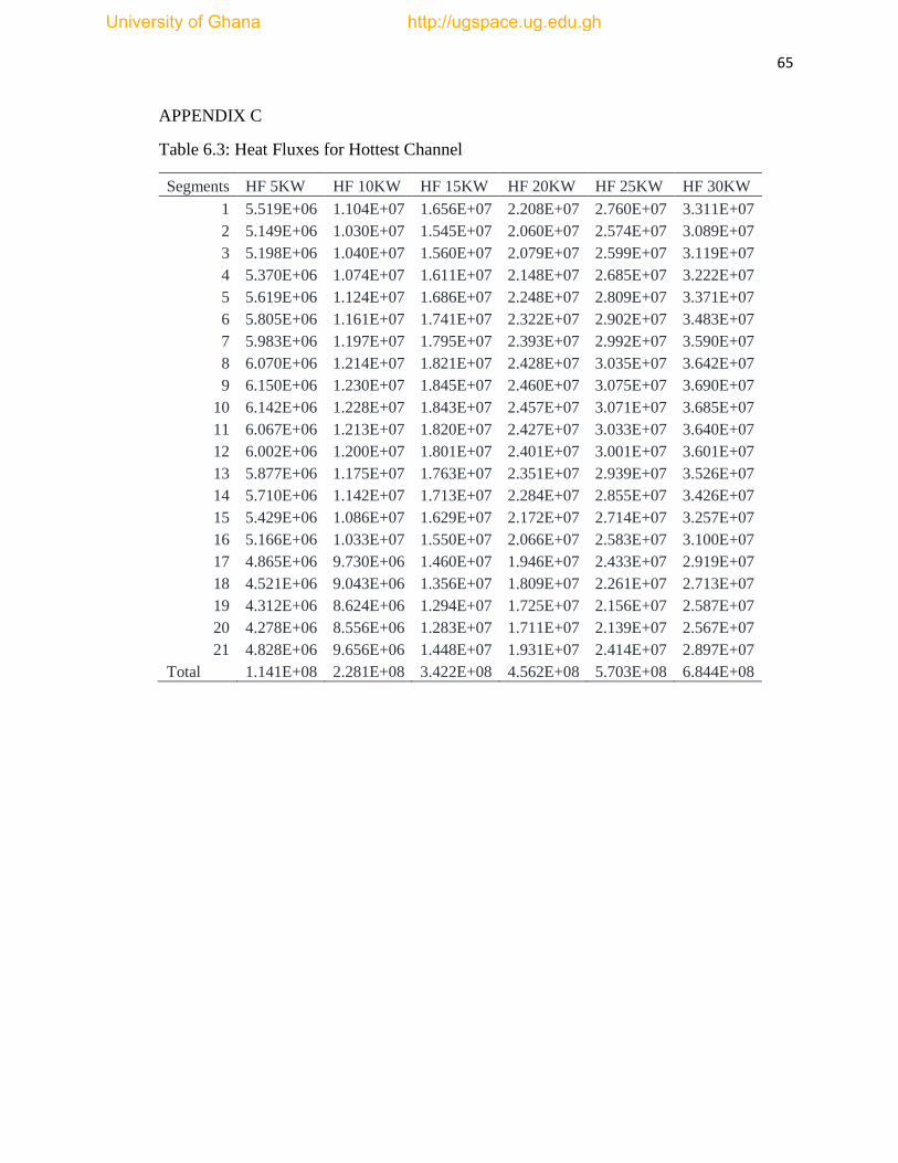
3.4 HEAT FLUX CALCULATION FOR THE MODIFIED GEOMETRY

The power peaking factors presented in Table 3.5 were used to calculate the imposed heat

flux for each segment using equation 3.2. The computed heat fluxes are presented in

Appendixes B and C.

ss

s

P

A (3.2)

Where As is the surface area of the segment given by equation 3.3, s is the segment

heat flux and sP is the segment power given by equation 3.4

𝐴 = 2𝜋rh + 2𝜋𝑟2 (3.3) Where r = segment radius, h = segment length. However, because of the geometry

modification, the height was reduced from 10.95 mm to 1.095 mm.

𝑃𝑠 = (𝑓𝑠

𝑓𝑇) ∗ 𝑃𝑅 (3.4)

Where Ps is the segment power, fs is the segment power peaking factor, fT is the total power

peaking factor and PR is the reactor power considered.

The resulting heat flux calculated for hottest and averaged channels are presented in

appendix B and appendix C respectively.

Data obtained from the simulation was post-processed and plots were generated for

analysis. The simulation generated results were validated with experimental data. In the

next chapter, discussion of trends of plots generated from simulation data is presented.


33

CHAPTER 4

RESULTS AND DISCUSSION

4.1 INTRODUCTION

In this chapter details of results obtained from both experimental and simulation exercises

are presented and discussed. Results of the simulation were obtained over constrained

planes and line probes. Figure 4.1 shows the constrained planes. The constrained planes

were placed at the inlet and outlet of each segment.

Figure 4.1: Position of constrained planes in the geometry

The solutions were also taken over line probes that are shown in figure 4.2. The line probes

were placed at different points on the surface and within the fluid. Eight line probes were

placed close to the wall and one at the center of the geometry. From the centerline probe,

the next probe was placed at a distance of 2 mm and the subsequent line probes were placed

at an increased distance of 0.02 mm interval.

Figure 4.2: Position of line probes in the geometry


34

4.2 VALIDATION OF SIMULATION DATA

In order to determine the extent of prediction of the experimental data, plots of outlet

temperature against power for the simulation were compared with data obtained

experimentally. “Out Temp Exp”, “Out Temp Sim Hot” and “Out Temp Sim Avr” used in

the legend are abbreviations for experimental outlet temperature, simulation outlet

temperature for hottest channel and simulation outlet temperature for averaged channel

respectively. In the present work, hottest channel is the channel whose segment heat fluxes

are calculated using the GHARR-1 power peaking factors for hottest channel presented in

Table 3.6. Averaged channel is the channel whose segment heat fluxes were computed

using the GHARR-1 power peaking factors for the averaged channel presented in Table

3.3.

Figures 4.3a and 4.3b shows plots of temperature against power for a uniform mass flow

rate of 0.15 kg/s.

Figure 4.3a: Graph of outlet Temperature versus Power for hottest channel

42

47

52

57

62

67

72

77

5 10 15 20 25 30

TE

MP

ER

AT

UR

E/O

C

POWER/kW

Out Temp Exp Out Temp Sim Hot


35

Figure 4.3b: Graph of outlet Temperature versus Power for averaged channel

In Figures 4.3a and 4.3b, a mass flow rate of 0.15 kg/s was used for simulation at 5 kW –

30 kW. This mass flow rate corresponds to the mass flow rate stated for normal operation

of GHARR-1 [3]. The simulated result for 5kW to 15 kW agrees closely with the

experimental result but between 15 kW and 30 kW, a marked deviation of the simulation

data from the experimental was observed. The deviation observed could be due to

inadequate cooling which led to ineffective removal of heat generated at 20 kW to 30kW.

The mass flow rate in the 30 kW power was increased in order to investigate the effect of

increased coolant volume on the simulation outlet temperature. Figures 4.4a and 4.4b show

plots of temperature against power obtained after varying the mass flow rate for the

simulation at 30 kW from 0.15 kg/s to 0.2 kg/s.

42

47

52

57

62

67

72

77

5 10 15 20 25 30

TE

MP

ER

AT

UR

E/O

C

POWER/kW

Out Temp Exp Out Temp Sim Avr


36

Figure 4.4 a: Graph of outlet Temperature versus Power for hottest channel

Figure 4.4 b: Graph of outlet Temperature versus Power for averaged channel

42

47

52

57

62

67

5 10 15 20 25 30

TE

MP

ER

AT

UR

E/O

C

POWER/kW


42

47

52

57

62

67

5 10 15 20 25 30

TE

MP

ER

AT

UR

E/O

C

POWER/kW



37

In Figures 4.4a and 4.4b, the result of increasing the mass flow rate for 30 kW for the same

condition led to a reduction on the deviation observed for 30 kW data point in Figure 4.3a

and 4.3b.

The observed effect of varying mass flow rate for the simulation at 30 kW informed the

need to also increase the mass flow rates for the simulation at 20 kW to 30 kW. Figures

4.5a and 4.5 b shows plots of temperature against power obtained after varying the mass

flow rate for the simulation at 20 kW and 25 kW from 0.15 kg/s to 0.18 kg/s and 0.20

kg/s respectively. The simulation at 30 kW was also further increased from 0.20 kg/s to

0.23 kg/s.

Figure 4.5 a: Graph of outlet Temperature versus Power for hottest channel

42

47

52

57

62

5 10 15 20 25 30

TE

MP

ER

AT

UR

E/O

C

POWER/kW



38

Figure 4.5 b: Graph of outlet Temperature versus Power for averaged channel

The result in Figure 4.5a and 4.5b show a significant reduction in the deviation of the data

points for 20 kW to 30 kW and therefore, the data obtained from the simulation show a

better agreement with the experimental. It is found that increasing mass flow rate enhances

the heat transfer rate leading to a decrease in the outlet temperature. The effect of mass

flow rate on outlet temperature is presented in Table 4.1.

Table 4.1: Mass flow rate on outlet temperature at 30 kW

mass flow rate Texp Thot Tavr Thot - Texp Tavr - Texp Thot - Tavr

0.15 58.11 73.17 73.57 15.06 15.46 0.4

0.20 58.11 62.63 62.80 4.52 4.69 0.17

0.23 58.11 59.14 59.24 1.03 1.13 0.10

When the mass flow rate for 30 kW was increased from 0.15 kg/s to 0.23 kg/s, the

difference between the experimental outlet temperature and the simulation outlet

temperature decreased for both averaged and hottest channels as presented is Table 4.1.

42

44

46

48

50

52

54

56

58

60

5 10 15 20 25 30

TE

MP

ER

AT

UR

E/O

C

POWER/kW



39

For 34.8% increase in the mass flow rate, the percentage decrease in temperature between

the hottest channel and the experimental data was found to be 93.2% while that between

the averaged channel and the experimental data was 92.7%. The decrease in temperature

between the hottest channel and averaged channel was also found to be 75%. The

percentages were calculated using equations 4.1 and 4.2.

(𝑇ℎ𝑜𝑡 − 𝑇𝑒𝑥𝑡)0.15 − (𝑇ℎ𝑜𝑡 − 𝑇𝑒𝑥𝑡)0.23

(𝑇ℎ𝑜𝑡 − 𝑇𝑒𝑥𝑡)0.15 (4.1)

(𝑇𝑎𝑣𝑟 − 𝑇𝑒𝑥𝑡)0.15 − (𝑇𝑎𝑣𝑟 − 𝑇𝑒𝑥𝑡)0.23

(𝑇𝑎𝑣𝑟 − 𝑇𝑒𝑥𝑡)0.15 (4.2)

where,

𝑇𝑒𝑥𝑡 = experimental outlet temperature

𝑇𝑎𝑣𝑟 = Simulation outlet temperature for the averaged channel

𝑇ℎ𝑜𝑡 = Simulation outlet temperature for the hottest channel

It is observed that a very close agreement with the experimental data will be obtained by

further increasing the mass flow rate for the simulation at 20 kW to 30 kW. Generally, the

trend of the simulation plots show that as power increases, there is a build-up of heat within

the core. Hence there is need to allow more coolant into the system for efficient heat

removal. STAR-CCM+ CFD code is able to predict heat transfer and distribution in the

core of GHARR-1 at the power levels considered.


40

4.3 DISTRIBUTION OF WALL Y+ IN THE DOMAIN

The wall y+ was taken as an average over each segment and plotted against power. The

evaluated result is presented in Figure 4.6. The all y+ wall treatment was chosen for the

adopted k-e model. The all y+ wall treatment was employed due to its versatility to give

reasonable results on coarse meshes for y+ > 30 and on fine meshes for y+ ≤ 1 [27].

Figure 4.6: Wall y+ distribution over the domain.

For all power levels the wall y+ value decreases progressively along the flow channel and

has its lowest value at the outlet. From the graph wall y+ increases with increasing power

this is due to its dependence on density, velocity and kinematic viscosity as presented in

equation 4.3. The dimensionless wall y+ is related to the wall distance y from the prism

layer cell by equation 4.3

5

6

7

8

9

10

11

12

1 3 5 7 9 11 13 15 17 19 21

WA

LL Y

+

SEGMENT

5 kW_hot 10 kW_hot 15 kW_hot 20kW_hot 25kW_hot 30kW_hot


41

𝑦+=𝑦

𝑣√

𝜏𝑤

𝜌 (4.3)[27]

Where, 𝜏𝑤 is the wall shear stress, 𝜌 is the density and v is the kinematic viscosity.

4.4 SURFACE AVERAGE TEMPERATURE

Surface average temperatures was obtained as an average over each segment. “SAT

5kW_Hot and SAT 5kW_Avr” used in the legend are abbreviations for surface average

temperature taken over each segment for the simulation at 5 kW for the hottest channel and

averaged channel respectively. Figure 4.7 a. and 4.7 b. show the variation of the surface

temperature with position for hottest channel and averaged channel respectively.

Figure 4.7 a: Surface Average Temperature versus Position for hottest channel

70

120

170

220

270

320

370

420

470

1 2 3 4 5 6 7 8 9 10 11 12 13 14 15 16 17 18 19 20 21

SUR

FAC

E A

VER

AG

E TE

MP

ERA

TUR

E /O

C

SEGMENT

SAT 5kW_Hot SAT 10kW_Hot SAT 15kW_Hot

SAT 20kW_Hot SAT 25kW_Hot SAT 30kW_Hot


42

Figure 4.7 b: Surface Average Temperature versus Position for averaged channel

The result shows that the surface average temperature increases with increase in power.

For both hottest and averaged channels, the surface average temperatures are lowest at the

inlet and peaks at a value at the 12th segment. For all powers, the peak experienced a steady

decrease from segment 14 to 19 before rising at segment 20. The lowest surface

temperature is recorded for the simulation 5 kW in both hottest and averaged channels.

Table 4.2 presents an evaluation on the trend difference for power level consideration.

Table 4.2: surface temperature for varying power levels.

Power (kW)

Segment 1 surface

temperature

Change in

temperature

30 222.8

25 215.1 7.7

20 183.7 31.4

15 161.3 22.4

10 124.4 36.9

5 84.1 40.3

70

120

170

220

270

320

370

420

470

1 2 3 4 5 6 7 8 9 10 11 12 13 14 15 16 17 18 19 20 21

SUR

FAC

E A

VER

AG

E TE

MP

ERA

TUR

/OC

AXIS TITLE

SAT 5kW_Avr SAT 10kW_Avr SAT 15kW_Avr

SAT 20kW_Avr SAT25 kW_Avr SAT 30kW_Avr


43

From the table 4.3, the least difference in the trends exist between trends for simulation at

30 kW and 25 kW. This result is in agreement with the result of local distribution of surface

temperatures previously recorded [1] where the local surface temperature increases with

the increase in the heat flux. In addition, with the local surface temperature increasing

towards the outlet of the channel.

4.5 BULK AVERAGE TEMPERATURE

The fluid bulk average temperature was taken over each segment with the aid of constraint

planes placed at the inlet and outlet. This is done to determine the temperature distribution

within the fluid. Figure 4.8 a. and 4.8 b. shows variation of bulk average temperature with

position taken over each segment for hottest and averaged channels respectively. “BAT

5kW_Hot and BAT 5kW_Avr” used in the legend are abbreviations for fluid bulk average

temperature taken over each segment for the simulation at 5 kW for the hottest channel and

averaged channel respectively.

Figure 4.8 a: Bulk Average Temperature versus Position for hottest channel

37

42

47

52

57

62

1 2 3 4 5 6 7 8 9 10 11 12 13 14 15 16 17 18 19 20 21

BU

LK

AV

ER

AG

E T

EM

PE

RA

TU

RE

/OC

SEGMENT

BAT 5kW_Hot BAT 10kW_Hot BAT 15kW_Hot

BAT 20kW_Hot BAT 25kW_Hot BAT 30kW_Hot


44

Figure 4.8 b: Bulk Average Temperature versus Position for averaged channel

The general trend shows an increase in the fluid temperature along the channel. It also

shows greater variation in the temperature along the channel with a maximum variation at

the exit. This suggest that as the fluid moves upwards in the channel more heat is extracted

from the fuel. The trend is consistent for 5, 10, 15 and 20 kW powers but different for 25

and 30 kW due to increase in mass flow rate.

The trend for bulk average temperature conforms to that previously reported [1] where the

local coolant temperature increases with the increase in the coolant inlet temperature. In

addition, increase in the local coolant temperature along channel is higher close to the outlet

of the channel.

37

42

47

52

57

62

1 2 3 4 5 6 7 8 9 10 11 12 13 14 15 16 17 18 19 20 21

BU

LK

AV

ER

AG

E T

EM

PE

RA

TU

RE

/OC

SEGMENT

BAT 5kW_Avr BAT 10kW_Avr BAT 15kW_Avr

BAT 20kW_Avr BAT 25kW_Avr BAT 30kW_Avr


45

4.6 SURFACE AND BULK TEMPERATURE COMPARISON

The surface average and fluid bulk average temperatures are compared in order to study

the extent to which heat is extracted from the surface to the bulk of the fluid. Figures 4.9

shows a plot for surface average temperature and fluid bulk average temperature taken for

the simulation at 15 kW for hottest channel.

Figure 4.9: Surface and Bulk Temperature for hottest channel versus Position for 15kW

The result shows an increase in both the surface and fluid bulk average temperature from

inlet to outlet. However, the trend for surface average temperature shows a sharp rise

between segment 1 and 8 followed by a slight rise between segment 8 and 11. Between

segment 11 and 19 the trend is a downwards curve followed by another rise between

segment 20 and 21. The temperature on the surface is due to the applied heat on the wall

surface. The resulting fluid bulk temperature suggests that the heat is conducted in such a

way that the fluid bulk temperature remain in liquid phase two phase flow is attained. The

resulting outlet temperature is within a range that can be cooled by natural convection. No

38

88

138

188

238

288

338

1 3 5 7 9 11 13 15 17 19 21

TE

MP

ER

AT

UR

E/O

C

SEGMENT

SAT 15kW_Hot BAT 15kW_Hot


46

correlation was observed between the surface average and the fluid bulk average

temperature trends.

However addition of 7 line probes between the surface and the fluid centerline gives a

correlated temperature distribution presented in Figure 4.10. The number in the parenthesis

in the legend gives the distance of the probe point from the fluid centerline.

Figure 4.10: Temperature distribution trend close to boundary layer

The result shows the temperature increasing along the channel from inlet to outlet. The

trend shows the curve flattening from the surface to the fluid centerline. Temperature

distribution at the boundary layer is greatest at the wall where the heat flux is applied.

4.7 BULK AVERAGE TURBULENT INTENSITY

The fluid bulk turbulent intensity was calculated as an average over each segment to

investigate the degree of turbulence in the various segments of the GHARR-1 core. The

30

80

130

180

230

280

-0.002 0.003 0.008 0.013 0.018 0.023

TEM

PER

ATU

RE/

OC

POSITION/m

probe 2 (0.00214) probe 1 (0.00) probe 3 (0.00212)




47

turbulent intensity was computed using equations 4.3 and 4.4 and the results evaluated are

plotted in Figures 4.11a and 4.11b.

𝐼 =ύ

ṽ (4.3)

where ṽ is the mean flow velocity (computed using Appendix D) and

ύ = √2

3𝑘 (4.4)

where k is the turbulence kinetic energy (Appendix C).

Figures 4.11a and 4.11b show a graph of turbulent intensity versus position for hottest and

averaged flow channels respectively. “TI 5kW_hot and TI 5kW_avr” used in the legend

are abbreviations for turbulent intensity taken over each segment for the simulation at 5

kW for the hottest channel and averaged channel respectively.

Figure 4.11a: Bulk Average Turbulent Intensity versus Position for hottest channel

0.0165

0.0185

0.0205

0.0225

0.0245

0.0265

0.0285

0.0305

1 2 3 4 5 6 7 8 9 10 11 12 13 14 15 16 17 18 19 20 21

TUR

BU

LEN

T IN

TEN

SITY

SEGMENT

TI 5kW_hot TI 10kW_hot TI 15kW_hotTI 20kW_hot TI 25kW_hot TI 30kW_hot


48

Figure 4.11b: Turbulent Intensity versus Position for averaged channel.

The turbulence values recorded at the inlet segment increased sharply between segments 1

and 2 for simulations at 15 kW to 30 kW. Between segments 3 and 7, turbulence intensity

values decreased for the simulations at 15 kW to 30 kW. The sharp increase and subsequent

decrease in turbulent intensity observed between segments 1 and 7 could be attributed to

the initiation of flow development in the channel. From the 7th segment, steady rise in

turbulence intensity was observed through to the exit of the domain. The development of

the flow from the 7th segment could be said to be more appreciable than that observed

between segments 1 and 7.

The turbulent intensity observed at lower powers of 5 kW and 10 kW were higher in

magnitude than those observed at 15 kW to 30 kW. This is as a consequence of the inverse

proportionality relationship existing between turbulent intensity and velocity. Hence the

0.0165

0.0185

0.0205

0.0225

0.0245

0.0265

0.0285

0.0305

1 2 3 4 5 6 7 8 9 10 11 12 13 14 15 16 17 18 19 20 21

TUR

BU

LEN

T IN

TEN

SITY

SEGMENT

TI 5kW_avr TI 10kW_avr TI 15kW_avr

TI 20kW_avr TI 25kW_avr TI 30kW_avr


49

higher coolant velocities obtained at higher powers of 15 kW to 30 kW contributed to the

lower turbulent intensities and vice versa.

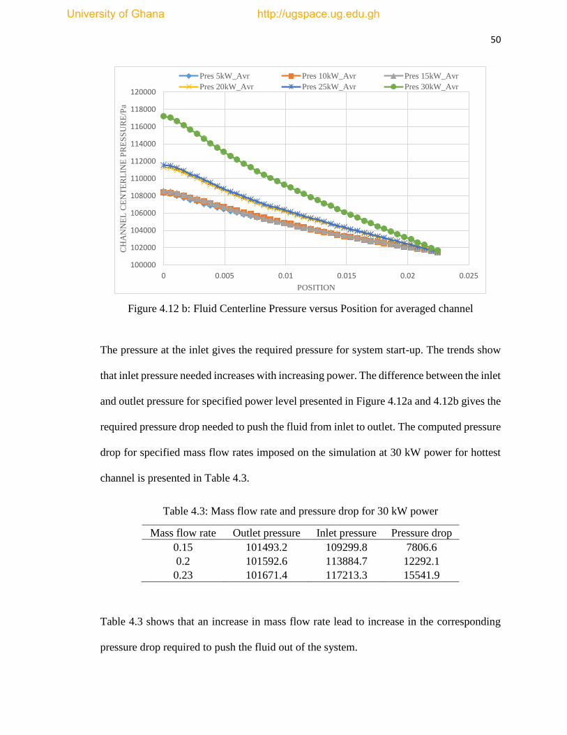
4.8 CHANNEL CENTERLINE PRESSURE

The channel centerline pressure was taken using a line probe placed at the center of the

geometry to analyze trend of the pressure across the domain. Figures 4.12a and 4.12b show

the plot of fluid centerline pressure versus position for simulation at 5 kW to 30 kW for

average and hottest channel respectively. “Pres 5kW_Hot and Pres 5kW_Avr” used in the

legend are abbreviations for channel centerline pressure taken over each segment for the

simulation at 5 kW for the hottest channel and averaged channel respectively.

Figure 4.12 a: Fluid Centerline Pressure versus Position for hottest channel

101000

103000

105000

107000

109000

111000

113000

115000

117000

119000

0 0.005 0.01 0.015 0.02 0.025

CH

AN

NE

L C

EN

TE

RL

INE

PR

ES

SU

RE

/Pa

POSITION

Pres 5kW_Hot Pres 10kW_Hot Pres 15kW_Hot

Pres 20kW_Hot Pres 25kW_Hot Pres 30kW_Hot


50

Figure 4.12 b: Fluid Centerline Pressure versus Position for averaged channel

The pressure at the inlet gives the required pressure for system start-up. The trends show

that inlet pressure needed increases with increasing power. The difference between the inlet

and outlet pressure for specified power level presented in Figure 4.12a and 4.12b gives the

required pressure drop needed to push the fluid from inlet to outlet. The computed pressure

drop for specified mass flow rates imposed on the simulation at 30 kW power for hottest

channel is presented in Table 4.3.

Table 4.3: Mass flow rate and pressure drop for 30 kW power

Mass flow rate Outlet pressure Inlet pressure Pressure drop

0.15 101493.2 109299.8 7806.6

0.2 101592.6 113884.7 12292.1

0.23 101671.4 117213.3 15541.9

Table 4.3 shows that an increase in mass flow rate lead to increase in the corresponding

pressure drop required to push the fluid out of the system.

100000

102000

104000

106000

108000

110000

112000

114000

116000

118000

120000

0 0.005 0.01 0.015 0.02 0.025

CH

AN

NE

L C

EN

TE

RL

INE

PR

ES

SU

RE

/Pa

POSITION

Pres 5kW_Avr Pres 10kW_Avr Pres 15kW_Avr

Pres 20kW_Avr Pres 25kW_Avr Pres 30kW_Avr


51

4.9 CONTOUR PLOTS FOR HOTTEST CHANNEL SIMULATION AT 30 kW

Contour plots are presented over constrained planes in other to visualise the heat transfer

and distribution from the surface to the bulk fluid at different positions in the domain. The

plots taken at inlet, outlet and middle segments are presented in Figures 4.13 to 4.15.

Figure 4.13: Inlet segment temperature distribution

Figure 4.14: Temperature distribution in the middle segment


52

Figure 4.15: outlet segment temperature distribution

Figure 4.13 shows a uniform distribution of temperature over the interface. The interface

temperature was observed to be the same as the inlet temperature. Figure 4.14: shows an

decrease in temperature from the surface to the bulk of the fluid. It also shows the

effectiveness of the coolant to remove heat from the fuel rod surface. This can be seen in

the manner at which high surface temperature is removed without heating the bulk of the

fluid. Compared to Figure 4.13, there is a build of temperature at the region around the wall

boundary in Figure 4.14. Figure 4.15 shows a boundary temperature development of

greater magnitute than those observed in Figures 4.13 and 4.14. This implies that the

temperature close to the walls increases along the domain.

The contour plot of domain surface temperature shows temperature distribution on the

surface of the flow channel. Figure 4.16 gives the contour plot for domain surcae

temperature.


53

Figure 4.16: Surface temperature distribution

The contour shows the surface temperature is least between segment 1 and 9 peaking at the

middle of between segment 10 and 15 before dropping to a lesser temperature between

segment 16 and 21. The surface temperature distribution follows the same trend as the

power peaking factors presented in Table 3.3.

4.10 COEFFICIENT OF HEAT TRANSFER

The coefficient of heat transfer was calculated for each segment using equations 4.5 and

4.6. The result of the evaluated heat transfer coefficient is plotted against the segment as

presented in Figure 4.17.

ℎ =𝑞

𝐴𝑠∆𝑇 (4.5).

∆𝑇 = 𝑇𝑠 − 𝑇𝑏 (4.6)

where As is the surface area, q is segmental power, Ts is surface temperature, Tb is the bulk

temperature


54

Figure 4.17 gives a plot of coefficient of heat transfer against segment for simulations at

30 kW. “CHT_30kW hot and CHT_30kW avr” used in the legend are abbreviations for

coefficient of heat transfer for hottest and averaged channels respectively.

Figure 4.17: Coefficient of heat transfer versus Position

The trend shows the highest heat transfer coefficient exist at segment 1 followed by a

progressive reduction up to segment 20 before a slight rise between segment 20 and 21.

Findings of the analysis performed for heat transfer and distribution in GHARR-1 core has

been presented. Conclusion on the above discussed results will be drawn in the next

Chapter.

300000

350000

400000

450000

500000

550000

600000

650000

700000

750000

1 2 3 4 5 6 7 8 9 10 11 12 13 14 15 16 17 18 19 20 21

CO

EFFI

CIE

NT

OF

HEA

T TR

AN

SFER

SEGMENT

CHT_30kW hot CHT_30kW avr


55

CHAPTER FIVE

CONCLUSION AND RECOMMENDATION

5.1 CONCLUSION

A study of heat transfer and distribution was conducted to evaluate the steady state thermal

hydraulic behavior of GHARR-1 core under natural convection cooling. Based on the

results obtained, significant conclusion are hereby drawn:

1) The surface average temperature increases along the flow channel from inlet to

outlet but peaks at the middle segments in conformity with the trends of GHARR-

1 power peaking factors presented in Table 3.3.

2) The fluid bulk average temperature increases along the flow channel. A sharp

increase in fluid bulk temperature was observed between segment 1 and 12.

However between segment 12 and 21 the rate of increase in temperature dropped

slightly. This suggests that, as the fluid develops, more heat is taken from the fuel

and transported towards the outlet. It was also observed that the fluid bulk

temperature increases with increase in power.

However lateral distribution of temperature from the surface to the fluid centerline

shows an effective heat transfer through the fluid.

3) There is a general increase in the turbulent intensity over the domain from inlet to

outlet which also increases with increase in power. This suggest that as the flow

develops, there is a build-up of turbulence in the domain. The observed trends

suggests a turbulence surge at the inlet accompanied by a turbulence drop while the

fluid stabilizes before an even greater rise in turbulent intensity. This observation


56

conforms to GHARR-1 Safety Analysis that the closer the coolant gets to the upper

part of the fuel elements, the stronger the turbulence becomes [8].

4) The fluid centerline pressure was found to increase with increase in power, this

suggest that both the required pressure for starting the system and the required

pressure drop for transporting the fluid across the domain increases with power

increase.

5) The values of outlet temperature for experimental measurements are lower than

those calculated by STAR-CCM+ CFD code by a deviation of 1% - 1.6%. With this

variation, taking into consideration meshing model dynamics, it is concluded that

STAR CCM+ has predicted the studied physical parameters.

6) The present study has predicted the trend of the measured parameters as fluid

develops from inlet to outlet of modified GHARR-1 core. This provides more

insight about the distribution of mean and turbulent flow parameters for GHARR-

1 core.

7) The failure to predict power beyond 31.2 kW in PLTEMP/ANL transient analysis

in [7] informed the need to restrict the present steady state studies to 30 kW power

level. The results from the present steady state reaffirms those obtained from the

PARET/ANL transient simulations which indicates that Ghana Research Reactor-

1 is safe to operate at the at a nominal power of 30 kW.

5.2 RECOMMENDATIONS

The present work should be extended to include thermal hydraulics study of GHARR-1

core subchannel to enable a more general conclusion on heat transfer and distribution. Also


57

other CFD codes should be studied using the same conditions as the present study for

verification. A full geometry of GHARR-1 core should be modelled and simulated using

STAR-CCM+ for heat transfer analysis with the view of updating GHARR-1 Safety

Analysis Report book. The present work should be extended to study GHARR-1 core heat

transfer and distribution during accident and transient conditions.


58

REFERENCES

[1] Talha K. A., Acbdel-Hadi E. A., El-Ghnam R. I., Taher S. H. and Abdel-Latif S.

H. (2012). Thermal Hydraulic Behavior of Research Reactor during Natural

Convection Cooling Mode. Arab Journal of Nuclear Science and Applications, 45:4

243-256.

[2] Annafi T. A., Gyeabour A. A., Akaho E. H. K., Annor-Nyarko M. and Quaye C. R.

(2014). Finite Difference Analysis of the Transient Temperature Profile within Gharr-

1 Fuel Element. International Journal of Scientific and Technology Research. 3:8 2277-

8616.

[3] Akaho E.H.K., Maaku B.T., Anim Sampong S., Emi-Reynolds G, Boadu H.O, ,

Dodoo-Amoo D.N.A. (2006). Ghana Research Reactor-1, Final Safety Analysis

Report. GAEC, Kwabenya, Ghana.

[4] Sogbadji R. B.M. (2012). Neutronic Study of the Mono-Recycling Of Americium

in PWR and Of the Core Conversion in MNSR Using the Mure Code. Research Thesis

submitted to Universite De Paris Sud.

[5] Odoi H., Akaho E. H. K., Anim-Sampong S., Jonah, Nyarko, S. B. Abrefah R.,

Ampomah-Amoako E., Sogbadji R B. M., Lawson I., Birinkoranga S., Ibrahimc Y. and

Boffie J. (2011). Investigative studies on effect of reflector thickness on the

performance of low enriched uranium-fuelled MNSR’s. Nuclear Engineering and

Design 241:8 2902-2915.

[6] Sogbadji R B M., Abrefah R., Ampomah-Amoako, E Agbemava. S. and Nyarko B.

J.B. (2011). Neutron energy spectrum flux profile of Ghana’s miniature neutron source

reactor core. Annals of Nuclear. Energy 38:8 1787-1792.

[7] Ampomah-Amoako E., Akaho E.H.K., Anim-Sampong S., Nyarko B.J.B. (2009).

Transient Analysis of Ghana Research Reactor-1 using PARET/ANL thermal–

hydraulic code. Nuclear Engineering and Design 239: 2479–2483.


59

[8] Akaho E.H.K., Maakuu B.T., Anim-Sampong S., Emi-Reynolds G., Boadu H.O.,

Osae E.K., Akoto S. B., Dodoo-Amoo D.N.A. (2003). Ghana Research Reactor-1

Safety Analysis Report. GAEC-NNRI-RT-90

[9] Lienhard IV J. H, Lienhard V J. H. (2008). A Heat Transfer Textbook, third edition.

Phlogiston Press, Cambridge, Massachusetts, USA p 137

[10] https://en.wikipedia.org/wiki/Natural_convection 17/04/20015

[11] http://encyclopedia2.thefreedictionary.com/single-phase+flow 24/03/2015

[12] Akaho E. H. and Maaku B. T. (2002). Simulation of transients in a miniature

neutron source reactor core. Nuclear Engineering and Design. 213:1 31-42

[13] Appiah R. (2011). Steady State Thermal-Hydraulics Analysis of GHARR-1 using

the PL TEMP/ANL v4.0 Code. University of Ghana, Accra, Ghana.

[14] Costa A. L., Reis P. A. L., Silva C. A. M., Pereira C., Veloso M. A. F., Guerra B.

T., Soares H. V. and Mesquita A. Z. (2011). Safety Studies and General Simulations of

Research Reactors Using Nuclear Codes, Nuclear Power - System Simulations and

Operation, Dr. Pavel Tsvetkov (Ed.),

[15] Böck H. and Villa M. (2001). Survey of Research Reactors, prepared for the IAEA

Course on "Safety, Management and Utilization of Research Reactors". Bratislava-

Vienna.

[16] Sunniva S. T. (2013). Simulation of Viscous Flow around a Circular Cylinder

with STAR-CCM+. A Master’s Degree Thesis submitted to the Norwegian University

of Science and Technology, Department of Marine Technology

[17] Ganesh V. (2012). Understanding CFD Simulation Process with Examples

https://ganeshvisavale.wordpress.com/2012/12/07/understanding-cfd-simulation-

process-with-examples/

[18] STAR-CCM+ User Guide version 6.04.014 CD_ADAPCO 2011.


https://en.wikipedia.org/wiki/Natural_convection

http://encyclopedia2.thefreedictionary.com/single-phase+flow

https://ganeshvisavale.wordpress.com/author/ganeshvisavale/

https://ganeshvisavale.wordpress.com/2012/12/07/understanding-cfd-simulation-process-with-examples/

https://ganeshvisavale.wordpress.com/2012/12/07/understanding-cfd-simulation-process-with-examples/

60

[19] Versteeg H. K., Malalasekera, W. (2007). An Introduction to Computational Fluid

Dynamics, the Finite Volume Method. Second edition, pp. 54-128.

[20] Ampomah-Amoako E. (2013). Stability and control of Supercritical Water

Reactor System; A Study into Concepts and Applications. A Nuclear Engineering

Ph.D. Dissertation Submitted to the University of Ghana

[21] Spalart P. R., and Rumsey C.L. (2007). Effective Inflow Conditions for

Turbulence Models in Aerodynamic Calculations, AIAA Journal, 45:10 2544-2553

[22] Henkes R.A.W.M., Vander-Flugt F. F., Hoohendoorn C. J. (1991). Natural

convection in a square cavity calculated with low-Reynolds number turbulence models.

Int. J. Heat Mass Transfer, 34: 1543-1557

[23] Okon C. E., Chad-Umoren Y. E. and Abbey T. M. (2013). Thermal Profile of

Cylindrical Nuclear Reactor Fuel Elements “An Analytical Approach” Canadian

Journal on Computing in Mathematics, Natural Sciences, Engineering and Medicine

4:1

[24] Kyei A.Y., Annafi T. A., Annor-Nyarko M, Quaye C. R, Bansah C. (2014).

Modelling the Velocity Profile of Coolant Flow in the GHARR-1 Fuel Channel. Journal

of Nuclear Energy Science and Power Generation Technology

http://dx.doi.org/10.4172/2325-9809.1000123

[25] Ampomah-Amoako E., Akaho E. H.K. , Nyarko B. J.B. , Ambrosini W. (2013).

Analysis of flow stability in nuclear reactor subchannels with water at supercritical

pressures. Annals of Nuclear Energy 60: 396–405

[26] The NIST Reference on Constants, Units, and Uncertainty

http://physics.nist.gov/cuu/Units/units.html

[27] Agbodemegbe V.Y., Cheng X, Akaho E.H.K, Allotey F.K.A. (2015). Correlation

for Cross-Flow Resistance Coefficient Using STAR-CCM+ Simulation Data for Flow

of Water through Rod Bundle Supported by Spacer Grid with Split-Type Mixing Vane.

Nuclear Engineering and Design 285: 134–149.


http://dx.doi.org/10.4172/2325-9809.1000123

http://physics.nist.gov/cuu/Units/units.html

61

APPENDIX

APPENDIX A

Table 6.1: Thermophysical Properties

Temperature

(oC)

Density

(kg/m3)

Viscosity

(Pa*s)

Therm. Cond.

(W/m*K)

mass fl. rate

(kg/s)

1 9.999E+02 1.731E-03 5.630E-01 1.110E-01

2 9.999E+02 1.673E-03 5.649E-01 1.110E-01

3 1.000E+03 1.619E-03 5.668E-01 1.110E-01

4 1.000E+03 1.567E-03 5.687E-01 1.110E-01

5 1.000E+03 1.518E-03 5.706E-01 1.110E-01

6 9.999E+02 1.471E-03 5.725E-01 1.110E-01

7 9.999E+02 1.427E-03 5.744E-01 1.110E-01

8 9.999E+02 1.385E-03 5.763E-01 1.110E-01

9 9.998E+02 1.344E-03 5.782E-01 1.110E-01

10 9.997E+02 1.306E-03 5.801E-01 1.110E-01

11 9.996E+02 1.269E-03 5.819E-01 1.110E-01

12 9.995E+02 1.234E-03 5.838E-01 1.109E-01

13 9.994E+02 1.200E-03 5.857E-01 1.109E-01

14 9.993E+02 1.168E-03 5.875E-01 1.109E-01

15 9.991E+02 1.138E-03 5.894E-01 1.109E-01

16 9.990E+02 1.108E-03 5.912E-01 1.109E-01

17 9.988E+02 1.080E-03 5.931E-01 1.109E-01

18 9.986E+02 1.053E-03 5.949E-01 1.108E-01

19 9.984E+02 1.027E-03 5.967E-01 1.108E-01

20 9.982E+02 1.002E-03 5.985E-01 1.108E-01

21 9.980E+02 9.776E-04 6.002E-01 1.108E-01

22 9.978E+02 9.544E-04 6.020E-01 1.108E-01

23 9.975E+02 9.322E-04 6.038E-01 1.107E-01

24 9.973E+02 9.107E-04 6.055E-01 1.107E-01

25 9.971E+02 8.901E-04 6.072E-01 1.107E-01

26 9.968E+02 8.702E-04 6.089E-01 1.106E-01

27 9.965E+02 8.510E-04 6.106E-01 1.106E-01

28 9.962E+02 8.325E-04 6.122E-01 1.106E-01

29 9.960E+02 8.146E-04 6.139E-01 1.106E-01

30 9.957E+02 7.974E-04 6.155E-01 1.105E-01

31 9.953E+02 7.807E-04 6.171E-01 1.105E-01

32 9.950E+02 7.646E-04 6.187E-01 1.104E-01

33 9.947E+02 7.490E-04 6.203E-01 1.104E-01

34 9.944E+02 7.339E-04 6.218E-01 1.104E-01

35 9.940E+02 7.193E-04 6.233E-01 1.103E-01

36 9.937E+02 7.052E-04 6.248E-01 1.103E-01


62

37 9.933E+02 6.915E-04 6.263E-01 1.103E-01

38 9.930E+02 6.783E-04 6.278E-01 1.102E-01

39 9.926E+02 6.654E-04 6.292E-01 1.102E-01

40 9.922E+02 6.530E-04 6.306E-01 1.101E-01

41 9.918E+02 6.409E-04 6.320E-01 1.101E-01

42 9.914E+02 6.292E-04 6.334E-01 1.100E-01

43 9.910E+02 6.178E-04 6.348E-01 1.100E-01

44 9.906E+02 6.068E-04 6.361E-01 1.100E-01

45 9.902E+02 5.961E-04 6.374E-01 1.099E-01

46 9.898E+02 5.857E-04 6.387E-01 1.099E-01

47 9.894E+02 5.755E-04 6.399E-01 1.098E-01

48 9.889E+02 5.657E-04 6.412E-01 1.098E-01

49 9.885E+02 5.562E-04 6.424E-01 1.097E-01

50 9.880E+02 5.469E-04 6.436E-01 1.097E-01

51 9.876E+02 5.378E-04 6.448E-01 1.096E-01

52 9.871E+02 5.290E-04 6.459E-01 1.096E-01

53 9.867E+02 5.204E-04 6.471E-01 1.095E-01

54 9.862E+02 5.121E-04 6.482E-01 1.095E-01

55 9.857E+02 5.040E-04 6.493E-01 1.094E-01

56 9.852E+02 4.961E-04 6.503E-01 1.094E-01

57 9.847E+02 4.884E-04 6.514E-01 1.093E-01

58 9.842E+02 4.809E-04 6.524E-01 1.092E-01

59 9.837E+02 4.735E-04 6.534E-01 1.092E-01

60 9.832E+02 4.664E-04 6.544E-01 1.091E-01

61 9.827E+02 4.594E-04 6.554E-01 1.091E-01

62 9.822E+02 4.527E-04 6.563E-01 1.090E-01

63 9.816E+02 4.460E-04 6.572E-01 1.090E-01

64 9.811E+02 4.396E-04 6.581E-01 1.089E-01

65 9.806E+02 4.333E-04 6.590E-01 1.088E-01

66 9.800E+02 4.271E-04 6.599E-01 1.088E-01

67 9.795E+02 4.211E-04 6.607E-01 1.087E-01

68 9.789E+02 4.152E-04 6.615E-01 1.087E-01

69 9.783E+02 4.095E-04 6.623E-01 1.086E-01

70 9.778E+02 4.039E-04 6.631E-01 1.085E-01

71 9.772E+02 3.984E-04 6.639E-01 1.085E-01

72 9.766E+02 3.931E-04 6.647E-01 1.084E-01

73 9.760E+02 3.879E-04 6.654E-01 1.083E-01

74 9.754E+02 3.827E-04 6.661E-01 1.083E-01

75 9.748E+02 3.777E-04 6.668E-01 1.082E-01

76 9.742E+02 3.729E-04 6.675E-01 1.081E-01

77 9.736E+02 3.681E-04 6.681E-01 1.081E-01

78 9.730E+02 3.634E-04 6.688E-01 1.080E-01

79 9.724E+02 3.588E-04 6.694E-01 1.079E-01


63

80 9.718E+02 3.544E-04 6.700E-01 1.079E-01

81 9.712E+02 3.500E-04 6.706E-01 1.078E-01

82 9.705E+02 3.457E-04 6.712E-01 1.077E-01

83 9.699E+02 3.415E-04 6.718E-01 1.077E-01

84 9.693E+02 3.374E-04 6.723E-01 1.076E-01

85 9.686E+02 3.333E-04 6.728E-01 1.075E-01

86 9.680E+02 3.294E-04 6.734E-01 1.074E-01

87 9.673E+02 3.255E-04 6.739E-01 1.074E-01

88 9.666E+02 3.218E-04 6.743E-01 1.073E-01

89 9.660E+02 3.180E-04 6.748E-01 1.072E-01

90 9.653E+02 3.144E-04 6.753E-01 1.071E-01


64

APPENDIX B:

TABLE 6.2: Heat Fluxes for Averaged Channel

Segments HF 5KW

HF

10KW

HF

15KW

HF

20KW

HF

25KW

HF

30KW

1 5.54E+06 1.11E+07 1.66E+07 2.21E+07 2.77E+07 3.32E+07

2 5.12E+06 1.02E+07 1.54E+07 2.05E+07 2.56E+07 3.07E+07

3 5.19E+06 1.04E+07 1.56E+07 2.08E+07 2.59E+07 3.11E+07

4 5.37E+06 1.07E+07 1.61E+07 2.15E+07 2.68E+07 3.22E+07

5 5.57E+06 1.11E+07 1.67E+07 2.23E+07 2.79E+07 3.34E+07

6 5.76E+06 1.15E+07 1.73E+07 2.30E+07 2.88E+07 3.46E+07

7 5.91E+06 1.18E+07 1.77E+07 2.37E+07 2.96E+07 3.55E+07

8 6.03E+06 1.21E+07 1.81E+07 2.41E+07 3.01E+07 3.62E+07

9 6.10E+06 1.22E+07 1.83E+07 2.44E+07 3.05E+07 3.66E+07

10 6.12E+06 1.22E+07 1.84E+07 2.45E+07 3.06E+07 3.67E+07

11 6.08E+06 1.22E+07 1.82E+07 2.43E+07 3.04E+07 3.65E+07

12 6.01E+06 1.20E+07 1.80E+07 2.40E+07 3.00E+07 3.61E+07

13 5.87E+06 1.17E+07 1.76E+07 2.35E+07 2.94E+07 3.52E+07

14 5.69E+06 1.14E+07 1.71E+07 2.28E+07 2.85E+07 3.42E+07

15 5.47E+06 1.09E+07 1.64E+07 2.19E+07 2.73E+07 3.28E+07

16 5.20E+06 1.04E+07 1.56E+07 2.08E+07 2.60E+07 3.12E+07

17 4.91E+06 9.81E+06 1.47E+07 1.96E+07 2.45E+07 2.94E+07

18 4.60E+06 9.21E+06 1.38E+07 1.84E+07 2.30E+07 2.76E+07

19 4.35E+06 8.71E+06 1.31E+07 1.74E+07 2.18E+07 2.61E+07

20 4.30E+06 8.61E+06 1.29E+07 1.72E+07 2.15E+07 2.58E+07

21 4.96E+06 9.91E+06 1.49E+07 1.98E+07 2.48E+07 2.97E+07

Total 1.14E+08 2.28E+08 3.42E+08 4.57E+08 5.71E+08 6.85E+08


65

APPENDIX C

Table 6.3: Heat Fluxes for Hottest Channel

Segments HF 5KW HF 10KW HF 15KW HF 20KW HF 25KW HF 30KW

1 5.519E+06 1.104E+07 1.656E+07 2.208E+07 2.760E+07 3.311E+07

2 5.149E+06 1.030E+07 1.545E+07 2.060E+07 2.574E+07 3.089E+07

3 5.198E+06 1.040E+07 1.560E+07 2.079E+07 2.599E+07 3.119E+07

4 5.370E+06 1.074E+07 1.611E+07 2.148E+07 2.685E+07 3.222E+07

5 5.619E+06 1.124E+07 1.686E+07 2.248E+07 2.809E+07 3.371E+07

6 5.805E+06 1.161E+07 1.741E+07 2.322E+07 2.902E+07 3.483E+07

7 5.983E+06 1.197E+07 1.795E+07 2.393E+07 2.992E+07 3.590E+07

8 6.070E+06 1.214E+07 1.821E+07 2.428E+07 3.035E+07 3.642E+07

9 6.150E+06 1.230E+07 1.845E+07 2.460E+07 3.075E+07 3.690E+07

10 6.142E+06 1.228E+07 1.843E+07 2.457E+07 3.071E+07 3.685E+07

11 6.067E+06 1.213E+07 1.820E+07 2.427E+07 3.033E+07 3.640E+07

12 6.002E+06 1.200E+07 1.801E+07 2.401E+07 3.001E+07 3.601E+07

13 5.877E+06 1.175E+07 1.763E+07 2.351E+07 2.939E+07 3.526E+07

14 5.710E+06 1.142E+07 1.713E+07 2.284E+07 2.855E+07 3.426E+07

15 5.429E+06 1.086E+07 1.629E+07 2.172E+07 2.714E+07 3.257E+07

16 5.166E+06 1.033E+07 1.550E+07 2.066E+07 2.583E+07 3.100E+07

17 4.865E+06 9.730E+06 1.460E+07 1.946E+07 2.433E+07 2.919E+07

18 4.521E+06 9.043E+06 1.356E+07 1.809E+07 2.261E+07 2.713E+07

19 4.312E+06 8.624E+06 1.294E+07 1.725E+07 2.156E+07 2.587E+07

20 4.278E+06 8.556E+06 1.283E+07 1.711E+07 2.139E+07 2.567E+07

21 4.828E+06 9.656E+06 1.448E+07 1.931E+07 2.414E+07 2.897E+07

Total 1.141E+08 2.281E+08 3.422E+08 4.562E+08 5.703E+08 6.844E+08


66

APPENDIX D

TABLE 6.4: Segment Bulk Average Turbulent Kinetic Energy

SEGMENT

BATKE

5kW_Hot

BATKE

10kW_Hot

BATKE

15kW_Hot

BATKE

20kW_Hot

BATKE

25kW_Hot

BATKE

30kW_Hot

1 6.046E-02 5.713E-02 5.485E-02 7.447E-02 7.355E-02 1.112E-01

2 8.877E-02 8.128E-02 8.085E-02 1.085E-01 1.096E-01 1.557E-01

3 1.003E-01 9.341E-02 9.305E-02 1.076E-01 1.089E-01 1.526E-01

4 1.025E-01 9.664E-02 9.154E-02 1.037E-01 1.045E-01 1.551E-01

5 1.028E-01 9.632E-02 8.658E-02 1.027E-01 1.045E-01 1.600E-01

6 1.031E-01 9.524E-02 8.062E-02 1.045E-01 1.062E-01 1.671E-01

7 1.039E-01 9.434E-02 7.711E-02 1.086E-01 1.104E-01 1.767E-01

8 1.052E-01 9.384E-02 7.914E-02 1.162E-01 1.183E-01 1.880E-01

9 1.069E-01 9.373E-02 8.487E-02 1.250E-01 1.265E-01 1.999E-01

10 1.091E-01 9.413E-02 9.214E-02 1.331E-01 1.339E-01 2.111E-01

11 1.116E-01 9.518E-02 9.939E-02 1.400E-01 1.407E-01 2.216E-01

12 1.146E-01 9.792E-02 1.060E-01 1.463E-01 1.471E-01 2.315E-01

13 1.179E-01 1.024E-01 1.120E-01 1.523E-01 1.531E-01 2.410E-01

14 1.213E-01 1.082E-01 1.175E-01 1.581E-01 1.590E-01 2.503E-01

15 1.250E-01 1.143E-01 1.225E-01 1.638E-01 1.648E-01 2.595E-01

16 1.289E-01 1.203E-01 1.272E-01 1.694E-01 1.704E-01 2.686E-01

17 1.330E-01 1.259E-01 1.317E-01 1.750E-01 1.761E-01 2.775E-01

18 1.372E-01 1.312E-01 1.360E-01 1.805E-01 1.817E-01 2.864E-01

19 1.416E-01 1.362E-01 1.401E-01 1.860E-01 1.872E-01 2.951E-01

20 1.462E-01 1.410E-01 1.442E-01 1.914E-01 1.927E-01 3.038E-01

21 1.506E-01 1.456E-01 1.484E-01 1.970E-01 1.983E-01 3.126E-01


67

APPENDIX E

TABLE 6.5: Segment Bulk Average Velocity

SEGMENT

BAV

5kW_Hot

BAV

10kW_Hot

BAV

15kW_Hot

BAV

20kW_Hot

BAV

25kW_Hot

BAV

30kW_Hot

1 1.041E+01 1.042E+01 1.042E+01 1.252E+01 1.251E+01 1.600E+01

2 1.041E+01 1.042E+01 1.042E+01 1.252E+01 1.251E+01 1.600E+01

3 1.041E+01 1.042E+01 1.042E+01 1.253E+01 1.252E+01 1.601E+01

4 1.041E+01 1.042E+01 1.043E+01 1.253E+01 1.252E+01 1.601E+01

5 1.041E+01 1.042E+01 1.043E+01 1.253E+01 1.252E+01 1.601E+01

6 1.042E+01 1.042E+01 1.043E+01 1.254E+01 1.253E+01 1.602E+01

7 1.042E+01 1.042E+01 1.043E+01 1.254E+01 1.253E+01 1.603E+01

8 1.042E+01 1.042E+01 1.044E+01 1.254E+01 1.254E+01 1.603E+01

9 1.042E+01 1.042E+01 1.044E+01 1.255E+01 1.254E+01 1.604E+01

10 1.042E+01 1.043E+01 1.044E+01 1.255E+01 1.255E+01 1.604E+01

11 1.042E+01 1.043E+01 1.044E+01 1.255E+01 1.255E+01 1.605E+01

12 1.042E+01 1.043E+01 1.045E+01 1.256E+01 1.256E+01 1.605E+01

13 1.042E+01 1.043E+01 1.045E+01 1.256E+01 1.256E+01 1.606E+01

14 1.042E+01 1.043E+01 1.045E+01 1.256E+01 1.257E+01 1.607E+01

15 1.042E+01 1.043E+01 1.045E+01 1.257E+01 1.257E+01 1.607E+01

16 1.042E+01 1.044E+01 1.046E+01 1.257E+01 1.257E+01 1.608E+01

17 1.042E+01 1.044E+01 1.046E+01 1.257E+01 1.258E+01 1.608E+01

18 1.042E+01 1.044E+01 1.046E+01 1.258E+01 1.258E+01 1.608E+01

19 1.042E+01 1.044E+01 1.046E+01 1.258E+01 1.258E+01 1.609E+01

20 1.042E+01 1.044E+01 1.046E+01 1.258E+01 1.259E+01 1.609E+01

21 1.042E+01 1.044E+01 1.046E+01 1.258E+01 1.259E+01 1.610E+01


68

APPENDIX F

Figure 6.1: Residual plot for simulation at 30 kW for Hottest Channel


Date post:	23-Mar-2022
Category:	Documents
Upload:	others
View:	1 times
Download:	0 times

Salihu Mohammed - University of Ghana

Documents