130
| Date post: | 14-Sep-2018 |
| Category: |
Documents |
| Upload: | vuongquynh |
| View: | 214 times |
| Download: | 0 times |


Salinity in the Casamance Estuary Occurrence and Consequences
Final report
MSc Project Casamance 2006 Delft University of Technology
December 1st 2006
Project members Roel Blesgraaf
Arthur Geilvoet Carola van der Hout
Maarten Smoorenburg Wouter Sotthewes
Supervisors
Dr.ir. Martin Baptist, TU Delft Prof.dr.ir. N.C. van de Giesen, TU Delft
Prof.dr.ir. H.H.G. Savenije, TU Delft J.L. Eichelsheim, IDEE Casamance

A sea of opportunity
Van Oord is a world class marine contractor,
working day to day on dredging and marine
projects around the world. We have been
building tomorrow's infrastructure for over a
century now.
Van Oord is an independent, privately owned
company with a committed shareholder
base. Our business is to carry out chal-
lenging projects with our highly skilled
professional staff and our modern production
fleet. Safeguarding the long-term continuity
of our company is the main focus of our
actions as well as our thoughts. Achieving
good financial results is a prerequisite for
this. Investment in people and equipment is
crucial to our future. Work safety and quality
are always a top priority. We are honest and
responsible in our actions and expect the
same from our clients and other business
partners.
Van Oord executes projects of any size or
complexity anywhere in the world. The
combination of dedication and entrepre-
neurship perpetually creates new business
opportunities. We offer our clients solutions
to their problems - from the designing table
all the way to project completion, conscious
of the environment and anticipating local
circumstances. We are continuously impro-
ving our equipment and work methods.
Innovative thinking has led us to our present
top position in the world of marine
contracting.
Our possibilities are as countless as the
grains of sand and as endless as the sea.
Een zee van mogelijkheden
Van Oord is een waterbouwer van
wereldformaat. Dag in dag uit werken we
wereldwijd aan bagger- en waterbouw-
kundige projecten. Zo bouwen we al meer
dan een eeuw mee aan de infrastructuur van
morgen.
Van Oord is een zelfstandige, private
onderneming met betrokken aandeelhouders.
Uitdagende projecten realiseren met
vakbekwame mensen en een moderne vloot
van productieschepen is ons vak. Het
waarborgen van de continuïteit van de
onderneming op de lange termijn staat
voorop in ons denken en handelen. Een goed
rendement is daarvoor een voorwaarde.
Investeringen in mens en materieel zijn
belangrijk voor onze toekomst. Veiligheid en
kwaliteit hebben onze voortdurende aan-
dacht. We zijn integer en verantwoordelijk in
ons handelen en verwachten eenzelfde
houding van opdrachtgevers en andere
relaties.
Van Oord voert projecten uit van elke
omvang en complexiteit waar dan ook ter
wereld. De combinatie van betrokkenheid en
ondernemerschap creëert voortdurend
nieuwe mogelijkheden. We bieden onze
opdrachtgevers oplossingen voor hun
vraagstukken. Van ontwerp tot oplevering,
milieubewust en anticiperend op de lokale
omstandigheden. Wij zijn voortdurend bezig
onze werktuigen en productiemethoden te
verbeteren. Innovatief denken heeft tot onze
toppositie in de waterbouw geleid.
Onze mogelijkheden zijn talloos als de
zandkorrels en grenzeloos als de zee.

3
Preface
The report in front of you is the result of the research done by the Casamance project group 2006. It is a continuation of the start document and the progress report, which can be found on our website (see below). For a Master of Science Project (MSc project), five students Civil Engineering from the Delft University of Technology went in September and October 2006 to the Casamance region in Senegal. The multidisciplinary MSc project is an elective course for 4 to 6 Civil Engineering students who are in the master phase of their study. In October 2005, the subject of hypersalinity drew the attention of Wouter Sotthewes during a lecture of prof. Van de Giesen on research in development countries. He formed a project group of five students with different specialisations. Roel is specialised in Hydrology, Arthur in Sanitary Engineering, Carola is specialised in River and Coastal Engineering, Maarten in both Water Resources and Hydrology and Wouter in both Hydrology and Coastal Engineering. In January 2006, the first preparations of the project were made by making a website and searching sponsors for financing the project. IDEE Casamance, a Dutch non-profit organisation in Ziguinchor, was contacted for information and guidance in the Casamance region. For more than twenty years this organisation has helped the local Diola people to gain income from fishery and oysters. Also the set up and maintenance of water reservoirs for tilapia fishery is a subject of IDEE Casamance. Head of this organisation is John Eichelsheim, who was also supervisor during the project. We would like to thank prof.dr.ir. N.C. van de Giesen, prof.dr.ir. H.H.G. Savenije and our daily supervisor dr.ir. Baptist for their input and comments during this study. Special thanks go to John Eichelsheim and all the people from IDEE Casamance for giving us the chance to do our MSc project in Senegal. This research would not be possible without the help of Pape Malang Badiane of Génie Rurale, Lamine Kane of Brigade Hydrologie de Kolda, Massaer Diagne, chef du Centre de Peche à Goudomp and Xavier Badji. Finally we would like to thank Van Oord, the main sponsor, Ballast Nedam, Syncera, APPM Management Consultants and TBI Holdings B.V. for sponsoring the Casamance project group 2006. Delft, November 2006 Roel Blesgraaf Arthur Geilvoet Carola van der Hout Maarten Smoorenburg Wouter Sotthewes I: www.casamance.nl E: [email protected]

Salinity in the Casamance Estuary
4
Summary
The Casamance estuary is situated in southern Senegal in West Africa. The country has a subtropical climate with a rainy season from June until October and an average annual rainfall of 1080 mm. The estuary is characterised by a lot of tidal floodplains with mangrove and a dense network of tributaries. The tidal influence is very important, transporting saline water 250 kilometres upstream of the river mouth. The fresh water discharge is low or even zero in the dry season and the evaporation is high. Hardly any fresh water is available at the end of the dry season, causing high salt concentrations in the upper part of the estuary. During the Sahelian drought that started in the late 70’s, the precipitation decreased considerably inducing a net salt accumulation in the estuary. The estuary turned hypersaline with salt concentrations up to 5 times the sea water concentration. This radical change had major consequences for the eco system and the land use. This research concentrates on the occurrence and consequences of hypersalinity in the Casamance estuary. A salt intrusion model is applied to describe the salinisation and desalinisation processes. Important parameters for this model are the rainfall depth, the spatial distribution of the rainfall, evaporation fresh water discharge and the bathymetry of the estuary. The salt intrusion model is used to make a prediction for the salt distribution for different climate scenarios and determine the possible future salinity range: one scenario with less rainfall, one scenario with more rainfall, to check the reversibility of the hypersaline system and one scenario with the same amount of rainfall with more spreading. The model scenarios show that the salinity distribution reacts faster on an increase of rain than on a decrease. The change into an hypersaline estuary appears to be a irreversible one; although precipitation nowadays is nearly as much as before the Sahelian drought, one year with twice as much rainfall as a normal extreme is needed to flush the estuary completely, so that a non-hypersaline system can settle. Decreased rainfall heightens the salinity peak upstream and the severe hypersaline zone will grow in downstream direction. The tidal mixing defines the gradient of the salinity curve. Spreading of rainfall makes the estuary more saline, since the decreased fresh water discharge has an advective effect in the estuary. Since the estuary turned hypersaline, many anti salt dams have been constructed in branches of the estuary. Generally, these dams cause an increase of the salinity and sedimentation at the river side of the dam, and the disappearing of mangrove on both sides of the dam. The placement of the dam in a branch, the placement upstream or downstream with respect to the whole estuary, and the size of the closed estuary branch influence the occurrence of these disadvantages. Besides the hypersalinity in the estuary, smaller scale problems occur in the Casamance region. Urban areas have to cope with extensive erosion and sedimentation of this sand in rice paddies nearby. Drainage channels along the roads are needed and cleaning of these channels is necessary on a regular basis. Hypersalinity and the water related problems are placed in a geographical context because they differ in scale and location.

Occurrence and Consequences
5
Résumé
L’estuaire de la Casamance se trouve dans le sud du Sénégal en Afrique occidentale. Le pays a un climat subtropical ayant une saison pluvieuse de juin jusqu’à octobre et un taux de précipitations de 1080 mm par an. L’estuaire est caractérisé par beaucoup de plaines à mangroves, qui sont inondées avec la marée, et un réseau étendu de rivières tributaires. L’influence de la marée est très importante, parce qu’elle transporte de l’eau salée 250 kilomètres en amont de l’embouchure. Peu d’eau douce atteint la rivière (ou pas d’eau dans la saison sèche) et l’évaporation est énorme. Presque pas d’eau douce est disponible à la fin de la saison sèche. Donc, il y a une haute densité de sel dans le cours supérieur de l’estuaire. Pendant la sécheresse du Sahel, qui a commencé à la fin des années 70, les précipitations ont diminué considérablement ce qui a entraîné une augmentation nette du sel dans l’estuaire. L’estuaire est devenu hyper salin. Les concentrations de sel y peuvent être 5 fois la concentration de l’eau de mer. Ce changement radical avait des conséquences importantes pour l’écosystème et l’utilisation de la terre. Nous avons recherché surtout la présence et les conséquences d’une hyper salinité dans l’estuaire de la Casamance. Un modèle de l’intrusion de sel a été appliqué pour décrire les processus de la propagation et réduction de sel. Paramètres importants pour ce modèle sont le volume des précipitations, la distribution spatiale de la pluie, l’évaporation, l’écoulement de l’eau douce et la forme physique de l’estuaire. Le modèle de l’intrusion de sel a été utilisé pour prédire la distribution de sel en cas de différents scénarios climatologiques et déterminer la rangée de salinité dans la future : l’un scénario avec peu de précipitations, l’autre avec plus de précipitations, pour vérifier la réversibilité du système hyper saline et encore un autre scénario avec la même quantité de précipitations et plus d’étalement dans l’année. Les scénarios modèles montrent que la distribution de la salinité réagit plus vite à une augmentation des précipitations qu’à une diminution. On a constaté que le changement vers un estuaire hyper salin est irréversible, bien que les précipitations soient presque aussi élevées qu’avant la sécheresse du Sahel. On a besoin d’une année ayant deux fois la quantité moyenne des précipitations pour rincer l’estuaire et enlever le sel et pour avoir une situation non hyper saline. La conséquence d’une réduction de précipitations est les plus hautes concentrations de sel dans l’estuaire. L’étalement des chutes de pluie fait l’estuaire plus salin, parce que l’influence de l’écoulement de l’eau douce est diminuée. Après que l’estuaire est devenu hyper salin, on a construit plusieurs digues anti-sel dans des affluents de l’estuaire. En général, ces digues causent une augmentation de la concentration du sel et une sédimentation à la côté estuaire de la digue. Par conséquent, les mangroves disparaissent aux deux côtés de la digue. La position de la digue dans un affluent et ses dimensions ont leur influence sur la terre, qui est derrière la digue. Outre que l’hyper salinité dans l’estuaire, il y a d’autres problèmes de l’eau dans la région de la Casamance. Par exemple, l’érosion dans le territoire urbain et la sédimentation de ce sable dans les rizières. Il faut construire des canaux de drainage pour transporter la pluie sans problèmes. Il est nécessaire de nettoyer ces canaux régulièrement.

Salinity in the Casamance Estuary
6
Notation
List of symbols
a Cross-sectional convergence length [L] a Angström coefficient [-] A Cross-sectional area [L2] A0 Cross-sectional area at the estuary mouth [L2] Ai Cross-sectional area at i [L2] Ak Catchment of the Kolda area [L2] Atot Catchment area [L2] b Convergence length of the stream width [L] b Angström coefficient [-] B Stream width [L] B0 Width at the estuary mouth [L] c Wave celerity [L/T] cp Specific heat of air by constant pressure [J/MK] D Dispersion coefficient [-] D0 Initial dispersion coefficient [-] Di Dispersion coefficient in box [-] Ds Principle General salt equation dispersion coefficient [-] Dn Principle unsteady salt equation dispersion coefficient [-] ea Actual vapour pressure [N] es saturation vapour pressure [N] E Tidal excursion [L] E0 Tidal excursion at the estuary mouth [L] E0 Open water evaporation [L/T] ETP Potential evapotranspiration [L/T] g Acceleration due to gravity [L/T2] h Depth [L] h0 Water depth at the estuary mouth [L] H Tidal range [L] H0 Tidal range at the estuary mouth [L] H’ Tidal range between HWS and LWS [L] I Interception [L/T] K Van den Burgh’s coefficient [-] K2 Ratio coefficient [-] L Length of the estuary [L] n Hours of sunshine [T] N Maximum hours of sunshine [T] O Surface of the estuary [L2] Obox Surface area of box [L2] P Precipitation [L/T] Pt Flood volume [L3] Q0 Fresh water discharge at the estuary mouth [L3/T] Qf Fresh water discharge [L3/T] Qi Discharge in box i [L3/T] Qi+1 Discharge in box i+1 [L3/T]

Occurrence and Consequences
7
Qk Discharge at Kolda [L3/T] Qsea Discharge into the sea [L3/T] r Effective rainfall [L/T] r Albedo open water [-] ra Aerodynamic resistance [T/L] rs Storage width ratio [-] RA Solar radiation that enters the earth’s atmosphere [J/TL2] RB Long wave emission from the earth’s surface [J/TL2] RC Short wave radiation that reaches the earth’s surface [J/TL2] Re Coefficient for evaporation [-] RN Net radiation [J/TL2] Rp Coefficient for rainfall [-] s Slope of vapour pressure curve [N/K] S Salinity on a certain place in the estuary [M/L3] S0 Salinity at the estuary mouth [M/L3] Sf Stored water in the estuary [L3/T] si Salinity at box i [M/L3] T Tidal period [T] T Temperature [K] x Distance [L] γ Psychrometric constant [N/L2K] ε Phase lag between HW and HWS, or LW and LWS [-] λ Latent heat of vaporation [J/M] ∂H Damping rate of tidal range [L-1] ν Tidal velocity amplitude [L/T] π 3.14 ρ Mean density of fresh water at constant pressure [M/L3] ρa Mean air density at constant pressure [M/L3] σ Stefan-Boltzmann constant [J/TL2K4] ω Angular velocity [T-1]
Abbreviations
HW High Water HWS High Water Slack LW Low Water LWS Low Water Slack ML Mean Level MSL Mean Sea Level

Salinity in the Casamance Estuary
8
Explanation of terms
Advection The movement of dissolved or suspended substances caused by the flow of the water
Alluvial estuary An estuary that has a bed consisting of sediments that is
formed by sedimentation processes Bathymetry Geometry of a water course Convergence length Measure for the convergence of the banks and the cross-
section of the estuary Diffusion Spreading of substances caused by differences in
concentration Dispersion Spreading of substances caused by turbulent changes of the
velocity in combination with concentration gradients Hypersalinity An estuary becomes hypersaline if due to evaporation the
salinity in the estuary exceeds the ocean salinity. Ebb channel Part of the water course that drains the estuary during ebb
flow Model A model is a simplified description of the reality that has the
capability of predicting the behaviour of a natural process Phase lag The time between the moment of high or low water and the
subsequent change of current Semi-diurnal tide Tide consisting of two high waters and two low waters
during a period of 24 hours and 50 minutes Spring- and neap-tide The tidal range varies according to the position of the sun
and the moon with respect to the earth: spring-tides (bigger amplitude) at full moon and new moon and neap-tides (smaller amplitude) during first and last quarter of the moon
Tidal damping The decrease of the tidal range in upstream direction Tidal excursion The absolute distance a water particle travels between LWS
and HWS
Tidal prism The volume of water entering the estuary between LWS and
HWS

Occurrence and Consequences
9
Tidal range The water level difference between high and low water Wave celerity Propagation speed of the tidal wave

Salinity in the Casamance Estuary
10
List of figures
Figure 1: Senegal and its position in the world with the Casamance region marked (McKoy, 2003)....................................................................................................19 Figure 2: Satellite digital elevation map 'finished 3 arc seconds SRTM imagery' displaying the height in a 90 m by 90 m grid of the catchment of the Casamance (NASA, 2002). ....................................................................................................20 Figure 3: Atmospheric circulation (Stewart, 2006)..................................................20 Figure 4: January ocean wind speed (Stewart, 2006). ............................................21 Figure 5: ITCZ in the summer months in West Africa and the wind directions with Senegal is coloured slightly darker in this picture (Garnier, 1976)............................21 Figure 6: Climate data Ziguinchor: Mean monthly temperature of period 1971-1989, measured open water evaporation per month of period 1984-1988 and average rainfall with maximum variation for the interval 1970-2004.....................................22 Figure 7: Yearly precipitation in Ziguinchor from 1918 until 2005. ...........................22 Figure 8: Ocean tide (Savenije, 2006)...................................................................24 Figure 9: Prediction TotalTideTM for 1-9-2006 until 21-9-2006, during neap tide, the diurnal inequality is clearly visible (TotalTideTM). ....................................................24 Figure 10: A standing wave (Savenije, 2005).........................................................25 Figure 11: Tidal propagation in the Casamance estuary..........................................25 Figure 12: Sediment transport in estuaries. ...........................................................26 Figure 13: Three types of stratification in estuaries with a) the stratified type, b) the partially mixed type and c) the well mixed type. ....................................................27 Figure 14: Salinity distributions along the estuary. .................................................28 Figure 15: Variation of the salinity distribution curve during the rainy season (modelled). ........................................................................................................29 Figure 16: Recent and developed mangroves and ancient grounds (Vieillefon, 1977)..........................................................................................................................31 Figure 17: Silting up near Ziguinchor: Iles aux Oiseaux (Vieillefon, 1977). ...............32 Figure 18: Schematisation of the estuary. .............................................................34 Figure 19: Width and cross section.......................................................................37 Figure 20: Depth h..............................................................................................38 Figure 21: Estuary shape of the Casamance..........................................................39 Figure 22: Width and cross section.......................................................................39 Figure 23: Depth h..............................................................................................40 Figure 24: Water level in the Casamance at Ziguinchor and Goudomp (Génie Rurale).........................................................................................................................42 Figure 25: Water levels in Ziguinchor and Goudomp in 2001...................................44 Figure 26: A Thiessen polygon for a certain area (Savenije et al., 2006) ..................46 Figure 27: Thiessen polygons, drawn over the Casamance Catchment, representing different rainfall measuring stations......................................................................47 Figure 28: Average precipitation of the Casamance catchment and Ziguinchor from the period 1970 until 2004. .......................................................................................47 Figure 29: Correlation diagram of yearly precipitation with the whole basin plotted against the rainfall in Ziguinchor. .........................................................................48 Figure 30: Potential evapotranspiration in Ziguinchor as calculated by the FAO for the Climwat database and the average ETo values calculated by Savenije based on daily evaporation measurements from 1984 until 1988. .................................................49 Figure 31: Climate data from table 4 and 5 represented in a graph. ........................53

Occurrence and Consequences
11
Figure 32: Water level measuring equipment at the bridge over the Casamance in Kolda. The devices do not work anymore, but nowadays the water level is measured everyday visually on a ruler nearby. .....................................................................54 Figure 33: Effective monthly precipitation and discharge for the Kolda sub catchment for the period 1965 till 1980. ...............................................................................55 Figure 34: Rainfall and corresponding measured and simulated runoff in the Kolda sub catchment. Qcalc is simulated with a linear reservoir model. Qregr is modelled with a linear backward relation (Savenije, 2006). ............................................................56 Figure 35: Balance of fresh water on basis of average monthly rainfall, open water evaporation and fresh water discharge, calculated in this chapter. Below the yearly average volumes are presented for the basin. .......................................................58 Figure 36: The schematised estuary. ....................................................................64 Figure 37: Salinity distribution 1989. ....................................................................67 Figure 38: Model results at 192 kilometres from the estuary mouth.........................68 Figure 39: Flushing scenario ‘2007’.......................................................................70 Figure 40: Salinity measured in 1992 and modelled in 2009 for a dry scenario. ........71 Figure 41: Average, ‘2008’, spreading scenario ‘2012’ ............................................73 Figure 42: Water related issues in the lower Casamance basin................................77 Figure 43: Picture of a part of Kagnouts polder system, provided by Google EarthTM.79 Figure 44: Polder system at Kagnout in more detail. ..............................................80 Figure 45: Examples of the infrastructure in Ziguinchor; main road (above) and secondary road (below).......................................................................................84 Figure 46: Erosion and sedimentation problems in rural (left) and urban (right) areas..........................................................................................................................85 Figure 47: Example of the start of urban erosion. ..................................................86 Figure 48: Example of extensive erosion in a quarter of Ziguinchor. ........................87 Figure 49: Also the road structures are in danger. .................................................87 Figure 50: Rice paddies in Ziguinchor. On the left: recently silted rice fields. On the right: water flowing through an area which consisted of rice paddies several years ago. ..................................................................................................................88 Figure 51: Two examples of sediment and garbage problems filling up the existing drainage canals. .................................................................................................88 Figure 52: Locations with anti salt dams in the Casamance catchment.....................92 Figure 53: Anti salt dam at Affiniam. ....................................................................93 Figure 54: Anti salt dam placed in the middle of a branch. .....................................94 Figure 55: Anti salt dam placed at the end of a branch. .........................................95

Salinity in the Casamance Estuary
12

Occurrence and Consequences
13
List of tables
Table 1: Estuary classification with relation to tidal wave type, river influence, geology, salinity and estuary number (Savenije, 2005)...........................................30 Table 2: Indication of different processes and their order of magnitude in the Casamance estuary....................................................................................35 Table 3: Advantages and disadvantages on two different positions of an anti salt dam in a tributary.........................................................................................51 Table 4: Parameters and coefficients used with Penmans evaporation model. ..........52 Table 5: Average monthly open water evaporation rate from Penman model based on estimated average climate condition in the Casamance basin. ..................53 Table 6: Hydrological parameters with their calculation method. .............................57 Table 7: Risks in the Casamance estuary. .............................................................83 Table 8: Solutions for urban and rural erosion and sedimentation on a small scale. ..90 Table 9: Advantages and disadvantages on two different positions of an anti salt dam in a tributary.........................................................................................96 Table 10: Summary of recommendations for further research, with the proposed improvements for the salt intrusion model at the bottom........................................99

Salinity in the Casamance Estuary
14
Contents
PREFACE......................................................................................................... 3
SUMMARY....................................................................................................... 4
RÉSUMÉ.......................................................................................................... 5
NOTATION...................................................................................................... 6
LIST OF SYMBOLS ................................................................................................. 6 ABBREVIATIONS................................................................................................... 7
EXPLANATION OF TERMS............................................................................... 8
LIST OF FIGURES ......................................................................................... 10
LIST OF TABLES............................................................................................ 13
CONTENTS.................................................................................................... 14
1 INTRODUCTION..................................................................................... 17
2 DESCRIPTION OF THE PROJECT AREA .................................................. 19
2.1 THE CASAMANCE REGION.............................................................................19 2.2 CLIMATE.................................................................................................20 2.3 THE ESTUARY...........................................................................................23
2.3.1 Definition of an estuary ...................................................................23 2.3.2 Hydraulic processes.........................................................................23 2.3.3 Sedimentation processes .................................................................26 2.3.4 Salinity...........................................................................................26 2.3.5 Hypersalinity...................................................................................28 2.3.6 Classification of estuaries.................................................................29 2.3.7 The Casamance Estuary...................................................................31
3 CHARACTERISTICS OF THE CASAMANCE ESTUARY .............................. 33
3.1 PROCESSES IN THE CASAMANCE ESTUARY .........................................................34 3.2 BATHYMETRY ...........................................................................................36
3.2.1 General shape of the Casamance......................................................36 3.2.2 Theoretical description of the bathymetry..........................................36 3.2.3 Description of bathymetry for the salt intrusion model........................38
3.3 TIDAL PARAMETERS....................................................................................41 3.3.1 Tidal range .....................................................................................41 3.3.2 Tidal reach .....................................................................................41 3.3.3 Tidal damping.................................................................................41 3.3.4 Phase lag .......................................................................................43 3.3.5 Tidal prism .....................................................................................43 3.3.6 Tidal excursion................................................................................44 3.3.7 Spring - neap variation ....................................................................44 3.3.8 Tidal parameters in the salt intrusion model ......................................45

Occurrence and Consequences
15
3.4 HYDROLOGICAL PARAMETERS........................................................................46 3.4.1 Rainfall...........................................................................................46 3.4.2 Evaporation ....................................................................................49 3.4.3 Runoff............................................................................................54 3.4.4 Hydrological parameters in the salt intrusion model............................57
3.5 MIXING PROCESSES....................................................................................60 3.5.1 Gravitational circulation ...................................................................60 3.5.2 Turbulent mixing.............................................................................60 3.5.3 Tidal trapping .................................................................................60 3.5.4 Tidal pumping.................................................................................61 3.5.5 Wind driven mixing .........................................................................61 3.5.6 Mixing in the model.........................................................................61 3.5.7 Occurrence of mixing processes in the Casamance estuary .................62
3.6 THE SALT INTRUSION MODEL .......................................................................63 3.6.1 Model processes .............................................................................63 3.6.2 Calibration and validation.................................................................65 3.6.3 Final results, sensitivity and limitations..............................................67
3.7 SCENARIOS..............................................................................................69 3.7.1 Flushing scenario ............................................................................69 3.7.2 Little rainfall scenario ......................................................................71 3.7.3 Increase in rainfall spreading over time scenario................................72
4 INTEGRATED WATER MANAGEMENT..................................................... 75
4.1 WATER RESOURCES MANAGEMENT IN THE CASAMANCE BASIN.................................76 4.1.1 Higher grounds ...............................................................................78 4.1.2 Downstream lowlands .....................................................................79 4.1.3 Upstream lowlands..........................................................................82 4.1.4 Overview........................................................................................83
4.2 EROSION AND SEDIMENTATION IN URBAN AREAS ................................................84 4.3 ANTI SALT DAMS .......................................................................................91
5 CONCLUSIONS ....................................................................................... 97
6 RECOMMENDATIONS............................................................................. 99
6.1 DATA...................................................................................................100 6.2 MODEL.................................................................................................100 6.3 HYDROLOGIC CYCLE.................................................................................101
REFERENCES .............................................................................................. 102
LITERATURE ....................................................................................................102 SOFTWARE ......................................................................................................104 DATA.............................................................................................................105
APPENDICES ...................................................................................................I

Salinity in the Casamance Estuary
16

Occurrence and Consequences
17
1 Introduction
The Casamance estuary is situated in southern Senegal and became hypersaline during the Sahelian drought in the 70’s. In these years, evaporation exceeded rainfall and discharge. Severe ecological changes took place due to the high concentrations of salt. The production of shrimps decreased, the number of potential paddy fields decreased and a lot of vegetation along the river such as palm trees and mangrove died. Therefore anti salt dams were built, only with different results. At several locations problems with acid sulphate soils occurred. Much research is done in the past to explain this ecological change in the estuary. A salt intrusion model will be an important part of this research, because it describes the concentrations of salt and the related distance travelled through the estuary according to monthly rainfall, evaporation and fresh water discharge. With this model not only suitable explanations of the problems in the past can be given, also predictions on the salt concentrations can be made. Savenije first modelled the salt intrusion in the Casamance estuary in 1986, after which important adjustments have been made in 1990. Nowadays, a lot of new information is available to improve the input of the salt model, and to actualise it. This report gives an overview of this new information, the new results of the salt model and several scenarios according to the catchment hydrology for the future. The results are also placed in a context of water resources, by looking at erosion and sedimentation in the catchment and the influence of the construction of anti salt dams. A description of the project area can be found in chapter 2. The climate, geography and general hydraulics of the Casamance estuary are presented in this chapter, with an explanation of an estuary and hypersalinity. This will be extended by an insight in the characteristics of the Casamance estuary in chapter 3. It starts with the general processes which affect the salt intrusion. Then the bathymetry of the estuary is described, followed by the tidal and hydrological parameters of the model. The next paragraph will discuss the mixing processes in the estuary. These processes and parameters come together in the paragraph with explanation of the computer model. The last part of chapter 3 consists of three scenarios. At first a scenario will be discussed how the estuary can be flushed, followed by a scenario with little rainfall and finally a scenario will be discussed with increased rainfall spread over a few years. In chapter 4 the integrated water management of the estuary is described. At first a division in three different kinds of areas is made to discuss the main water management problems in the region. Secondly the erosion and sedimentation is discussed. This is followed by the problems that are caused by anti salt dams. The last chapters of the report consist of the conclusions in chapter 5 and recommendations in chapter 6. A list of used symbols and an explanation of terms were given before this chapter.

Salinity in the Casamance Estuary
18

Occurrence and Consequences
19
2 Description of the project area
Senegal is located in Western Africa at the North Atlantic Ocean between the countries Mauritania, Mali, Guinea and Guinea-Bissau and encloses the country The Gambia. The total surface area is approximately 200,000 km2 and the population stands at approximately 11.7 million. On the April 4th 1960 Senegal became independent of France and since then the country is governed as a republic.
2.1 The Casamance region
The Casamance region is situated in southern Senegal and consists of the two provinces Ziguinchor and Kolda. In the north it borders to The Gambia, in the west to the North Atlantic Ocean, in the south to Guinea-Bissau and in the east it is connected to Senegal, see figure 1. The provincial capital of the region is Ziguinchor, with circa 200,000 inhabitants, located at the banks of the Casamance River.
Figure 1: Senegal and its position in the world with the Casamance region marked (McKoy, 2003). The Casamance region has a rich vegetation with mangrove, palm trees, fruit trees and some parts of tropical rainforest. The inhabitants of the region are mostly Diola, but also other ethnic groups live in the region. The most important economic activities are agriculture (rice, groundnuts and maize), fishery and tourism. The region is influenced by a large river, the Casamance River, forming an estuary due to the geography. The catchment of the estuary is about 20,150 km2 in size, with its highest point located between Fafacourou and Velingara at an altitude of 50 m (Thiam et al., 1998). The area thus can be described as being flat.

Salinity in the Casamance Estuary
20
The Casamance has many small tributaries or bolons, of which many fall dry after the rainy season. Two big tributaries join the Casamance; the Soungrougou at Adéane and the Diouloulou just downstream of Pointe St. Georges. Both have their small bolons as well. The lower part of the estuary is characterized by tidal floodplains which are largely overgrown with mangroves. The digital elevation map derived from SRTM3 satellite imagery shows how fine the catchment area is filled with tributing branches, see figure 2. The dark blue flats surrounding the main stream are the floodplains, which are found till far upstream of Ziguinchor.
Figure 2: Satellite digital elevation map 'finished 3 arc seconds SRTM imagery' displaying the height in a 90 m by 90 m grid of the catchment of the Casamance (NASA, 2002).
2.2 Climate
Senegal has a subtropical climate, with a rainy season that is related to the position of the Inter Tropical Convergence Zone (ITCZ). The ITCZ is the belt of moist air that lies around the equator, see figure 3.
Figure 3: Atmospheric circulation (Stewart, 2006).

Occurrence and Consequences
21
Every year the ITCZ moves over the equator from the north to the south and back, resulting in a different wind pattern during the wet and the dry season. During the dry season, the north east trade winds are very dominant, see figure 5, and the ITCZ is relatively far from Senegal. On the ocean, this wind would produce an enormous flux of water flowing in south western direction. However, due to Coriolis force the water flux is rotated to western direction and thereby extracting water from the west coast. The extracted water has to be ‘replaced’ which causes an upwelling flow near the coast, also known as coastal upwelling. This has two important consequences: This flow transports many nutrients; therefore it is a good period for fishing in this area. The upwelling is a slow process however with a lot of friction, which results in a drop of the sea level during the dry season (Stewart, 2006). During the rainy season the ITCZ returns, resulting in less dominant trade winds, which causes a sea level rise. The monsoon now comes from the southwest.
Figure 4: January ocean wind speed (Stewart, 2006).
Figure 5: ITCZ in the summer months in West Africa and the wind directions with Senegal is coloured slightly darker in this picture (Garnier, 1976).

Salinity in the Casamance Estuary
22
In the Casamance the rainy season is from June to October, as can been seen in figure 6. The month average temperature lies between 24 and 29°C. The warmest months are April and June with extreme temperatures of 37°C. Cold months are December and January with minimum temperatures of approximately 16°C. In figure 7 the yearly precipitation in Ziguinchor from the period 1918 until 2005 is plotted. As can be seen, since the late 60’s the rainfall is getting lower compared with the years before. This period lasted for some years and is also known as the Sahelian drought. Since the mid 90’s it is said that there seems to be a recovery, although the period afterwards is too short to say anything about a complete recovery. In fact the years 2002, 2003 and 2004 show the opposite of recovery.
Climate data Ziguinchor
0
100
200
300
400
500
600
700
800
Jan
Feb
Mar
Apr
May Jun
Jul
Aug
Sept
Oct
Nov
Dec
Month
Evap
orat
ion
and
rain
fall
(mm
/mth
)
20
25
30
35
40
45
50
55
60
Tem
pera
ture
(˚C
)
Max. Rainfall(mm/mth)
Min.Rainfall(mm/mth)
Average Rainfall(mm/mth)
Open waterevaporation(mm/mth)
Temperature (˚C)
Figure 6: Climate data Ziguinchor: Mean monthly temperature of period 1971-1989, measured open water evaporation per month of period 1984-1988 and average rainfall with maximum variation for the interval 1970-2004.
Yearly Precipitation Ziguinchor
0250500750
1000125015001750200022502500
1918
1922
1925
1928
1932
1935
1938
1941
1944
1947
1950
1953
1956
1959
1962
1965
1968
1971
1974
1977
1980
1983
1986
1989
1992
1995
1998
2001
2004
Year
Prec
ipita
tion
(mm
/y)
Figure 7: Yearly precipitation in Ziguinchor from 1918 until 2005.

Occurrence and Consequences
23
2.3 The estuary
2.3.1 Definition of an estuary Estuaries, together with deltas, form the lower reaches of rivers, which have a quite different character than the middle and upper parts because of the influence of the nearby ocean or sea. An estuary contains characteristics of both a river and a sea, forming its own environment unique in its form. Typical riverine characteristics of an estuary are that it has banks, flowing water, sediment transport, occasional floods and fresh water. Typical marine characteristics are the presence of tides and saline water. Combining these characteristics gives several special estuary characteristics, such as tidal waves of a mixed type, a funnel shape and a brackish environment and thereby forming a typical environment with a rich flora and fauna (Savenije, 1992). The difference between an estuary and a delta is caused by the dominant sediment transport process that occurs. Sediment processes are driven by three main forces: the tide, discharge and waves. When a river discharges a lot of sediments, they will be deposited in front of the mouth, causing the river to prolong into the sea, the river splits up in branches, resulting in a delta shape. An estuary is formed when sediment deposit from the seaside is more dominant than from the river, which usually is caused by a relative strong tide with respect to the river discharge, or a lack of sediment from upstream. The geometry now is dominated by the sea, causing the stream to split up in the direction of the landside, formed by ebb channels and tidal flats, a typical estuary shape. Deltas and estuaries as described here only occur in lowlands, where enough sediment is available. In the following paragraphs first some characteristics of estuaries will be explained in general, after which in paragraph 2.3.7 the Casamance estuary will be described. 2.3.2 Hydraulic processes The hydraulic system of an estuary is dominated by the tide, the fresh water discharge and evaporation. The tide movement induces saline water intrusion and transportation of sediments. The river discharge brings fresh water and riverine sediments into the estuary. Evaporation is an important factor of outflow of water. Normally the net water flux in an estuary is positive in downstream direction. However if the evaporation is high compared to the fresh water discharge, the net water flux is upstream. This process is typical for an inverse estuary.
Tide
The tide at the ocean is generally described with a period and tidal range. The coast of West Africa has a semi-diurnal tide with two high waters and two low waters in 24 hours and 50 minutes. A period consisting of one high water and one low water is 44700 seconds. The semi-diurnal tide is caused by the interaction of the gravity forces of both the sun and the moon on the water surface on the earth. Because of the earth’s tilt on its axis, the influence of the gravity of the sun on the earth is not the same on two successive periods. This causes a difference in amplitude in the two periods, also called diurnal inequality, see also figure 8. The tidal range also varies on a longer time-scale according to the position of the sun and the moon with respect to the earth, which causes spring-tide to occur at full moon and new moon and neap-tides during first and last quarter of the moon. In Senegal spring-tide and neap-tide happen 2 days after full and new moon. The tidal range at Pointe de Diogué, the mouth of the estuary varies between 1.5 m and 1.6 m, due to the diurnal inequality, at spring tide and 0.4 m and 0.5 m at neap tide (according to TotalTideTM).

Salinity in the Casamance Estuary
24
Figure 8: Ocean tide (Savenije, 2006).
Figure 9: Prediction TotalTideTM for 1-9-2006 until 21-9-2006, during neap tide, the diurnal inequality is clearly visible (TotalTideTM).
Tidal wave
The tide causes the water level at the estuary mouth to rise and decline periodically, making a tidal wave with a one dimensional character which propagates into the estuary. In general there are three types of tidal waves to be distinguished; a standing wave, a progressive wave and a wave of mixed type. Only the latter occurs in alluvial estuaries which gradually change into a river. Standing waves can only occur in non-alluvial estuaries or in estuaries where a closing structure has been constructed, such as a dam, and then only close to the structure since the reflected wave, moving in downstream direction, quickly loses energy due to friction and widening of the channel. With a standing wave and high water (HW) and high water slack (HWS) occur at the same time, making the phase lag between the fluctuation of the water level and the flow velocity π/2. See figure 10. A purely progressive wave only occurs in a frictionless channel of constant cross section and infinite length. With a progressive wave the water level and stream velocity are in phase, high water occurs at the same time as the maximum flow velocity, making the phase lag zero. None of these extreme situations occur in an alluvial estuary. The tidal wave in an estuary is of a mixed type of these two, with a phase lag between 0 and π/2. This means that in an alluvial estuary HWS occurs after HW and before mean tidal level (Savenije, 2005). This also occurs in the Casamance estuary as it is an alluvial estuary.

Occurrence and Consequences
25
Figure 10: A standing wave (Savenije, 2005). The distance which a tidal wave can travel through the estuary depends on the resistance it encounters on its way, which follows from the geometry of the estuary and the amount of fresh water discharge. Geometry characteristics are bottom slope, cross-sectional area, width and roughness. Parameters of influence for the fresh water discharge are rainfall, evaporation, run off, storage in the saturated zone and land-use. While travelling through the estuary the tidal wave can be amplified or damped. Amplification occurs when the width of the estuary convergences more rapidly than the tidal range is damped by the friction. If the estuary convergences slowly and has a high friction, the tidal wave is damped. In an ideal estuary these two factors are of equal importance and no damping or amplification occurs.
Figure 11: Tidal propagation in the Casamance estuary
Salinity in the Casamance Estuary
26
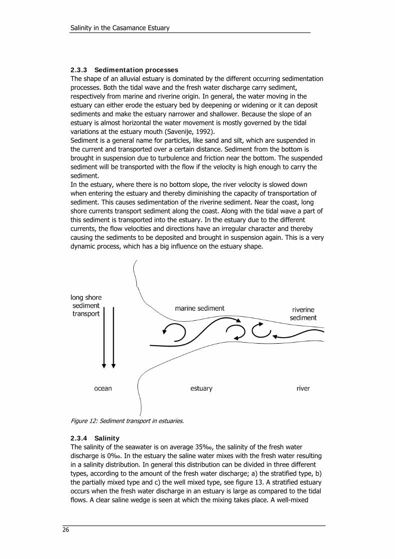
2.3.3 Sedimentation processes The shape of an alluvial estuary is dominated by the different occurring sedimentation processes. Both the tidal wave and the fresh water discharge carry sediment, respectively from marine and riverine origin. In general, the water moving in the estuary can either erode the estuary bed by deepening or widening or it can deposit sediments and make the estuary narrower and shallower. Because the slope of an estuary is almost horizontal the water movement is mostly governed by the tidal variations at the estuary mouth (Savenije, 1992). Sediment is a general name for particles, like sand and silt, which are suspended in the current and transported over a certain distance. Sediment from the bottom is brought in suspension due to turbulence and friction near the bottom. The suspended sediment will be transported with the flow if the velocity is high enough to carry the sediment. In the estuary, where there is no bottom slope, the river velocity is slowed down when entering the estuary and thereby diminishing the capacity of transportation of sediment. This causes sedimentation of the riverine sediment. Near the coast, long shore currents transport sediment along the coast. Along with the tidal wave a part of this sediment is transported into the estuary. In the estuary due to the different currents, the flow velocities and directions have an irregular character and thereby causing the sediments to be deposited and brought in suspension again. This is a very dynamic process, which has a big influence on the estuary shape.
Figure 12: Sediment transport in estuaries. 2.3.4 Salinity The salinity of the seawater is on average 35‰, the salinity of the fresh water discharge is 0‰. In the estuary the saline water mixes with the fresh water resulting in a salinity distribution. In general this distribution can be divided in three different types, according to the amount of the fresh water discharge; a) the stratified type, b) the partially mixed type and c) the well mixed type, see figure 13. A stratified estuary occurs when the fresh water discharge in an estuary is large as compared to the tidal flows. A clear saline wedge is seen at which the mixing takes place. A well-mixed

Occurrence and Consequences
27
estuary occurs when the fresh water discharge is small compared to the tidal flows. The salinity gradually changes over the estuary and the salinity distribution over depth is considered uniform. A partially mixed estuary has a distribution between these two extremes (Savenije, 2005).
1. The recession shape, which is found in narrow estuaries with a near-prismatic shape and a high river discharge.
2. The bell-shape, which occurs in estuaries that have a trumpet shape. That means these have a long convergence length in the upstream part, but a short convergence length near the mouth.
3. The dome shape, which occurs in strong funnel-shaped estuaries with a short convergence length.
4. The humpback shape, which is a negative or hypersaline estuary. (Savenije, 2005)
Figure 13: Three types of stratification in estuaries with a) the stratified type, b) the partially mixed type and c) the well mixed type.

Salinity in the Casamance Estuary
28
Figure 14: Salinity distributions along the estuary. 2.3.5 Hypersalinity The salinity distribution type 4 of figure 14 is of a hypersaline estuary; upstream of the estuary mouth higher salinity concentrations are found than the seawater salinity. The salt concentration at a point in the estuary is influenced by the supply of salt with the saline tidal wave, the evaporation of water in the estuary and the supply of fresh water. When in the dry season the evaporation exceeds the fresh water discharge, salt is stored in the estuary, usually far upstream of the estuary mouth. In the rainy season the fresh water discharge is higher than the evaporation and thereby transporting the stored salt downstream. If the annual fresh water discharge is not enough to flush the estuary, a yearly net accumulation of salt occurs. After a number of consecutive years of salt accumulation the estuary turns into a hypersaline estuary. When looking at this process, the only way to make a hypersaline estuary normal again is to “flush the toilet”. This can be done in one year with heavy rainfall, or in several consecutive years of high precipitation, that at the end of the rainy season no salt is left in the estuary, just like flushing the toilet. The salt concentration curve changes through the year, see figure 15, depending on the process described above, where at the end of the dry season a higher salinity is found further upstream than at the end of the rainy season, see figure 15. The transformation of a normal estuary into a hypersaline estuary has a big influence on the flora and fauna, because the present plants can’t cope with the high salt concentrations and die, leaving dead mud flats behind.

Occurrence and Consequences
29
Figure 15: Variation of the salinity distribution curve during the rainy season (modelled). In case of the Casamance the process of salinisation started with the Sahelian drought, which occurred in the late seventies, to turn the Casamance in a hypersaline estuary. Since the end of the Sahelian drought the rainfall has increased a bit, but hasn’t been able to “flush the toilet”. At the moment the Casamance still is a hypersaline estuary. The highest salt concentration measured in the Casamance was 188 kg/m3 on the 15th of May 1992 at 223 km from the estuary mouth (Thiam et al., 1998). The maximum salinity which can be reached is saturation level, 363 kg/m3 at 20°C. 2.3.6 Classification of estuaries A classification of estuaries is given in table 1. The Estuarine Richardson Number gives an indication of the salinity distribution of the estuary and is defined as the ratio of potential energy provided to the estuary by the river discharge through buoyancy of fresh water and the kinetic energy provided by the tide during a tidal period. If the Estuarine Richardson number is high, there is enough potential energy available in the river discharge to maintain a stratified estuary. If, on the other hand, the number is low, the kinetic energy available in the tidal currents is enough to mix the river water with saline water and the estuary is well mixed (Savenije, 2005). A ria is a submergent coastal landform, often known as a drowned valley of drowned river valley. Rias are usually formed when sea level rise or plate tectonics cause coastal levels to fall. When this happens, valleys which were previously at sea level become submerged. In rias no stage of morphological equilibrium has been reached yet, because the geological formation process is too fast for the sediment to keep up (Savenije, 2005).

Salinity in the Casamance Estuary
30
Shape Tidal wave typeRiver influence Geology Salinity
Estuarine Richardson Number
Bay Standing wave No river discharge
- Sea salinity Zero
Ria Mixed wave Small river discharge
Drowned drainage system
High salinity, often hypersaline
Small
Fjord Mixed wave Modest river discharge
Drowned glacier valley
Partially mixed to stratified
High
Funnel Mixed wave, large tidal range
Seasonal discharge
Alluvial in coastal plain
Well mixed Low
Delta Mixed wave, small tidal range
Seasonal discharge
Alluvial in coastal plain
Partially mixed Medium
Infinite prismatic channel
Progressive wave Seasonal discharge
Man-made Partially mixed to stratified
High
Table 1: Estuary classification with relation to tidal wave type, river influence, geology, salinity and estuary number (Savenije, 2005).

Occurrence and Consequences
31
2.3.7 The Casamance Estuary When looking at the estuary classification of table 1 the Casamance estuary has both characteristics of a ria as a funnel shaped estuary, namely a mixed tidal wave, small and seasonal river discharge, a hypersaline distribution which implicates a well-mixed estuary and a low Estuarine Richardson Number. An explanation for this can be that the Casamance has a ria shape which is slowly transforming into a funnel shape due to the strong sedimentation processes. This can be concluded from the genesis of the Casamance. The narrowing parts at the estuary mouth and near Ziguinchor are built up more recently according to Vieillefon (1997), see also figure 16. The sediment transported into the estuary from the seaside is deposited mostly in the mangrove zone. Due to the sedimentation the mangrove fall out of the reach of the water in the estuary, after which they expand further to the river reach and leave new gained land behind. This is an important explanation of the erratic shape of the river upstream of Ziguinchor. In the figure, also the old dunes around the estuary mouth can be seen, the strip on which Oussouye is located. From this figure a careful conclusion can be made that the strip in front of the old dunes was deposited while the estuary shifted along the coast. The silting up of the Casamance is nowadays a quite rapid process as can be seen from figure 17.
Figure 16: Recent and developed mangroves and ancient grounds (Vieillefon, 1977).

Salinity in the Casamance Estuary
32
Figure 17: Silting up near Ziguinchor: Iles aux Oiseaux (Vieillefon, 1977).

Occurrence and Consequences
33
3 Characteristics of the Casamance estuary
The system of the Casamance is mainly dominated by the tide and the salt intrusion. To describe these processes, the main features that influence these two processes have to be analysed first. All processes that occur in the estuary have their own time and length scales. Because of these scaling differences in two dimensions, it is hard to determine their relative influence. Besides a time and length scale, each process is also distinguished by a variance of its occurrence. To cope with these scaling differences is one of the major challenges of modelling. An overview of all processes and an indication of their time and length scales and their variance of occurrence are given in paragraph 3.1. There is a large interaction between the bathymetry and the processes that shape it, therefore the bathymetry will be described in paragraph 3.2. In the next paragraph the tidal parameters will be discussed more thoroughly in paragraph 3.3, following on the introduction made in the project area description. Rainfall, runoff and evaporation will be treated in paragraph 3.4. Salt intrusion is driven by mixing, an overview of the mixing processes and their importance in the Casamance is given in paragraph 3.5. To predict the salinity distribution, one of the main goals of the research, a simplification of the characteristics is needed so that they can be implemented in a predictive model. The simplifications of the bathymetry, tidal parameters and hydrological parameters will be described in these paragraphs. Other parameters, their sensitivity and the theoretical working of the model will be described in paragraph 3.6. Predictions on salinity distribution are done on basis of scenarios for the dominating processes. Processes that dominate in this scope are these processes that have a significant influence on discharge. This fact results in several scenarios on rainfall and runoff. The different scenarios and their outcome will be discussed in paragraph 3.7.

Salinity in the Casamance Estuary
34
3.1 Processes in the Casamance estuary
A process is here defined as an event that influences the water or salt balance in the estuary. Each process has its own time scale, length scale and variance, which are parameters that give an indication of their influence on the estuary. The occurrence of a process results in the estuary in the form of mixing and / or a water flow, but also has effects on other processes to occur in the estuary or not. The bathymetry of the estuary is under continuous influence of the water movement in the estuary, due to the erosion and sedimentation processes. The mixing, water flow and shape finally determine the salt intrusion, the final interest. This is schematised in figure 18. Internal represents the estuary which is under influence of its surroundings, external.
Figure 18: Schematisation of the estuary.
Overview of processes
The time and length scale and the variance give an approximation of the impact that the process has on the catchment, in other words the amount of discharge or mixing that occurs. In table 2 an attempt is made to list all processes, sorted on time scale. For all processes an indication is given of the variance and the resulting discharge and mixing. However the table lacks a considerable amount of data and knowledge, it is a good general overview and gives an insight in the complexity of the estuary before it is modelled.

Occurrence and Consequences
35
process timescale lengthscale variance water flow mixing
windwave 10 sec 10 m large
Hard to quantify, but when against flow direction important due to bar forming.
x = 100 m; y = 1 m wave / tide
shower 1 hour 5 km large 50 m3/s x = 5000 m; y = 2 m rainfall
wind upset 12 hours 50 km reasonable - x = 20000 m; y = 5 msalinity influence
semi diurnal tidal periodhalf lunar day 12:25
343 km insignificant 136 m3/s * x = 15000 m; y = 20 mbathymetry change
diurnal tidal period lunar day 24:50 higher order than estuary scale
insignificant 136 m3/s * x = 15000 m; y = 20 m evaporation
fresh water discharge surface runoff 2 days 50 km large 20 m3/s x = 5000 m; y = 2 m
flushing fields 2 days - large 20 m3/s x = 5000 m; y = 2 m
fortnightly tidal spring - neap variation 327:51 hours **higher order than estuary scale
minor ***
Discharge (storage) with in this period exists, hard to quantify.
Mixing with this period exists, hard to quantify
raining season 4 monthshigher order than estuary scale
large large variation x = 100000 m; y = 5 m
stable seasonal salt replacement 1 year estuary reasonable - x = 100000 m; y = 5 m
change of cross section mouth 1 year 100 m moderate influence influence
change of ocean salinity 1 year - insignificant - -
variation of mean sealevel 1 year mouth insignificantHard to quantify, but significant.
-
sedimentation of estuary long term estuary minor influence influence
evaporation constant catchment reasonable -27m3/s **** -
* (Brunet Moret, 1970)
** (Stewart, 2006)
*** yearly vatiation with maximum at the equinoxes
**** yearly average, calculated for total open water surface Table 2: Indication of different processes and their order of magnitude in the Casamance estuary.

Salinity in the Casamance Estuary
36
3.2 Bathymetry
The bathymetry contains the physical boundaries of the estuary, which is the most important characteristic of the estuary. The Casamance has a more complicated shape then the normal funnel shape of an estuary, which makes it more vulnerable for hypersalinity. 3.2.1 General shape of the Casamance The estuary of the Casamance consists of one main course, the Casamance river, with many branches. The main course reaches about 270 kilometres from west to east. The main course consists of an ebb channel surrounded by a lot of sand/mud banks which fall dry with ebb, or have a depth of a few meters with ebb. The zone between the water channels and land is covered with mangrove. The width of the strip of mangrove varies continuously along the estuary and also changes in density and type of mangrove. The geometry can basically be described as the following. The mouth is defined between Pointe De Diogué and Pointe De Nikine, but it is seen on the hydrographic map of C-Map (1996) that an important sand bank is situated at about 5 kilometres out of the defined mouth after which the depth increases to the mouth of the estuary. After the narrow mouth the main course widens rapidly, after which the estuary starts to narrow slowly, while several branches split from the main channel, until Ziguinchor. One important branch is the Diouloulou, which also has an other connection with the ocean. The land in this first part around the main course is dominated by several tributaries, with its banks filled with mangrove and swamp. On the land behind the mangrove, rice is cultivated. Directly upstream of Ziguinchor the main course widens very rapidly over a short distance and then has an erratically shape until Douma, in which it widens and narrows several times. The depth also makes a jump near Adéane at the point where the last large branch, the Soungrougrou, splits from the main course. At the widening upstream of Douma the channel forms a funnel shape till the end of the estuary. This is the part where the highest salt concentrations have been measured. 3.2.2 Theoretical description of the bathymetry There are three parameters that define the bathymetry in a point in a stream, the width, the cross section and the depth. The indication of the location is given in meters upstream from the mouth, the length determined by following the middle of the stream. According to Savenije (2005) energy is linearly dissipated along an estuary with a funnel shape, due to entropy. Therefore the cross section and width are expected to decrease exponentially with the distance. To evaluate this on the Casamance, the following formulas have been used on the estuary: ; (3.1) In these formulas a and b represent the convergence lengths of respectively the width and the cross section. Given the initial width (B0) and cross section (A0), the convergence lengths can be calculated with:
0
xB B exp
b⎛ ⎞= −⎜ ⎟⎝ ⎠ 0
xA A exp
a⎛ ⎞= −⎜ ⎟⎝ ⎠

Occurrence and Consequences
37
; (3.2) The shape of the estuary can be described with a convergence length (a, b), or, due to irregularities along the stream by more convergence lengths. To investigate whether irregularities in the Casamance occur, first the width and the cross section have been plotted exponentially in figure 19. The dots in the graphs represent all available data on bathymetry of the Casamance of the measurements of Debenay (1984, 1986), the information from the hydrological chart (C-map, 1996) over the first 60 kilometres (plotted as reaches60) and our own measurements, see appendix II. The graphs are plotted on a logarithmic scale, since exponential series should then transform to a linear course. Because the Casamance is morphologically not in equilibrium (see chapter 2) the ideal estuary shape is not (yet) reached and therefore many irregularities exist.
Width and cross section
1
10
100
1000
10000
100000
0 50 100 150 200 250
distance upstream (km)
Res
p. w
idth
(m
) an
d cr
oss
sect
ion
(m2)
Debenay widthWidth reaches60Measured widths IMeasured widths IIDebenay cross sectionCross section reaches60Measured cross sections IMeasured cross sections II
Figure 19: Width and cross section.
0
xb
ln(B /B )= −
( )0
xa
ln A / A= −

Salinity in the Casamance Estuary
38
At first the width is considered. From figure 19 can be seen that starting at the mouth the stream widens rapidly for the first kilometres and then it behaves purely exponential until 60 kilometres upstream, which is at Ziguinchor. After Ziguinchor, the stream widens rapidly, and because of the erratic shape, it’s hard to define the behaviour from merely some measurements. When looking at the cross section, one can again see an exponential start until 60 kilometres upstream, from this point, again an erratic shape with few measurements can be seen. The depth is not supposed to behave exponential and is therefore not plotted on logarithmic scale in figure 20. In contrast to the width and cross section, the depth behaves very erratically on the first 60 kilometres. From this point, a slow decrease in depth can be seen.
Depth
0
2
4
6
8
10
12
14
16
18
0 10 20 30 40 50 60 70 80 90 100
110
120
130
140
150
160
170
180
190
200
210
220
Distance upstream (km)
Dep
th (
m) Depth Debenay
Depth reaches60Measured depth IMeasured depth I
Figure 20: Depth h. 3.2.3 Description of bathymetry for the salt intrusion model The salt intrusion model divides the stream in reaches over which convergence lengths are constant. The original salt intrusion model (Savenije, 1990) can cope with four reaches with different convergence lengths. Choosing the ideal number of reaches to model the estuary is choosing between simplification and accuracy. The Casamance narrows and widens, over a lot of different length scales, and it’s hard to define which accuracy is significant to model and which not. This can only be done by trial and error. With calculations from the available bathymetry data, an ideal model can be made for any number of reaches. Here the final decision is made to divide the stream in six reaches, to model all dominant changes in the shape as described before, see figure 21. The result is shown in figure 22 and 23. In these graphs the models of total model describe the bathymetry in the model.

Occurrence and Consequences
39
Figure 21: Estuary shape of the Casamance
Width and cross section
1
10
100
1000
10000
100000
0 20 40 60 75 90 110
130
150
170
190
210
distance upstream (km)
Res
p. w
idth
(m
) an
d cr
oss
sect
ion
(m2)
Width total modelDebenay widthWidth reaches60Cross sesction total modelDebenay cross sectionCross section reaches60
Figure 22: Width and cross section.

Salinity in the Casamance Estuary
40
Depth
0
2
4
6
8
10
12
14
16
180 10 20 30 40 50 60 70 80 90 100
110
120
130
140
150
160
170
180
190
200
210
220
Distance upstream (km)
Dep
th (
m)
Depth Total ModelDepth DebenayDepth reaches60
Figure 23: Depth h.

Occurrence and Consequences
41
3.3 Tidal parameters
To describe the tidal propagation in the estuary, several parameters have to be defined. In this paragraph, each parameter’s definition is given and its values and behaviour for the Casamance. From paragraph 3.3.1 until 3.4.5 all parameters will be described. In subparagraph 3.6 the implementation in the salt intrusion model will be described. 3.3.1 Tidal range The tidal range (H) is the difference between the ebb and flood level. The tidal range varies in time between spring- and neap tide and with the diurnal inequality. Further upstream in the estuary the range is damped. At the estuary mouth, according to TotalTideTM, the tidal range at Pointe Diogué differs from 1.6 m to 1.5 m during springtide (due to diurnal inequality) and from 0.6 m to 0.4 m during neap tide. The 27-09-2006 measurements at Karabane (near the estuary mouth) also showed a range of 1.6 m during springtide, see appendix II. 3.3.2 Tidal reach The tide propagates into the estuary until Diana Malary, which lays 240 kilometres upstream from the mouth and around 30 kilometres downstream of Kolda. Due to estuary level differences in the rainy season and the annual variability of the mean sea level this point is not constant. During low level at either sea or estuary, the tide propagates less far. Since the tidal wave velocity is in the order of 3.5 m/s in the estuary (more or less representative for the whole estuary, 20-09-2006 measurements), the consequence of a tidal reach of 240000 meter is a travel time of 68571 sec. Since the tidal period is only 44700 sec, there are continuously 1.5 tidal waves in the estuary. In other words when it’s flood at Pointe de Diogué it is flood at Goudomp and ebb at Diana Malary. 3.3.3 Tidal damping The tidal damping (∂) is a measure for the decrease of the tidal range along the estuary. The tidal range decreases exponentially due to friction, as the tide propagates upstream in the estuary. To receive custom values, and because the salt intrusion model is set that way, the tidal damping is here expressed in damping per 5 kilometres. The damping term used in the model is the tidal damping to the power of the length between two points along the stream (divided by 5000 m), if multiplied with the downstream tidal range delivers the upstream tidal range.
∂i L2 1H =H (3.3)
For determining the tidal damping, different sources can be used. During the 20-9-2006 measurements the tidal range was measured at respectively Ziguinchor, Goudomp and Sedhiou, see appendix II. These measurements resulted in a tidal damping for the trace Ziguinchor – Goudomp of 0.907 (per 5000 m) and for the trace Goudomp – Sedhiou of 0.987. Combination of the 09-09-2006 springtide measurement at Ziguinchor and the 27-09-2006 springtide measurement at Karabane resulted in a tidal damping of 0.922 (per 5000 m). With the information of Génie Rurale of the water stage in Goudomp and Ziguinchor it is possible to determine the damping between Ziguinchor and Goudomp. The stage

Salinity in the Casamance Estuary
42
data of the year 2001 is most useful, because measurements were done several times a day. In Ziguinchor more than 20 measurements were done a day and in Goudomp usually around 15 measurements were done a day. Because so many data is available from the water level, the extremes of the tidal cycles are easily defined. In other years and at other locations measurements were done less frequently. These data are less useful because the time of a HW or a LW is easily missed. The tide from 2 till 4 February of 2001 in Ziguinchor and Goudomp is plotted in figure 24. It can be seen that the tidal range in Ziguinchor is larger than in Goudomp. According to the water height measurements in 2001 the tidal range in Ziguinchor is on average 60.7 cm and 18.4 cm in Goudomp. This results in an average damping of 0.885 (per 5000 m). There is almost no difference between the damping in the rainy and the dry season.
Water Stage 2-4 February 2001(Relative to ML)
-40
-30
-20
-10
0
10
20
30
40
2-02
-01
0:00
2-02
-01
1:30
2-02
-01
3:00
2-02
-01
4:30
2-02
-01
6:00
2-02
-01
7:30
2-02
-01
9:00
2-02
-01
10:3
02-
02-0
1 12
:00
2-02
-01
13:3
02-
02-0
1 15
:00
2-02
-01
16:3
02-
02-0
1 18
:00
2-02
-01
19:3
02-
02-0
1 21
:00
2-02
-01
22:3
03-
02-0
1 0:
003-
02-0
1 1:
303-
02-0
1 3:
003-
02-0
1 4:
303-
02-0
1 6:
003-
02-0
1 7:
303-
02-0
1 9:
003-
02-0
1 10
:30
3-02
-01
12:0
03-
02-0
1 13
:30
3-02
-01
15:0
03-
02-0
1 16
:30
3-02
-01
18:0
03-
02-0
1 19
:30
3-02
-01
21:0
03-
02-0
1 22
:30
4-02
-01
0:00
4-02
-01
1:30
4-02
-01
3:00
4-02
-01
4:30
4-02
-01
6:00
4-02
-01
7:30
4-02
-01
9:00
4-02
-01
10:3
04-
02-0
1 12
:00
Date
Hei
ght (c
m)
Water Height Ziguinchor
Water Height Goudomp
Figure 24: Water level in the Casamance at Ziguinchor and Goudomp (Génie Rurale) From the plot of Brunet – Moret 1970 a tidal damping of 0.94 (per 5000 m) can be determined over the first 75 kilometres of the stream. Over 200 kilometres a damping of 0.90 (per 5000 m) is determined. Besides that, from the figure can be seen that the tidal amplitude indeed decreases exponentially. In this figure the spring tide amplitude is also plotted, this gives the same values for tidal damping over 75 and 200 kilometres, so the damping is independent of the tidal range, which justifies comparing different measurements. Of the above calculations, finally a damping of 0.91 is chosen. If with this damping factor the tidal range is calculated at Diana Malary, the tidal reach, a tidal range of 0.017 m is found. This is a satisfying result, since theoretically the tidal range should be zero. It can be said that the tidal damping is independent on the tidal range and that damping in the estuary is not constant but exponential.

Occurrence and Consequences
43
3.3.4 Phase lag The phase lag (ε) is the time between HW and HWS (or LW and LWS). Theoretically, it is the shift that is made between the graph of the height and the velocity. The phase lag in an alluvial estuary lies between 0 and ½ π. For estuaries where the tidal range is damped or amplified the phase lag is not constant along the estuary. As in the Casamance the tidal range is damped, the phase lag is not constant. The phase lag can simply be determined by measuring the time between HW and HWS (but preferably between LW and LWS, since LW time is easier to determine). It is also possible to derive the phase lag from the tidal range and the range of the slack moments with: rewritten to: (3.4) In which H is the tidal range, H’ is the tidal range between the HWS and LWS and ε is the phase lag (Savenije, 2005). From the 09-09-2006 measurements at Ziguinchor this H and H’ can be derived, which are respectively 0.585 m and 0.075 m. This results in a phase lag ε of 1.442 or 0.459 π. This value is close to ½ π which is the phase lag in a prismatic channel. However the convergence length of the river bends at Ziguinchor is quite large, the channel cannot be considered as prismatic, which makes the value unrealistic. An explanation for this can be found in the accuracy of the measurements. The measured tidal range of the slack moments, 0.075 m, is in the order of the measuring order and thus by using this number a value is calculated with a big uncertainty. Therefore it is not possible to use this formula on the Casamance estuary. During the 20-09-2006 measurements a phase lag of 2 hours was measured at Ziguinchor (63 kilometres from mouth), 1.5 hours at Goudomp (at 112 km) and an hour at Sedhiou (at 170 km). From these measurements a linear decrease can be derived. This however cannot occur on the whole estuary because if this is linearly extrapolated to the mouth, a phase lag of 0.4 π is found, where it should be near 0, since the pure tidal wave is a standing wave. The behaviour of the phase lag is hard to define, there are too few measurements, and the shape of the estuary is too irregular to determine a relation for the phase lag. 3.3.5 Tidal prism The tidal prism (Pt) or flood volume is the volume of water entering the estuary at the mouth between HWS and LWS. With the bathymetry defined in paragraph 3.2 it is possible to define the tidal prism in combination with the tidal damping (∂), the tidal range at the mouth (H0) and O: (3.5) Since the phase lag at the mouth can be considered near 0, the flood volume can be defined as 0.331*109 m2.
( )0t
H
H OP cos
1 b= ε
− ∂
= εH' Hcos −ε = 1 H'cos ( )
H

Salinity in the Casamance Estuary
44
3.3.6 Tidal excursion The tidal excursion (E) is the total distance travelled by a water particle that is floating in the estuary during one tidal cycle. The tidal excursion is a measure to determine the dispersion. Assume that there is no fresh water discharge and no evaporation, then the water particle will return to the same place when the tidal cycle is finished. With the measured velocity amplitude at the surface of 1.06 m/s during the 09-09-2006 measurement and the period of the tidal wave of 44700 sec the tidal excursion can be determined with:
υω2
E= with: πω 2
=T
(3.6)
This results in a tidal excursion of 15076.63 m. With the tidal prism calculated in the previous section, the tidal excursion can be calculated: rewritten to: (3.7) This results in a value of 15045.45 m, which is very well comparable with the measured result. 3.3.7 Spring - neap variation During research for a stage – discharge relation with the water heights of Ziguinchor and Goudomp series of Genie Rurale Ziguinchor the semi-diurnal tide was filtered out by computing the average water height over the two high waters and two low waters. The average water heights now depend only on annual mean sea level variation and amounts of rainfall water that enter the Casamance estuary. In figure 25 the water levels relative to their ML are plotted for the period end-January till mid-October of the year 2001. Because the shape of both graphs is almost similar, it can be concluded that both measurements were done correctly and the data are reliable.
Stage Ziguinchor and Goudomp in 2001(Relative to ML)
-25-20-15-10-505
1015202530
9-1 29-1 18-2 10-3 30-3 19-4 9-5 29-5 18-6 8-7 28-7 17-8 6-9 26-9 16-10 5-11
Date (dd:mm)
Stag
e (c
m)
ZiguinchorGoudomp
Figure 25: Water levels in Ziguinchor and Goudomp in 2001.
t 0 0P A E= t0
0
PE
A=

Occurrence and Consequences
45
Immediately can be seen from the plot, that before the rainy season starts an irregularity in the water level occurs which is not caused by runoff and neither by annual mean sea level variation. The period of this irregularity is exactly lunar, so due to spring neap variation. Because during spring tide only the amplitude changes, and not the whole sea level, this effect must have been filtered out with the semidiurnal tide. The only explanation for the periodic changes in water level as measured is that during springtide a significant amount of water is stored in the estuary, which flows out during neap tide, causing the variation. Because of the large amount of surface with mudflats and mangrove, this is considered as possible. This ‘fortnightly tidal prism’ will have a height of 0 m at the mouth, but will grow further upstream. The amplitude at Ziguinchor and Goudomp is about 0.10 m. The exact tidal prism of this movement is hard to define, but this prism will result in a fortnightly tidal excursion in the order of 2 kilometres (derived with the formulas under tidal excursion) and is therefore significant. 3.3.8 Tidal parameters in the salt intrusion model In the model, a few tidal parameters are described. Besides the tidal period (44700 sec) the average tidal range and the tidal damping are used. The average tidal range is defined as the average of a spring tide and a neap tide at Pointe Diogué, which are defined out of the average of both diurnal tides. An average range of 1.02 metre is then obtained. For the tidal damping 0.91 over 500 metres is chosen, based on the measurements above.

Salinity in the Casamance Estuary
46
3.4 Hydrological parameters
The hydrological parameters are described in this paragraph. Monthly aerial rainfall, open water evaporation and fresh water discharge are important input parameters for the salt intrusion model as these vary widely over time and space. Stating that the tidal influence and estuary bathymetry can be considered as constant over the recent history, only these hydrological parameters remain to determine the salt distribution through the estuary; the main external processes. The aerial rainfall will be calculated, as well as an average monthly open water evaporation distribution. Then the measured discharges at a station upstream, with no tidal influence, will be discussed, followed by an analysis of the order of magnitude of the parameters and their consistency when used for a salt intrusion model. 3.4.1 Rainfall The rainfall is not evenly distributed over the Casamance basin. To estimate the average precipitation over the catchment a Thiessen polygon has been created for the basin. With the Thiessen method, lines are drawn to connect reliable rainfall stations. The connecting lines are bisected perpendicularly to form a polygon around each station. To determine the mean rainfall of the catchment, the rainfall amount of each station is multiplied by the area of its polygon and the sum of the products is divided by the total area. An example of a Thiessen Polygon is given in figure 26 (Savenije et al., 2006).
Figure 26: A Thiessen polygon for a certain area (Savenije et al., 2006) A total of nine stations has been used. From west to east these stations are Kabrousse, Loudia-Ouolof, Diouloulou, Bignona, Ziguinchor, Marsassoum, Sedhiou, Kolda and Velingara (which is situated outside the catchment). The catchment area with its Thiessen polygons is displayed in figure 27. Daily precipitation data from the period 1970 until 2004 is used from 8 stations; from the Kolda station only data was available from 2000 to 2004. Kolda is included in the Thiessen polygon because it is the only place between Sedhiou and Velingara, thus making the calculation of the average rainfall over the area more accurate. Therefore, two different Thiessen polygons are drawn; one for the period from 1970 until 1999 and one for the period from 2000 to 2004. This results in different dimensions of the

Occurrence and Consequences
47
sub-areas for these periods. The position of all the used rainfall stations and the accompanying areas can be seen in figure 27. The Thiessen polygon of figure 27 is the one that has been used for the period 2000 – 2004, which includes the area of Kolda.
Figure 27: Thiessen polygons, drawn over the Casamance Catchment, representing different rainfall measuring stations. Besides Kolda, there are 5 other stations with incomplete data. This varies from missing data of one year to 7 years. These missing data are estimated by filling them up with monthly average values from the neighbouring stations.
Average Precipitation Casamance Catchment and Ziguinchor 1970-2004
050
100150200250300350400450
Janu
ary
Febr
uary
Mar
ch
Apr
il
May
June
July
Aug
ust
Sept
embe
r
Oct
ober
Nov
embe
r
Dec
embe
r
Time (months)
Prec
ipita
tion
(mm
/mon
th)
Casamance CatchmentZiguinchor
Figure 28: Average precipitation of the Casamance catchment and Ziguinchor from the period 1970 until 2004. The average precipitation values of the Casamance catchment and at Ziguinchor from 1970 until 2004 are plotted in figure 28. In the month with the highest precipitation, August, the average rainfall in the catchment is 331.7 mm/month.

Salinity in the Casamance Estuary
48
In figure 28 can be seen that the precipitation in Ziguinchor in the period from 1970 until 2004 is on average higher than the average precipitation over the whole catchment over the same period. To estimate the precipitation of the catchment a correlation of the yearly precipitation Ziguinchor and the Casamance catchment is made, which is shown in figure 29.
Correlation Casamance Catchment and Ziguinchor on yearly data
y = 0,8818xR2 = 0,4885
0
200
400
600
800
1000
1200
1400
1600
1800
2000
0 200 400 600 800 1000 1200 1400 1600 1800 2000
Precipitation Ziguinchor (mm/y)
Prec
ipita
tion
Cas
aman
ce C
atch
men
t (m
m/y
)
Figure 29: Correlation diagram of yearly precipitation with the whole basin plotted against the rainfall in Ziguinchor. The average yearly precipitation of the catchment can be estimated by multiplying the yearly precipitation of Ziguinchor with -0.8818. This is not a good correlation however and it will not be used further on.

Occurrence and Consequences
49
3.4.2 Evaporation Evaporation is an important parameter in the salt intrusion model, because it determines the dilution in the dry season to a large extend. Especially further upstream, where the tidal mixing component is less evaporation is a key parameter in the salinisation process, as discussed in paragraph 2.3.4. Comments on previous modelled evapotranspiration In the old salt intrusion model that has been set up by Savenije in 1992, the potential evapotranspiration calculated with Penman’s formula, was used as input data. On basis of four years of measurements, an average yearly profile is derived as displayed in figure 30. These monthly averages are used as input data in the salt intrusion model, by creating a time series in which all years are equal.
FAO Climwat and empiric potential evapotranspiration
0
0.05
0.1
0.15
0.2
0.25
0.3
Janu
ary
Febr
uary
Mar
ch
April
May
June July
Augu
st
Sept
embe
r
Oct
ober
Nov
embe
r
Dec
embe
r
time (months)
ETo
(m/m
onth
)
FAO Climwatdatabase
average estimation1984-1988
Figure 30: Potential evapotranspiration in Ziguinchor as calculated by the FAO for the Climwat database and the average ETo values calculated by Savenije based on daily evaporation measurements from 1984 until 1988. The FAO provides global climate information for agriculture and has calculated the average monthly evapotranspiration as displayed in the figure above. On what measurements these values are based is not clear, but the difference with the estimated values in Ziguinchor is striking: 1856 mm/year according to FAO versus 1682 mm/y estimated by Savenije, the difference being more than 10 percent. Both distributions appear to agree on the evaporation in the rainy season, when humidity is the limiting parameter for evaporation. The dry season however, being far more interesting for salt intrusion modelling, is structurally higher according to the FAO’s calculations. They claim that potential evapotranspiration is equal in Kolda and Ziguinchor. Since the spatial variability in rainfall and temperature is rather large (and thus the humidity), one would expect a higher yearly evaporation in the upstream region. The Climwat data should thus merely be seen as an estimated aerial average

Salinity in the Casamance Estuary
50
for the catchment, which can be expected to be more than the measured evaporation in Ziguinchor. Open water evaporation versus evapotranspiration An important remark here is that open water evaporation is generally more than potential evapotranspiration (Savenijne et al. 2006) and completely different from evapotranspiration since there is no stomatal resistance and negligible aerodynamic resistance, while the reflection of radiation is little compared to most land and heat capacity completely different, causing that water does not heat up as easy as land. Since we are interested in the evaporation of the water in the estuary, we should look at open water evaporation. In the next paragraph an estimate of monthly open water evaporation will be derived. Salt water evaporation Last remark is the salinity of the water. Salt, when diluted, alters the vapour pressure and thus the heat capacity of water, resulting in a decreased evaporation rate of 1% for every 1% diluted salt (Ward et al., 2000). As salinity is variable over time and space in the estuary, the influence of this parameter on the open water evaporation is difficult to determine. When working with monthly averages the error introduced by neglecting these effects could be significant, since salinities of up to 17 percent occur. For our investigation however, this influence will be neglected, as other parameters are presumably even less accurately estimable and more significant.
Calculation of open water evaporation
When estimating evaporation with Penmans equation, wind, temperature, humidity and radiation are the atmospheric parameters that determine the open water evaporation rate. The geometry of the water body itself is important as well, as a shallow basin will heat up quicker than a deeper one with the same volume and has a relatively larger surface from where water can evaporate. Hence it is clear that the yearly evaporation varies spatially and in time. But, with reliable evaporation data being very scarce, variability is difficult to take into account. The difference between measured series is considerably large and correlation with more reliable data such as measured precipitation appears to be nil, which follows from the variability in other key parameters. Open water evaporation will be calculated here with Penmans evaporation model, thus neglecting the water body characteristics as geometry and salinity and reducing the atmospheric parameters of influence to wind, radiation, temperature and humidity. For Ziguinchor average monthly data for wind, temperature and humidity are available. FAO calculates the aerial average on basis of more wind and less humidity than measured in Ziguinchor, but in general these data correspond satisfactory. Radiation data provided by the FAO differs much from the estimate based on latitude provided by the hydrology lecture notes (Savenije et al., 2006). For the calculation the hours of sunshine, n, provided by the FAO will be combined with the tabulated maximum hours of sunshine in the area, N, and the average daily short wave radiation per surface area RA. The input parameters are summarized in table 3.

Occurrence and Consequences
51
maximum
temperature* minimum temperature*
wind speed*
humidity* sunshine* maximum hours sunshine**
short wave radiation**
month (°C) (°C) (m/s) (%) (hours) (hours) (J d-1m-2)
January 35 15.8 2.199 61 6.7 11.45 28052500
February 35.5 16 2.801 64 8 11.7 28665000
March 37 17 2.905 65 9.3 12 29400000
April 37.2 18.6 3.495 66 9.8 12.4 30380000
May 35.6 20.7 3.704 73 8.7 12.7 31115000
June 33.8 22.8 2.998 77 5.6 12.85 31482500
July 31.6 23 2.801 83 3.9 12.75 31237500
August 30.6 22.8 2.604 85 3 12.5 30625000
September 31.2 22.5 2.199 87 5.1 12.15 29767500
October 32.7 22.5 1.898 85 6.6 12 29400000
November 33.3 20 1.898 86 7.8 11.5 28175000
December 32.6 17.5 2.002 71 5.6 11.35 27807500
Table 3: Input data for calculation open water evaporation. * Monthly averages from FAO climwat database ** Monthly calculated on basis of latitude presented in hydrology 1 Net radiation, RN will be calculated with the balance:
1 2N C C B C BR R rR R (1 r)R R Jd m− −⎡ ⎤= − − = − − ⎣ ⎦ (3.8)
For the net short wave radiation that heats up the earth’s surface the short wave fraction that reaches the earth has to be diminished by the reflected short wave radiation, wherefore the empirical formula is used with a- and b-coefficients for an average climate being 0.25 and 0.50 (Savenije, 2006).
1 2C a
nR (a b )R Jd m
N− −⎡ ⎤= + ⎣ ⎦ (3.9)
Much of this energy will disappear from the surface as long wave radiation, RB. This can be estimated with the formula below, using the actual vapour pressure ea and the actual air temperature ta in relation with the fraction of the available hours of sunshine that reaches the earth n/N.
4 1 2B a a
nR (273 t ) (0.47 0.21 e )(0.2 0.8 ) Jd m
N− −⎡ ⎤= σ + − + ⎣ ⎦ (3.10)
For the actual temperature the mean of the maximum temperature tmax and minimum temperature tmin has been taken, while the actual vapour pressure calculated as the average of the ea,min calculated on basis of the relative humidity times es at tmin and ea,max for tmax. Since this averaging introduces many errors (monthly average temperature is not the mean of its maximum and minimum values), with especially the temperature term being important, it is clear that the total long wave radiation can only be roughly estimated. The same goes for the hours of sunshine, n, which may vary a lot. Hence the uncertainty in the net radiation is large. Luckily the radiation term in Penmans evaporation model is small, compared to the right hand term in equation 3.8. The parameters and coefficients are explained in the table below.

Salinity in the Casamance Estuary
52
p a a aN
a 10
c (e e )sRr
E mds
−
ρ⎧ ⎫−+⎨ ⎬ρλ ρλ⎩ ⎭ ⎡ ⎤= ⎣ ⎦+ γ
(3.11)
parameter symbol constant unit specific heat of air by constant pressure cp 1004 J kg-1 K-1 latent heat of vaporization λ 2450000 J kg-1 mean air density at constant pressure ρa 1.205 kg m-3 mean density of fresh water at constant pressure ρ 1000 kg m-3 psychrometric constant γ 0.066 kPa °C-1 Angström coefficient a a 0.25 - Angström coefficient b b 0.5 - Stefan-Boltzmann constant σ 4.90 *10-3 J d-1m-2 oK-4 albedo open water r 0.06 - slope of vapour pressure curve at
s kPa °C-1
saturation vapour pressure es kPa actual vapour pressure ea kPa aerodynamic resistance ra s m-1
Table 4: Parameters and coefficients used with Penmans evaporation model. sRN is at least twice as small as the wind-temperature-humidity term and about ten times smaller at the end of the dry season. As the these terms vary the most through the year, with the radiation being relatively constant through the year in this area of the world, the evaporation pattern can be said to be largely dependent on these climatic parameters. When calculating the yearly evaporation rate with various measured monthly averages for humidity, temperature and wind, one would find differences smaller than 10%. This sufficiently justifies the usage of the average yearly evaporation in the salt intrusion model, as the order of magnitude will not be affected by altering climate conditions. The average monthly evaporation depths for the basin are displayed in table 5 and the average climatic conditions are summarized in figure 31. The yearly rate is about 2000 mm, which is relatively normal for the tropic climate conditions (Savenije, 2006).

Occurrence and Consequences
53
month open water evaporation Eo
mm/month January 163 February 177 March 227 April 237 May 221 June 165 July 141 August 128 September 142 October 161 November 156 December 137 yearly total 2056 Table 5: Average monthly open water evaporation rate from Penman model based on estimated average climate condition in the Casamance basin.
average climate data Casamance basin
0
10
20
30
40
50
60
70
80
90
100
Janu
ary
Febr
uary
Mar
ch
April
May
June July
Augu
st
Sept
embe
r
Oct
ober
Nov
embe
r
Dec
embe
r
month
tem
pera
ture
(de
gree
s C)
/ re
lativ
e hu
mid
ity (
%)
0
40
80
120
160
200
240
280
320
360
400
evap
orat
ion
(mm
/mth
)/
rain
fall
(mm
/mth
)
temperaturerange ( degreeCelsius)humidity (%)
rainfall(mm/mth)
open waterevaporation Eo(mm/mth)
Figure 31: Climate data from table 4 and 5 represented in a graph. Figure 31 is significantly different from figure 6 represented in chapter 1, showing the temperature, evaporation and rainfall in Ziguinchor. Here one sees clearly how humidity is high in the rainy season, with a corresponding low evaporation rate. Average temperature does not change much over the year, but the range is significantly wider in the dryer months, thus making it necessary to use minimum and maximum values when calculating vapour pressure.

Salinity in the Casamance Estuary
54
3.4.3 Runoff The last important hydrological parameter for the salt intrusion model is the runoff, i.e. the fresh water discharge to the estuary. Since it is difficult to measure the fresh water discharge directly in a basin with tidal influence, the only reliable discharge data provided are the series measured at Kolda, about 280 km upstream. This part of the estuary has negligible tidal influence and the river bed is dry most years from January till May. Water level is measured here daily and the matching discharge is measured a few times per year using various devices. The discharge is not regularly measured at high discharge which makes the series a bit unreliable at its maxima.
Figure 32: Water level measuring equipment at the bridge over the Casamance in Kolda. The devices do not work anymore, but nowadays the water level is measured everyday visually on a ruler nearby. For the model it is important to have an estimate of the monthly fresh water discharge at the estuary mouth, Q0. This is calculated on basis of the upstream incoming fresh water flux, by adding rainfall and subtracting evaporation proportionally to the open water area. Major drawback of this method is that freshwater discharge, Qf, is underestimated in the months without rainfall, since the incoming discharge from upstream can only be diminished by evaporation. One could estimate the fresh water discharge as well by multiplying the measured values at Kolda by the inverse of the relative size of the sub catchment, with Atot being the total catchment area in km2 and Ak its equivalent for the Kolda sub catchment (c.q. 20000 km2 and 3700 km2)
3tot0 k
k
AQ Q m /mth
A⎡ ⎤= ⎣ ⎦ (3.12)

Occurrence and Consequences
55
This seems a good estimate, as the Casamance basins geography is relative homogeneous and the westernmost part of the basin receives more rain, but drains directly to the ocean as well, via numerous small bolons at the north shore. However, an estimate of the discharge distribution at some point upstream remains necessary. As the measured series has some holes in the data (where no measurements where done). As a better insight in the drainage process is important when building realistic scenarios in rainfall and runoff, a rainfall-runoff relation is sought for.
Rainfall-runoff modelling through modelling
For various years the discharge at Kolda is measured. For the period 1965 until 1980 the rainfall is measured here as well. When the discharge integrated over time and divided by the catchment area, it can be easily compared with the rainfall since they both can be expressed in meters per month. After subtracting an initial interception loss of 50 mm/month, an estimate of the effective precipitation can be compared with discharge graphically as in figure 33.
rainfall-runoff relation 1965-1980
R2 = 0.6211
R2 = 0.0438
R2 = 0.4046
R2 = 0.1918
-0.015
-0.01
-0.005
0
0.005
0.01
0.015
0.02
0.025
0.03
0.035
0 0.1 0.2 0.3 0.4 0.5 0.6
effective precipitation (m/mth)
disc
harg
e (m
/mth
)
May
June
July
Aug
Sept
Oct
Nov
Dec
September
July
August
October
Figure 33: Effective monthly precipitation and discharge for the Kolda sub catchment for the period 1965 till 1980. The discharge appears to be at least ten times smaller than the rainfall, indicating a very low runoff coefficient, which is on a yearly basis about 2.5% (about 5% for wet years). Normally one could estimate the initial infiltration loss by drawing a trend line and find the intersection with the horizontal axis as the infiltration rate. For June and July, the beginning of the rainy season, there appears to be no loss, while for August

Salinity in the Casamance Estuary
56
and September, as the soil is expected to be saturated with water, the method seems to work. As the correlation factors show near the trend lines, error is rather large. In September for example we can find discharge of about 0.005 and 0.030 m/month with a rainfall of a little more than 400 mm/month. One could question the accuracy of both measured parameters, but it must be clear that there is no linear relation between monthly rainfall and runoff. This explains why simple linear regression methods do not work for the sub catchment. A similar plot with accumulated values for a hydrological year (from May until April), has a very low correlation as well, which supports this statement. Apparently processes in the sub catchment can not be described with simple methods. Another rainfall series for Kolda, starting in the year 2000, could be used as well. Due to some gaps in the discharge data, the rainfall-runoff series is diminished to 3 years. Not much for a thorough investigation. But from these series again it is clear that a clear relation between rainfall and runoff cannot easily be found. Figure 34 shows the rainfall in the hydrological years 2001-2004. Qcalc is the discharge calculated with a conceptual bucket or linear reservoir model, with basically two buckets (as discussed in the Hydrological Modelling course at TU Delft); the saturated zone and the unsaturated zone. There is no routing and the percolation rate and maximum soil moisture capacity are the main calibration parameters.
rain and runoff in Kolda subcatchment
0
0,1
0,2
0,3
0,4
0,5
0,6
May
-01
Jul-0
1
Sep-
01
Nov
-01
Jan-
02
Mar
-02
May
-02
Jul-0
2
Sep-
02
Nov
-02
Jan-
03
Mar
-03
May
-03
Jul-0
3
Sep-
03
Nov
-03
Jan-
04
Mar
-04
time (mth)
rain
fall
(m/m
th)
0
0,002
0,004
0,006
0,008
0,01
0,012
runo
ff (
m/m
th)
rain (m)
Q (m/mth)
Qcalc (m/mth)
Qregr (m/mth)
Figure 34: Rainfall and corresponding measured and simulated runoff in the Kolda sub catchment. Qcalc is simulated with a linear reservoir model. Qregr is modelled with a linear backward relation (Savenije, 2006). From the figure it is clear that the discharge distribution over the months cannot be estimated with these methods. Either the first year is wrong in maximum value and time of occurrence or the general simulated shape, or the last year does not match the measured discharges.

Occurrence and Consequences
57
For now it is clear that the relation between rainfall and runoff for the sub catchment is complex. Whether this is due to spatial variation in rainfall, inaccurate measurements or other factors cannot be said. There appears to be no choice but to fill the gaps in the data series by multiplying the average discharge distribution with the percentage deviation of the average yearly rainfall for that hydrological year. figure 34 showed that that linear interpolation lacks accuracy especially in wetter conditions, but there is no other choice. 3.4.4 Hydrological parameters in the salt intrusion model All hydrological input data can be found in appendix III. Here the techniques used to obtain them are summarized. parameter time line calculation method unit aerial rainfall 1970-2004 Thiessen polygon for 9
measuring stations m/mth
open water evaporation
monthly average per month
Penmans evaporation model
m/mth
upstream fresh water discharge
1970-2004 measured at Kolda, gaps filled with linear interpolation
m3/s average value per month
Table 6: Hydrological parameters with their calculation method. When averaging rainfall over the years one could calculate the average monthly volume of fresh water provided by rainfall in the estuary on the open water surface. The same goes for evaporation. The average measured monthly discharge in the Kolda catchment can be multiplied by 20000/3700 to get an extrapolated discharge distribution. These values can be used to calculate the freshwater available in the estuary for dilution by subtracting the evaporation from the sum of rainfall and discharge.
3f 0 0S P Q E m /mth⎡ ⎤= + − ⎣ ⎦ (3.13)
Sf is the ‘stored’ fresh water in the estuary. This sign of this balance chances over time; in the dry season water evaporates while there is negligible inflow from fresh water discharge. For a hydrological year the ‘stored’ fresh water volume can be accounted for, as displayed in figure 36. First remark here is that for both evaporation and rainfall, the volume is calculated on basis of the open water surface used in the salt intrusion model (with the convergence lengths, thus the stream width that has flow). This results in an underestimation, since the open water surface is much larger at times due to bank storage (like the tidal flats with mangroves). Rain that falls on the main course will become runoff and this leads to some double counting, which thus means an overestimate of the balance. This is rather small however. The salt intrusion model calculates the fresh water discharge at the estuary mouth by adding rainfall volume per month times a factor and subtracting evaporated volume per months times a factor, as discussed in paragraph 3.4.5. A factor of about 3.5 for rainfall gives a maximum Q0 that corresponds with the technique described above. The factor for the evaporation open water surface area remains arbitrary but must be smaller than 3.5

Salinity in the Casamance Estuary
58
since the open water surface available for evaporation is generally less (much land fall dry in the dry season when evaporation is the dominant term). Second remark is that not all runoff is stored. Much ‘fresh’ water discharge will leave the estuary as outflow at the mouth. This is another overestimation of the fresh water availability.
balance P-Q-Eo
-1.00E+08
-5.00E+07
0.00E+00
5.00E+07
1.00E+08
1.50E+08
May
June
July
Aug
Sept
Oct
Nov
Dec
Jan
Feb
Mar
Apr
time (mth)
flux
(m3/
mth
)
balance P+Q-E
rainfall(m3/mth)discharge Qo(m3/mth)evaporation(m3/mth)
yearly average fluxes in m3/year for the Casamance basin on basis of measured series 1970-2003 precipitation (P) discharge Q0 evaporation (E0) balance P+Q0-E0 2.95E+08 3.01E+08 5.84E+08 1.27E+07 Figure 35: Balance of fresh water on basis of average monthly rainfall, open water evaporation and fresh water discharge, calculated in this chapter. Below the yearly average volumes are presented for the basin. Whether these effects cancel each other out is not known. Figure 36 is calculated without any multiplication factors for rain and evaporation surface, but indicates how fragile the equilibrium is. The hatched area is the storage, which has positive part in the rainy season but becomes negative from November already. In the figure the net yearly storage of fresh water is about 1.3E+7, thus still positive. This should indicate that there should be net desalinisation in an ‘average year.’ Since the Casamance is hypersaline, this can not be the case. Either the rainfall/ evaporation ratio is underestimated, or the error introduced by the way the fresh water discharge is accounted for is very big, or both. As the runoff coefficient at sub catchment scale was measured as about 2.5 percent, the influence of wrongly accounted discharge

Occurrence and Consequences
59
cannot be very big. In the presented figure it is clear that the runoff component is about as big as the rainfall, which does not agree with the measurements. The only way to correct for this is a much higher coefficient for the rainfall than 3.5, which means a much larger evaporation coefficient as well. The ratio average rainfall and evaporation however remains a point for further investigation. For insight, this figure might help to show how fragile the equilibrium must be, as the small variation or error in one of these big quantities causes could determine the overall balance to a large extend. One could question if it will be ever possible to correctly find the accuracy in all parameters to draw good conclusion from either a simple balance analysis or a sophisticated model, as in both the governing fluxes are comparably large. The accuracy of the determined values of rainfall and evaporation is high compared to the discharge, because of all the averaging involved, spatially and in time. They are considered to be useful for simulating the salt intrusion, as much increased accuracy is technically impossible. Discharge however remains difficult and a better knowledge of this flux would help, since its relative importance (compared to for example rainfall) can now only be roughly deduced. Well measured discharge would help to understand the processes that have to be modelled better and is thus searched for.

Salinity in the Casamance Estuary
60
3.5 Mixing processes
In well-mixed estuaries, salinity penetrates into the estuary through the process of mixing while the river discharge flushes it back towards the sea. Mixing processes are important for the salt intrusion, as these determine the length of the intrusion. There are three main driving forces to distinguish in estuaries: river discharge, tide and wind. Three important tide driven mixing processes are turbulent mixing or shear mixing, tidal trapping and tidal pumping. The different mixing processes will be further explained below. Subparagraph 3.5.6 describes how the different mixing processes can be modelled and in subparagraph 3.5.7 the important mixing processes in the Casamance estuary are described. 3.5.1 Gravitational circulation The force behind density driven mixing is gravitational circulation. Gravitational mixing occurs due to the fact that the hydrostatic pressure on the seaside and on the river-side is not equal. Because sea water is denser than river water, the pressure on the ocean side would be higher at equal depth than on the riverside. As a result, the water level at the limit of the salt intrusion is slightly higher than at sea (about 10 cm if the estuary is 8 m deep). Although on an average the hydrostatic forces cancel out, the pressures are not equal over the depth. Near the surface, the resultant pressure is directly towards the sea, while near the bottom, it is directed upstream. As a result, there is a circulation that carries relatively saline water upstream along the bottom and relatively fresh water downstream along the surface. The vertical salinity gradient that arises from that is an important cause of saline water and fresh water mixing, particularly in the part of the estuary where the salinity gradient is large. This mixing process is normally dominant in the middle part of an estuary. 3.5.2 Turbulent mixing The friction which works along the bottom generates a difference in flow velocities along the estuary depth. The turbulence that is associated with this shear stress also causes mixing. In estuaries this type of mixing is not so important (Savenije, 2005). 3.5.3 Tidal trapping Tidal trapping results from the phase difference between the main estuary branch and a dead-end branch, bay or tidal flat. In a dead-end branch, slack occurs at HW, whereas the water in the estuary is still flowing upstream at HW. Between HW and HWS the water level drops and the dead-end branch already starts emptying while the estuary still flows upstream with relatively saline water. Hence a tidal flat discharges relatively fresh water into the flood flow. In estuaries with an irregular topography trapping can be an important mechanism. Trapping occurs only along the sides of the estuary. The typical length scale of tidal trapping is the tidal excursion E.
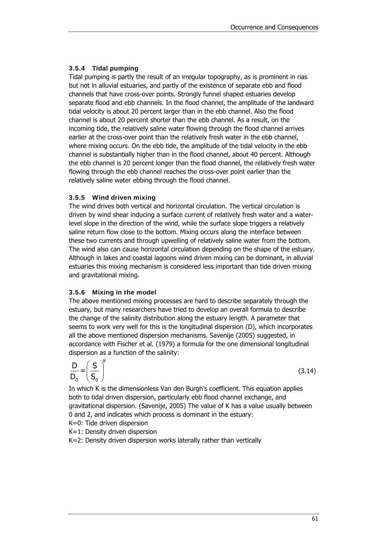
Occurrence and Consequences
61
3.5.4 Tidal pumping Tidal pumping is partly the result of an irregular topography, as is prominent in rias but not in alluvial estuaries, and partly of the existence of separate ebb and flood channels that have cross-over points. Strongly funnel shaped estuaries develop separate flood and ebb channels. In the flood channel, the amplitude of the landward tidal velocity is about 20 percent larger than in the ebb channel. Also the flood channel is about 20 percent shorter than the ebb channel. As a result, on the incoming tide, the relatively saline water flowing through the flood channel arrives earlier at the cross-over point than the relatively fresh water in the ebb channel, where mixing occurs. On the ebb tide, the amplitude of the tidal velocity in the ebb channel is substantially higher than in the flood channel, about 40 percent. Although the ebb channel is 20 percent longer than the flood channel, the relatively fresh water flowing through the ebb channel reaches the cross-over point earlier than the relatively saline water ebbing through the flood channel. 3.5.5 Wind driven mixing The wind drives both vertical and horizontal circulation. The vertical circulation is driven by wind shear inducing a surface current of relatively fresh water and a water-level slope in the direction of the wind, while the surface slope triggers a relatively saline return flow close to the bottom. Mixing occurs along the interface between these two currents and through upwelling of relatively saline water from the bottom. The wind also can cause horizontal circulation depending on the shape of the estuary. Although in lakes and coastal lagoons wind driven mixing can be dominant, in alluvial estuaries this mixing mechanism is considered less important than tide driven mixing and gravitational mixing. 3.5.6 Mixing in the model The above mentioned mixing processes are hard to describe separately through the estuary, but many researchers have tried to develop an overall formula to describe the change of the salinity distribution along the estuary length. A parameter that seems to work very well for this is the longitudinal dispersion (D), which incorporates all the above mentioned dispersion mechanisms. Savenije (2005) suggested, in accordance with Fischer et al. (1979) a formula for the one dimensional longitudinal dispersion as a function of the salinity:
K
0 0
D S=
D S⎛ ⎞⎜ ⎟⎝ ⎠
(3.14)
In which K is the dimensionless Van den Burgh’s coefficient. This equation applies both to tidal driven dispersion, particularly ebb flood channel exchange, and gravitational dispersion. (Savenije, 2005) The value of K has a value usually between 0 and 2, and indicates which process is dominant in the estuary: K=0: Tide driven dispersion K=1: Density driven dispersion K=2: Density driven dispersion works laterally rather than vertically

Salinity in the Casamance Estuary
62
3.5.7 Occurrence of mixing processes in the Casamance estuary In the model a value for the Van den Burgh’s coefficient of 0.75 is used. This value has given accurate results and thus can be concluded that vertical density driven mixing is the most important mechanism in the Casamance estuary. From the salinity distribution curve itself can be determined which mechanism is dominant. A small density gradient indicates that tide driven mixing is dominant, while a strong salinity gradient is typical for gravitational circulation. In figure 15 the salinity distribution curves of the Casamance are shown. It is seen that at the mouth the gradient of the curve is small, thus indicating tide drive. At some distance from the mouth the curve increases rapidly to a peak, after which it rapidly decreases. This curvature suggests that gravitational mixing is dominant. As this is the main part of the salinity distribution, it should be concluded that overall gravitational mixing is dominant in the Casamance estuary.

Occurrence and Consequences
63
3.6 The Salt Intrusion Model
A model is a simplified description of the reality that has the capability to predict the behaviour of nature in certain circumstances. This is obtained through simulating the processes occurring in this system. The original Non Stationary Salinity Intrusion Model Version 5.0 was set up by Savenije (1986 – 1990). This model simplifies the estuary and its processes. The model has been adapted to the Casamance estuary with better and more recent information. A general description of the model processes will be given in paragraph 3.6.1. To assure that the model is a good description of reality, it has to be calibrated and validated. However, a model is a description, which has its shortcomings, therefore in this paragraph also the limitations and sensitivity of the model is described. There are three types of output generated by the model: The salinity at each point in the estuary, the discharge and mixing at each point in the estuary and the bathymetry. The calibration of the bathymetry is already described in paragraph 3.2. The calibration and validation on salinity and discharge will be described in paragraph 3.6.2. The results, sensitivity and limitations will be described in paragraph 3.6.3. 3.6.1 Model processes The salt distribution in an estuary can be described with the unsteady state one-dimensional salt balance equation:
2f
s 20
Qs s rb s D s s rr (1-K) -(1-K) + -D s =0
t A x x a x x hh∂ ∂ ∂ ∂ ∂
+ +∂ ∂ ∂ ∂ ∂
(3.15)
This equation is derived with the mass balance principle. As rainfall and evaporation play an important role in the Casamance, these factors are added in the salt balance equation through the parameter r, which is the effective rainfall e.g. rainfall minus evaporation. The equation is solved with a six-point finite difference scheme. (Savenije, 2005) The model works with a time discretization and a spatial discretization to solve the salt balance equation. The estuary is schematized to a single river and divided in several boxes with length xΔ . The salt concentration within each box is influenced by the flow of water through the box, introducing dispersion, and by rainfall and evaporation. See figure 36.

Salinity in the Casamance Estuary
64
Figure 36: The schematised estuary. The dispersion in every box, Di, is calculated every time step with:
ii i-1 sea
i
QD =D -K x if Q >0
AΔ (3.16)
s,i 2 n,ii sea
2
D +K DD = if Q <0
1+K (3.17)
( )sea f tot e pQ =Q -O R E-R P (3.18)
( )i i+1 box e pQ =Q -O R E-R P (3.19)
is,i s,i-1
i
QD =D -K x
AΔ (3.20)
K
in,i 0
0
sD =D
s⎛ ⎞⎜ ⎟⎝ ⎠
(3.21)

Occurrence and Consequences
65
Ds reflects the dispersion for the steady state and Dn for the unsteady state. The steady state equation is derived on the assumption that the dispersive and advective salt transports are equally strong. Then a tidal average state of equilibrium occurs. The unsteady state dispersion is a better representation of the salt dispersion in estuaries where the equilibrium state is slowly achieved. In that case the system lags behind the steady state situation. The use of the steady state equation leads to a simulation where the dispersion coefficient used corresponds with the ultimate state of equilibrium that would occur if the discharge were maintained constant over a sufficiently long period. The above equations state that if the fresh water discharge into the sea is a positive figure, the steady state equation is used. However, if Qsea is negative, a combination of the steady state and unsteady state is used. The parameter K2 determines the importance of each equation with respect to the other. The initial condition, the salt concentration at t=0, is determined with:
1/K
f0
0 0
KaQ xs=s 1- exp -1
D A a⎛ ⎞⎛ ⎞⎛ ⎞⎜ ⎟⎜ ⎟⎜ ⎟
⎝ ⎠⎝ ⎠⎝ ⎠and
0.141.5f
0 0
Q TD =9 g H
P⎛ ⎞⎜ ⎟⎝ ⎠
(3.22)
With the dispersion distribution known along the estuary, the salt concentration distribution can be calculated for the next time-step. This is done by solving the salt balance equation with the six-point finite difference scheme. 3.6.2 Calibration and validation Calibration is only possible by comparing the modelled output with the values that actually occurred. Since the main goal of the model is to predict the salt intrusion, calibration on salinity is a logical choice. There aren’t many reliable measurements of salinity of the Casamance. Measurements are only useful for calibration if they show the salinity distribution over a long part of the estuary at one moment. These kinds of measurements have only been made from June 1987 until July 1992. This period isn’t long, but quite representative because it contains wet and dry years. The data set consists of salinity measurements that are made each month, on 15 places in the estuary, varying from 63 up to 254 km from the estuary mouth. From these measurements, two important calibration and validation concepts can be obtained: The salinity distribution over the length of the estuary at a certain time, for instance May 1989, and the salinity change over time at a certain place, for instance at 192 km from the estuary mouth. Because the lack of long term data, here is chosen to calibrate visually on one of the plotting methods, and validate on the other one. After this, the other plotting method is used for calibration. The model is calibrated on the plots of May, July and September, since the changes and range are the largest in these months. To adjust the model to reality, there are some parameters that can be changed, and some that cannot be changed in order to keep the model realistic. Parameters like rainfall, evaporation or tidal propagation are parameters that are given facts that can not be changed. Parameters that can be changed, the calibration parameters, are the following: the K2 mixing parameter, which defines the relative proportion of mixing concepts, the ratio rain and the ratio evaporation, which define the ratio relative to the open water surface of the surface that immediately catches rain or immediately

Salinity in the Casamance Estuary
66
loses water by evaporation. These are all parameters that can hardly be measured accurately, only defined by trial and error. The ratio rain and the ratio evaporation have a lot of influence on the speed of response of the model on a change in rain or evaporation.
The ratio rain
Rain that falls on the open water of the estuary immediately contributes to desalinisation, however, rain that falls on for instance the mudflats and mangrove also immediately contributes to desalination. To take this surface into account, the ratio rain is used. It’s a multiplier of the original open water surface. The ratio rain in the model especially has effect on the difference (range) in salinity in the wet and dry season. The ratio rain after some calibration is defined as 3.5. Given the amount of surface with mangrove and mudflats, this is a realistic value.
The ratio evaporation
Like the ratio rain, this is a multiplier of the open water surface area, but now this area that immediately subtracts water from the channel by evaporation. In the model, the ratio evaporation especially influences the salinity peaks. The ratio evaporation has been defined on 1.7.
The K2 mixing parameter
The K2 mixing parameter is calibrated to a value of 0.54. At this value the model performs reasonable both up- and downstream in the estuary, both mixing concepts giving about an equal contribution.
Stability
Another calibration parameter is the calculation place step and the calculation time step. In reality, the choice of these steps should not influence the outcome, but since this model is partly numerical and therefore sensitive for numerical diffusion, the choice of the time and place calculation step has to be taken with care. The risk of numerical diffusion is the least with a small Courant number:
tv
xΔ
σ =Δ
(3.23)
In other words, a combination of a large place step with a small time step. A very stable model however, cannot cope with rapid changes in the salinity distribution. Therefore, finally is chosen for a large place step (5000m) in combination with a small time step (2 days). With these calculation steps the model is stable in almost all cases, and still quite capable to show rapid salinity changes. When a time step of one day is chosen, the model is very stable, but not able to show enough variation.
Validation on discharge
The discharge used in the model as input is the discharge at Kolda. The discharge at the mouth can be roughly estimated by extrapolation of the catchment at Kolda and the catchment at the mouth. This can be compared with the computed values of the discharge in the model which have the right order of magnitude.

Occurrence and Consequences
67
3.6.3 Final results, sensitivity and limitations After many rounds of calibration and validation, the best performing model is found. In the Casamance, the salinity can change very rapidly, and many processes that influence the distribution are not modelled. There are large differences in the dominance of mixing processes upstream and downstream, but this all has to fit in one model. It is possible to define a model that performs well on the upstream part of the estuary and one on the downstream part like it is also possible to define a model that performs well on peaks and one on low values. Making more models for one estuary is however doubtful and the improvement isn’t that large. Therefore finally one model is made. The value of the model is defining the occurring range of salinities, not to define the exact salinity prediction on a certain place and time. Below the model results are given for the salinity distribution in 1989 over the length of the estuary and the salinity distribution at 192 km from the estuary mouth for the measurement period 1989 – 1992.
Salinity distribution 1989
0
20
40
60
80
100
120
140
160
0 20 40 60 80 100 120 140 160 180 200 220 240 260 280distance from estuary mouth (km)
salin
ity (
kg/m
3)
measured may 89measured july 89measured sept 89computed may 89computed july 89computed sept 89
Figure 37: Salinity distribution 1989.

Salinity in the Casamance Estuary
68
model results at 192 km from estuary mouth
0
20
40
60
80
100
120
140
160
29-3-1986
11-8-1987
23-12-1988
7-5-1990 19-9-1991
31-1-1993
15-6-1994
time (dd-mm-yyyy)
salin
ity
(kg/
m3)
192computed
Figure 38: Model results at 192 kilometres from the estuary mouth.

Occurrence and Consequences
69
3.7 Scenarios
The model can be used as a predictive model by checking its response on possible future climate changes. In this paragraph, three scenarios are presented for possible future changes in rainfall and runoff, and their consequences for the estuary are determined. The scenarios that will be discussed are the flushing scenario, which is based on an increase of rainfall, the little rainfall scenario, based on a decrease, and the spreading scenario, which discusses the trend that the same amount of rain falls, but more distributed over the year. 3.7.1 Flushing scenario As was described in chapter 2, the Casamance estuary has become hypersaline during the Sahelian drought. The flushing scenario is set up to check whether this process is reversible, and what must happen to refresh the estuary or, in other words, to flush it. The most important parameter that influences the flushing of the estuary is the rainfall, since this is a dominant parameter with a large variance. More rainfall will result in more runoff. The scenario must answer if efficient flushing the estuary is a process of several years with a lot of rainfall or just one very extreme year. To implement realistic years with heavy rainfall in the model, the three years with most rainfall from the modelled period have been averaged to create a realistic extreme rainfall year (these are the years 1975, 1999 and 2002). Because of the correlation of rainfall and runoff, the same has been done with the runoff of these years. These data have been added after the years 1970 – 2004, and in this way creating imaginary heavy rainfall years, from 2005 until 2010. From the model output can be concluded that the estuary reacts quick on a change in rain and runoff intensity, a new equilibrium is soon reached, in sense that in the second year the salt distribution is the same as in the third year. Another important conclusion is that several years of heavy rain is not enough to flush the estuary completely, which results in a hypersaline estuary in the dry season, however the estuary is reasonably fresh in the upstream part at the end of the raining season, see figure 39.

Salinity in the Casamance Estuary
70
flushing scenario, '2007'
0
10
20
30
40
50
60
70
80
90
100
110
120
130
0 20 40 60 80 100 120 140 160 180 200 220 240
kilometres from mouth (km)
salin
ity
(kg/
m3)
computed may 07
computed july 07
computed sept 07
Figure 39: Flushing scenario ‘2007’. Since long term flushing does not have effect, the response of the model on a very extreme rainfall year is tested. There can be concluded that a rainfall intensity of about twice as much as a ‘normal extreme’ is needed to flush the estuary as a whole. The conclusion that can be made from the model is that hypersalinity in this estuary is more or less irreversible. This is mainly caused by the simple fact that more than half the length of the estuary is mixed from the seaside (200 kilometres), resulting in a salinity of the ocean. During the dry season, which is a relative long period compared to the rainy season, this salinity is transported upstream by the resulting flow due to excessive evaporation. As a consequence of this evaporation, the salinity increases, resulting in again hypersalinity. To flush this part of the estuary that is mixed by the tide and has an ocean salinity, can only be done by pure advection, or in other words, literally refresh all water in the basin.
Marginal comments
The model does not behave very well on peaks, sometimes salinity peaks are quite overestimated, which happens mostly during rainy years like for instance 1988-1989 in the calibration period. This may cause an overestimation of the needed rain to flush the estuary. The order of this estimation is expected to be not so large that the conclusion of this scenario is incorrect. Another comment that can be made is that

Occurrence and Consequences
71
during some years of heavy rainfall, the discharge during the dry season may be underestimated, since this mainly is adapted from single extreme years. 3.7.2 Little rainfall scenario During a longer period of little rainfall an increase in hypersalinity can be expected. On one hand there will be an increase in salinity in the upstream part, and on the other hand the hypersaline zone will grow in downstream direction. The little rainfall scenario is made to determine how far the hypersaline zone can move downstream and in which time scale extreme salinity is reached. For the modelling of the little rainfall the same method is used as the flushing scenario, based on the three years with the least rainfall over the period 1970 – 2004. These are the years 1980, 1983 and 2002. The runoff is also based on these years, however the data of 2002 is discarded because of the influence of a rainy 2001, which is not representative for a period of several dry years. Once the dry years are added to the model, it is noticed that the response of the estuary on dryer years is slower with respect to the flushing scenario; it takes three years before a new equilibrium is reached. As can be seen in figure 40 there is a clear physical boundary in the hypersaline zone extension downstream. Tidal mixing prevents higher gradients to occur. This can be clearly seen from the plot since the gradient increases upstream, where the tidal mixing decreases. The plots show an exponential increase. In figure 40 the year 1992 from the calibration period is added, since this is a dry year as well which shows the same measured results on the gradient.
1992 measured, 2009 dry scenario
0
20
40
60
80
100
120
140
160
180
200
0 20 40 60 80 100 120 140 160 180 200 220 240 260 280
kilometres from mouth (km)
salin
ity
(kg/
m3)
computed april 09computed may 09computed july 09computed sept 09measured may 92measured july 92
Figure 40: Salinity measured in 1992 and modelled in 2009 for a dry scenario.

Salinity in the Casamance Estuary
72
Marginal comments
As mentioned in the flushing scenario, the model overestimates the peaks of wet years. This is not the case for dry years, which can even be underestimated. Comparing modelled results with measured results is a risk here, since peak values are measured on one moment, where the model defines a peak value for the period of ten days, which causes a difference. 3.7.3 Increase in rainfall spreading over time scenario From data analysis with the longest rainfall measurements in the area, Ziguinchor 1918 – 2006, can be determined that the rainfall shows a decrease of 5.8 mm per year on average. A year has 6 months in which it rains significantly, with a peak in July. If the trend per month is analyzed, there can be concluded that with a decrease of 2.9mm per year the peak in August decreases disproportional fast. This causes a flattening in the peak, especially in the direction of September, which decreases only 0.4mm per year. This increase in spreading on rainfall may, besides the decrease in rain, influence the salinity distribution in the estuary. As concluded in the flushing scenario, the estuary responds relatively fast on a higher rain intensity, which hampers hypersalinity. This scenario has been made to check the consequence of a decrease in intensity in the maximum month. For the scenario a year is defined with an average rainfall amount over the year, but with more spreading. For this the average rainfall of the modelled period, 1970 – 2004, is used. The spreading is defined as a decrease of 10% of the rainfall in July, which is spread in relative proportion over the other months. The same is done for the spreading of runoff, with a correction on September, since a lot of rainfall of August comes to runoff in this month. To compare the consequences of spreading, behind the original model first four years with average rainfall and runoff are added, then four years with more distributed rainfall and runoff.

Occurrence and Consequences
73
average, '2008', spreading scenario '2012'
0
10
20
30
40
50
60
70
80
90
100
110
120
0 20 40 60 80 100 120 140 160 180 200 220 240
kilometres from mouth (km)
salin
ity (
kg/m
3)
computed may 08computed july 08computed sept 08computed may 12computed juy 12computed sept 12
Figure 41: Average, ‘2008’, spreading scenario ‘2012’
Marginal comments
However the total rainfall stays the same in each year, the model supports the hypothesis that more spreading results in a more saline estuary. The largest differences occur at the end of the dry season, in May. The differences are however not significant large compared with the quality of the model, to draw accurate conclusions from the scenario.

Salinity in the Casamance Estuary
74

Occurrence and Consequences
75
4 Integrated water management
While this projects focus is on salt intrusion in the estuary, the relation with water resource management in the catchment is important, for it places the research in a wider perspective and might help to investigate the influence of human interference on the salt intrusion. As stated, increase or decrease of salinity levels is largely dependent on the fresh water available for flushing, thus determining a salt accumulation in the estuary in dry years and a general desalinisation in wet years. This is a process on a time scale of years, while salt concentration at a particular location may vary over the seasons in a year. When the yearly evaporation rate is considered rather constant, the rainfall that becomes fast runoff in the estuary is the sole parameter that determines the build up of salt in the estuary. The contribution of subsurface drainage in the later dry season is negligible compared to the open water evaporation as is shown by figure 31 in paragraph 3.4 about the hydrological parameters. The precipitation pattern may vary spatially and in time, e.g. some years have more rainfall in August, while others have more in September and, as discussed in paragraph 3.4, variation in measured rainfall at the different measurement stations is hardly correlated. However, where the evaporation and rainfall are naturally determined by meteorological processes, the quantity of fresh water that becomes direct runoff can be altered by human interference. A dam, for instance, could be used for water retention, thus reducing the fast runoff. This chapter will provide an evaluation of the relevant processes in water resources management in the Casamance basin. First land use and related water management are categorized in three different groups with a typical geographical location, as will be discussed in paragraph 4.1 Water resources and boundary conditions will be discussed per category. After this, the human interference in the runoff process will be discussed in two different subjects; sedimentation and erosion which are closely related and anti salt dams. The first is merely used as an indication for the current state of the water management; the latter is the interface where fresh water discharge, and thus flushing, is most clearly influenced by human interference. This will be followed by a short evaluation of the land side processes that determine the estuary salinity.

Salinity in the Casamance Estuary
76
4.1 Water resources management in the Casamance basin
All processes, problems and interests involved when discussing water related issues on a catchment scale form a complex system. This paragraph’s aim is getting a better insight in the relevant risk, problems and causal relations, by presenting a structured overview in a diagram (figure 42). This will help when making an inventory of further research that is needed or (for the research presented in this report) the relevant human influence on salt intrusion in the basin. It is not possible to fit everything in one scheme and it contains some generalisations, but at least the most relevant risks and problems are drawn. They are subdivided in three groups; drinking water security, low land cultivation and estuary ecosystem, as most problems only occur in one of these categories. One may concentrate on one of these, but it is clear one has to keep the complete picture in mind. Processes and problems are geographically bound and can thus be categorized by a simple subdivision of the terrain. The upstream lowlands, downstream lowlands and higher grounds are discussed here. The last two are the presented in the diagram, but the analysis goes for much of the upstream lowlands as well. Each category is described and analysed below.

Occurrence and Consequences
77
Figure 42: Water related issues in the lower Casamance basin.

Salinity in the Casamance Estuary
78
4.1.1 Higher grounds
Description
These lands can be found throughout the basin, at relatively big distance from the main courses. This is the land where groundnuts are grown, as well as crops like maize. Rain fed rice paddies will occupy the valleys, where the small tributaries or bolons may originate from. The natural vegetation consists of dense (rain) forest. The higher grounds thus are the hill tops and their slopes, which are generally moderate. Cities and villages are often located on the tops, while agriculture is practised further downhill. The forests are well able to retain enough water to survive the droughts, while preventing extensive erosion of the sandy soils.
Problems and risks
Woodland has been cleared for agriculture and (fire) wood and is soon occupied by small villages. The cleared land is less capable of retaining water, although farmers put much effort in protective measures in order to minimise crop damage by erosion, drought and land degradation due to wash out. A decreased retention usually means less infiltration and thus a lowering of the phreatic groundwater table, which is re-enforced by the reduction of deep rooting plants. This could explain lower water levels in the wells in the dry season and pose a risk when fresh water pressure and flow further downhill is reduced, giving salt estuary water the chance to infiltrate further landwards. The latter is an extra storage of salt in the estuary, as well as a problem when salt water reaches the drinking water well. The specialist from the GDR states that this risk is only existent in the coastal area and islands, where the salt water intrudes from different directions and permeability is high i.e. sands without natural protective clay layer. The presented figure displays these risks and problems: the increased fast runoff and reduced infiltration result in a lower groundwater table (resulting in drought) and the risk of further salt intrusion. The risk of contamination of the drinking water that is extracted from the subsoil is biggest in urbanised area and can be caused by industry and construction as well as for example leaking sewerage and latrines, as is the case in Ziguinchor (Personal communication, Badiane, GDR) . Costs and dangers related to extensive erosion are omnipresent in the basin, as will be discussed in next paragraph. As erosion is most severely felt in areas with (moderate) slopes and urbanisation, the higher grounds can be considered to have the highest erosion risk.
Remarks
A critical note might be that a lowered groundwater table can be caused by little rainfall as well as lack of infiltration. Water retention in the rainy season however, is the only way to prevent dramatic drought and its consequences in the dry season. When retention and infiltration is reduced, by for instance clearing land and leaving the ground fallow (more fast runoff), the drought will be more severely felt.

Occurrence and Consequences
79
4.1.2 Downstream lowlands
Description
This area is characterized by the tidal floodplains that get flooded year round. This is 'mangrove country', which is naturally ‘inundated’ with seawater by numerous small meandering creeks. Fishery and oyster collection, important protein rich food resources, thrive here very well. The ecosystem is very rich and diverse (Niang-Diop, 2002) and salinity levels never reach dramatic levels. This part of the estuary is well mixed by seawater that enters with the tide, which prevents the water from becoming very saline. Tidal currents are strong enough to carry nutrients to the mangroves. When this process fails the mangroves extinct, leaving the bare mudflats or 'tannes' behind (Marius, 1982). For ages the local inhabitants have reclaimed the fertile but salty grounds along the river by building dikes in order to prevent salt intrusion from the river. Generally a band of mangroves is left to protect the dikes from scouring and erosion. The first rows of dikes are used to retain fresh water as buffer for the salt intrusion. Nowadays these basins are often used to bring up small fish that is caught in the river, or even breeding young fish, in the case of the Kagnout polder system. Further inland the ground is suitable for growing rice (see below).
Figure 43: Picture of a part of Kagnouts polder system, provided by Google EarthTM

Salinity in the Casamance Estuary
80
The main course of the estuary is located in north-western direction. The small creeks that distribute water to the mangrove flats and eventually the polder system are clearly visible. The band of mangroves that protects the polder system is comparatively large, but will become smaller when more land is reclaimed. When zooming in one clearly recognises the larger paddies on the west side that are used as fish basins and salt intrusion prevention. The little white and light green fields are all used for growing rice.
Figure 44: Polder system at Kagnout in more detail. The villages itself are further uphill and might be described as a higher ground. With all the generalisations involved it is difficult to determine are fixed boundary between these categories, as one refers to Kagnout for its polder system, while the village itself is located just outside. It seems best to define the villages as the interface where both types of land meet, as further inland the tidal influence will not be present. The upstream boundary along the main streams between the upstream lowlands and the downstream lowlands is hard to define. It must lie upstream of Ziguinchor, where salinity level is about as high as at sea and tidal influence is strong as the upstream lowlands are defined as the flats that are most severely afflicted by hypersaline conditions. One might take the habitat of the Rhizophora mangrove as the boundary, as the die out of this species is often directly related to dramatic hypersalinity.

Occurrence and Consequences
81
Problems and risks
As stated, hypersalinity is not really a problem in the downstream lowlands as society and vegetation are used to the rather constant salinity levels that do not fluctuate much over the seasons and years. The affected area with dramatic hypersalinity will increase as more salt is accumulated in the estuary. When looking at the polder systems, there are two governing boundary conditions; the saline estuary water that intrudes in the dry season, as the fish basins are not capable of preventing intrusion, and has to be washed out with the first rains. Secondly, the potential acidification by oxidation of the pyrite that is present in the soil. Ground that has had mangroves on it is often very pyrite rich. Oxidation occurs when the land is over drained, of soils are excavated, inducing a rapid and severe acidification of the soil, where upon no consumptive plants can grow. Agricultural yield can be sufficient for the local population, but requires good (water) management and maintenance of the polder system. Societal changes like a strong migration of people from rural land to bigger cities might hamper the manpower in the village necessary for maintenance. Non governmental organisations as for instance IDEE Casamance recognise the risks related to insufficient management and start up programs for better education and improvements in construction and maintenance techniques. In the case of the Kagnout polders, this has led to a better fish production and much abandoned land being recovered and new land reclaimed, showing that much problems can be omitted. Sometimes anti salt dams are built in order to prevent salt intrusion from the estuary and reclaim big valleys for rice production. These projects are generally of a much larger scale than the polder systems and thus require more sophisticated management to prevent acidification problems as many unsuccessful projects show (Guidel and Affiniam dams). A more in-depth analysis of the issues involved is presented in paragraph 4.3. As discussed above, saline groundwater can be a problem when it contaminates drinking water. While the problems can be very local, the processes involved may be of a larger scale; the long time water resides in the ground and the big distance it travels, before it is actually extracted. Deposition of eroded sand might cause problems in the lowland rice paddies, as it can cover the plants and make the soil less fertile. Damage to dikes and crops when the paddies get flooded with much water from urbanised area is related to this. Erosion and sedimentation will be more thoroughly examined in paragraph 4.2.
Remarks
The estuary itself can be seen as a part of the lowland area as well. Degradation of its ecosystem is most heavily felt in the upstream parts, where the conditions for flora and fauna are most extreme (extreme variance in salinity) and eutrophic monocultures will be found (Niang-Diop, 2002). As the lowland area does not suffer from these extreme conditions, it might seem that the problems in the downstream part are minor. However, the impact of increased urbanisation is great; over fishing, logging of mangrove and pollution from human developments.

Salinity in the Casamance Estuary
82
4.1.3 Upstream lowlands
Description
Upstream lowlands, a rather contradictive term at first sight, must define the flat lands, usually located along the banks of major streams of the estuary, where the tidal influence is not very strong. These lands are found further east and northwards where the salinity levels are high. Natural vegetation has been reduced by the ‘recent’ salinisation of the estuary leaving bare mudflats behind, where mangroves grew before. Due to the high salinity levels and lack of ‘refreshing’ flows, Rhizophora mangroves don’t survive here and fish, mainly Tilapia, do not grow big. Rainfed rice production is possible as long as salt intrusion can be prevented by dams or dikes or flushed with the first rains of the season. In the dry season many tidal flats fall dry when the mean water level is lowered by the annual fluctuations described in paragraphs 2.3.
Problems and risks
Hypersalinity is the main problem in this area. Agriculture and fishery suffer much from high salinities and the ecosystem is far from diverse. Fresh water is more scarce here, since rainfall is often less than in the downstream lowlands, thus making the condition for agriculture less favourable, but not impossible. Potential acidity is a risk here as well, but can be said to be minor compared to the hypersalinity, for acidification can be prevented with good management, as long as sufficient fresh water is available, which is often not the case. Erosion and sedimentation and damming are important issues in the upstream lowlands, but will be dealt with separately as explained before. Most damming projects however have been in the downstream area as the conditions are better and the region more densely populated. Urban erosion thus might be a bigger problem in the downstream lowlands as well.
Remarks
Very high salinity levels do not directly give favourable conditions for salt winning. It is practised here but only on a small scale (by collecting). The reason for this is the small tidal range thus making it impossible to ‘trap’ much salt water. Evaporating of trapped salt water is the general practise of larger scale salt winning, and here thus not very profitable.

Occurrence and Consequences
83
4.1.4 Overview One could summarize the mentioned problems and risks in a table: occurrence higher
grounds downstream lowlands
upstream lowlands
parching X X X contamination X X X erosion X silting up X X salt intrusion subsoil x X X hypersalinity X acidity X x x: relative small risk X: relative big risk
Table 7: Risks in the Casamance estuary. It is clear that the problems related to the estuary salinity are more severe when one is further upstream. As modelled and explained in chapter 3, the estuary is not likely to recover and will remain very hypersaline in the upstream part. This hampers development of the region that is indeed less urbanized than the downstream lowlands, which have a better climate for agriculture and fishery as well. One may conclude from this that more attention to the upstream region should be paid, in order to prevent further inequality between these regions, for example by focusing on productive sustainable salt winning. Human interference could influence estuary salinity, when the flushing component of the rainfall is reduced by retention with dam and terraces. As a spreading of the rainfall and discharge over time does not really affect the salt distribution in the main course, one could say that small scale retention of water for agriculture does not conflict with desalinization of the estuary (complete desalinization appears to be impossible any, since it requires too much fresh water inflow). Larger scale retention by damming of larger valleys and branches will affect the main course of the estuary, as it diminishes the tidal prism and the fresh water inflow very much. Whether this big scale projects have a positive or negative affect on the salinity in the estuary, demands further research. This clearly conflicts with fishery interest, as higher salinity levels will lead to a smaller fish population. The reduction of viable mating grounds and habitats has a big influence as well. As the complexity demands an integrated approach, it is good to state that for example acidification and contamination are problems that are induced rather locally, by bad management or maintenance.

Salinity in the Casamance Estuary
84
4.2 Erosion and sedimentation in urban areas
Besides the erosion and sedimentation problems in the Casamance estuary, great problems with erosion and sedimentation occur in the urbanised areas. Erosion causes many problems with sandy roads and the foundation of houses. Rice paddies which provide the main source of food for the local habitants are filled with sedimentation, making the rice paddies useless. 4.2.1 Area description Let’s first describe the manner how land is reclaimed for human use. People tend to settle near coasts and rivers for fertile grounds. But to protect themselves and their properties from the water, high grounds near the rivers are sought to build their houses. The land is cleared from most of the trees and other vegetation and houses are built. Between the houses usually roads are built or created naturally, constructed only of sandy soils. Ziguinchor is a wide city, which can be seen as a big village consisting of low-rise buildings and many streets. Main roads are mostly constructed with an asphalt layer on a sand layer, see the upper picture, secondary roads consists usually only of sandy soils, as can be seen in the lower picture of figure 45.
Figure 45: Examples of the infrastructure in Ziguinchor; main road (above) and secondary road (below).

Occurrence and Consequences
85
At the borders of the village rice paddies are created for own consumption. Hardly any protection against erosion is done on the houses with its surroundings. The nearby rice fields are mostly fed by direct rainfall. 4.2.2 Erosion Erosion occurs in hilly areas consisting of less cohesive soils and is caused by fast runoff. The transport capacity increases with higher water velocities, which occur with steeper slopes and long intensive rainfall. Vegetation at areas with steep slopes prevents a part of the erosion due to the roots which increase the cohesion of the soil and the infiltration. Erosion is generally seen as a form of land degradation and it's widely accepted that this has to be prevented.
Figure 46: Erosion and sedimentation problems in rural (left) and urban (right) areas. Figure 46 shows that land cultivation can result in erosion. Often rural activities end up in less fertile grounds, and when these grounds are abandoned often erosion occurs on these fallow lands. In urban areas erosion occurs mostly due to a lack of vegetation, and thus less cohesive soil. In the urban areas within the Casamance region, retention and infiltration decreases due to the loss of vegetation. The upper ground consists mostly of sandy soils and erodes extensively. Here several examples of erosion in Ziguinchor are presented.

Salinity in the Casamance Estuary
86
Figure 47: Example of the start of urban erosion. In this picture can be seen that the roads without any solid layers become useless during heavy rainfall.
On a long scale this urban erosion causes more and more problems with the infrastructure. The picture below is taken in a quarter of Ziguinchor and shows a canal with a depth of almost three metres. This make the foundations of the nearby houses very unstable, it is quite dangerous. Houses collapse due to erosion on foundations, sometimes with deadly consequences. On top of that, one can understand that this ‘eroded canals’ are often much polluted.

Occurrence and Consequences
87
Figure 48: Example of extensive erosion in a quarter of Ziguinchor. As mentioned above, the complete infrastructure has to deal with the problem of erosion. Below is a picture of a bridge which is also damaged by the force of the rainwater. It can clearly be seen that this kind of structures cannot cope with the current rainfall. The question is if this is due to a failure in the construction, or due to a lack of complementary measures.
Figure 49: Also the road structures are in danger. Because of the urban erosion, the quality of the roads is reduced very rapidly. After a couple of years, the roads are in the condition such as those in the pictures.

Salinity in the Casamance Estuary
88
4.2.3 Sedimentation A lot of sediment comes from urban areas uphill and flows directly to the lower situated rice fields, see figure 50. Many rice fields are situated in the city itself. The small dikes around the fields are damaged by the huge floods and cannot protect the paddies against the floods. After entering the rice paddies the surface runoff water deposits the sand. Therefore a lot of rice paddies will silt up with sand and become useless.
Figure 50: Rice paddies in Ziguinchor. On the left: recently silted rice fields. On the right: water flowing through an area which consisted of rice paddies several years ago. Besides the problems with sedimentation in the rice fields, some drainage channels which are constructed became useless because of huge sedimentation problems. Also a lot of garbage is stored in the drainage channels. Examples of these problems in Ziguinchor can be seen in figure 51.
Figure 51: Two examples of sediment and garbage problems filling up the existing drainage canals.

Occurrence and Consequences
89
4.2.4 Solutions The best way to prevent the problems discussed above, is an integrated approach with measures on all the different problem subjects, and thus all the different locations. However, an integrated approach is expensive and is therefore quite unlikely to happen. Prevention of the majority of the erosion problems causes of course much less sedimentation problems. To prevent erosion in this region, several solutions are considered in this paragraph. The best way to prevent erosion in urban areas is to build drainage channels along the road. In several districts, this is already done, only with little results. As discussed above many channels are filled with sediments within a few years. A couple of improvements have to be made to improve the function of the drainage channels. At first the channels in urban areas have to be closed at the top side, so that only little sand can enter the channel via this way. Otherwise much sand or garbage will enter the channel due to wind, runoff or human interference. The best way for runoff to enter the channel is by horizontal gates. In this way not all the sand and garbage comes to runoff with the rain. Horizontal gates will also prevent big pieces of garbage of entering the channel. A road with good foundation, sidewalks and drainage channels will be a good way to prevent urban erosion. Another way to prevent the outflow of sand around the houses is to construct walls around the gardens. In this way the sand will not be able to flow out of the gardens. However, this solution will be difficult to implement because of the relations between families and their houses. Most families would not like to build a construction wall around their territory, although it might be a small wall. A third solution for the urban erosion problem is to plant trees or plants along the road. This will cause less erosion along the road, although the complete problem isn’t solved. Trees which can be useful are fruit trees, for the local inhabitants will have extra advantages by means of the fruit. Otherwise maybe the trees are used for firewood. Good agreements have to be made between the municipality and the local residents about maintenance of the trees. The last solution to prevent urban erosion is to collect rain water that falls on houses, i.e. by means of water butts. In this way less water will flow on the surface, and thereby causing less erosion. The four suggested solutions together with the solutions on other sectors are listed in table 8.

Salinity in the Casamance Estuary
90
urban rural
- construction of drainage channels - no fallow lands - retention of rain water - better land management - vegetation - organization of farmers
erosion
- building of fences - cleaning of drainage channels - covering of drainage channels - irrigation system with sand trap - building of pavements - division of rain
sedimentation
- division of rain water
Table 8: Solutions for urban and rural erosion and sedimentation on a small scale. Besides the measures on erosion, sedimentation can be prevented by certain measures. However, problems with sedimentation will only occur secondly, while erosion is the primary problem. An important measure is the cleaning of drainage channels. In the current situation this is hardly done, so that the drainage channels cannot fulfil their function. Covering the channels is another way to prevent sedimentation, as stated above. On top of that, division of rain water will give more control on the ways of the rain water. A great part of the rural erosion can be prevented by better land management and organisation of farmers. Accumulation of fallow lands will definitely cause erosion when the rainy season comes. However, to prevent this, the local farmers have to communicate with each other. An organisation of farmers can be formed, for their own interests. The local authorities will play an important role in the first steps of this organisation. Once erosion occurs, sedimentation will occur nearby. A big problem will be the sediment in the drainage channels. Although little sediment will enter the channel when horizontal gates are constructed, after several years this sediment will silt the channel. Therefore at least once a year this sediment had to be cleaned, probably by the municipality service. A complete different kind of approach is to prevent the sediment from entering the rice fields. This is difficult to effectuate. A solution will be the construction of an irrigation system to control the water that enters the paddies. In this way division channels have to be build to lead the water into the rice paddies. To prevent the sediment from entering the paddies, a sand trap has to be constructed in front of the inlet. This trap has to be cleaned from time to time to function properly.

Occurrence and Consequences
91
4.3 Anti salt dams
Several anti salt dams have been constructed in the catchment of Casamance estuary. The dams are built in tributaries of the Casamance estuary to reclaim salty upstream grounds and use the land for rice cultivation. The anti salt dams can have a considerable impact on the environment, both positive, as well as negative. The sudden local change from salt into fresh water and a change of water velocity create a different habitat. These changes have their effects on the sedimentation, flora and fauna. There are several types of anti salt dams in the Casamance catchment. The ones that are taken into account here are the dams which are placed in secondary or tertiary channels. The Casamance estuary is considered here as the primary channel. Bolons like the Soungrougou at Adéane and the Diouloulou just downstream of Pointe St. Georges, mentioned in chapter 2, are examples of secondary channels. Tributaries that end up in a secondary channel are called tertiary channels. The dams that are placed in the secondary and tertiary channels prevent salt to intrude into the estuary branches. The creation of anti salt dams will cause a change from a salt environment into a salt environment on the upstream part of the dam. This change can have an effect on fairly large sub catchments and is considered to have potentially big influence on the environment. The anti salt dams can have weirs or gates, which make it possible to manage the water levels on the upstream part of the barrage. From the dams named below some just consist of a dam with an opening. Water is able to flow here in and out. With this type of construction salt water is still able to reach into the branches. Many smaller dams, or dykes, which have been constructed in the area, are built to prevent intrusion of salt water from the estuary into rice fields. These dams protect small pieces of land and are considered to have far less influence on the environment, compared with the larger dams which have influence on a whole sub catchment. Most of these dykes don’t have gates or weirs and so it is impossible to regulate a water level in the polder system. Other dykes do have gates or weirs and so these have their effects on the water level in the polder. But the influences of these barrages are nonetheless considered to be very small compared with the large dams. Since 1983 several anti salt dams have been built in the downstream part of the Casamance estuary. Nine dams are located at the north bank of the estuary, near the villages of Affiniam, Babat, Bona, Diatang, Djinaki, Djinoubor, Kolomba, Santak and Silinkine. On the south side of the estuary there are dams near Niaguis, le barrage de Guidel and near Simbandi. The exact locations are given in figure 52.
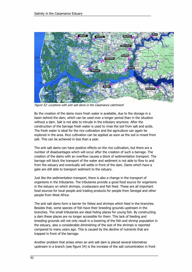
Salinity in the Casamance Estuary
92
Figure 52: Locations with anti salt dams in the Casamance catchment By the creation of the dams more fresh water is available, due to the storage in a basin behind the dam, which can be used over a longer period than in the situation without a dam. Salt is not able to intrude in the tributary anymore. After the construction of the barrage fresh water is used to rinse the soil from salt and acids. The fresh water is ideal for the rice cultivation and the agriculture can again be explored in the area. Rice cultivation can be applied as soon as the soil is rinsed from salt. This can be achieved in less than a year. The anti salt dams can have positive effects on the rice cultivation, but there are a number of disadvantages which will occur after the creation of such a barrage. The creation of the dams with an overflow causes a block of sedimentation transport. The barrage will block the transport of the water and sediment is not able to flow to and from the estuary and eventually will settle in front of the dam. Dams which have a gate are still able to transport sediment to the estuary. Just like the sedimentation transport, there is also a change in the transport of organisms in the tributaries. The tributaries provide a good food source for organisms in the estuary on which shrimps, crustaceans and fish feed. These are all important food sources for local people and trading products for people from Senegal and other people from West Africa. The anti salt dams form a barrier for fishes and shrimps which feed in the branches. Besides that, some species of fish have their breeding grounds upstream in the branches. The small tributaries are ideal hiding places for young fish. By constructing a dam these places are no longer accessible for them. This lack of feeding and breeding grounds will not only result in a lowering of the fish and shrimp population in the estuary, also a considerable diminishing of the size of the shrimps is reported compared to many years ago. This is caused by the decline of nutrients that are trapped in front of the barrage. Another problem that arises when an anti salt dam is placed several kilometres upstream in a branch (see figure 54) is the increase of the salt concentration in front

Occurrence and Consequences
93
of the dam, the part of the tributary which is still in contact with the estuary. By placing the dam some kilometres upstream of the tributary the tidal prism of the tributary becomes much smaller, because the surface area upstream of the dam is no longer included in the tidal prism. This will result in lower velocities with the consequence that salt can not be flushed out of the stream. The water remains in for a long period at the end of the tributary and is very sensitive to evaporation and the salt concentration goes up. Land can become useless after an anti salt dam has been constructed. This happened near Affiniam, see figure 53. The land that was planned to be used as rice fields started to become acid due to died mangroves, from which the roots oxidises after the land is laid dry. The mangroves die when there is no tidal movement anymore.
Figure 53: Anti salt dam at Affiniam. As can be seen in figure 54 and 55 there are different positions to place an anti salt dam in a tributary. In situation A the dam is placed some kilometres upstream from the main stream in the tributary. In situation B the dam is positioned at the mouth of the tributary. Advantages and disadvantages of the two situations are listed in table 9.

Salinity in the Casamance Estuary
94
Figure 54: Anti salt dam placed in the middle of a branch.

Occurrence and Consequences
95
Figure 55: Anti salt dam placed at the end of a branch.

Salinity in the Casamance Estuary
96
Figure 54 Figure 55 Smaller area can be reclaimed for agriculture Larger area can be reclaimed for
agriculture A lot of sedimentation on the estuary side of the dam, which will happen in a few years time
Little sedimentation on the estuary side of the dam
Salt concentration will increase in between the estuary and the dam, compared with the estuary, which will happen in a few years time
No differences in salt concentration at the mouth of the tributary and the estuary
On short term fewer mangroves die Many mangroves die within months Fishery is still possible in the part of the tributary which is in contact with the estuary
Fishery is not possible anymore in the tributary that has been cut off the estuary
A smaller area is exposed to danger of acid sulphates
A larger area is exposed to the danger of acid sulphate
Table 9: Advantages and disadvantages on two different positions of an anti salt dam in a tributary.

Occurrence and Consequences
97
5 Conclusions
The Casamance estuary turned hypersaline in the late seventies due to less rainfall. These high concentrations of salt have a big influence on the flora and fauna, whereby most plants die and leave empty tidal mud flats. The decrease of rainfall lasted until the mid nineties, when a slight recovery of the rainfall is seen. However, the amount of rainfall is not yet at the level of the sixties. The hypersalinity of the Casamance estuary has been studied with a salt intrusion model. It is seen that for consecutive years of equal rainfall the salt distribution shows a pattern through the year. At the end of the rainy season, from June till October, the salt concentrations are less high than at the end of the dry season. Also the concentration peaks are found further downstream at the end of rainy season than at the end of the dry season. These effects are caused by the varying fresh water discharge during the rainy season, which refreshes the saline water. The results of running some scenarios with the salt intrusion model are: • To turn the Casamance estuary into a normal estuary again, a year with a rainfall
twice as high as a wet year is needed. • Several wet years are not sufficient to turn the estuary normal again, only a new
equilibrium is reached. • The salt distribution adapts faster to an increase of the fresh water discharge,
than to a decrease. • A more spreaded rainfall over the rainy season makes the estuary more saline. • There is a limit to the highest salt distribution over the estuary, which has an
exponential form in the part that is under influence of tidal mixing. The relation between the estuary and water resources management in the basin has been investigated in order to get a better insight in the relevance of involved processes and place the research in wider context. It helps to find relations between different problems and their cause and locate the risk geographically.
• Hypersalinity is the main problem in the upstream part of the estuary where tidal
influence is small. Related bad prospects for agriculture and fishery limit development of the region. Since the salinity here is not likely to increase, there should be a focus on prevention of contamination of drinking water by salt intrusion and improvement of salt winning techniques.
• Potential acids are an important boundary condition for agriculture in the downstream lowland area. Good management is needed to prevent problems.
• Erosion and sedimentation are a problem urbanized areas. Poorly protected constructions in sloping areas are very susceptible to extensive erosion. Eroded sediment might silt up rice paddies further downhill. An integrated approach is needed to improve the situation, while prevention of erosion is the best measure to start with. Drainage channel in the city prevent damaging of constructed road and vegetation and fencing can reduces the erosion rate.
• Anti salt dams that have to prevent salt intrusion and are used to reclaim large valleys for agriculture are constructed throughout the estuary. Some with more success than others, due to the acid sulphates present in the subsoil. The land upstream of the dam can be desalinized. The impact on the local environment is big. Many mangroves will die, the sediment and nutrient transport changes and the mating ground for many species becomes inaccessible. The impact on the estuary salinity is hard to determine.

Salinity in the Casamance Estuary
98

Occurrence and Consequences
99
6 Recommendations
The table below summarizes the recommendations for further research that are discussed afterwards. The most important parameters that need more investigations are in bold. Neglected large tributaries, storage width and storage of salt are not implemented yet, while the uncertainties in evaporation and fresh water runoff are relatively large. Variables Information available Further research necessary Shape of estuary Relative old Silting up of the estuary Influence of large tributaries on salt
distribution Better measurements of the present bathymetry Influence of other tributary flowing into ocean Storage width Some Influence of varying storage width on tidal
propagation and salt distribution
Phase lag Some Research on propagation of tidal wave through the estuary
Tidal prism Some Influence of tidal prism on salt distribution Spring-neap variation Water level measurements Influence on intrusion of tide and salt water
storage Inter tidal variation Water level measurements Influence on intrusion of tide and salt water
storage Rainfall Good No Evaporation Measurements with gaps
of one station Better measurements throughout the year and more stations
Fresh water discharge Some Better measurements throughout the year, both more accurate and know cross-section
Mixing processes Not much What processes are dominant at a particular location in the estuary
Calibration of Van den Burgh's coefficient in the salt intrusion model
Salinity Years 1987 until 1992 More accurate data on a higher interval Storage of salt in the estuary during dry
season on tidal flats and in groundwater
Numerical scheme Better approximation on extreme changes in salinities
Intrusion length Some Extend modelled length; further than tidal influence
Tidal damping Good Implementation in salt intrusion model; varying damping term per reach
Side branches Good Implementation in salt intrusion model Storage width Some Implementation in salt intrusion model
Table 10: Summary of recommendations for further research, with the proposed improvements for the salt intrusion model at the bottom.

Salinity in the Casamance Estuary
100
6.1 Data
Rainfall is the most reliable parameter; the rainfall input consists of an analysis of data of the last 35 years. Evaporation is less reliable, because three sources of evaporation types gave complete different data. In the salt intrusion model an important assumption is made, namely an average annual evaporation. Since there is no correlation between rainfall and evaporation on a yearly basis, a modelling of the evaporation by means of temperature, hours of sunshine, wind and humidity on a monthly basis will improve the results of the salt model greatly, for its accuracy is limited by errors in input data. In the input data for fresh water discharge, several data intervals are missing, which makes this input less reliable. However, it would be hard to find these missing data intervals. Better measurement of discharge, from various side branches preferably, would improve the insight in this flux. This is important for water resources management in the catchment as well, for one could have a sound estimate of the available water for agriculture when one would start with measures to increase water retention. This demands a good insight in the rainfall runoff relation. Salinity measurements were not very well available for this research. Best would be to make a monthly set of salt measurements at different locations in the Casamance, to determine the movement of the salt bulge over the seasons. The relation between the salinity and fresh water runoff then might be estimated statistically as well. After about ten years a good calibration of the actual situation can be made. This information is also very useful for research on other topics, such as ecology.
6.2 Model
The modelling of mixing in estuaries is a relative unknown part of research. All different mixing processes are here implemented with one longitudinal dispersion relation, while several mixing processes occur at the same time on different parts of the estuary. Throughout the year the importance of the particular processes changes and thus leads a general dispersion relation to an underestimation and overestimation at some parts of the estuary. A very important shortcoming of the salt model is the numerical diffusion and stability. When stability is guaranteed, the model can not cope with rapid fluctuations in space and time. A better (more stable) numerical solver mechanism will improve the model, and probably simulate the extreme saline peaks better. The water level variation over the year has its influence on the salt distribution that is not taken into account. Additional storage of salt as crusts on the flats that fall dry in the dry season, salt winning and salt intruding in the groundwater aquifers along the stream are not modelled either. The stored salt will be released at the beginning of the wet season, when the soils are rinsed. An accurate salt balance thus can not be made yet.

Occurrence and Consequences
101
Tidal damping is modelled as an average over the whole stream length, which induces a wrong representation of the fluxes involved for mixing. The linearization of the stream width is justified, as the improvements done, doe not really alter the model output. The storage width might fit an exponential shape as well, but is not measured since it cannot be implemented in the model. All land overgrown width mangrove contributes to the inter tidal storage and thus has its influence on the mixing. The tidal prism is generally underestimated. The storage width determines the open water surface susceptible to evaporation and a good estimate of its magnitude and variation over time (the flats that fall dry for example) will improve the accuracy of the model since it becomes more certain that the right processes are modelled and not just calibrated to fit the sparsely available data. During the research, questions arose whether the tidal prism in the main course of the estuary increases or decreases due to the construction of anti salt dams in the side channels. One can say that the tidal prism will increase due to a decrease of friction (the construction of anti salt dams makes the estuary more like a straight channel). One can also say that the tidal prism will decrease due to the diminution of open water surface. The consequences for the salt distribution of a change in tidal prism are also hard to define. This topic needs further research. Finally the fresh water inflow in the estuary will decrease because of the anti salt dams. By these two facts, and the influence on tidal propagation, the influence of the anti salt dams on the salinity in the estuary isn’t clear yet. To clarify these effects, more branches of the estuary have to be taken into account in the salt intrusion model.
6.3 Hydrologic Cycle
For a better understanding of the hydrology of the catchment can improve the water resources management. Characteristics of the subsurface flow, groundwater storage and the rainfall runoff relation are hardly known and are important boundary conditions for water management. Related problems like contaminated groundwater and lowered groundwater tables, as well as fresh water runoff available for agriculture or desalinisation of the estuary demand further research on the water fluxes in the basin.

Salinity in the Casamance Estuary
102
References
Literature
Brunet-Moret, Y., 1970 – Etudes hydrologiques en Casamance. ORSTOM Rapp. Hydrol., 54 pp. Debenay, J. P., 1984. – Distribution ecologique de la microfaune bentique dans un milieu hypersalin: les foraminifères du fleuve Casamance (Sénégal). Doc. Sci. CRODT. Debenay, J. P., 1986. – Première carte bathymetrique entre Adeane et Goudomp. “Etude des estuaries et lagunes du Sénégal: Casamance et Joal – Fadionth” EPEEC / UNESCO Div Sci. Mer / ROSTA, Dakar. Fischer, H.B., List, E.J., Koh R.C.Y., Imberger J., Brooks, N.H., 1979 – Mixing in inland and coastal waters. Academic Press, New York. Garnier, R., 1976. – L’Equateur météorologique, La Météo, VI série, 6, 113-136. Marius, C., 1982. – Acid Sulphate soils of the mangrove area of Senegal and Gambia, Office de la Recherche Scientifique et Technique, Outre-Mer, Paris. McKoy, J.F. Geo-Data; The World Geographical Encyclopedia, Third Edition, 2003. – printed by Gale Group, Farmington Hill, USA. Niang-Diop, I., Dansokho, M., Ibrahima, L.Y., Niang, S., 2002. – Senegal National Report phase 1: integrated problem analyses, GEF MSP Sub-Saharan Africa Project: 2002 Pagès, J., Debenay J.-P., Lebrusq J.-Y., 1987. – L’environnement estuarien de la Casamance, p 191 – 202 Savenije, H.H.G., 1992. – Rapid Assessment Technique for Salt Intrusion in Alluvial Estuaries, International Institute for Infrastructural, Hydraulic and Environmental Engineering, the Netherlands. Savenije, H.H.G., 2005. – Salinity and Tides in Alluvial Estuaries, Elsevier. Savenije, H.H.G., 2006 – CT5450 Hydrlogy of catchments, rivers and delta’s: lecture notes CT5450, TU Delft, Faculty of Civil Engineering and Geosciences. Savenije, H.H.G, van den Akker, C., Boomgaard, M.E., 2006. – Hydrologie 1: college dictaat CT1310, TU Delft, Faculty of Civil Engineering and Geosciences. Stewart R.H., 2006 – Introduction to Physical Oceanography, Department of Oceanography, Texas A & M University, September 2006 Edition.

Occurrence and Consequences
103
Thiam E.H.I., Singh V. P., 1998 – Spatial and temporal variability of salinity in Casamance River Basin, Southern Senegal, West Africa ; Hydrological Processes 12, 1095±1110. Vieillefon, J., 1977. – Les sols des mangroves et des tannes de Basse Casamance (Sénégal) O.R.S.T.O.M., Paris. Ward, R.C., Robinson M., 2000 – Principles of Hydrology: fourth edition, McGraw-Hill Publishing, London;

Salinity in the Casamance Estuary
104
Software
Calculating and modelling
• Non Stationary Salinity Intrusion Model, Version 5.0 may 1990, Euroconsult / IHE by H.H.G. Savenije
• Duflow Modelling Studio • Mathworks Matlab • TotalTideTM, version 1.3.0.2, United Kingdom Hydrographic Office & Cher Salt Ltd. • Microsoft Excel
(Hydrographical) maps
• C-Map World for Windows, Copyright © 1996 C-Map Norway. Hydrographical maps Casamance 1:35,000
• Google Earth
Drawing and designing
• Microsoft Visio • Microsoft PowerPoint • Autodesk AutoCAD
Word processing
• MS Office • Adobe PDF • Euroglot

Occurrence and Consequences
105
Data
Geography and bathymetry
• C-Map World for Windows, Copyright © 1996 C-Map Norway. Hydrographical maps Casamance 1:35,000
• Hydrographical maps Casamance 1:500,000 (French and Portugese Government 1942-1959 additions and corrections to 1960)
• NASA, U.S. Geological Survey, (2002). – Shuttle Radar Topography Mission (SRTM) Elevation Data Set
• Various cross sections and volumes: (Saos J.L., Le Bouteiller C., Diop E.S. (1987). - Aspects Geologique et Geomorphologique de la Casamance, Rev. Hydrobiol. Trop.)
• Storage surface, marsh areas added for different compartments of the Casamance (Brunet – Moret (1970)
Discharge
• Average discharge per year, various stations in the period 1935–1987 • Data Global Runoff Data Centre
Stream velocity
• Stream velocities during various tide cycli at Ziguinchor, at Hamdalaye, near Sefa, 1985
Precipitation
• Genie Rurale, yearly, monthly and daily precipitation, various stations, in the period 1918-2006.
Evaporation
• Evaporation stations of the years 1971 until 1981 at Ziguinchor (1971 – 1981), Sefa and Kolda. Also some temperature and wind data. (Dacosta 1989)
• Potential evapotranspiration in Ziguinchor as calculated by the FAO for the Climwat database (http://www.fao.org/ag/AGL/aglw/climwat.stm) and the average ETo values calculated by Savenije based on daily evaporation measurements from 1984 until 1988.
•
Salt concentration
• Monthly salt concentration 1987 – 1991, various stations.
Tide
• Duration of high and low tide, volumes and tide excursion and amplitudes of the stations Ziguinchor, Goudomp, Hamdalaye and Sefa (Centre du Chenal, 1984 – 1985).
• Data of TotalTideTM, past, present and future (modelled)
Stage
• Genie Rurale, various stations, in the period 1950-2004.


I
Appendices
Appendix I: Hydrographic Chart ............................................................................II Appendix II: Measurements.................................................................................III Appendix III: Hydrological Data .........................................................................VIII Appendix IV: Measured salinity; Calibration dataset ............................................... XI Appendix V: Conclusions ...................................................................................XIII Appendix VI: Images en Français ........................................................................ XV
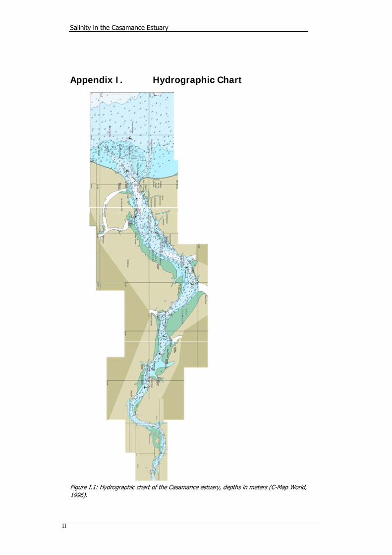
Salinity in the Casamance Estuary
II
Appendix I. Hydrographic Chart
Figure I.1: Hydrographic chart of the Casamance estuary, depths in meters (C-Map World, 1996).

Occurrence and Consequences
III
Appendix II. Measurements
During the time in Senegal, several measurements were done in the Casamance estuary. September 9th springtide measurements are done during eleven hours. This measurement is done to check the predictions of the water level of Total Tide™. September 20th three measurements are made simultaneously at Ziguinchor, Goudomp and Sedhiou. This measurement is done to get information about the propagation of the tide through the estuary. The third measurement is done September 27th at Île de Karabane to check the tidal range predicted by Total Tide™ in Pointe de Diogué, which is near Île de Karabane.
Figure II.1: An overview of the measurement locations in the Casamance. The six lines are the measured cross-sections.

Salinity in the Casamance Estuary
IV
Waterlevel and velocity on 09-09-2006
4,00
4,204,40
4,60
4,805,00
5,20
5,40
5,605,80
6,00
0:00 2:00 4:00 6:00 8:00 10:00 12:00 14:00 16:00 18:00 20:00 22:00 0:00
time (hh:mm)
leve
l rel
ativ
e to
MW
L (m
-2,00
-1,60-1,20
-0,80
-0,400,00
0,40
0,80
1,201,60
2,00
velo
city
(m
/s)
waterlevel Total Tide velocity
September 9th 2006, springtide Location: bridge at Ziguinchor (N12˚35,359' W16˚15,758') Figure II.2: measurements of velocity and relative water level. Important characteristics: phase lag ε = 1.442 rad = 0.459π tidal excursion E = 15077m September 20th 2006, springtide Locations: bridge Ziguinchor (N12˚35'359, W16˚15'758)
port Goudomp, (N14˚47'287, W15˚53'172) Hotel Palmeraie Sedhiou (N.12˚39'293, W15˚31'174)
Distance to estuary mouth (km)
Delay relative to Ziguinchor (hr)
Phase lag (-)
Tidal range (m)
Ziguinchor 63 0,00 2,00 0,640 Goudomp 112 4,50 1,50 0,245 Sedhiou 170 9,00 1,00 0,210
Table II.1: Measured tidal parameters at three locations along the Casamance estuary at September 20th, 2006. tidal damping δ = 0,91m-1

Occurrence and Consequences
V
Tidal wave through Casamance river at 20-09-2006(relative to ML)
-40,00-30,00-20,00-10,00
0,0010,0020,0030,0040,00
6:00 7:00 8:00 9:00 10:00 11:00 12:00 13:00 14:00 15:00 16:00 17:00 18:00 19:00 20:00
Time (hh:mm)
Rel
ativ
e w
ater
leve
l (cm
)
Water level Goudomp Water level Ziguinchor Water level Sedhiou
Figure II.3: Propagation of the tide through the Casamance estuary. September 27th 2006, springtide Location: Île de Karabane (N12˚34'423 ,W16˚43'824) Tidal range: 1.60m Cross sections This is an overview of the measured cross sections in the Casamance, ordered from upstream to downstream. Their location can be seen in the beginning of this appendix in figure (II.4)
Sedhiou I
-2.5
-2
-1.5
-1
-0.5
00 250 500 750 1000 1250 1500 1750 2000
Distance to southern bank (m)
dept
h (m
)

Salinity in the Casamance Estuary
VI
Sedhiou II
-5
-4
-3
-2
-1
00 250 500 750 1000 1250 1500 1750 2000
Distance to southern bank (m)
dept
h (m
)
Goudomp II
-3.5-3
-2.5-2
-1.5-1
-0.50
0 500 1000 1500 2000 2500 3000
Distance to southern bank (m)
dept
h (m
)
Goudomp I
-7-6-5-4-3-2-10
0 250 500 750 1000 1250 1500 1750 2000
Distance to southern bank (m)
dept
h (m
)

Occurrence and Consequences
VII
ZiguinchorI
-15
-12.5
-10
-7.5
-5
-2.5
00 100 200 300 400 500 600 700 800
Distance to south bank (m)
Wat
er le
vel (
m)
ZiguinchorII
-25.00
-20.00
-15.00
-10.00
-5.00
0.000 250 500 750 1000 1250
Distance to south bank (m)
Wat
er le
vel (
m)
Figure II.4: Cross sections measured in the Casamance in Septemer 2006.

Salinity in the Casamance Estuary
VIII
Appendix III. Hydrological Data
aerial rainfall mm/month
year January February March April May June July August September October November December
1970 47 100 235 455 199 48 1
1971 6 104 255 289 276 74 4
1972 4 57 206 270 176 73 2
1973 7 138 231 440 183 32 0
1974 5 24 319 344 301 50 4
1975 2 15 448 395 512 62 0
1976 25 100 257 373 229 126 18
1977 0 71 194 202 280 72 0
1978 5 103 380 416 199 112 9
1979 25 170 234 248 170 69 12
1980 0 43 153 253 258 23 0
1981 31 116 341 344 189 115 0
1982 18 87 214 329 148 95 0
1983 22 105 197 185 201 30 2
1984 14 271 262 233 177 39 4
1985 0 79 217 302 320 25 0
1986 0 61 168 341 302 82 0
1987 7 158 202 355 287 79 0
1988 18 79 244 436 279 57 0
1989 1 143 278 322 293 156 0
1990 0 64 245 446 219 82 0
1991 0 36 288 266 166 101 0
1992 17 67 284 313 224 39 0
1993 3 106 343 367 300 54 0
1994 10 127 335 300 330 99 8
1995 8 86 243 350 265 59 0
1996 8 60 349 309 304 28 3
1997 42 144 158 386 348 30 0
1998 0 63 280 348 362 56 0
1999 6 154 270 533 270 193 2
2000 0 101 294 285 271 136 0
2001 0 156 278 260 262 47 2
2002 6 65 125 199 289 88 0
2003 15 138 301 438 272 139 0
2004 26 115 310 274 189 67 0
min 0 15 125 185 148 23 0
max 47 271 448 533 512 193 18
average 11 100 261 332 259 75 2
Table III.1: Aerial average monthly rainfall for the Casamance catchment 1970-2004 (edited data from DRDR).
Yearly Precipitation
y = -5,8112x + 1660
0
500
1000
1500
2000
2500
1918
1922
1925
1928
1932
1935
1938
1941
1944
1947
1950
1953
1956
1959
1962
1965
1968
1971
1974
1977
1980
1983
1986
1989
1992
1995
1998
2001
2004
Year
Prec
ipita
tion
(mm
)

Occurrence and Consequences
IX
Precipitation July
y = -0,8438x + 368,29
0
100
200
300
400
500
600
700
1918
1922
1925
1928
1932
1935
1938
1941
1944
1947
1950
1953
1956
1959
1962
1965
1968
1971
1974
1977
1980
1983
1986
1989
1992
1995
1998
2001
Year
Prec
ipita
tion
(mm
)
Precipitation August
y = -2,9317x + 605,83
0100200300400500600700800900
1000
1918
1922
1925
1928
1932
1935
1938
1941
1944
1947
1950
1953
1956
1959
1962
1965
1968
1971
1974
1977
1980
1983
1986
1989
1992
1995
1998
2001
Year
Prec
ipita
tion
(mm
)
Precipitation September
y = -0,4137x + 357,06
0
100
200
300
400
500
600
700
1918
1922
1925
1928
1932
1935
1938
1941
1944
1947
1950
1953
1956
1959
1962
1965
1968
1971
1974
1977
1980
1983
1986
1989
1992
1995
1998
2001
Year
Prec
ipita
tion
(mm
)
Figure III.1: Yearly precipitation and monthly (the 3 most rainy months) over the period 1918 – 2004, with trend analysis (edited data from DRDR).

Salinity in the Casamance Estuary
X
open water evaporation January February March April May June July August September October November December
(mm/mth) 162.8 176.8 227.1 237.4 220.7 165.1 141.2 127.7 142.3 161.4 155.9 137.5
(m/mth) 0.1628 0.1768 0.2271 0.2374 0.2207 0.1651 0.1412 0.1277 0.1423 0.1614 0.1559 0.1375
Qf Kolda m3/s
January February March April May June July August September October November December
1970 1.78 1.23 0.78 0.49 0.35 1.12 2.07 12.03 10.29 3.43 1.97 1.57
1971 1.75 1.61 1.56 1.48 1.43 1.58 11.45 14.41 12.71 6.33 2.27 1.77
1972 1.60 1.32 1.11 0.97 0.86 0.45 0.50 4.48 2.98 1.59 0.81 0.42
1973 0.26 0.20 0.16 0.10 0.08 0.34 3.72 14.43 8.22 3.24 1.22 0.49
1974 0.23 0.10 0.03 0.00 0.00 0.17 8.13 4.74 6.99 3.13 1.05 0.50
1975 0.42 0.18 0.06 0.00 0.00 0.02 2.05 5.62 35.26 11.08 2.77 1.48
1976 1.00 0.65 0.36 0.17 0.07 0.07 2.93 7.26 7.56 6.33 1.52 0.91
1977 0.82 0.57 0.43 0.13 0.05 0.06 1.27 0.92 2.53 1.25 0.42 0.14
1978 0.11 0.07 0.09 0.09 0.05 0.14 0.67 3.11 6.70 3.04 1.05 0.52
1979 0.34 0.14 0.00 0.00 0.13 0.85 3.10 3.55 3.62 1.18 0.97 0.52
1980 0.45 0.20 0.05 0.00 0.00 0.00 3.72 3.71 5.76 2.75 0.70 0.11
1981 0.23 0.04 0.00 0.00 0.00 0.00 0.99 4.36 2.72 1.16 0.81 0.54
1982 0.30 0.24 0.25 0.11 0.04 0.29 0.78 1.35 1.55 0.56 0.09 0.04
1983 0.06 0.09 0.02 0.00 0.00 0.00 1.71 0.52 0.97 0.56 0.05 0.00
1984 0.00 0.00 0.00 0.00 0.00 0.29 0.04 0.25 1.60 0.83 0.08 0.02
1985 0.01 0.00 0.00 0.00 0.00 0.00 0.10 0.61 3.02 0.53 0.03 0.02
1986 0.00 0.00 0.00 0.00 0.00 0.00 0.67 1.15 5.13 3.48 0.51 0.17
1987 0.05 0.12 0.01 0.00 0.00 0.00 1.09 0.93 2.77 1.40 0.07 0.00
1988 0.00 0.00 0.01 0.00 0.00 0.00 0.00 8.18 4.23 1.36 0.46 0.16
1989 0.11 0.06 0.01 0.00 0.00 0.78 0.73 1.84 2.83 2.27 0.85 0.23
1990 0.03 0.01 0.00 0.00 0.00 0.39 1.88 0.90 1.21 0.60 0.17 0.03
1991 0.00 0.00 0.00 0.00 0.00 0.00 0.72 1.20 1.48 0.44 0.04 0.02
1992 0.04 0.00 0.00 0.00 0.00 0.76 0.12 1.23 3.04 1.19 1.06 0.13
1993 0.02 0.02 0.01 0.00 0.00 0.55 1.62 2.33 2.41
1994 0.81 0.47 0.27 0.21 0.19 1.02 4.22 8.19 10.77 5.76 2.23 1.24
1995 0.83 0.48 0.28 0.21 0.14 0.77 3.19 6.19 8.15 4.35 1.69 0.94
1996 0.63 0.36 0.21 0.16 0.16 0.87 3.62 7.02 9.24 4.94 1.91 1.06
1997 0.71 0.41 0.24 0.18 0.16 0.89 3.70 7.17 9.44 5.05 1.95 1.09
1998 0.73 0.42 0.24 0.19 0.17 0.91 3.79 7.35 9.68 5.17 2.00 1.11
1999 2.64 0.52 0.03 0.01 0.17 0.34 0.79 1.16 4.86 7.72 5.87 3.93
2000 0.98 0.09 0.05 0.05 0.04 0.72 6.24 13.14 11.36 7.58 2.89 1.22
2001 0.78 0.58 0.16 0.11 0.00 0.00 3.90 6.69 5.80 2.46 0.90 0.18
2002 0.12 0.11 0.09 0.06 0.04 0.01 3.79 5.10 10.08 8.87 2.56 0.99
2003 0.26 0.15 0.10 0.05 0.00 2.89 2.71 6.14
Min 0.00 0.00 0.00 0.00 0.00 0.00 0.00 0.25 0.97 0.44 0.03 0.00 Max 2.64 1.61 1.56 1.48 1.43 2.89 11.45 14.43 35.26 11.08 5.87 3.93 Mean 0.53 0.31 0.19 0.14 0.12 0.48 2.53 4.92 6.51 3.43 1.28 0.67
Table III.2: Average monthly open water evaporation (based on ClimWat database) and fresh water discharge distribution at Kolda station from 1970 until 2003 (edited data from DRDR).

Occurrence and Consequences
XI
Appendix IV. Measured salinity; Calibration dataset
Salinity in g/l from Thiam et al., 1998Station no 12 15 17 18 19 22 23 24 28 30 32 33 34 38 42X (km) 63 89 103 106 109 122 128 136 161 179 192 198 200 223 254afstand 26 14 3 3 13 6 8 25 18 13 6 2 23 31
15-6-1987 48,7 55,4 57,7 58,3 61,2 67,4 72,5 85,1 91,5 101 103 45,615-7-1987 46,4 53,3 56,3 56,6 59,4 61,1 64,5 68,2 80,5 85,4 85,2 91,1 47 8,215-8-1987 41,3 44 46,4 44,4 50,9 53,9 55,6 50,6 61,4 57,5 46,4 45,1 4,2 0,115-9-1987 29,4 29,8 32,9 31,7 28,3 32,1 35,5 33,2 34,6 32,9 18,6 8,6 7 1,2 015-10-1987 27,5 26,9 29,4 28,8 27,9 30,8 32,1 32,5 29,6 25,5 13,4 8,9 6,6 1,4 0,215-11-1987 28,2 30,2 30,6 31,2 31 31,3 32,4 31,3 30 27 18,1 13,1 10,4 3,5 0,915-12-1987 31,3 33,4 33,4 34,6 33,4 34,5 34,6 33,6 34,6 31,1 22,1 17,4 14 5,7 1,515-1-1988 32 36,4 36,8 37,5 36,6 37,3 37,1 37 38 34 26,1 22,8 17,5 7,4 1,915-2-1988 33,6 35,8 36,4 38,5 37,5 38,4 39,2 39 40,1 39,8 35,3 34,9 29,8 16,4 2,215-3-1988 35,5 37,1 38,1 39,2 39,2 40,1 42,5 40,5 42,3 44,7 44,5 45,2 42,8 32,1 2,915-4-1988 36,8 37,9 39,8 41,4 41,2 41,9 43,2 43,4 45 48,6 62,7 55,6 54,4 53 4,715-5-1988 37,4 38,7 40,8 43,5 40,5 42,9 43,5 44,2 49,3 51,9 59,8 62,9 62,9 72,7 15,915-6-1988 39,1 40,7 41,2 42,8 40,3 43,2 44,1 45 48,8 55,3 62,3 69,4 69,4 80 4215-7-1988 47,2 55 57,1 58,1 67,9 58,5 60,6 62,6 67,1 75 86,1 91,3 94,8 88,6 40,915-8-1988 38,5 39,5 45 43,3 47,6 47,6 49,8 60,8 47,6 65,8 61,6 62 52,1 12 0,615-9-1988 26,7 22,9 32,9 36,9 35,8 39,3 39 38 21,2 30,1 13,5 5,6 7,7 0,8 015-10-1988 22,9 25,2 26,6 29,4 27,4 30,5 31,9 29,8 26,1 21,7 9,5 6,5 2,2 0,315-11-1988 28,5 28,1 30,3 29,3 29,7 32,4 32,4 29,1 29,3 26,1 15,6 10,5 4 0,615-12-1988 31,2 33,3 35,2 35 35 35,2 36,2 33 33,5 29,3 19,7 15,5 13,2 5,5 1,315-1-1989 32,5 36,7 38,5 38,5 36,8 37,7 40,2 37,8 38,5 34,3 26,4 21,2 12,3 1,315-2-1989 39,3 39,6 40,7 39,4 40,9 42 39 40,7 40,9 35,7 31,1 22,7 1,515-3-1989 35,5 40,3 42 43,6 40,9 40,8 41,3 40,3 41,9 43,7 42,8 42,5 40,5 34,3 1,715-4-1989 45,8 49 50,9 46,4 49,4 50,3 50,6 47,6 50 52,6 60,1 61,9 57,1 60,2 6,215-5-1989 56,4 61,6 59,9 57,9 61,1 61 62,5 58,9 59 67,4 79,5 83 82,3 98,3 47,415-6-1989 58,1 61,1 59 59,6 62,9 61,8 63,2 59,7 62,4 72,8 81,9 85,9 88,4 66,6 26,615-7-1989 46,6 54 54 55,7 47,6 52,4 55 55,1 58,1 65,2 71,4 69 69 12,6 0,415-8-1989 44,2 44 49,4 46,4 48,5 52,3 51,1 50,9 47,8 57,3 52,2 44,2 38 2,3 0,215-9-1989 34 34,8 38,2 39,8 39,8 40,5 40,3 34,6 35,1 42,4 21,2 19,8 8,8 1,9 0,215-10-1989 32,8 33,1 35 34,4 35,3 37,1 38,2 32 31,8 29,2 13,6 6,2 3,9 2,1 0,215-11-1989 35,5 36,3 36,1 33,1 37,1 38,6 39 36,6 35,2 27 14,4 7,6 5,6 4 0,415-12-1989 38,5 40,2 39,7 41,1 40,3 41,9 41,5 38,7 38 29,7 19,7 9,9 8,1 5,2 0,815-1-1990 39,6 43,9 43,7 44,1 45,2 44,3 43,3 39,8 41,6 33,2 20 13,8 14,6 7,1 1,115-2-1990 42 44,5 45 48 46,3 46,9 46,9 42 45,9 43,8 33,7 28,4 25,6 15 1,515-3-1990 45,6 48,4 49,5 50,9 49,9 49,6 51,3 47 48,5 50,3 46 37 38,5 27,8 1,815-4-1990 51,2 54,8 56,6 58,7 56,9 55,1 53,6 53,9 54,7 60,8 60,5 68,6 57 51,2 4,815-5-1990 53,9 57,9 60,1 61,5 60,7 60,9 59,2 59,5 60 68,5 75 77,3 76,6 87,6 17,915-6-1990 57,1 78,4 63,8 65,8 63,3 66,5 67,4 67 68,4 78 83,5 92,9 93,6 116 45,415-7-1990 52,6 50,5 58,4 63,6 53,5 65 67,1 64,5 65,5 78 83,9 95,8 85 55,5 56,915-8-1990 42 39,4 44,3 52,2 38,4 59,4 61,5 53 57,5 69,3 68,8 50,1 44,9 42,9 31,615-9-1990 30,2 37,6 44,5 48,4 44 55,1 56,6 54,2 51,7 55,1 34,1 27,9 19,4 3,3 3,715-10-1990 30,4 38,4 43,8 47,8 40,7 52,1 54,7 62,7 48,5 53,2 38,5 22,4 21,1 4 0,215-11-1990 36,8 43,6 45,5 49 51,5 53,5 66,1 55 53,6 57,6 29,2 6,4 0,915-12-1990 42,7 48 49,7 52,3 53,2 57,4 68,5 68,9 58,9 83,7 8,1 1,315-1-1991 45,3 52,4 51,8 54,9 58,2 59,3 64 61,9 63,8 69,7 69,2 69,3 65,8 17,1 1,515-2-1991 47,8 53,4 57 61 59,7 61,6 67,3 66,3 68,6 74,6 79,1 75 39,4 1,715-3-1991 50 55,7 57,8 60,8 60,1 63,4 68,6 70,2 74,5 80,4 95,1 93,4 79,8 2,615-4-1991 53,6 60 61,8 65,1 64,3 67,5 70,1 74 80,8 92,7 106 88,5 117 132 66,815-5-1991 58,6 63,1 65,8 66,3 66,2 71 73,7 76,4 84,2 96,3 116 134 129 171 11715-6-1991 60,4 65,2 68,2 68,4 73,2 73,3 74,8 79,5 81,7 90,6 125 135 137 164 12915-7-1991 59,6 62 59,8 71 67,5 73,7 76,6 81,2 57,4 105 110 133 134 146 12215-8-1991 49 44,5 50,3 60,6 68 64,3 66,6 69,4 57,4 97,1 97,8 96,6 86,9 17 3,715-9-1991 36,6 49,2 48,3 47,3 53,1 56,1 57,4 87,9 82,7 72,8 73 49 5,8 1,515-10-1991 35,6 31,6 42,4 45,9 42,1 46,4 48,9 47,5 62,3 68,6 59,1 45,8 5,8 2,215-11-1991 30,8 35,4 37,9 39 42 42,9 43,5 44,5 53,2 63,1 59,4 43,4 10,7 715-12-1991 33,6 37,7 39,3 40,9 42,7 44,5 47 45 56,5 69,2 64,3 53,4 22,2 15,815-1-1992 35,6 39,1 40,7 41,9 43 47,8 52,8 48,7 59,2 71,8 70,4 62,5 42,3 20,315-2-1992 38,6 43,5 42,2 46 46,3 52,2 56 54,4 63,7 71,7 81,8 82,6 68,7 61,4 21,115-3-1992 51,5 55,7 56 62,6 62,4 66,8 70,9 72,5 81,2 100 113 128 60,7 121 29,215-4-1992 54 58,3 60,4 64 62,9 68,5 71,7 76,1 85,8 103 118 139 72,3 171 74,915-5-1992 55,9 59,5 60,5 63,2 66,5 70 73,2 75,9 87,4 100 125 152 95,4 188 12715-6-1992 49,1 51,8 59 57,6 58,6 72,4 73,8 80 90,7 113 139 124 126 14315-7-1992 49 53,1 69,4 55 56,9 72,7 80 90,4 107 118 120 129 80,5 Table IV.1: Salinity levels at different stations in the main course of the Casamance estuary from June 1987 until July 1992 (Thiam et al., 1998).

Salinity in the Casamance Estuary
XII
Figure IV.1: Locations of the measurement stations along the Casamance estuary (Pagès et al., 1987).

Occurrence and Consequences
XIII
Appendix V. Conclusions
L’estuaire de la Casamance devenait hyper salin à la fin des années 70 par une diminution de pluie. Les hautes concentrations de sel ont beaucoup influencé la flore et la faune. Certaines plantes meurent et laissent de grandes plaines arides. La diminution de pluie a duré jusqu’au milieu des années 90, et après, un petit rétablissement s’est installé. Pourtant, la quantité de pluie n’est pas encore au même niveau des années 60.
On a recherché l’hyper salinité de la Casamance à l’aide d’un modèle de l’intrusion de sel. On a constaté que pour des années successives ayant la même quantité de pluie, la répartition de sel suit un patron à travers l’année. À la fin de la saison pluvieuse (de juin à octobre), les concentrations de sel sont plus bas qu’à la fin de la saison sèche. On trouve les plus hautes concentrations plus en aval de la rivière à la fin de la saison pluvieuse qu’à la fin de la saison sèche. La raison de ses effets est la variation dans l’écoulement de l’eau douce, renouvelant l’eau salée, pendant la saison pluvieuse. Les résultats après avoir surveillé quelques scénarios (cités ci-dessus) sont :
• On a besoin d’une quantité de pluie deux fois la moyenne pendant une année pour changer l’estuaire de la Casamance en un estuaire normal.
• Plusieurs années plus pluvieuses qu’en moyenne ne sont pas suffisantes pour avoir de nouveau un estuaire normal; seulement un nouveau équilibre est atteint.
• La distribution de sel s’adapte plus vite à une augmentation de l’eau douce qu’à une diminution.
• Quand la pluie est plus repartie dans l’année, l‘estuaire devient plus hyper salin.
• Il y a une limite à la plus haute distribution de sel dans l’estuaire, qui a une forme exponentielle dans la partie qui subit la marée.
La relation entre l’estuaire et la gestion de l’eau dans la région de la Casamance a été recherchée pour mieux comprendre l’importance des processus concernés et pour situer la recherche dans un cadre plus étendu. Cela aide à trouver des relations entre plusieurs problèmes et leurs conséquences et à trouver des endroits exposés à des risques.
• L’hyper salinité est le problème le plus important dans la partie en amont de l’estuaire, où l’influence de la marée est petite. Ceci a des conséquences négatives pour l’agriculture et la pèche, ce qui empêche la développement de la région. Puisque la salinité n’y augmentera probablement pas, il faut attirer l’attention sur la prévention de la pollution de l’eau potable par l’intrusion du sel et sur les techniques pour extraire du sel marin.
• Des acides potentiels sont des conditions préalables pour l’agriculture dans la plaine en aval. Une bonne gestion y est nécessaire pour prévenir des problèmes.
• L’érosion et la sédimentation sont des problèmes dans les endroits urbains. Des constructions qui sont mal protégées dans un terrain incliné sont très susceptible d’érosion extensive. Sédiment érodé peut tomber dans et saliner des rizières situées plus basses. Il faut une approche intégrale pour améliorer

Salinity in the Casamance Estuary
XIV
la situation. La prévention d’érosion est la meilleure solution pour commencer. Des canaux de drainage dans la ville préviennent le dégât de routes et végétation et une clôture peut diminuer l’érosion.
• On a construit des digues anti-sel pour prévenir l’intrusion du sel et pouvoir dégager des pièces de terre de sel pour l’agriculture. Les succès sont inégaux, parce que l’acidification de la terre se produit dans certains cas. La terre en amont de la digue peut être rincée du sel. L’effet sur les environs est grand. Beaucoup de mangroves mourront, le transport du sédiment et nutriments change et les terres à frayer pour différentes espèces d’animaux ne sont plus accessibles. L’effet sur l’estuaire est difficile à calculer.

Occurrence and Consequences
XV
Appendix VI. Images en Français
Image V.1: Le management d’eau dans le basin de l’estuaire Casamance.

Salinity in the Casamance Estuary
XVI
Image V.2: Barrage anti sel construé loin de l’embouchure.

Occurrence and Consequences
XVII
Image V.3: Barrage anti sel construé au fin de l’embouchure.


![Supplementary Materialweb.media.mit.edu/~gordonw/TensorDisplays/TensorDisplays-Supplement.pdfnotation [Cichocki et al. 2009; Kolda and Bader 2009]. Our goal is to show, in an intuitive](https://static.documents.pub/doc/80x56/5fe35532de93f927c548d29a/supplementary-gordonwtensordisplaystensordisplays-supplementpdf-notation-cichocki.jpg)


